the Creative Commons Attribution 4.0 License.
the Creative Commons Attribution 4.0 License.
 | 31 Mar 2023
Accounting for meteorological biases in simulated plumes using smarter metrics
Pierre J. Vanderbecken
Joffrey Dumont Le Brazidec
Alban Farchi
Marc Bocquet
Yelva Roustan
Élise Potier
Grégoire Broquet
In the next few years, numerous satellites with high-resolution instruments dedicated to the imaging of atmospheric gaseous compounds will be launched, to finely monitor emissions of greenhouse gases and pollutants. Processing the resulting images of plumes from cities and industrial plants to infer the emissions of these sources can be challenging. In particular traditional atmospheric inversion techniques, relying on objective comparisons to simulations with atmospheric chemistry transport models, may poorly fit the observed plume due to modelling errors rather than due to uncertainties in the emissions.
The present article discusses how these images can be adequately compared to simulated concentrations to limit the weight of modelling errors due to the meteorology used to analyse the images. For such comparisons, the usual pixel-wise ℒ2 norm may not be suitable, since it does not linearly penalise a displacement between two identical plumes. By definition, such a metric considers a displacement as an accumulation of significant local amplitude discrepancies. This is the so-called double penalty issue. To avoid this issue, we propose three solutions: (i) compensate for position error, due to a displacement, before the local comparison; (ii) use non-local metrics of density distribution comparison; and (iii) use a combination of the first two solutions.
All the metrics are evaluated using first a catalogue of analytical plumes and then more realistic plumes simulated with a mesoscale Eulerian atmospheric transport model, with an emphasis on the sensitivity of the metrics to position error and the concentration values within the plumes. As expected, the metrics with the upstream correction are found to be less sensitive to position error in both analytical and realistic conditions. Furthermore, in realistic cases, we evaluate the weight of changes in the norm and the direction of the four-dimensional wind fields in our metric values. This comparison highlights the link between differences in the synoptic-scale winds direction and position error. Hence the contribution of the latter to our new metrics is reduced, thus limiting misinterpretation. Furthermore, the new metrics also avoid the double penalty issue.
- Article
(3832 KB) - Full-text XML
- BibTeX
- EndNote


Near-real-time monitoring of atmospheric gaseous compounds at the scale of power plants, cities, regions, and countries would allow decision-makers to track the effectiveness of emission reduction policies in the context of climate change mitigation (Horowitz, 2016) or other voluntary emission reduction efforts. Inventories of the emitted atmospheric gaseous compounds are diverse in scale (Janssens-Maenhout et al., 2019; Kuenen et al., 2014) and methodology. The elaboration of comprehensive inventories generally combines various approaches based on a complex mixture of measurement techniques, database elaboration, and numerical modelling. Despite the use of quality assurance and control verifications (Calvo Buendia et al., 2019a, b), the emissions fluxes can bear large uncertainties, depending on the species, on the countries or on the spatial scale (Cai et al., 2019; Hergoualc'h et al., 2021; Meinshausen et al., 2009; Pison et al., 2018; Solazzo et al., 2021). Furthermore, the delay between the emissions and the release of the corresponding inventory could be important due to a large amount of data to gather and aggregate. Even when the inventories are known to be accurate, they currently do not fulfil the need for real-time monitoring of emissions at a regional scale. By observing from space the plumes of gases downwind of large cities and industrial plants, and atmospheric signals at a scale of a few to several hundreds of kilometres, the new generation of high-resolution satellite imagery may help address this need (Veefkind et al., 2012; Broquet et al., 2018). For instance, the future Copernicus Anthropogenic Carbon Dioxide Monitoring (CO2M) mission will provide images of CO2 concentrations at a resolution of almost 2 km2, which will enable the observation of urban-scale pollutant plumes (Brunner et al., 2019; Kuhlmann et al., 2019, 2020). These new images can be directly used through fast methods to quantify the mean emissions of sources (Varon et al., 2018, 2020; Hakkarainen et al., 2021). These fast methods only require images to estimate the emissions. They do so either by using a simplified chemical transport model (CTM) or by averaging the emissions of a given source.
Here we focus on the use of such images to update the emissions sources on a smaller timescale. This can be done using an inverse method relying on comparisons between the images and the predictions of a CTM. A better match between the observed concentration fields and the simulated one will result from a more accurate source. However, the CTM prediction is bounded by the meteorological conditions used. It takes as inputs temperature, pressure, winds, cloud cover fields, etc. Usually, these atmospheric fields are provided by predictions previously obtained with mesoscale numerical weather prediction models (Lian et al., 2018). The estimated atmospheric fields come with uncertainties, which in turn yield uncertainties in the simulated concentration fields, for instance, the location or the main direction of the plume. Within the retrieval algorithm, the concentration fields derived from satellites and CTM models are usually compared pixel-wise. However, pixel-wise comparison cannot easily remove the relative weight of the meteorological uncertainties within the comparison between observation and simulation. This results in estimated increments applied to the emissions inventories that are biased by the approximated meteorology used in the simulations. This issue is also present in other simulations with observation comparisons (Dumont Le Brazidec et al., 2021; Farchi et al., 2016; Keil and Craig, 2007). Assuming that the temporal variability (e.g. annual cycle, seasonal cycle, diurnal cycle) of the emissions is well-known and that the CTM is perfect, the displacement between the observed and simulated plumes is driven by the meteorological conditions. Such a displacement yields a position error in the inversion. Thus our main goal is then to define a metric for the comparison that levels down the position error to reduce the weight of meteorology uncertainties within the inversion.
A better account of position error for observation versus simulation comparison of coherent features is a subject of active research (e.g. Ebert and McBride, 2000; Ebert, 2008; Gilleland et al., 2009; Gilleland, 2021). These authors developed several metrics and skill scores that are more sensitive to pathological situations where usual metrics provide less information, especially when there is a position error between the feature they observed and the one forecasted. To do so, they build indicators by splitting the sources of discrepancies and by doing comparisons on deformed meshes (Hoffman et al., 1995; Hoffman and Grassotti, 1996; Amodei et al., 2009; Marzban and Sandgathe, 2010; Gilleland et al., 2010). We will follow the same methodology, by splitting the different sources of discrepancies, but the position errors will include errors due to a translation and a rotation. We will consider a specific class of deformations to free the comparison from position errors. We will consider either (i) an isometric transformation or (ii) a transport map resulting from optimal transport, both differentiable with respect to the compared plumes. Optimal transport metrics were already used for radionuclide plumes (Farchi et al., 2016), but there were computation limitations. To allow a more systematic comparison between the metrics, we use the Kantorovich standpoint on optimal transport.
The objective of this paper is to develop a simple and efficient metric for urban-scale plume images which can level down the difference due to the meteorology while fitting into an inverse framework (following Feyeux et al., 2018; Tamang et al., 2022). Even though the methods could be used for other gaseous compounds, reactive atmospheric gaseous compounds have a more complex transport due to chemistry. For the sake of simplicity, we will consider CO2 since it is a passive tracer. Several metric candidates are introduced and compared. From the baseline local ℒ2 norm, a new metric with an upstream non-local correction of position errors is described in Sect. 2. In Sect. 3, going further away from the local comparison, we use the optimal transport theory to define the Wasserstein distance between two plumes and then to build a new metric freed from position errors. The different metrics are then evaluated and compared on a database of analytical two-dimensional Gaussian puff cases in Sect. 4. The metrics are then compared on a realistic database of CO2 plumes from a German power plant in Sect. 5. For both databases, the images and the simulations are computed using the same model, which allows us to monitor the discrepancies seen by the metrics. In Sect. 6 we describe the dependence of the four metrics on meteorology, before concluding in Sect. 7.
In this section, we start by introducing the notation in Sect. 2.1 and then the Gaussian puff model used to simulate the plumes in the analytical experiments in Sect. 2.2. Furthermore, we assume that the plumes are already detected and separated from the background noise and instrumental noise. These steps bring challenges that are outside the scope of this article. The ℒ2 norm is then defined in Sect. 2.3, with an emphasis on the double penalty issue. To deal with the double penalty issue associated with the family of pixel-wise metrics such as the ℒ2 norm, a second metric is proposed in Sect. 2.4.
2.1 Discrete and continuous representation of an image
In the present article, we focus on two-dimensional images of the enhancement of the total column of CO2 concentration or of the ground-level concentration. These images are given with a discretisation of N pixels. An image can hence be represented by a vector .
It is also possible to obtain a continuous representation of the image using interpolation (e.g. bilinear). In this case, the image is represented by a two-dimensional field defined on a finite domain 𝔼⊂ℝ2. Without loss of generality, we can assume that . Furthermore, the two-dimensional field X can be extended to ℝ2 by using zero padding outside the original domain 𝔼. If needed, a smooth transition from X to 0 can be included to avoid a sharp gradient at the boundaries of the original domain 𝔼.
For each metric definition, we will use either the discrete or the continuous representation of the images, but this will be explicitly mentioned.
2.2 Analytical plumes
Our Gaussian puff model is a simplified model of a concentration field (e.g. concentration at a given altitude or total column concentration in specific conditions). It has the advantage of yielding analytical expressions for the Wasserstein metrics (see Sect. 3). It is also a relevant case in transport modelling: the transport of a three-dimensional Gaussian puff is a simplified model to estimate the transport of non-reactive pollutants (Korsakissok and Mallet, 2009; Seigneur, 2019). A set of Gaussian puffs is used extensively in the following sections to illustrate and evaluate the metric candidates.
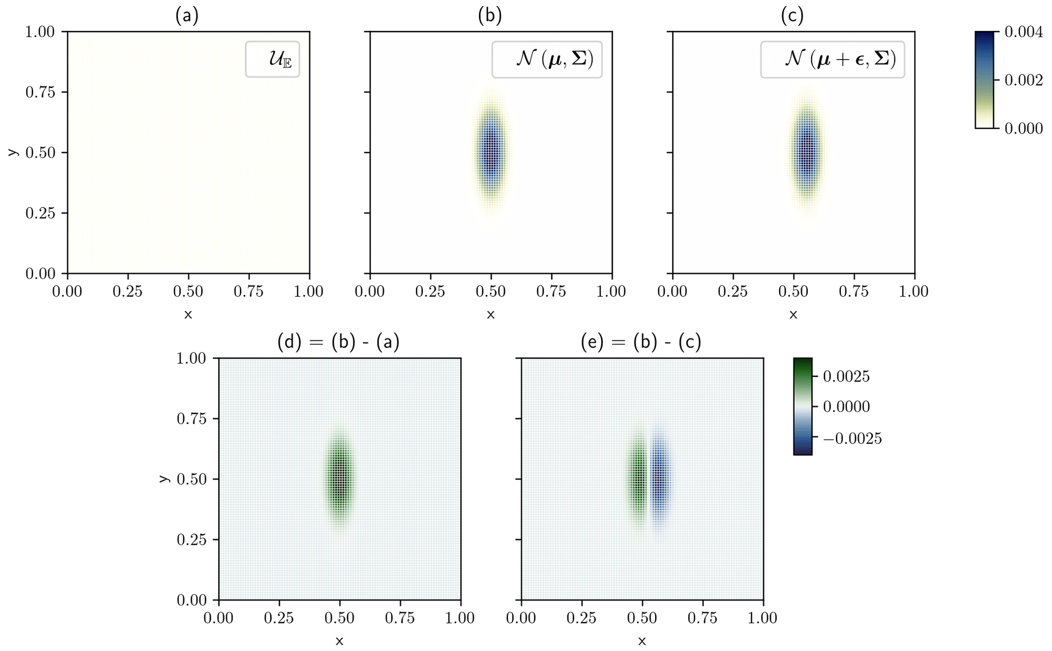
Figure 1Example of pixel-wise comparison. (a) Uniform concentration. (b) First Gaussian puff. (c) Second Gaussian puff, similar to (b) but shifted along the x axis by ϵ=0.054. (d) Discrepancies between the concentration fields (b) and (a). (e) Discrepancies between the concentration fields (b) and (c).
In the Gaussian puff model, we assume that X is proportional to the probability density function (pdf) of the normal distribution 𝒩(μ,Σ):
where μ and Σ are the mean and the covariance matrix, respectively. The operator is the determinant for square matrices. Also, note that since the covariance matrix Σ is positive definite, it can be factored as follows:
where R(θ) is the rotation matrix of angle θ, the angle between the principal axis of the Gaussian and the x axis, and where Δ is a diagonal matrix with the variance along the two principal axes of the Gaussian. Two examples of puffs based on the Gaussian puff model are provided in Fig. 1b and c.
2.3 The ℒ2 norm and the double penalty issue
To compare two concentration fields, one can see to what extent the fields overlap. This provides a pixel-wise (i.e. local) assessment of the discrepancies. The ℒ2 norm is then defined as the sum of the squared discrepancies. More specifically, the ℒ2 norm d between two concentration fields XA and XB is defined as
or
in the discrete case, where xA and xB are the two concentration vectors corresponding to the concentration fields XA and XB. In the limit of a higher and higher resolution, the discrete formulation should converge towards the continuous formulation.
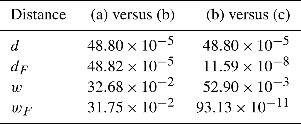
To identify the origin of the discrepancies, Feyeux et al. (2018) propose to split the difference between two fields into two categories: the position error and the amplitude error. A position error occurs when the two compared plumes are not located in the same place in the images. An amplitude error occurs when the two compared plumes are in the same place in the images, but locally their pixels do not have the same values. With the ℒ2 pixel-wise norm, all the discrepancies are seen as local amplitude errors. This property is illustrated in Fig. 1, where a uniform concentration field 𝒰𝔼 is compared to two Gaussian puffs shifted by ϵ=0.054 along the x axis with respect to each other.1 The values of the distance are reported in Table 1. In this case, a small position error is penalised by d as much as an absence of plume: this is the so-called double penalty issue. For this metric, the translation cost is composed of two equal contributions. The first is the cost of setting to zero all pixels at the location of the first Gaussian puff. The second is the cost of enhancing the pixels at the translated location.
Table 1Comparison between the distances for the example in Fig. 1. d is the ℒ2 norm, dF the ℒ2 norm with upstream position correction as defined in Sect. 2.4, w the Wasserstein distance (Sect. 3.1) and wF the Wasserstein distance with upstream position correction (Sect. 3.4). The results are not provided with units since it depends on the metric used. The metrics d and dF share the same units, while w and wF share another one.
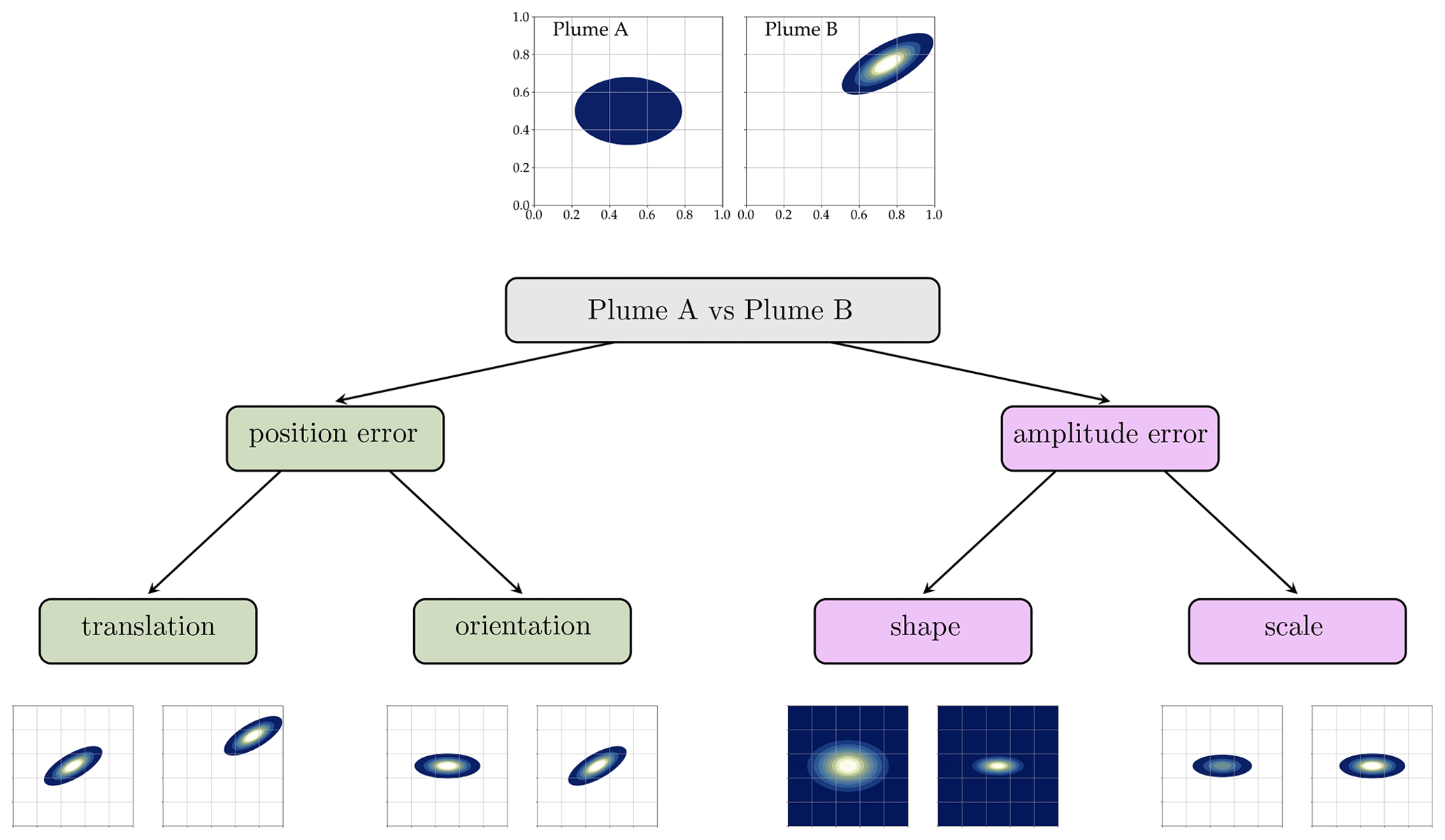
In the following sections, we further extend the classification of Feyeux et al. (2018) by splitting the amplitude error into two subcategories: the scale error and the shape error. The scale error corresponds to the difference in total amplitude between two shape-matching fields, i.e. the difference between the sum of the compared image pixels. The shape error corresponds to the difference between the isocontours after removal of the scale error (i.e. normalisation) and position error (i.e. when both centres of mass and principal axes are superimposed) fields. This splitting of errors is illustrated in the flow chart in Fig. 2.
2.4 Local metric with non-local upstream position correction
We propose to address the double penalty issue while still relying on the ℒ2 norm by applying an upstream correction of the position error to d. The position error can be seen as a combination of an orientation and a translation error. The orientation error corresponds to the differences that could be reduced by a rotation applied to two concentration fields sharing the same centre of mass location that maximises their overlapping. The translation error corresponds to the difference that could be reduced by a translation applied to two concentration fields.
The new distance is defined in a way that involves finding the rotation and translation that minimise d. The idea is that the rotation should cancel the orientation error, and the translation should cancel the translation error. Let us consider the plane transformation F defined as follows:
which corresponds to a translation of vector , followed by a rotation of angle θ and of centre x0+xt, where is the position of the centre of mass of the plume before the transformation. The transformation F depends on three parameters: . Note that this is an isometry of the plane. The optimal transformation should minimise
However, this cost function is constant for any transformation that moves all the mass of the B plume outside the domain , and by construction XB is then null. This would make the minimisation very difficult with gradient-based optimisation methods. For this reason, we add the following regularisation term to the cost function to penalise any transformation that moves the B plume outside the domain 𝔼:
This regularisation does not affect the location of the minima of dF. The final cost function is
where α is set to the average mass of the A and B plumes, and β is set by trial and error to 104. In practice, the cost function 𝒥 can be minimised with the limited-memory Broyden–Fletcher–Goldfarb–Shanno (L-BFGS) algorithm (Nocedal and Wright, 2006) that is based on the gradient of 𝒥 with respect to all three parameters θ, xt, and yt, whose expressions are given in Appendix C. To compute the gradient, the spatial partial derivatives of the concentration field XB are needed. Hence, to ensure the continuity of the partial derivatives, we use second-order bivariate spline interpolation to define the continuous concentration field XB from its original image xb. In order to avoid any issue due to the local non-convexity of the problem, we also provide a specific initialisation to the minimisation algorithm. The initial translation is then computed using the two centres of mass. Then we do orthogonal regressions to compute the principal axes of both XA and XB. The initial θ is the angle between these axes.
Finally, with the optimal transformation F∗, i.e. the one that minimises 𝒥 defined by Eq. (8), the new distance, called dF, is defined by
For the example of Fig. 1, the values of dF are reported in Table 1 and can be compared to the values of d. In the second case (distance between the two Gaussian puffs), dF is close to zero. The residual value is due to the finite resolution of the images. In the first case (distance between the Gaussian puff and the uniform concentration), dF stays similar to d because any transformation F that keeps the plume in the domain is optimal.
In this section, we introduce the Wasserstein distance, the distance of the optimal transport, as a non-local alternative to the pixel-wise ℒ2 norm.
3.1 Optimal transport and the Wasserstein distance
The optimal transport theory was first introduced in the 17th century by Monge in his famous memoir (Monge, 1781). It is based on the idea that there exists a transport plan to move masses that minimises a given cost of transport. A wider view of the problem was proposed by Kantorovich (1942) using a probabilistic approach. The field has finally regained popularity in the last few decades, in particular with the generalisation by Villani (2009).
In this section, we follow the Kantorovich approach, which means that we will use the discrete representation (see Sect. 2.1). Moreover, the theory is defined only for vectors whose coefficients are non-negative and sum up to one. While the first condition is satisfied in our case (because we work with images of pollutant concentration), the second is not. Therefore, in the following instead of working with the concentration vectors xA and xB, we will work with their normalised counterparts and :
where 1∈ℝN is the vector full of ones and x∈ℝN is either xA or xB.
The set of couplings P between and is defined by
Note that is not empty because is a coupling between and . The cost of a coupling is defined by
where is the (i,j) element of the cost matrix C penalising the transport between and . Here, it is chosen to be the square of the Euclidean distance between the ith and jth pixels of the original image. For this specific choice, the cost function 𝒥 defined by Eq. (12) has a minimum, which is obtained for a unique coupling P∗. The Wasserstein distance, the distance of the optimal transport, is then defined by
and it is actually a distance according to the mathematical definition. The proofs of these statements can be found in optimal transport textbooks (e.g. Villani, 2009).
Two interesting properties of the Wasserstein distance can be highlighted. First, this metric is defined for normalised vectors only. This means in our case that the difference in total mass between two images is entirely ignored. Alternative solutions have been proposed to take into account this difference, e.g. the one proposed by Farchi et al. (2016) or the use of unbalanced optimal transport (Chizat et al., 2018), but this is beyond the scope of the present study.
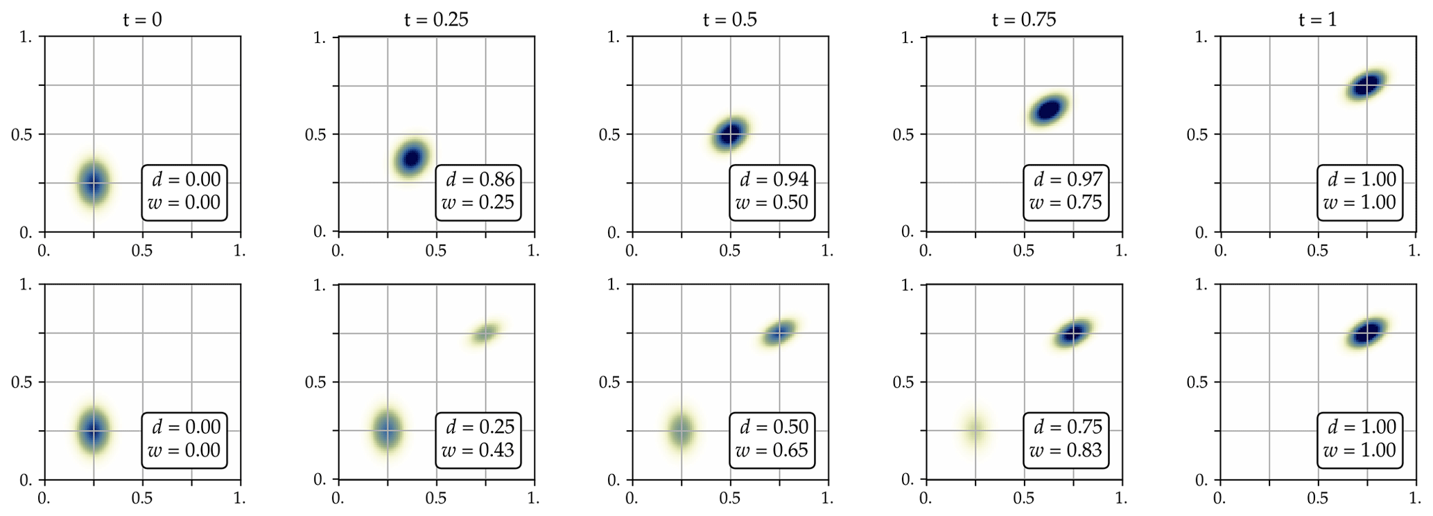
Figure 3Comparison between the optimal transport interpolation (top panels) and the liner interpolation (bottom panels). In both cases, we interpolate between two puffs using a pseudo time ranging from t=0 (interpolated puff equal to the first puff) to t=1 (interpolated puff equal to the second puff). In each panel, the legend indicates both the w and d distances between the first puff and the interpolated puff, normalised by the distance between the first and second puff. By construction, for the optimal transport interpolation w linearly grows with t, and for the linear interpolation d linearly grows with t.
Second, following Benamou and Brenier (2000), it is possible to define an optimal transport interpolation between and . This optimal transport interpolation can help us visualise the idea of vicinity according to w. An example is shown in Fig. 3 for two Gaussian puffs. In the case of the optimal transport interpolation, the w distance between the first puff and the interpolated puff is linearly growing (by the construction of the interpolation), while the increase of the d distance is at first very steep. In some sense, this behaviour was expected since the first puff and the interpolated puff are quickly separated from each other. In the case of the linear interpolation, the same phenomenon happens: the d distance is linearly growing (by the construction of the interpolation), while the increase of the w is steeper, but not as steep as the increase of d in the first case. This shows that the Wasserstein distance w is a metric that better handles the position error than d, since it accounts linearly for the mismatch in the plume positions.
3.2 Sinkhorn's algorithm
To compute the Wasserstein distance, we have to determine the optimal coupling matrix P∗ by minimising 𝒥 defined by Eq. (12). The convexity of the cost function 𝒥 is not guaranteed; thus it is usual (see, e.g. Peyré and Cuturi, 2019, and references therein) to add the following entropic regularisation:
The objective function to minimise becomes
under the same constraint . The solution of the regularised problem is an approximation of the Wasserstein distance. When ϵ→0, it converges toward the exact value of the Wasserstein distance ; when ϵ→∞, the optimal coupling matrix converges toward .
It is possible to show that minimising Eq. (15) is equivalent to minimising the Kullback–Leibler divergence between and the Gibbs kernel , where the exponential is applied entry-wise, which is given by
The advantage of this formulation it that this problem is known to admit a unique solution which is the projection of the Gibbs kernel K onto . This unique solution can be written
where u and v are vectors with positive or null entries satisfying
In these equations, ∘ is the Schur–Hadamard (i.e. entry-wise) product in ℝN.
The (u,v) factorisation is unique and can be easily found using the iterative update scheme proposed by Sinkhorn, where the lth update is given by
where ÷ is the entry-wise division in ℝN.
3.3 Log-formulation of Sinkhorn's algorithm
Sinkhorn's algorithm provides a simple and quick solution to the optimal transport problem. However, this formulation raises technical issues. The first is that for small values of ϵ – which is what we are aiming for to be as close as possible to the true optimal transport solution – the algorithm converges slowly.2 To accelerate the convergence, we use a high value of ϵ and progressively decrease it whenever (u,v) has converged. We will use this technique in our experiments.
Another numerical issue appears when ϵ is small compared to the entries of C. In this case, u, v, and K explode and cannot be computed with finite numerical precision. To address this issue, we adopt the log-Sinkhorn algorithm proposed by Peyré and Cuturi (2019), which is presented in the following lines.
Let us introduce f and g, which are related to u and v by
Instead of updating (u,v) with Sinkhorn iteration Eq. (19), we update (f,g) using
Combining the log-Sinkhorn algorithm while decreasing ϵ is not straightforward, because there are a lot of numerical decisions to make: intermediate and final values of ϵ, convergence criteria, etc. After several tests, we ended up with Appendix A, which we found to be a good trade-off between speed and accuracy. The value of ϵ is progressively decreased from 1 to 10−5: each time the convergence criterion is met, ϵ is reduced by a factor of 10. In our case, the convergence criterion is met when the relative difference between the former and the current value of the Wasserstein distance falls below . In addition, we set a maximum number of Sinkhorn iterations of 200 per value of ϵ to keep the computational cost under control. Finally, note that, for a given ϵ, one can try to accelerate the convergence by using the averaging step proposed in Chizat et al. (2018), but this is beyond the scope of the present study.
3.4 Gaussian approximation and upstream correction
Following the derivation of Sect. 2.4, we want to apply the same upstream correction of the position error to the Wasserstein distance w. However, this would require the gradient of the Wasserstein distance w with respect to each one of its inputs. The computation is not straightforward, even taking into account the log-Sinkhorn formulation developed in Sect. 3.3. For this reason, we will use the Gaussian approximation, for which the Wasserstein distance has an analytical formula.
More specifically, we assume that we have two continuous concentration fields XA and XB that follow the Gaussian puff model:
with ΣA and ΣB given by
In this case, the squared Wasserstein distance between XA and XB is given by3
Following the approach of Sect. 2.4, let us now apply the plane transformation F given by Eq. (5) to XB. The squared Wasserstein distance becomes
which depends on xt, yt, and θ, the three parameters of F. It can be shown (see Appendix D) that reaches its minimum when and (modulo π), in which case the distance is given by
which is known as the Hellinger distance between XA and XB (Peyré and Cuturi, 2019). By construction, this distance estimates the shape error between XA and XB, since the translation, the rotation, and the scale differences have been removed. In the following, it will be written wF to point out the similarity between the relationship on the one hand and on the other hand. In the case where XA and XB are not exactly Gaussian, we can still use the Gaussian puff model as an approximation. In this case, wF provides an approximation of the shape error.
Finally, an issue with both w and wF is that they are normalised fields, and thus they ignore the scale error, i.e. the difference of total mass between the images. As a consequence, these metrics cannot be used as such in an inversion framework. One way to address this issue is to add to w and wF a term to represent the scale error. Using discrete formalism, this term could be
which is convex. The remaining question would then be the relative contribution of w (or wF) and dmass in the final distance, which is related to the following question: which kind of error (position, mass, etc.) should be penalised more? This kind of question is beyond the scope of the present article, which is why we only use w and wF as is in our numerical experiments.
In this section, we evaluate and compare the metrics with a database of images built using a set of Gaussian puffs. The database is introduced in Sect. 4.1, the computation of the non-local metrics is validated in Sect. 4.2, and the behaviour of the metrics on this Gaussian puff database are compared in Sect. 4.3.
4.1 Gaussian puff database and experimental setup
The database consists of 104 pairs of images constructed using Gaussian puffs and then discretised on the domain using a finite resolution of 32×32 pixels. Each puff is parameterised by its mean μ (two scalars) and its covariance matrix (three scalars: θ and both diagonal entries of Δ), which are randomly drawn as follows:
-
Both components of μ are uniformly drawn in [0.15,0.85].
-
θ is uniformly drawn in .
-
σ1 and then σ2, the two non-zero components of Δ, are drawn from a half-normal distribution with a standard deviation of 0.33. If needed, σ1 and σ2 are then swapped to ensure σ1≥σ2.
Ideally, the domain 𝔼 should cover a large majority of the mass of each puff. In practice, more than 99 % of the mass of a Gaussian puff is covered by the 6σ1×6σ2 rectangle centred on μ and oriented along the principal axes. For this reason, we repeat step 3 of the random draw until this 6σ1×6σ2 rectangle is included in the domain 𝔼. In addition, the puffs should not be too small, which is why in our case when 6σ1 and 6σ2 are both smaller than 9 pixels, it is rejected and entirely re-drawn.
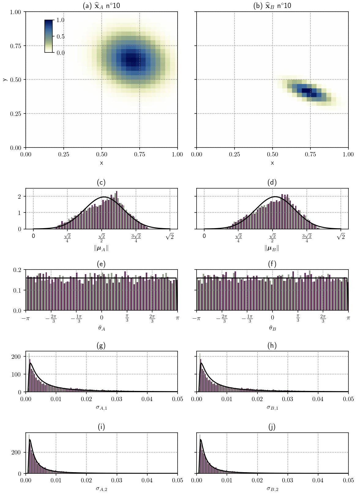
Figure 4Characteristics of the Gaussian puff database. (a, b) Images A (a) and B (b) number 10. (c–j) Histograms of (c), (d), θA (e), θB (f), σA,1 (g), σB,1 (h), σA,2 (i), and σB,2 (j).
The characteristics of the database are shown in Fig. 4 and cover the analytical pathological situations described in Davis et al. (2009). As expected, the distribution of is close to Gaussian, the distribution of θ is close to uniform, and the distribution of σ1 and then σ2 are close to log-normal.
4.2 Validation of the implemented Sinkhorn algorithm
For our Gaussian puff database, there are four different ways to compute the Wasserstein distance:
-
The analytical formula Eq. (24) can be used with the exact values of μA,B and ΣA,B. This approach will be called wth.
-
The analytical formula Eq. (24) can be used but with μA,B and ΣA,B being the sample mean and covariance of the 32×32-pixel images. This approach is closer to what will be practically done for real image plume, extracting information only from the image, and it will be called wnum.
-
The network simplex algorithm (Bonneel et al., 2011) can be used to find the exact solution of the optimal transport problem using the images like wnum. This approach will be called wemd.
-
The log-Sinkhorn iterations can be applied using Appendix A using the images like wnum. This approach will be called wϵ.
We have applied all four methods, and the differences are shown in Fig. 5. Note that wemd has been computed using the Python Optimal Transport (POT) library (Flamary et al., 2021).
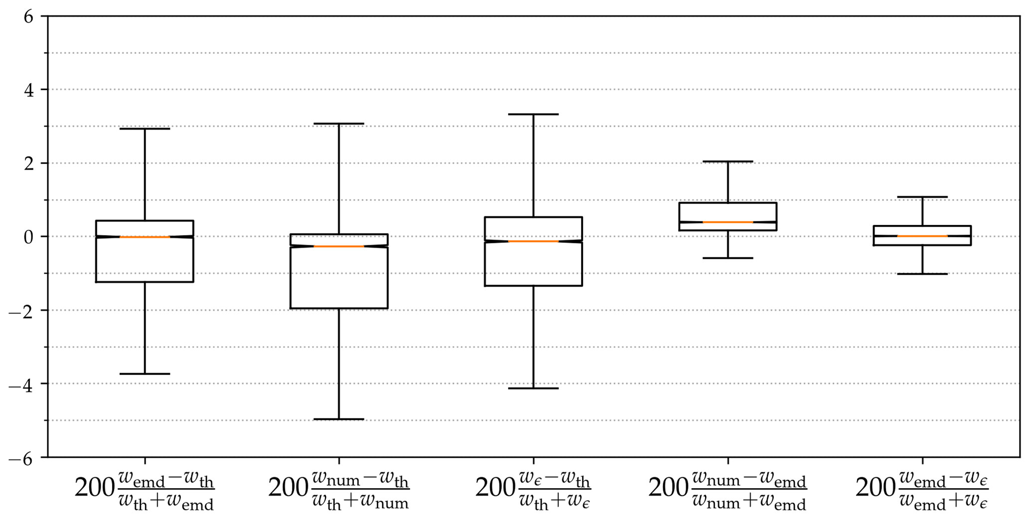
Figure 5Comparison of the different ways to compute the Wasserstein distance over the Gaussian puff database. Relative errors in percent between wemd, wth, wnum, and wϵ. The orange line is the median. Box boundaries are defined by the first and the third quartiles. The whiskers are set at 150 % of the inter-quartile range.
The fractional bias over all pairs is no more than 5 % when we compare wth to the other three methods of computing the Wasserstein distance. By contrast, wemd and wnum are very close to each other. We have checked that the latter phenomenon is reduced when the resolution is increased. Therefore, we conclude that the gap between wth on the one hand and wnum, wemd, and wϵ on the other hand is not due to the estimation of the Wasserstein distance but results from the discretisation of the problem with the 32×32 resolution (sampling errors). Figure 5 also shows that wϵ matches wemd well, which validates our log-Sinkhorn implementation.
4.3 Correlation to the different error categories
In this subsection, we compare the behaviour of the metrics with respect to three error categories: the translation error, the orientation error, and the shape error. Note that the behaviour with respect to the scale error cannot be compared since the w and wF distances use normalised images. We used the Pearson correlation as our main indicator of the strength of the link between the behaviour of the metrics and the error category. The closer the norm of the Pearson correlation is to 1, the more linear the relation between the quantities is. If the Pearson correlation is positive, then the increase in an error category leads to an increase in the metric value, if negative it leads to a decrease, and if nearly null it means that the two quantities seem independent.
For each pair of images in the database, we define T (for translation) as . This quantity represents the translation error between both images. The correlation between T and the four distances is reported in the first column of Table 2.
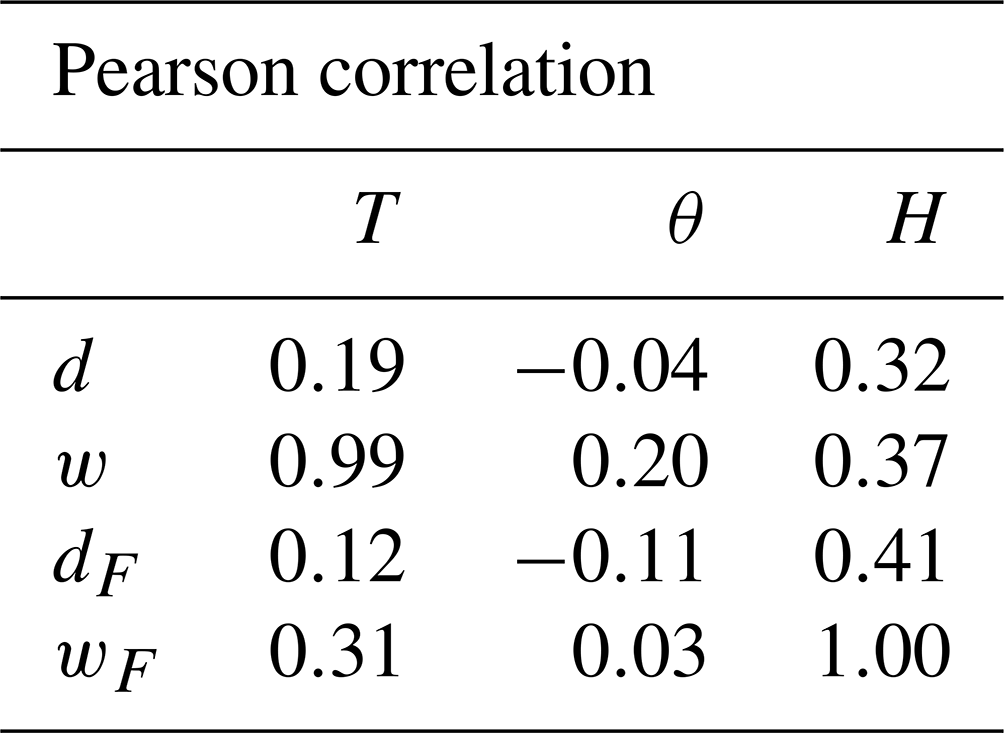
Table 2Correlations between the distances d, w, dF, and wF on the one hand and the quantities T, θ, and H on the other hand for the 104 cases in the Gaussian puff database.
As expected, the Wasserstein distance w is strongly correlated to T. The ℒ2 norm d is also showing a significant correlation of 0.33 to T, highlighting a likely dependency. Both dF and wF are designed to be released from the position error and, in particular, the translation error. This property is confirmed by the very low correlation between T on the one hand and dF and wF on the other hand. Additionally, the fact that T is much more correlated to d than to dF confirms that d indeed depends on the T quantity.
For each pair of images in the database, we define θ as . This quantity represents the orientation error between both images. The correlation between θ and the four distances is reported in the second column of Table 2. The results show also that there is no correlation between θ and any of the distances. In a sense, this shows that all the distances are, for our database, not sensitive to the orientation error.
For each pair of images in the database, we define H as the Hellinger distance between A and B, as given by Eq. (26). This is actually very similar to wF, but with one exception: H uses the theoretical values of ΔA and ΔB (i.e. the ones that have been drawn), while wF uses the sample covariance of the 32×32-pixel images. This quantity represents the shape error between both images. The correlation between H and the four distances is reported in the third column of Table 2.
Both d and w show a low correlation to H, which is not the case of dF and wF. On the one hand, the correlation between wF and H was highly expected from the definition of H. The remaining difference is due to the finite resolution of the images. On the other hand, the proportionality of dF with the H was wanted but not assessed. By superimposing optimally the plumes, we removed the position error, but dF remains sensitive to H, meaning we did not remove all errors. Thus such behaviour reflects our way of splitting the error. More generally, this comparison on the Gaussian puff database confirms that both dF and wF are freed from the position error and seem to be driven by the shape error.
To go deeper in our analysis, we now compare the metrics using realistic plumes. This section follows the same organisation as Sect. 4: we present the experimental setup in Sect. 5.1, we validate the computation of the non-local metrics in Sect. 5.2, and we compare the behaviour of the metrics on this specific database in Sect. 5.3.
5.1 Simulation database and experimental setup
We use a simulation database of hourly 3D fields of CO2 concentrations due to anthropogenic CO2 emissions from the Neurath lignite-fired power plant (Germany, 51.04∘ N, 6.60∘ E). The database is extracted from a larger one, over western Europe, as described in Potier et al. (2022). Simulations were performed with the CHIMERE Eulerian transport model (Menut et al., 2013) driven by the Community Inversion Framework (CIF; Berchet et al., 2021). The resolution of the simulation (longitude: 6.82∘ W to 19.18∘ N; latitude: 42.0 to 56.39∘ N, Fig. 6; Santaren et al., 2021) goes from 50 to 2 km. The Neurath power plant is located in the 2 km × 2 km resolution zoom (longitude: 1.25∘ W to 10.64∘ E; latitude: 47.45 to 53.15∘ N). The vertical grid is composed of 29 pressure layers extending from the surface to 300 hPa (approximately 9 km above the ground level). CHIMERE is forced by meteorological variables at 9 km resolution (Agusti-Panareda, 2018), provided by the European Centre for Medium-Range Weather Forecasts (ECMWF) for the CO2 Human Emissions project (CHE; https://www.che-project.eu/, last access: 14 March 2023). The CO2 emissions from the Neurath power plant are extracted from the ∼ 1 km (∘ × ∘) resolution inventory (TNO_GHGco_1x1km_v1_1) of the annual emissions produced by the Netherlands Organisation for Applied Scientific Research (TNO) over Europe for the year 2015 (Denier van der Gon et al., 2017; Super et al., 2020). The temporal disaggregation at the hourly scale is based on coefficients provided with the TNO inventories for the sector A-Public Power, in the Gridded Nomenclature For Reporting (GNFR) of the United Nations Framework Convention on Climate Change (UNFCCC). Emissions are projected on the CHIMERE vertical grid with coefficients corresponding to this A GNFR sector (Bieser et al., 2011), also provided with the TNO inventories. We simulate 14 d of 1 h emission pulses at the Neurath power plant location, from 1 to 14 July 2015, i.e. 336 puffs. The transport of these puffs is simulated until midnight. Consequently, the later in the day the puffs are emitted, the shorter they are tracked. Assuming that the source continuously releases CO2, the puffs are aggregated to create plume images for every hour. Due to this experimental setup, the plume follows a 24 h cycle. It appears after 0 h and grows until past 24 h of simulation and then restarts.
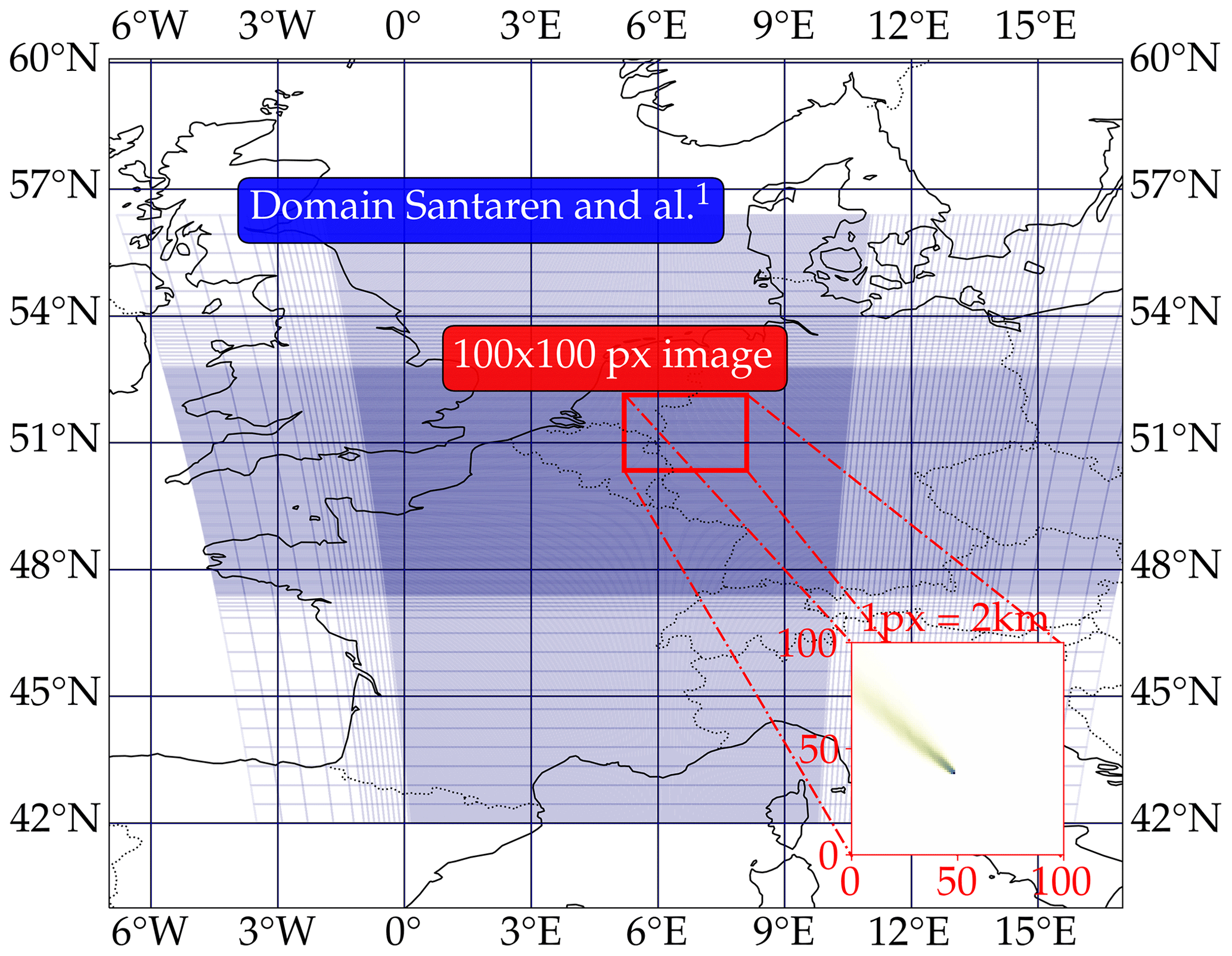
Figure 6Experimental setup. The simulation grid from Santaren et al. (2021) is in blue, centred on Belgium. The zoom in red corresponds to the vicinity around the Neurath power plant. An example of the Neurath power plant CO2 plume image is also displayed.
We ensure that the daily evolution of the hourly emission rate from the source is the same for all plumes. Hence, for a given hour of the day, the difference between two simulated plumes from two different days is due to the meteorology. We build a database that regroups per pair simulated plumes at a given hour but from different days (e.g. day 1 hour 10 versus day 3 hour 10). To get a realistic two-dimensional concentration field, we compute the vertical mean of the concentration weighted by the width of the vertical levels. We ignore the first 2 h of the simulation, to ensure that a plume appears in the image. This leaves 2093 pairs of distinct plumes. The images are cropped to 100 × 100-pixel (here 1 pixel is equal to 2 km square cell of the simulation) images to reduce the computer resource requirements.
5.2 Comparison of the different estimations of the Wasserstein distance
We have applied all three methods, and the differences are shown in Fig. 7. The results show, as for the Gaussian puff database, that wϵ and wemd are close to each other, which once again validates our algorithm. Moreover, the results show that wnum is a reasonably good approximation of w as well. The distance wnum makes the approximation that the images are Gaussian puffs, which is a strong approximation but allows for very quick computation. The values of wnum seem to be usually lower than those of wϵ. This previous remark is in agreement with Theorem 2.1 from Gelbrich (1990). It is shown that, for elliptic contour distributions with given mean and covariance matrices, the distance between the two Gaussians with these respective parameters (i.e. wnum) is a lower bound of the Wasserstein distance between the two distributions. We are not assured to work with plumes that are elliptic distributions. However, it seems to be a good direction to look at to explain and quantify, if possible, this negative bias. The understanding of the discrepancies between wnum and wϵ is needed to be able to substitute wnum to wϵ. For this reason, wnum is not tested further in the following sections.
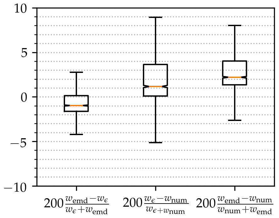
Figure 7Comparison of the different ways to compute the Wasserstein distance over the realistic database. Relative errors in percent between wemd, wnum, and wϵ. The orange line is the median. Box boundaries are defined by the first and the third quartiles. The whiskers are set at 150 % of the inter-quartile range.
5.3 Correlation to the different error categories
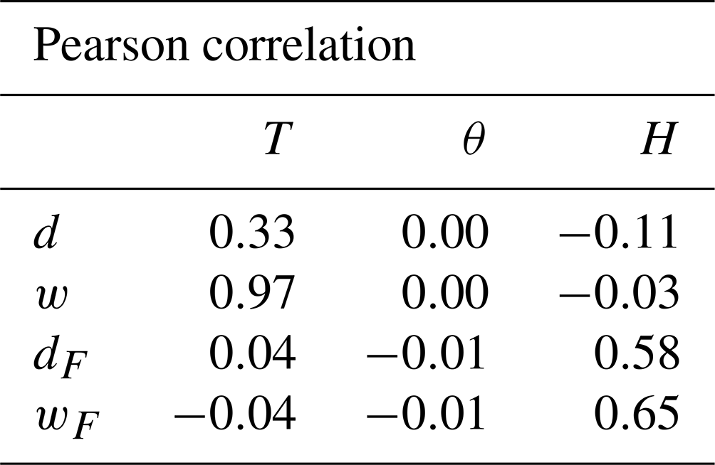
In this subsection, we compare the behaviour of the metrics with respect to the same three error categories as in Sect. 4.3: the translation, orientation, and shape error. To do so, we keep the same quantities T, θ, and H, with the notable exception that H is now equal to wF because there is no theoretical covariance. The results are reported in Table 3.
Table 3Correlations between the distances d, w, dF, and wF on the one hand and the quantities T, θ, and H on the other hand for the 2093 cases in the realistic database.
While the correlation between w and T remains very strong, d shows less correlation to T than for the Gaussian puff database. Both dF and wF are less correlated to T than d and w, respectively, but their correlation to T is here higher than with the Gaussian puff database. Hence for this realistic database, both dF and wF are only partially freed from the translation error.
In this case, the correlations between the metrics and θ are higher than for the Gaussian puff database but again do not prompt a clear conclusion.
By construction, wF is equal to H, which yields a correlation of 1. Both d and w show a small correlation to H, which was not the case in the Gaussian puff database. The correlation to H is still higher for dF, which was expected since dF is designed to be partially freed from the position error. This result, however, should be taken with caution because here, contrary to the Gaussian puff database, H now only partially accounts for the shape error between two plumes.
This second study with realistic cases shows that the behaviour of each metric slightly differs from what has been seen in the Gaussian case. Nevertheless, the results confirm that both dF and wF are partially freed from the position error while being still sensitive to the shape error, which is what we hoped for.
As stated in the introduction, the goal of this article is to develop and test metrics that can discriminate errors stemming from imperfect meteorology from other sources of discrepancies. Therefore, following the approach used in the previous sections, we define here four indicators that we consider representative of the difference in meteorological conditions between the two images. We then examine the correlation between these indicators, the previous indicators (T, θ, and H), and the metrics in the case of the realistic database.
6.1 Definition of meteorological indicators
To simplify the analysis, we define four scalar indicators that characterise the meteorological conditions. These indicators focus on the direction and the norm of the wind as experienced by the pollutant during its transportation. For each image, we proceed as follows.
-
We first average the wind components (three-dimensional fields) in the vertical direction between the surface and the planetary boundary layer (PBL) height. Indeed, the realistic database has been simulated with summer conditions, and hence the plumes are assumed to be dispersed within the PBL. This results in two-dimensional fields for each time snapshot.
-
We compute the norm and the direction of the averaged winds. This results in two two-dimensional fields for each time snapshot.
-
We average the norm and the direction over the 100×100-pixel grid. This results in two scalars for each time snapshot.
-
We finally compute the time average and time standard deviation of the averaged norm and direction between midnight (the time at which the emissions started) and the time of the image. This results in four scalars: EN (averaged wind norm), ED (averaged wind direction), SN (deviation of wind norm), and SD (deviation of wind direction).
The meteorological indicators are then defined as the absolute differences in EN, ED, SN, and SD between the two images that are compared, simply written ΔEN, ΔED, ΔSN, and ΔSD.
6.2 Correlation between the meteorological indicators and the error categories
Using the realistic database, we compute the correlation between ΔEN, ΔED, ΔSN, and ΔSD on the one hand and T, θ, and H on the other hand. The idea is to see how differences in the meteorological conditions impact the position and amplitude errors. The results are reported in Table 4.
Table 4Correlations between ΔEN, ΔED, ΔSN, and ΔSD on the one hand and T, θ, and H on the other hand for the 2093 cases in the realistic database.
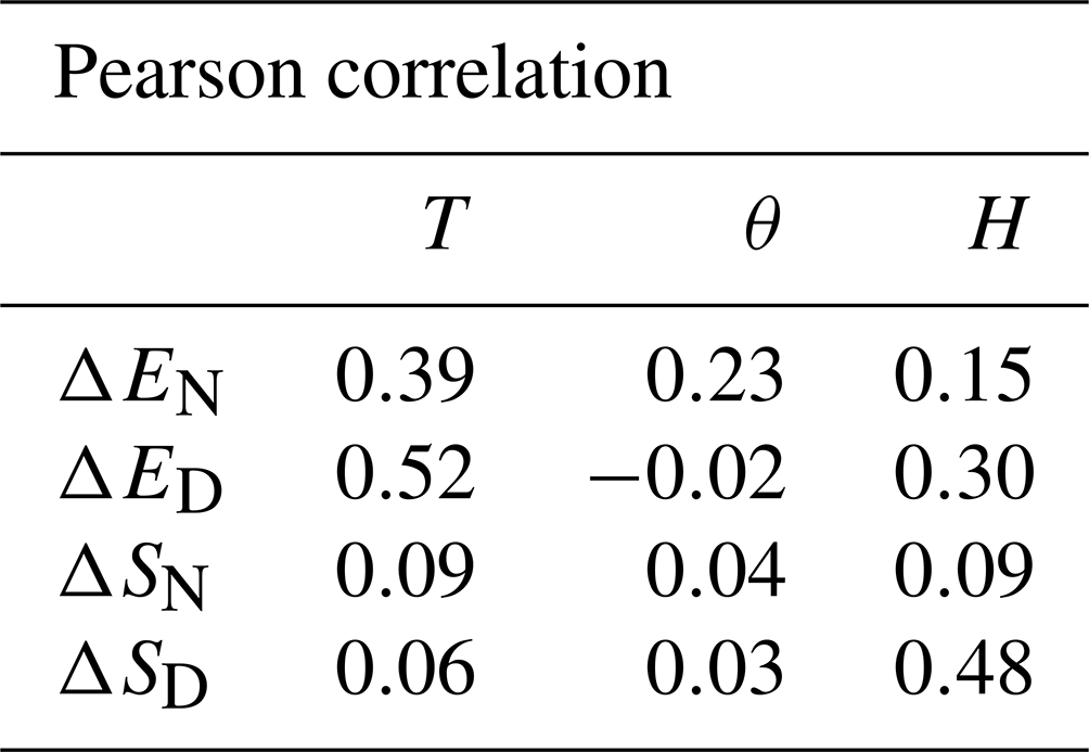
One can notice that T is mainly correlated to ΔED and a little less to ΔEN, while ΔSD and ΔED are correlated to H. This means that differences in meteorology like ΔED will likely induce both position error and shape error. Therefore, by removing the position error, we only partially remove the meteorological impact on the differences. Explaining why ΔSD induces differences in shape is straightforward, but explaining how ΔED induces differences in terms of translation instead of orientation is not as so. A difference in the main direction of the plume (which translates into ΔED) will move further away the centres of mass from each other and hence induce a larger T (which is the distance between the two centres of mass). It should be noted that a wind direction change that will keep superimposed the centre of mass will drive orientation error.
6.3 Correlation between the meteorological indicators and the metrics
To conclude our study, we now compare the different metrics to the meteorological indicators. The results are reported in Table 5.
Table 5Correlations between ΔEN, ΔED, ΔSN, and ΔSD on the one hand and the distances d, w, dF, wF, d∗, and on the other hand for the 2093 cases in the realistic database.
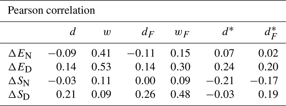
According to the correlations shown in Table 5, the metric w is correlated to ΔED and ΔEN indicators. This is expected since these meteorological changes tend to move the centre of mass and thus increase the translation error. The results show also that wF sees a drop in correlation to ΔED compared to w while getting a correlation with respect to ΔSD. For optimal transport metrics, we can see that removing the position error does not always remove the sensitivity to a change in meteorology. It should be noticed that increasing in either d or dF does not seem to be more correlated to our different meteorology indicators. Such a lack of correlation compared to the optimal transport theory metrics could result from the weight of the scale error in the distance definition. We normalised the plume the same way as we do for w before computing the distance d and dF, leading us to the normalised image distances d∗ and . First, d∗ and are more correlated than d and dF to ΔED and ΔSN, showing that the scale error is masking the sensitivity of pixel-wise metrics with respect to meteorology. Second, gains significantly in correlation to ΔSD compared to d∗ but remains as correlated to ΔED as d∗. Then the plane transformation applied in allows a better alignment of the compared plumes, giving more weight to shape error induced by ΔSD, but does not compensate for all the changes resulting from ΔED or ΔEN.
The lack of correlation to our meteorological indicators for d and dF seems appealing, but it is due to amplitude error held by a small number of highly concentrated pixels above the source for our cases (i.e. a hotspot). For similar cases, d remains a good metric for updating the inventories. If the “hotspots” of the two images have amplitudes close to each other or there is no “hotspot” but a large plume, d and dF become more correlated to several meteorological changes, making them less suitable. Pixel-wise metrics seem to be better adapted to compare “hotspot” and not highly extended plumes. A more versatile metric will be a weighted distance using the wF, or at least a normalised , which is not sensitive to all changes in meteorology, and a term that represents the scale error between the two images.
In this article, we discussed the use of new metrics for comparing passive gas plumes, practically CO2 plumes, within an inverse framework aiming at the monitoring of pollutant emissions.
At first, we emphasised how critical the double penalty issue related to pixel-wise comparison is. The traditional ℒ2 norm tends to overweight position errors mixing up with other sources of errors. In the context of source inversion, this results in an over-penalised comparison of concentration fields that are slightly shifted from each other, and the mixing makes it difficult to evaluate the relative weight of different types of error afterwards. Yet, for us, the identification of the relative weight of the errors is critical, since we want to level down the one due to meteorology and level up the one related to emissions. Assuming that most of the position error is driven by meteorology, we proposed to design metrics that are freed from position error. Following this goal, a pixel-wise metric with an upstream position correction was designed. This new metric has the advantage of keeping the formalism of the ℒ2 norm while being released from position errors. In addition, it is proposed to use a metric based on the optimal transport theory: the Wasserstein distance. Focusing on the algorithmic aspects related to two-dimensional satellite images, we derived and validated a method to compute this metric. The Wasserstein metric is more sensitive to position errors, but it is not hampered by the double penalty issue. To complete our catalogue of metrics, an optimal transport metric freed from position errors is proposed. It can be easily computed with a Gaussian approximation. This metric coincides with the Hellinger distance. Nevertheless, both optimal transport metrics rely on normalised images and thus are unaware of the difference in the total mass present in the plumes. The scale factor between the images is linearly related to emission fluxes which we want to estimate. This means that, within the inversion framework, the scale factor between the two images should be added and weighted independently.
These four metrics were compared on a specifically designed Gaussian puff database and evaluated according to their correlations with respect to translation error, orientation error, and shape error. The numerical experiments showed that the resolution of the images tends to impact the optimal transport problem. As expected, the two metrics designed to be freed from position errors are not correlated to translation and orientation errors. The ℒ2 norm and Wasserstein metrics are both correlated to the translation error. From this, we extended our tests to a realistic plume database. This second test series shows that, for a more complex plume geometry, the metrics are still correlated to the translation error. This implies that the new metrics are only partially freed from position errors.
Then we discussed the link between a position error and a variation within the mesoscale meteorology using the same realistic database. Designing relevant scalar indicators related to meteorological variance, we evaluated how specific changes in meteorological conditions lead to an increase in the distance between the plumes. We have seen that the meteorological changes can be correlated to position errors as well as amplitude errors between plumes. This means that removing the position error from the metrics will not make the comparison insensitive to a meteorological change. However, some metrics were found to be more sensitive to specific changes in meteorological conditions. For instance, while the Wasserstein metric is sensitive to changes in the main direction or intensity of the winds, the Hellinger metric is more sensitive to changes in the spread of the wind direction both in time and space. This provides guidelines to enlighten the choice of a metric for a given meteorological situation. By composing this with these new metrics freed from position error and additional scaling terms, we get more manageable metrics that will level down in the weight of modelling error due to the meteorology used in the comparison.
These metrics are used to quantify the proximity of a couple of plumes and could hence be used in an inverse framework, in particular for processing XCO2 images. The question of the impact of the meteorological changes on the metrics discussed here can be translated into another question: what importance do we give to each error category? We know that meteorological changes can result in position errors, and we strongly suspect that changes in the emission's temporal profile or vertical distribution can also yield position errors. In such a case, it would be interesting to evaluate the impact of the removal of the position errors and whether the amplitude errors carry enough information to compensate. We have seen that amplitude errors can also emerge from changes in meteorology. Thus further studies have to be undergone to evaluate the sensitivity of the metrics to either the emissions or the meteorology, to determine which error has to be more weighted from the perspective of monitoring the emissions. We have to make sure that by removing some sensitivity with respect to meteorology, we are not levelling down by the same factor the sensitivity with respect to the emissions.
For an operational purpose, optimising on non-local metrics is much more difficult than on pixel-wise metrics because it requires the computation of non-trivial gradients. The three non-local metrics that we proposed are parameterised. These parameters usually balance a trade-off between computational efficiency and accuracy. In the case of the pixel-wise distance with an upstream correction, the choice of the optimal isometry to apply depends on these parameters. Even though this study could be done with a personal computer, further computation optimisation developments are needed for operational use. Here we are only considering passive tracers, but an extension of the study should be using these metrics for reactive pollutants. However, it requires quantifying the relative impact of chemistry on the shape, scale, and position of the plume.
The key idea here is that meteorology is fixed and bounds our model predictions. We choose to develop metrics that aim to remove the weight of such bound within the comparison to the observation. We could instead consider that meteorology is not fixed and can be seen as additional degrees of freedom to estimate. Thus the Wasserstein metric is interesting because it penalises the position error linearly, but it remains numerically costly compared to pixel-wise metrics. Yet, we have seen that approximating the plume by Gaussian puffs yields a cheap estimate of the true Wasserstein distance. To ease the computation, we suggest using an approximation of the Wasserstein distance, assuming Gaussian puff-like plumes or separable into a Gaussian mixture as in Chen et al. (2019) and Delon and Desolneux (2020). But the relevance of these approximations has to be discussed when it comes to real, noisy, cloudy, plume images. This paper was a first step towards the use of smarter metrics to compare plume images to monitor atmospheric gaseous compound emissions through an inverse method.
Algorithm A1Log-Sinkhorn algorithm with decreasing ϵ to compute the Wasserstein distance.
| x | Position vector in the image |
| XA,B | Continuous interpolation of the concentration field |
| xA,B | Discrete representation of the concentration field |
| Normalised discrete concentration field | |
| 𝒩(μ,Σ) | Normal distribution of mean μ and error covariance matrix Σ |
| 𝒰𝔼 | Uniform distribution over the domain 𝔼 |
| μ | Always refers to a mean vector |
| Σ | Always refers to an error covariance matrix |
| Δ | Diagonal matrix with the eigenvalues of Σ |
| R(θ) | Rotation matrix of angle θ |
| xt | Translation vector |
| x0 | Centre of mass coordinate vector |
| F | Transformation in the plane |
| d | Usual pixel-wise Euclidean distance |
| dF | Pixel-wise distance with an upstream position correction |
| w | Wasserstein distance |
| wF | Wasserstein distance with an upstream position correction |
| wemd | Earth mover distance |
| wϵ | Log-Sinkhorn approximation of the Wasserstein distance |
| wnum | Wasserstein distance between two Gaussian puffs |
| wth | Analytical Wasserstein distance between two Gaussian puffs |
| ϵ | Weight of the entropic regularisation of the log-Sinkhorn algorithm |
| ζ | Convergence criterion for the log-Sinkhorn algorithm |
| T | Translation length between the centre of mass of two plumes |
| θ | Rotation angle between the principal axes of two plumes |
| H | Hellinger distance between the error covariance matrices of two plumes |
| EN | Mean wind speed seen by the plume averaged over the image domain and time |
| ED | Mean wind direction seen by the plume averaged over the image domain and time |
| SN | Standard deviation of the wind speed seen by the plume across the image domain and time |
| SD | Standard deviation of the wind direction seen by the plume across the image domain and time |
To minimise Eq. (8) we use the L-BFGS algorithm provided by the SciPy library. The algorithm explicitly uses the gradient of the cost function 𝒥 with respect to θ, xt, and yt. The first term of this gradient – corresponding to – is given by
where α is either θ, xt, or yt, , and . The partial derivatives of XB are given by the second image (using the interpolation method), and the partial derivatives of Fx and Fy are
Let us define the cost function
where is given by Eq. (25). The goal is to minimise 𝒥. From Eq. (25), we remark that 𝒥 has three terms , with
Minimising 𝒥 with respect to is equivalent to minimising 𝒥2 with respect to (xt,yt) and minimising 𝒥3 with respect to θ. The minimum of 𝒥2 is 0 and is reached for . Let us now focus on the minimum of 𝒥3. For convenience, we define
in such a way that . With our notation, we have
where , and hence
By construction, M(θ) is symmetric and positive definite; therefore it is diagonalisable with strictly positive eigenvalues λ±(θ). As a consequence, we have
Let us now introduce the following ancillary quantities:
Note that γ(θ) is the discriminant of the characteristic polynomial of M(θ), which means that γ(θ)≥0 because M(θ) is symmetric and positive definite. With these quantities, we have
Let us first consider the case γ(θ)=0. In this case, ; in other words M(θ)=λ(θ)I. From the definition of M(θ), Eq. (D5), we deduce that
which enforces (modulo π). This means that Eq. (D7) simplifies into
and hence . Without loss of generality, we can assume in the definition of ΔA and θA that and the same for B.4 This means that actually implies and . In this case, the covariance matrices for A and B are isotropic, and 𝒥3 does not actually depend on θ.
Let us now consider the non-isotropic case: and , which is the only case where 𝒥3 depends on θ. In this case, we necessarily have γ(θ)>0. We can then take the derivative of 𝒥3 with respect to θ:
which is the product of three terms: β−α, , and . The third term is always strictly positive because γ(θ)>0. The first term is always strictly negative because we have assumed that and . Hence we only need to consider the second term to conclude that the minima of 𝒥3 are met for (modulo π) or equivalently (modulo π). In this case, M(θ)=ΔAΔB and , which yields the correct formula for wF, Eq. (26). Finally, note that this formula is also valid in the case where at least one of A or B is isotropic.
All the data required to get the presented results are available in the Zenodo repository (https://doi.org/10.5281/zenodo.6958047, Vanderbecken, 2022). All the graphics utilize scientific colour maps developed by Crameri (2021) and are available at https://doi.org/10.5281/zenodo.5501399.
Writing process: mainly PJV and EP with inputs from all co-authors. System and experiment design: PJV, JDLB, AF, MB, and YR. Implementation: PJV. Support in development and use of data: PJV and EP. Analysis: mainly PJV, JDLB, AF, and MB, with feedback from YR, EP and GB.
The contact author has declared that none of the authors has any competing interests.
Publisher’s note: Copernicus Publications remains neutral with regard to jurisdictional claims in published maps and institutional affiliations.
This study has been funded by the national research project ANR-ARGONAUT no. ANR-19-CE01-0007 (PollutAnts and gReenhouse Gases emissiOns moNitoring from spAce at high ResolUTion). Joffrey Dumont Le Brazidec is supported by the European Union's Horizon 2020 research and innovation programme under grant agreement no. 958927 (Prototype system for a Copernicus CO2service). All the figures were drawn using CVD-friendly colour maps. This was made possible using a Python wrapper around Fabio Crameri's perceptually uniform colour maps (Crameri, 2021), available here: https://www.fabiocrameri.ch/colourmaps/ (last access: 14 March 2023). CEREA is a member of Institut Pierre-Simon Laplace (IPSL). The authors jointly thank the associate editor, Lok Lamsal, and the two anonymous referees for the relevant comments they made during the review of this article.
This research has been supported by the national research project ANR-ARGONAUT (grant no. ANR-19-CE01-0007, PollutAnt and gReenhouse Gases emissiOns moNitoring from spAce at high ResolUTion).
This paper was edited by Lok Lamsal and reviewed by two anonymous referees.
Agusti-Panareda, A.: The CHE Tier1 Global Nature Run, Tech. rep., CO2 Human Emissions, H2020 European Project, https://www.che-project.eu/sites/default/files/2018-07/CHE-D2.2-V1-0.pdf (last access: 14 March 2023), 2018. a
Amodei, M., Sanchez, I., and Stein, J.: Deterministic and fuzzy verification of the cloudiness of High Resolution operational models, Meteorol. Appl., 16, 191–203, https://doi.org/10.1002/met.101, 2009. a
Benamou, J.-D. and Brenier, Y.: A computational fluid mechanics solution to the Monge-Kantorovich mass transfer problem, Numer. Math., 84, 375–393, https://doi.org/10.1007/s002110050002, 2000. a
Berchet, A., Sollum, E., Thompson, R. L., Pison, I., Thanwerdas, J., Broquet, G., Chevallier, F., Aalto, T., Berchet, A., Bergamaschi, P., Brunner, D., Engelen, R., Fortems-Cheiney, A., Gerbig, C., Groot Zwaaftink, C. D., Haussaire, J.-M., Henne, S., Houweling, S., Karstens, U., Kutsch, W. L., Luijkx, I. T., Monteil, G., Palmer, P. I., van Peet, J. C. A., Peters, W., Peylin, P., Potier, E., Rödenbeck, C., Saunois, M., Scholze, M., Tsuruta, A., and Zhao, Y.: The Community Inversion Framework v1.0: a unified system for atmospheric inversion studies, Geosci. Model Dev., 14, 5331–5354, https://doi.org/10.5194/gmd-14-5331-2021, 2021. a
Bieser, J., Aulinger, A., Matthias, V., Quante, M., and Denier van der Gon, H.: Vertical emission profiles for Europe based on plume rise calculations, Environ. Pollut., 159, 2935–2946, https://doi.org/10.1016/j.envpol.2011.04.030, 2011. a
Bonneel, N., van de Panne, M., Paris, S., and Heidrich, W.: Displacement Interpolation Using Lagrangian Mass Transport, Association for Computing Machinery, New York, NY, USA, 30, 1–6, https://doi.org/10.1145/2070781.2024192, 2011. a
Broquet, G., Bréon, F.-M., Renault, E., Buchwitz, M., Reuter, M., Bovensmann, H., Chevallier, F., Wu, L., and Ciais, P.: The potential of satellite spectro-imagery for monitoring CO2 emissions from large cities, Atmos. Meas. Tech., 11, 681–708, https://doi.org/10.5194/amt-11-681-2018, 2018. a
Brunner, D., Kuhlmann, G., Marshall, J., Clément, V., Fuhrer, O., Broquet, G., Löscher, A., and Meijer, Y.: Accounting for the vertical distribution of emissions in atmospheric CO2 simulations, Atmos. Chem. Phys., 19, 4541–4559, https://doi.org/10.5194/acp-19-4541-2019, 2019. a
Cai, B., Cui, C., Zhang, D., Cao, L., Wu, P., Pang, L., Zhang, J., and Dai, C.: China city-level greenhouse gas emissions inventory in 2015 and uncertainty analysis, Appl. Energ., 253, 113579, https://doi.org/10.1016/j.apenergy.2019.113579, 2019. a
Calvo Buendia, E., Tanabe, K., Kranjc, A., Baasansuren, J., Fukuda, M., Ngarize, S., Osako, A., Pyrozhenko, Y., Shermanau, P., and Frederici, S.: Quality Assurance/Quality Control and Verification, in: 2019 Refinement to the 2006 IPCC Guidelines for National Greenhouse Gas Inventories, vol. 1, IPCC, Switzerland, https://www.ipcc-nggip.iges.or.jp/public/2019rf/pdf/1_Volume1/19R_V1_Ch03_Uncertainties.pdf (last access: 14 March 2023), 2019a. a
Calvo Buendia, E., Tanabe, K., Kranjc, A., Baasansuren, J., Fukuda, M., Ngarize, S., Osako, A., Pyrozhenko, Y., Shermanau, P., and Frederici, S.: Uncertainties, in: 2019 Refinement to the 2006 IPCC Guidelines for National Greenhouse Gas Inventories, vol. 1, IPCC, Switzerland, https://www.ipcc-nggip.iges.or.jp/public/2019rf/pdf/1_Volume1/19R_V1_Ch06_QA_QC.pdf (last access: 14 March 2023), 2019b. a
Chen, Y., Georgiou, T. T., and Tannenbaum, A.: Optimal Transport for Gaussian Mixture Models, IEEE Access, 7, 6269–6278, https://doi.org/10.1109/ACCESS.2018.2889838, 2019. a
Chizat, L., Peyré, G., Schmitzer, B., and Vialard, F.-X.: Scaling algorithms for unbalanced optimal transport problems, Math. Comput., 87, 2563–2609, https://doi.org/10.1090/mcom/3303, 2018. a, b
Crameri, F.: Scientific colour maps (7.0.1), Zenodo [code], https://doi.org/10.5281/zenodo.5501399, 2021. a, b
Davis, C. A., Brown, B. G., Bullock, R., and Halley-Gotway, J.: The Method for Object-Based Diagnostic Evaluation (MODE) Applied to Numerical Forecasts from the 2005 NSSL/SPC Spring Program, Weather Forecast., 24, 1252–1267, https://doi.org/10.1175/2009WAF2222241.1, 2009. a
Delon, J. and Desolneux, A.: A Wasserstein-Type Distance in the Space of Gaussian Mixture Models, SIAM J. Imaging Sci., 13, 936–970, https://doi.org/10.1137/19M1301047, 2020. a
Denier van der Gon, H. A. C., Kuenen, J. J. P., Janssens-Maenhout, G., Döring, U., Jonkers, S., and Visschedijk, A.: TNO_CAMS high resolution European emission inventory 2000–2014 for anthropogenic CO2 and future years following two different pathways, Earth Syst. Sci. Data Discuss. [preprint], https://doi.org/10.5194/essd-2017-124, in review, 2017. a
Dumont Le Brazidec, J., Bocquet, M., Saunier, O., and Roustan, Y.: Quantification of uncertainties in the assessment of an atmospheric release source applied to the autumn 2017 106Ru event, Atmos. Chem. Phys., 21, 13247–13267, https://doi.org/10.5194/acp-21-13247-2021, 2021. a
Ebert, E. E.: Fuzzy verification of high-resolution gridded forecasts: a review and proposed framework, Meteorol. Appl., 15, 51–64, https://doi.org/10.1002/met.25, 2008. a
Ebert, E. E. and McBride, J. L.: Verification of precipitation in weather systems: determination of systematic errors, J. Hydrol., 239, 179–202, https://doi.org/10.1016/S0022-1694(00)00343-7, 2000. a
Farchi, A., Bocquet, M., Roustan, Y., Mathieu, A., and Quérel, A.: Using the Wasserstein distance to compare fields of pollutants: application to the radionuclide atmospheric dispersion of the Fukushima-Daiichi accident, Tellus B, 68, 31682, https://doi.org/10.3402/tellusb.v68.31682, 2016. a, b, c
Feyeux, N., Vidard, A., and Nodet, M.: Optimal transport for variational data assimilation, Nonlin. Processes Geophys., 25, 55–66, https://doi.org/10.5194/npg-25-55-2018, 2018. a, b, c
Flamary, R., Courty, N., Gramfort, A., Alaya, M. Z., Boisbunon, A., Chambon, S., Chapel, L., Corenflos, A., Fatras, K., Fournier, N., Gautheron, L., Gayraud, N. T. H., Janati, H., Rakotomamonjy, A., Redko, I., Rolet, A., Schutz, A., Seguy, V., Sutherland, D. J., Tavenard, R., Tong, A., and Vayer, T.: POT: Python Optimal Transport, J. Mach. Learn. Res., 22, 1–8, http://jmlr.org/papers/v22/20-451.html (last access: 14 March 2023), 2021. a
Gelbrich, M.: On a Formula for the L2 Wasserstein Metric between Measures on Euclidean and Hilbert Spaces, Math. Nachr., 147, 185–203, https://doi.org/10.1002/mana.19901470121, 1990. a
Gilleland, E.: Novel measures for summarizing high-resolution forecast performance, Adv. Stat. Clim. Meteorol. Oceanogr., 7, 13–34, https://doi.org/10.5194/ascmo-7-13-2021, 2021. a
Gilleland, E., Ahijevych, D., Brown, B. G., Casati, B., and Ebert, E. E.: Intercomparison of Spatial Forecast Verification Methods, Weather Forecast., 24, 1416–1430, https://doi.org/10.1175/2009WAF2222269.1, 2009. a
Gilleland, E., Lindström, J., and Lindgren, F.: Analyzing the Image Warp Forecast Verification Method on Precipitation Fields from the ICP, Weather Forecast., 25, 1249–1262, https://doi.org/10.1175/2010WAF2222365.1, 2010. a
Hakkarainen, J., Szeląg, M. E., Ialongo, I., Retscher, C., Oda, T., and Crisp, D.: Analyzing nitrogen oxides to carbon dioxide emission ratios from space: A case study of Matimba Power Station in South Africa, Atmos. Environ. X, 10, 100110, https://doi.org/10.1016/j.aeaoa.2021.100110, 2021. a
Hergoualc'h, K., Mueller, N., Bernoux, M., Kasimir, A., van der Weerden, T. J., and Ogle, S. M.: Improved accuracy and reduced uncertainty in greenhouse gas inventories by refining the IPCC emission factor for direct N2O emissions from nitrogen inputs to managed soils, Glob. Change Biol., 27, 6536–6550, https://doi.org/10.1111/gcb.15884, 2021. a
Hoffman, R. N. and Grassotti, C.: A Technique for Assimilating SSM/I Observations of Marine Atmospheric Storms: Tests with ECMWF Analyses, J. Appl. Meteorol. Clim., 35, 1177–1188, https://doi.org/10.1175/1520-0450(1996)035<1177:ATFASO>2.0.CO;2, 1996. a
Hoffman, R. N., Liu, Z., Louis, J.-F., and Grassoti, C.: Distortion Representation of Forecast Errors, Mon. Weather Rev., 123, 2758–2770, https://doi.org/10.1175/1520-0493(1995)123<2758:DROFE>2.0.CO;2, 1995. a
Horowitz, C. A.: Paris Agreement, International Legal Materials, 55, 740–755, https://doi.org/10.1017/S0020782900004253, 2016. a
Janssens-Maenhout, G., Crippa, M., Guizzardi, D., Muntean, M., Schaaf, E., Dentener, F., Bergamaschi, P., Pagliari, V., Olivier, J. G. J., Peters, J. A. H. W., van Aardenne, J. A., Monni, S., Doering, U., Petrescu, A. M. R., Solazzo, E., and Oreggioni, G. D.: EDGAR v4.3.2 Global Atlas of the three major greenhouse gas emissions for the period 1970–2012, Earth Syst. Sci. Data, 11, 959–1002, https://doi.org/10.5194/essd-11-959-2019, 2019. a
Kantorovich, L. V.: On mass transportation, C. R. (Doklady) Acad. Sci. URSS (N. S.), 37, 199–201, https://ci.nii.ac.jp/naid/10018386680/ (last access: 14 March 2023), 1942. a
Keil, C. and Craig, G. C.: A Displacement-Based Error Measure Applied in a Regional Ensemble Forecasting System, Mon. Weather Rev., 135, 3248–3259, https://doi.org/10.1175/MWR3457.1, 2007. a
Korsakissok, I. and Mallet, V.: Comparative Study of Gaussian Dispersion Formulas within the Polyphemus Platform: Evaluation with Prairie Grass and Kincaid Experiments, J. Appl. Meteorol. Clim., 48, 2459–2473, https://doi.org/10.1175/2009JAMC2160.1, 2009. a
Kuenen, J. J. P., Visschedijk, A. J. H., Jozwicka, M., and Denier van der Gon, H. A. C.: TNO-MACC_II emission inventory; a multi-year (2003–2009) consistent high-resolution European emission inventory for air quality modelling, Atmos. Chem. Phys., 14, 10963–10976, https://doi.org/10.5194/acp-14-10963-2014, 2014. a
Kuhlmann, G., Broquet, G., Marshall, J., Clément, V., Löscher, A., Meijer, Y., and Brunner, D.: Detectability of CO2 emission plumes of cities and power plants with the Copernicus Anthropogenic CO2 Monitoring (CO2M) mission, Atmos. Meas. Tech., 12, 6695–6719, https://doi.org/10.5194/amt-12-6695-2019, 2019. a
Kuhlmann, G., Brunner, D., Broquet, G., and Meijer, Y.: Quantifying CO2 emissions of a city with the Copernicus Anthropogenic CO2 Monitoring satellite mission, Atmos. Meas. Tech., 13, 6733–6754, https://doi.org/10.5194/amt-13-6733-2020, 2020. a
Lian, J., Wu, L., Bréon, F.-M., Broquet, G., Vautard, R., Zaccheo, T. S., Dobler, J., and Ciais, P.: Evaluation of the WRF-UCM mesoscale model and ECMWF global operational forecasts over the Paris region in the prospect of tracer atmospheric transport modeling, Elem. Sci. Anthr., 6, 64, https://doi.org/10.1525/elementa.319, 2018. a
Marzban, C. and Sandgathe, S.: Optical Flow for Verification, Weather Forecast., 25, 1479–1494, https://doi.org/10.1175/2010WAF2222351.1, 2010. a
Meinshausen, M., Meinshausen, N., Hare, W., Raper, S. C. B., Frieler, K., Knutti, R., Frame, D. J., and Allen, M. R.: Greenhouse-gas emission targets for limiting global warming to 2 ∘C, Nature, 458, 1158–1162, https://doi.org/10.1038/nature08017, 2009. a
Menut, L., Bessagnet, B., Khvorostyanov, D., Beekmann, M., Blond, N., Colette, A., Coll, I., Curci, G., Foret, G., Hodzic, A., Mailler, S., Meleux, F., Monge, J.-L., Pison, I., Siour, G., Turquety, S., Valari, M., Vautard, R., and Vivanco, M. G.: CHIMERE 2013: a model for regional atmospheric composition modelling, Geosci. Model Dev., 6, 981–1028, https://doi.org/10.5194/gmd-6-981-2013, 2013. a
Monge, G.: Mémoire sur la théorie des déblais et des remblais, Histoire de l’Académie royale des sciences avec les mémoires de mathématique et de physique tirés des registres de cette Académie, Imprimerie royale, 666–705, 1781. a
Nocedal, J. and Wright, S. J.: Large-scale unconstrained optimization, Numerical Optimization, Springer, 164–192, ISBN 978-0-387-30303-1, 2006. a
Peyré, G. and Cuturi, M.: Computational Optimal Transport: With Applications to Data Science, Foundations and Trends® in Machine Learning, 11, 355–607, https://doi.org/10.1561/2200000073, 2019. a, b, c
Pison, I., Berchet, A., Saunois, M., Bousquet, P., Broquet, G., Conil, S., Delmotte, M., Ganesan, A., Laurent, O., Martin, D., O'Doherty, S., Ramonet, M., Spain, T. G., Vermeulen, A., and Yver Kwok, C.: How a European network may help with estimating methane emissions on the French national scale, Atmos. Chem. Phys., 18, 3779–3798, https://doi.org/10.5194/acp-18-3779-2018, 2018. a
Potier, E., Broquet, G., Wang, Y., Santaren, D., Berchet, A., Pison, I., Marshall, J., Ciais, P., Bréon, F.-M., and Chevallier, F.: Complementing XCO2 imagery with ground-based CO2 and 14CO2 measurements to monitor CO2 emissions from fossil fuels on a regional to local scale, Atmos. Meas. Tech., 15, 5261–5288, https://doi.org/10.5194/amt-15-5261-2022, 2022. a
Santaren, D., Broquet, G., Bréon, F.-M., Chevallier, F., Siméoni, D., Zheng, B., and Ciais, P.: A local- to national-scale inverse modeling system to assess the potential of spaceborne CO2 measurements for the monitoring of anthropogenic emissions, Atmos. Meas. Tech., 14, 403–433, https://doi.org/10.5194/amt-14-403-2021, 2021. a, b
Seigneur, C.: Air Pollution: Concepts, Theory, and Applications, Cambridge University Press, ISBN 9781108481632, 2019. a
Solazzo, E., Crippa, M., Guizzardi, D., Muntean, M., Choulga, M., and Janssens-Maenhout, G.: Uncertainties in the Emissions Database for Global Atmospheric Research (EDGAR) emission inventory of greenhouse gases, Atmos. Chem. Phys., 21, 5655–5683, https://doi.org/10.5194/acp-21-5655-2021, 2021. a
Super, I., Dellaert, S. N. C., Visschedijk, A. J. H., and Denier van der Gon, H. A. C.: Uncertainty analysis of a European high-resolution emission inventory of CO2 and CO to support inverse modelling and network design, Atmos. Chem. Phys., 20, 1795–1816, https://doi.org/10.5194/acp-20-1795-2020, 2020. a
Tamang, S. K., Ebtehaj, A., van Leeuwen, P. J., Lerman, G., and Foufoula-Georgiou, E.: Ensemble Riemannian data assimilation: towards large-scale dynamical systems, Nonlin. Processes Geophys., 29, 77–92, https://doi.org/10.5194/npg-29-77-2022, 2022. a
Vanderbecken, P. J.: Passive gas plume database for metrics comparison (Version 0), Zenodo [data set], https://doi.org/10.5281/zenodo.6958047, 2022. a
Varon, D. J., Jacob, D. J., McKeever, J., Jervis, D., Durak, B. O. A., Xia, Y., and Huang, Y.: Quantifying methane point sources from fine-scale satellite observations of atmospheric methane plumes, Atmos. Meas. Tech., 11, 5673–5686, https://doi.org/10.5194/amt-11-5673-2018, 2018. a
Varon, D. J., Jacob, D. J., Jervis, D., and McKeever, J.: Quantifying Time-Averaged Methane Emissions from Individual Coal Mine Vents with GHGSat-D Satellite Observations, Environ. Sci. Technol., 54, 10246–10253, https://doi.org/10.1021/acs.est.0c01213, 2020. a
Veefkind, J. P., Aben, I., McMullan, K., Förster, H., de Vries, J., Otter, G., Claas, J., Eskes, H. J., de Haan, J. F., Kleipool, Q., van Weele, M., Hasekamp, O., Hoogeveen, R., Landgraf, J., Snel, R., Tol, P., Ingmann, P., Voors, R., Kruizinga, B., Vink, R., Visser, H., and Levelt, P. F.: TROPOMI on the ESA Sentinel-5 Precursor: A GMES mission for global observations of the atmospheric composition for climate, air quality and ozone layer applications, Remote Sens. Environ., 120, 70–83, https://doi.org/10.1016/j.rse.2011.09.027, 2012. a
Villani, C.: Optimal Transport, vol. 338 of Grundlehren der mathematischen Wissenschaften, Springer, Berlin, Heidelberg, https://doi.org/10.1007/978-3-540-71050-9, 2009. a, b
For this specific value of ϵ, the d distance between 𝒰𝔼 and the first plume is similar to the d distance between the two plumes.
The convergence speed is measured here by the number of iterations.
By construction, XA and XB are normalised, in such a way that we do not need to renormalise them to be able to compute the Wasserstein distance.
If this is not the case, we just have to change θA to θA+π to swap σ1,A and σ2,A.
- Abstract
- Introduction
- Local metrics and illustration of double penalty issue using analytical plumes
- Metrics based on optimal transport theory
- Comparison of the metric on analytical test cases
- Comparison of the metric on realistic test cases
- Sensitivity to the meteorological conditions
- Conclusions
- Appendix A: Log-Sinkhorn algorithm
- Appendix B: Notations
- Appendix C: Gradient of the cost function for dF
- Appendix D: From the Wasserstein distance w to the Hellinger distance wF
- Code and data availability
- Author contributions
- Competing interests
- Disclaimer
- Acknowledgements
- Financial support
- Review statement
- References