The Education and Research 3D Radiative Transfer Toolbox (EaR³T) – towards the mitigation of 3D bias in airborne and spaceborne passive imagery cloud retrievals

We introduce the Education and Research 3D Radiative Transfer Toolbox (EaR³T, pronounced []) for quantifying and mitigating artifacts in atmospheric radiation science algorithms due to spatially inhomogeneous clouds and surfaces and show the benefits of automated, realistic radiance and irradiance generation along extended satellite orbits, flight tracks from entire aircraft field missions, and synthetic data generation from model data. EaR³T is a modularized Python package that provides high-level interfaces to automate the process of 3D radiative transfer (3D-RT) calculations. After introducing the package, we present initial findings from four applications, which are intended as blueprints to future in-depth scientific studies. The first two applications use EaR³T as a satellite radiance simulator for the NASA Orbiting Carbon Observatory 2 (OCO-2) and Moderate Resolution Imaging Spectroradiometer (MODIS) missions, which generate synthetic satellite observations with 3D-RT on the basis of cloud field properties from imagery-based retrievals and other input data. In the case of inhomogeneous cloud fields, we show that the synthetic radiances are often inconsistent with the original radiance measurements. This lack of radiance consistency points to biases in heritage imagery cloud retrievals due to sub-pixel resolution clouds and 3D-RT effects. They come to light because the simulator's 3D-RT engine replicates processes in nature that conventional 1D-RT retrievals do not capture. We argue that 3D radiance consistency (closure) can serve as a metric for assessing the performance of a cloud retrieval in presence of spatial cloud inhomogeneity even with limited independent validation data. The other two applications show how airborne measured irradiance data can be used to independently validate imagery-derived cloud products via radiative closure in irradiance. This is accomplished by simulating downwelling irradiance from geostationary cloud retrievals of Advanced Himawari Imager (AHI) along all the below-cloud aircraft flight tracks of the Cloud, Aerosol and Monsoon Processes Philippines Experiment (CAMP²Ex, NASA 2019) and comparing the irradiances with the colocated airborne measurements. In contrast to case studies in the past, EaR³T facilitates the use of observations from entire field campaigns for the statistical validation of satellite-derived irradiance. From the CAMP²Ex mission, we find a low bias of 10 % in the satellite-derived cloud transmittance, which we are able to attribute to a combination of the coarse resolution of the geostationary imager and 3D-RT biases. Finally, we apply a recently developed context-aware Convolutional Neural Network (CNN) cloud retrieval framework to high-resolution airborne imagery from CAMP²Ex and show that the retrieved cloud optical thickness fields lead to better 3D radiance consistency than the heritage independent pixel algorithm, opening the door to future mitigation of 3D-RT cloud retrieval biases.

1 Introduction

Three-dimensional cloud effects in imagery-derived cloud properties have long been considered an unavoidable error source when estimating the radiative effect of clouds and aerosols. Consequently, research efforts involving satellite, aircraft, and surface observations in conjunction with modeled clouds and radiative transfer calculations have focused on systematic bias quantification under different atmospheric conditions. Barker and Liu (1995) studied the so-called independent pixel approximation (IPA) bias in cloud optical thickness (COT) retrievals from shortwave cloud reflectance. The bias arises when approximating the radiative transfer relating to COT and measured reflectance at the pixel or cloud column level through one-dimensional (1D) radiative transfer (RT) calculations, while ignoring its radiative context. However, net horizontal photon transport and other effects such as shading engender column-to-column radiative interactions that can only be captured in a three-dimensional (3D) framework, and this can be regarded as a 3D perturbation or bias relative to the 1D-RT (IPA) baseline. The 3D biases not only affect cloud remote sensing but they also propagate into the derived irradiance fields and cloud radiative effects (CREs). Since the derivation of regional and global CREs relies heavily on satellite imagery, any systematic 3D bias impacts the accuracy of the Earth's radiative budget. Likewise, imagery-based aerosol remote sensing in the vicinity of clouds can be biased by net horizontal photon transport (Marshak et al., 2008). Additionally, satellite shortwave spectroscopy retrievals of CO₂ mixing ratio are affected by nearby clouds (Massie et al., 2017), albeit through a different physical mechanism than in aerosol and cloud remote sensing.

Given the importance of 3D perturbations for atmospheric remote sensing, ongoing research seeks to mitigate the 3D effects. Cloud tomography, for example, inverts multi-angle radiances to infer the 3D cloud extinction distribution (Levis et al., 2020). This is achieved through iterative adjustments to the cloud field until the calculated radiances match the observations. Convolutional neural networks (CNNs; Masuda et al., 2019; Nataraja et al., 2022) account for 3D radiative transfer (3D-RT) perturbations in COT retrievals through pattern-based machine learning that operates on collections of imagery pixels, rather than treating them in isolation like IPA. Unlike tomography, CNNs require training based on extensive cloud-type-specific synthetic data with the ground truth of cloud optical properties and their associated radiances from 3D-RT calculations. Once the CNNs are trained, they do not require real-time 3D-RT calculations and can therefore be useful in an operational setting. Whatever the future may hold for context-aware multi-pixel or multi-sensor cloud retrievals, there is a paradigm shift on the horizon that started when the radiation concept for the Earth Clouds, Aerosol and Radiation Explorer (EarthCARE; Illingworth et al., 2015) was first proposed (Barker et al., 2012). It foresees a closure loop where broadband radiances, along with irradiance, are calculated in a 3D-RT framework from multi-sensor input fields (Barker et al., 2011) and subsequently compared to independent observations by radiometers pointing in three directions (nadir, forward-, and backward-viewing along the orbit). This built-in radiance closure can serve as an accuracy metric for any downstream radiation products such as heating rates and CREs. Any inconsistencies can be used to nudge the input fields towards the truth in subsequent loop iterations, akin to optimal estimation, or propagated into uncertainties of the cloud and radiation products.

This general approach to radiative closure is also being considered for the National Aeronautics and Space Administration (NASA) Atmospheric Observation System (AOS, developed under the A-CCP, Aerosol and Cloud, Convection and Precipitation study), a mission that is currently in its early implementation stages. Owing to its focus on studying aerosol–cloud–precipitation–radiation interactions at the process level, it requires radiation observables at a finer spatial resolution than achieved with missions to date. At target scales close to 1 km, 3D-RT effects are much more pronounced than at the traditional 20 km scale of NASA radiation products (O'Hirok and Gautier, 2005; Ham et al., 2015; Song et al., 2016; Gristey et al., 2020a). Since this leads to biases beyond the desired accuracy of the radiation products, mitigation of 3D-RT cloud remote sensing biases needs to be actively pursued over the next few years.

Transitioning to an explicit treatment of 3D-RT in operational approaches entails a new generation of code architectures that can be easily configured for various instrument constellations; interlink remote sensing parameters with irradiances, heating rates, and other radiative effects; and used for automated processing of large data quantities. A number of 3D solvers are available for different purposes; for example, the I3RC (International Intercomparison of 3D Radiation Codes; Cahalan et al., 2005) community Monte Carlo code (https://earth.gsfc.nasa.gov/climate/model/i3rc, last access: 26 November 2022), which now also includes an online simulator (http://i3rcsimulator.umbc.edu, last access: 26 November 2022), as described in Várnai et al. (2022) and used in Gatebe et al. (2021); MCARaTS (Monte Carlo Atmospheric Radiative Transfer Simulator, https://sites.google.com/site/mcarats/monte-carlo-atmospheric-radiative-transfer-simulator-mcarats, last access: 26 November 2022; Iwabuchi, 2006); MYSTIC (Monte Carlo code for the physically correct tracing of photons in cloudy atmospheres; Mayer, 2009), which is embedded in libRadtran (library for radiative transfer; Mayer and Kylling, 2005; Emde et al., 2016); McSCIA (Monte Carlo (RT) for SCIAMACHY; Spada et al., 2006), which is optimized for satellite radiance simulations (including limb-viewing) in a spherical atmosphere; McARTIM (Deutschmann et al., 2011), with several hyperspectral polarimetric applications such as differential optical absorption spectroscopy; and SHDOM (spherical harmonic discrete ordinate method, https://coloradolinux.com/shdom, last access: 26 November 2022; Evans, 1998), which, unlike the other methods, is a deterministic solver with polarimetric capabilities (Doicu et al., 2013; Emde et al., 2015) that is differentiable and can therefore be used for tomography (Loveridge et al., 2022).

For the future operational application of 3D-RT, it is, however, desirable to run various different solvers in one common architecture that automates the processing of various formats of 3D atmospheric input fields (including satellite data), allows the user to choose from various options for atmospheric absorption and scattering, and simulates radiance and irradiance data for real-world scenes. Here, we introduce one such tool that could serve as the seed for this architecture: the Education and Research 3D Radiative Transfer Toolbox (EaR³T, pronounced []). It has been developed over the past few years at the University of Colorado to automate 3D-RT calculations based on imagery or model cloud fields. It can be operated in two ways – (1) with minimal user input, where certain RT parameters are bypassed through default settings, for quick radiation conceptual analysis, and (2) with detailed RT parameters set up by the user for radiation closure purposes. EaR³T is maintained and extended by graduate students as part of their education and applied to various different research projects including machine learning for atmospheric radiation and remote sensing (Gristey et al., 2020b, 2022; Nataraja et al., 2022), as well as radiative closure and satellite simulators. It is implemented as a modularized Python package with various application codes that combine the functionality in different ways, which, once set up, autonomously process large amounts of data required by airborne and satellite remote sensing and for machine learning applications.

The goal of the paper is to introduce EaR³T as a versatile tool for systematically quantifying and mitigating 3D cloud effects in radiation science as foreseen in future missions. To do so, we will first showcase EaR³T as an automated radiance simulator for two satellite instruments, the Orbiting Carbon Observatory-2 (OCO-2, application code 1, App. 1) and the Moderate Resolution Imaging Spectroradiometer (MODIS, application code 2, App. 2) from publicly available satellite retrieval products. In the spirit of radiance closure, the intended use is the comparison of modeled radiances with the original measurements to assess the accuracy of the input data, as follows: operational IPA COT products are made using 1D-RT, and thus the accompanying radiances are consistent with the original measurements under that 1D-RT assumption only. That is, self-consistency is assured if 1D-RT is used in both the inversion and radiance simulation. However, since nature creates 3D-RT radiation fields, we break this traditional symmetry in this paper and introduce the concept of 3D radiance consistency where closure is only achieved if the original measurements are consistent with the 3D-RT (rather than the 1D-RT) simulations. The level of inconsistency is then used as a metric for the magnitude of 3D-RT retrieval artifacts as envisioned by the architects of the EarthCARE radiation concept (Barker et al., 2012).

Subsequently, we discuss applications where EaR³T performs radiative closure in the traditional sense, i.e., between irradiances derived from satellite products and colocated airborne or ground-based observations. The aircraft Cloud, Aerosol and Monsoon Processes Philippines Experiment (CAMP²Ex; Reid et al., 2023), conducted by NASA in the Philippines in 2019, serves as a test bed for this approach. Here, we use EaR³T's automated processing capabilities to derive irradiance from geostationary imagery cloud products and then compare these to cumulative measurements made along all flight legs of the campaign (application code 3, App. 3). In contrast to previous studies that often rely on a number of cases (e.g., Schmidt et al., 2010; Kindel et al., 2010), we perform closure systematically for the entire data set, enabling us to identify 3D-RT biases in a statistically significant manner. Finally, we apply a regional and cloud-type-specific CNN, introduced by Nataraja et al. (2022), that is included with the EaR³T distribution, to high-resolution camera imagery from CAMP²Ex. This last example demonstrates mitigation of 3D-RT biases in cloud retrievals using the concept of radiance closure to quantify its performance against the baseline IPA (application code 4, App. 4).

The general concept of EaR³T, with an overview of the applications and the data used for both parts of the paper is presented in Sect. 2, followed by a description of the procedures of EaR³T in Sect. 3. Results for the OCO-2 and MODIS satellite simulators are shown in Sect. 4, followed by the quantification and mitigation of 3D-RT biases with CAMP²Ex data in Sect. 5 and Sect. 6. A summary and conclusion are provided in Sect. 7.

2 Functionality and data flow within EaR³T

2.1 Overview

To introduce EaR³T as a satellite radiance simulator tool and to demonstrate its use for the quantification and mitigation of 3D cloud remote sensing biases, five applications (Fig. 1) are included in the GitHub software release.

1. App. 1 (Sect. 4.1) (examples/01_oco2_rad-sim.py). The application uses radiance simulations along the track of OCO-2, based on data products from MODIS and other sources, to assess consistency (closure) between simulated and measured radiance.

2. App. 2 (Sect. 4.2) (examples/02_modis_rad-sim.py). This application uses MODIS radiance simulations to assess the self-consistency of MODIS level 2 (L2) products with the associated radiance fields (L1B product) under spatially inhomogeneous conditions.

3. App. 3 (Sect. 5) (examples/03_spns_flux-sim.py). This application uses irradiance simulations along aircraft flight tracks, utilizing the L2 cloud products of the Advanced Himawari Imager (AHI), and comparisons with aircraft measurements to quantify retrieval biases due to 3D cloud structure based with data from an entire aircraft field campaign.

4. App. 4 (Sect. 6) (examples/04_cam_nadir_rad-sim.py). This application uses mitigation of 3D cloud biases in passive imagery COT retrievals from an airborne camera, application of a convolutional neural network (CNN), and subsequent comparison of CNN-derived radiances with the original measurements to illustrate how the radiance self-consistency concept assesses the fidelity of cloud retrievals.

5. App. 5 (Appendix B) (examples/05_cnn-les_rad-sim.py). This application uses generation of training data for the CNN (App. 4) based on large eddy simulation (LES) inputs. The training data sets contain (1) the ground truth of COT from the LES data and (2) realistic radiance simulated by EaR³T based on the LES cloud fields.

Figure 1 shows the high-level workflow of the applications. The first four share the general concept of evaluating simulations (the output from the EaR³T, indicated in red at the bottom of each column) with observations (indicated in green at the bottom) from various satellite and aircraft instruments. The workflow of each application consists of three parts – (1) data acquisition, (2) pre-processing, and (3) radiative transfer model (RTM) setup and execution. EaR³T includes functions to ingest data from various different sources, e.g., satellite data from publicly available data archives, which can be combined in different ways to accommodate input data depending on the application specifics. For example, in App. 1, EaR³T is used to automatically download and process MODIS and OCO-2 data files based on the user-specified region, date, and time. Building on the templates provided in the current code distribution, the functionality can be extended to new spaceborne or airborne instruments. Figure 1e shows a fifth application that was developed for earlier papers (Gristey et al., 2020a, b; Nataraja et al., 2022; Gristey et al., 2022). In contrast to the first four, which use imagery products as input, the fifth application ingests model output from a LES and produces irradiance data for surface energy budget applications, or synthetic radiance fields for training a CNN. Details and results are described in the respective papers. The remainder of Sect. 2 introduces the data used in this paper, as well as the input for EaR³T. Subsequently, Sect. 3 describes the EaR³T procedures.

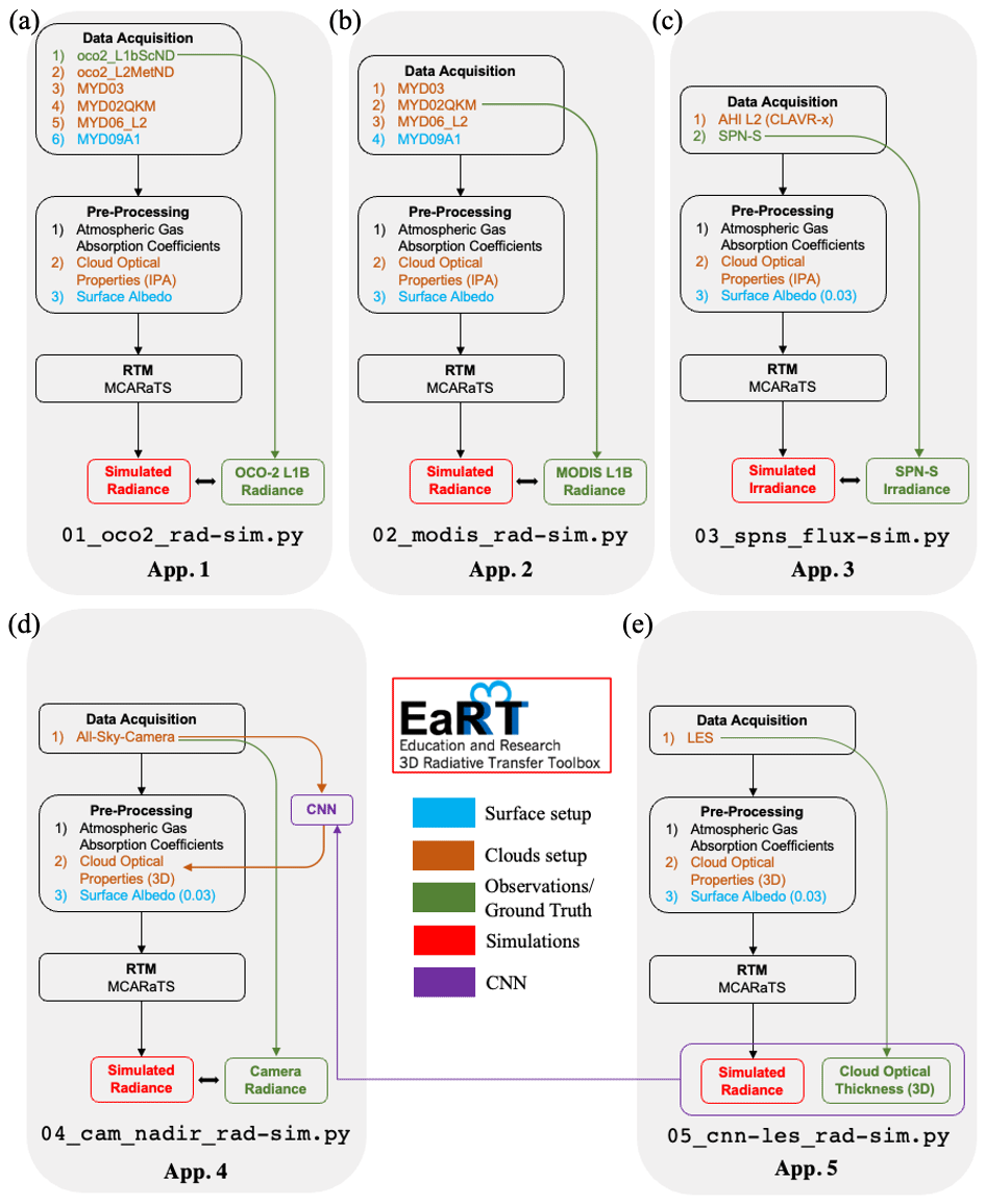
Figure 1 Flow charts of EaR³T applications for (a) OCO-2 radiance simulation at 768.52 nm (data described in Sect. 2.2.1 and 2.2.2, results discussed in Sect. 4.1), (b) MODIS radiance simulation at 650 nm (data described in Sect. 2.2.1, results discussed in Sect. 4.2), (c) SPN-S irradiance simulation at 745 nm (data described in Sect. 2.2.3 and 2.2.4, results discussed in Sect. 5), (d) all-sky camera radiance simulation at 600 nm (data described in Sect. 2.2.5, results discussed in Sect. 6), and (e) radiance simulation at 600 nm based on LES data for CNN training (Appendix B). The data products and their abbreviations are described in Sect. 2.2.

2.2 Data

The radiance simulations in App. 1 and App. 2 use data from the OCO-2 and MODIS-Aqua instruments, both of which are in a sun-synchronous polar orbit with an early afternoon Equator crossing time within NASA's A-Train satellite constellation. Figure 2 visualizes radiance measurements by OCO-2 in the context of MODIS Aqua imagery over a partially vegetated and partially cloud-covered land, illustrating that MODIS provides imagery and scene context for OCO-2, which in turn observes radiances from a narrow swath. The region is located in southwestern Colorado in the United States of America. We selected this case because both the surface and clouds are varied along with diverse surface types. The surface features green forest and brown soil, whereas clouds include small cumulus and large cumulonimbus. In addition, this scene contains relatively homogeneous cloud fields in the north and inhomogeneous cloud fields in the south, which allows us to evaluate the simulations from various aspects of cloud morphology. To simulate the radiances of both instruments we use data products from OCO-2 and MODIS, as well as reanalysis products from NASA's Global Modeling and Assimilation Office (GMAO) sampled at OCO-2 footprints and distributed along with OCO-2 data (Sect. 2.2.2).

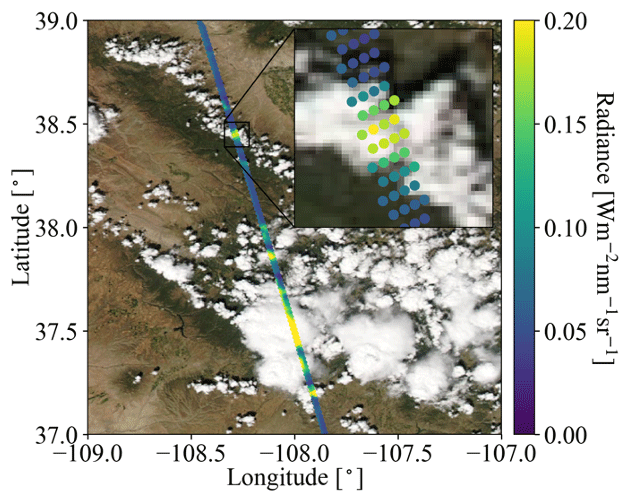
Figure 2 OCO-2-measured radiance (W m⁻² nm⁻¹ sr⁻¹) at 768.52 nm, overlaid on MODIS Aqua RGB imagery over southwestern Colorado (USA) on 2 September 2019. The inset shows an enlarged portion along the track, illustrating that OCO-2 radiances co-vary with MODIS-Aqua radiance observations (the circles are used to indicate the geolocation of OCO-2 footprints).

For App. 3 (irradiance simulations and 3D cloud bias quantification), we use geostationary imagery from the Japanese Space Agency's Advanced Himawari Imager to provide cloud information in the area of the flight path of the NASA CAMP²Ex aircraft (Reid et al., 2023). The AHI data are used in conjunction with aircraft measurements of shortwave spectral radiation (Sect. 2.2.4). Subsequently (App. 4: 3D cloud bias mitigation), we demonstrate the concept of radiance closure under partially cloudy conditions with airborne camera imagery (Sect. 2.2.5). The underlying cloud retrieval is based on a convolutional neural network (CNN), which is described in a related paper (Nataraja et al., 2022) in this special issue and relies on EaR³T-generated synthetic radiance data based on LESs.

2.2.1 Moderate Resolution Imaging Spectroradiometer (MODIS)

The MODIS instruments are multi-use multispectral radiometers onboard NASA's Terra and Aqua satellites, which were launched in 1999 and 2002, respectively. MODIS was conceived as a central element of the Earth Observing System (EOS; King and Platnick, 2018). For App. 1 and App. 2, EaR³T ingests MODIS level 1B radiance products at the 0.25 km scale (channels 1 and 2, bands centered at 650 and 860 nm), MxD02QKM, where “x” stands for “O” in the case of MODIS on Terra, and “Y” in the case of Aqua data), the geolocation product (MxD03), the level 2 cloud product (MxD06), and the surface BRDF (bidirectional reflectance distribution function) product (MCD43A3). For this paper, we mainly use Aqua data (MYD) from data collection 6.1.

For cloud properties in App. 2, we use the MODIS cloud product (MxD06L2, collection 6.1). It provides cloud properties, such as cloud optical thickness (COT), cloud-effective radius (CER), cloud thermodynamic phase, cloud top height (CTH), etc. (Nakajima and King, 1990; Platnick et al., 2003). Since 3D cloud effects such as horizontal photon transport are most significant at small spatial scales (e.g., Song et al., 2016), we use the high-resolution red (650 nm) channel 1 (250 m) and derive COT directly from the reflectance in the level 1B data (MYD02QKM) instead of using the coarser-scale operational product from MYD06. CER and CTH are sourced from MYD06 and re-gridded to 250 m. The EaR³T strategy for MODIS data is similar, in principle, to the more advanced method by Deneke et al. (2021), which uses a high-resolution wide-band visible channel from geostationary imagery to up-sample narrow-band coarse-resolution channels. However, we simplified cloud detection and COT retrieval (referred to as COT_IPA) from reflectance data for the purpose of our paper by using a threshold method (Appendix C1) and an IPA reflectance-to-COT mapping (Appendix C2). In future versions of EaR³T this will be upgraded to more sophisticated algorithms. A simple algorithm (Appendix D1) is used to correct for the parallax shift based on the sensor geometries and cloud heights. The cloud top height data are provided by the MODIS L2 cloud product, and we assume that the cloud base is the same.

For the surface albedo required by the RTM, we used MCD43A3, which provides BRDF calculated from a combination of Aqua and Terra MODIS and MISR (Multi-Angle Imaging Spectroradiometer) clear-sky observations aggregated over a 16 d period (Strahler et al., 1999). This product contains white-sky albedo (WSA, also known as bihemispherical reflectance), which is obtained by integrating the BRDF over all viewing angles (Strahler et al., 1999). The WSA is available on a sinusoidal grid with a spatial resolution of 500 m for MODIS band 2 and includes atmospheric correction for gas and aerosol scattering and absorption. Assuming a Lambertian surface in this first release of EaR³T, we used the WSA (referred to as surface albedo from now on) as surface albedo input to the RTM.

2.2.2 Orbiting Carbon Observatory 2 (OCO-2)

The OCO-2 satellite was inserted into NASA's A-Train constellation in 2014 and flies about 6 min ahead of Aqua. OCO-2 provides the column-averaged carbon dioxide (CO₂) dry-air mole fraction (XCO₂) through passive spectroscopy based on hyperspectral radiance observations in three narrow wavelength regions, the oxygen A-band (∼ 0.76 µm), the weak CO₂ band (∼ 1.60 µm), and the strong CO₂ band (∼ 2.06 µm). As shown in the inset of Fig. 2, it takes measurements in eight footprints across a narrow swath. Each of the footprints has a size around 1–2 km, and the spectra for the three bands are provided by separate, co-registered spectrometers (Crisp, 2015).

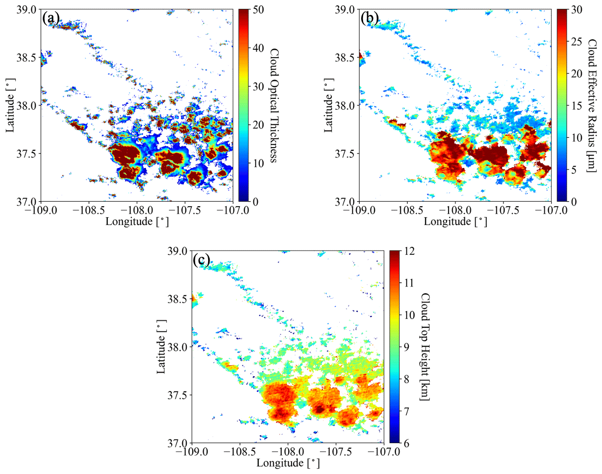
Figure 3 (a) Cloud optical thickness derived from MODIS L1B radiance at 650 nm by the IPA reflectance-to-COT mapping (Appendix C2), (b) cloud effective radius (µm), and (c) cloud top height (km) colocated from the MODIS L2 cloud product. The locations of the cloudy pixels were shifted to account for parallax and wind effects. The parallax correction ranged from near zero for low clouds and 1 km for high clouds (10 km CTH). The wind correction was around 0.8 km, given the median wind speed of 2 m s⁻¹ to the east.

The OCO-2 data products used are (1) level 1B calibrated and geolocated science radiance spectra (L1bScND), (2) standard level 2 geolocated XCO₂ retrievals results (L2StdND), and (3) meteorological parameters interpolated from GMAO (L2MetND) at OCO-2 footprint location. Since MODIS on Aqua flies over a scene 6 min after OCO-2, the clouds move with the wind over this time period. We therefore added a wind correction on top of the parallax-corrected cloud fields obtained from MODIS (Sect. 2.2.1). This was done with the 10 m wind speed data from L2MetND (see Appendix D2). For the same scene as shown in Fig. 2, Fig. 3 shows (a) COT_IPA, (b) CER, and (c) CTH, all corrected for both parallax and wind effects (these corrections are shown in Fig. A5 in Appendix D2). The parallax and wind corrections are imperfect as certain assumptions are involved. For example, they rely on the cloud top height from the MODIS cloud product. In addition, they process the whole scene with one single sensor viewing the geometry. To minimize artifacts introduced by the assumptions, one can apply the simulation to a smaller region.

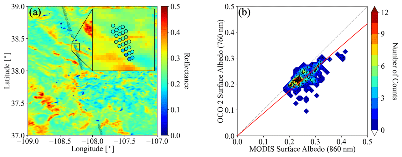
Figure 4 (a) Surface albedo from the OCO-2 L2 product in the oxygen A-band (near 760 nm), overlaid on the surface albedo from the MODIS MCD43A3 product at 860 nm. (b) OCO-2 surface albedo at 760 nm versus MODIS surface albedo at 860 nm, along with linear regression (${\mathit{\alpha }}_{\mathrm{OCO}}=c\cdot {\mathit{\alpha }}_{\mathrm{MOD}}$) as indicated by the red line (slope c = 0.867).

The OCO-2 data (L2StdND) themselves only provide sparse surface BRDF (referred to as surface albedo from now on) for the footprints that are clear, while EaR³T requires surface albedo for the whole domain. Therefore, we used MCD43A3 as a starting point. However, since MODIS does not have a channel in the oxygen A-band, MODIS band 2 (860 nm) was used as a proxy for the 760 nm OCO-2 channel as follows: we collocated the OCO-2 retrieved 760 nm surface albedo α_OCO within the corresponding 860 nm MODIS MCD43A3 data α_MOD as shown in Fig. 4a (same domain as Figs. 2 and 3) and calculated a scaling factor assuming a linear relationship between α_OCO and α_MOD (${\mathit{\alpha }}_{\mathrm{OCO}}=c\cdot {\mathit{\alpha }}_{\mathrm{MOD}}$). Figure 4b shows α_OCO versus α_MOD for all cloud-free OCO-2 footprints. The red line shows a linear regression (derived scale factor c = 0.867). Optionally, the OCO-2-scaled, MODIS-derived surface albedo fields can be replaced by the OCO-2 surface albedo products for pixels where they are available. The replacement is done for App. 1. The scaled and replaced surface albedo is then treated as input to the RTM assuming a Lambertian surface.

2.2.3 Advanced Himawari Imager (AHI)

The Advanced Himawari Imager (AHI, used for App. 3) is a payload on Himawari-8, a geostationary satellite operated by the Meteorological Satellite Center (MSC) of the Japanese Meteorological Agency. The AHI provides 16 channels of spectral radiance measurements from the shortwave (0.47 µm) to the infrared (13.3 µm). During CAMP²Ex, the NASA in-field operational team closely collaborated with the team from MSC to provide AHI satellite imagery at the highest resolution over the Philippine Sea. From the AHI imagery, the cloud product generation system - Clouds from AVHRR Extended System (CLAVR-x), was used to generate cloud products from the AHI imagery (Heidinger et al., 2014). The cloud products from CLAVR-x include cloud optical thickness, cloud effective radius, and cloud top height at 2 (at nadir) to 5 km spatial resolution. Since AHI provides continuous regional scans every 10 min, the AHI cloud product has a temporal resolution of 10 min.

2.2.4 Spectral Sunshine Pyranometer (SPN-S)

The SPN-S is a prototype spectral version of the commercially available global–diffuse SPN1 pyranometer (Wood et al., 2017; Norgren et al., 2022). The radiometer uses a seven-detector design in combination with a fixed shadow mask that enables the simultaneous measurement of both diffuse and global irradiances, from which the direct component of the global irradiance is calculated via subtraction. The detector measures spectral irradiance from 350 to 1000 nm, and the spectrum is sampled at 1 nm resolution with 1 Hz timing.

During the CAMP²Ex mission, the SPN-S was mounted to the top of the NASA P-3 aircraft, where it sampled downwelling solar irradiance. To ensure accurate measurements, pre- and post-mission laboratory-based calibrations were completed using tungsten “FEL” lamps that are traceable to a National Institute of Standards and Technology standard. Additionally, the direct and global irradiances were corrected for deviations in the SPN-S sensor plane from horizontal that are the result of changes in the aircraft's pitch or roll. This attitude correction applied to the irradiance data is a modified version of the method outlined in Long et al. (2010). However, whereas Long et al. (2010) employ a “box” flight pattern to characterize the sensor offset angles, in this study an aggregation of flight data containing aircraft heading changes under clear-sky conditions are used as a substitute. The estimated uncertainty of the SPN-S system is 6 % to 8 %, with 4 % to 6 % uncertainty stemming from the radiometric lamp calibration process, and up to another 2 % resulting from insufficient knowledge of the sensor cosine response. The stability of the system under operating conditions is 0.5 %. A thorough description of the SPN-S and its calibration and correction procedures is provided in Norgren et al. (2022). In this paper (App. 3) only the global downwelling irradiance sampled by the 745 nm channel is used.

2.2.5 Airborne All-Sky Camera (ASC)

The All-Sky Camera (used for App. 4) is a commercially available camera (ALCOR ALPHEA 6.0CW, https://www.alcor-system.com/common/allSky/docs/ALPHEA_Camera%20ALL%20SKY%20CAMERA_Doc.pdf, last access: 24 April 2022) with fish-eye optics for hemispheric imaging. It has a charge-coupled device (CCD) detector that measures radiances in red, green, and blue channels. Radiometric and geometric calibrations were performed at the Laboratory of Atmospheric and Space Physics at the University of Colorado, Boulder. The three color channels are centered at 493, 555, and 626 nm for blue, green, and red, respectively, with bandwidths of 50–100 nm. Only radiance data from the red channel are used in this paper. The spatial resolution of the ASC depends on the altitude of the aircraft and the viewing zenith angle. Across the hemispheric field of view of the camera, the resolution of the field angle is approximately constant, at about 0.09^∘. At a flight level of 5 km, this translates to a spatial resolution of 8 m at nadir. However, due to accuracy limitations of the geometric calibration and the navigational data from an inertial navigation system (INS), the nadir geolocation accuracy could only be verified to within ±50 m. During the CAMP²Ex flights, the camera exposure time was set manually to minimize saturation of the detector. The standard image frame rate is 1 Hz. The precision of the camera radiances is on the order of 1 %, and the radiometric accuracy is 6 %–7 %.

3 EaR³T procedures

In the previous section, we described the input data for the EaR³T applications. In this section, we will focus on providing the complete workflow (shown in Fig. 1) for the five applications.

After the required data files have been automatically downloaded in the data acquisition step as described in previous section, EaR³T pre-processes them and generates the optical properties of atmospheric gases, clouds, aerosols, and the surface. In Fig. 1, the mapping from input data to these properties is color-coded component-wise (brown for associated cloud property processing if available, blue for associated surface property processing if available, green for associated ground truth property). The EaR³T code base used in this paper (v0.1.1; Chen et al., 2023) only includes MCARaTS as the 3D RT solver, but others are planned for the future. MCARaTS is a radiative transfer solver that uses a Monte Carlo photon-tracing method (Iwabuchi, 2006). It outputs radiation (radiance or irradiance) based on the inputs of radiative properties of surface and atmospheric constituents (e.g., gases, aerosols, clouds) such as single-scattering albedo, scattering phase function, or asymmetry parameter, and solar- and sensor-viewing geometries. The setup of these input properties is implemented in EaR³T's pre-processing steps, which translates atmospheric properties into solver-specific input with minimum user intervention. To achieve this, EaR³T is modular so that it can be extended as new solvers are added. Although the five specific applications in this paper do not include aerosol layers, the setup of aerosol fields is fully supported and has been used in other applications (e.g., Gristey et al., 2022). After pre-processing, the optical properties are fed into the RT solver. Finally, the user obtains radiation output from EaR³T, i.e., either radiance or irradiance. The output is saved in HDF5 format and can be easily distributed and accessed by various programming languages. The data variables contained in the HDF5 output are provided in Table A2 in Appendix A1.

The processes of data acquisition, pre-processing, and RTM setup and execution (shown in Fig. 1) are automated such that the 3D-RT and 1D-RT calculations can be performed for any region at any date and time using satellite or aircraft data or other data resources such as LES. A detailed code walk-through of App. 1 and 2 is provided in Appendix A2. Since EaR³T is developed as an educational and research 3D-RT tool collection by students, it is a living code base, intended to be updated over time. The master code modules for the five applications as listed in Fig. 1 are included in the EaR³T package under the examples directory. In the current release (v0.1.1), only a limited documentation for the installation and usage, including example code for EaR³T, is provided. More effort will be dedicated toward documentation in the near-future.

In the following sections, we discuss results obtained from EaR³T, starting with those from examples/01_oco2_rad-sim.py and examples/02_modis_rad-sim.py (Sect. 4), then those from examples/03_spns_flux-sim.py (Sect. 5), and concluding with those from examples/04_cam_nadir_rad-sim.py (Sect. 6). The usage of the EaR³T package, including the technical input and output parameters and a code walk-through, is provided in Appendix A.

4 EaR³T as a 3D satellite radiance simulator

This section demonstrates the automated 3D radiance simulation for satellite instruments by EaR³T for measured OCO-2 and MODIS radiance based on publicly available MODIS retrieval products. The OCO-2 application is an example of radiance consistency between two distinct satellite instruments where the measurements of one (here, OCO-2) are compared with the simulations based on data products from the other (here, MODIS). The MODIS application, on the other hand, is an example of radiance self-consistency. We will show how inconsistencies can be used for detecting cloud and surface property retrieval biases.

4.1 OCO-2 (App. 1)

The OCO-2 radiance measurements at 768.52 nm for our sample scene in the context of MODIS imagery are shown in Fig. 2. For that track segment, Fig. 5a shows the simulated radiance and the measurements as a function of latitude. The radiance was averaged over every 0.01^∘ latitude window from 37 to 39^∘ N (the standard deviation within the bin indicated by the shaded color). In clear-sky regions (e.g., around 38.2^∘ N), the 3D simulations (red) are systematically higher than the measurements (black), even though the footprint-level OCO-2 surface albedo retrieval was used to replace and scale the MCD43 surface albedo field as described in Sect. 2.2.2 (Fig. 4). This is probably because, unlike the MCD43 algorithm which relies on multiple overpasses and multiple days for cloud-clearing, the OCO-2 retrieval is done for any clear footprint. Clouds in the vicinity lead to enhanced diffuse illumination that is erroneously attributed to the surface albedo itself. The EaR³T IPA calculations of the clear-sky pixels (blue) essentially reverse the 3D effect and therefore match the observations better. The 3D calculations enhance the reflectance through the very same 3D cloud effects that led to the enhanced surface illumination in the first place. It is possible to correct this effect by downscaling the surface albedo according to the ratio between clear-sky 3D and IPA calculations, but this process is currently not automated.

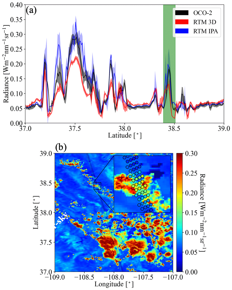
Figure 5 (a) Latitudinally averaged (0.01^∘ spacing) radiance calculations from EaR³T (red: 3D; blue: IPA) and OCO-2 measured radiance at 768.52 nm (black) The green shaded area indicates the inset shown in (b). (b) The same as Fig. 2 except OCO-2 measured radiance overlaid on IPA radiance simulations at 768.52 nm. The solar zenith angle (SZA) for the radiance simulation case is 34.3^∘.

In the cloudy locations (radiance value greater than ∼ 0.05), the IPA calculations match the OCO-2 observations on a footprint-by-footprint level (see Fig. 5b), demonstrating that wind and parallax corrections were performed successfully. Of course, there is not always a perfect agreement because of morphological changes in the cloud field over the course of 6 min. It is, however, apparent that the 3D calculations agree to a much lesser extent with the observations than the IPA calculations. Just like the mismatch for the clear-sky pixels indicates a bias in the input surface albedo, the bias here means that the input cloud properties (most importantly COT) are inaccurate. For most of the reflectance peaks, the 3D simulations are too low, which means that the input COT is biased low. This is due to 3D cloud effects on the MODIS-based cloud retrieval. Since they are done with IPA, any net horizontal photon transport is not considered, which leads to an apparent surface brightening as noted above at the expense of the cloud brightness. As a result, the COT from darker clouds is significantly underestimated. This commonly known problem (Barker and Liu, 1995), with several aspects discussed in the subsequent EaR³T applications, can be identified by radiance consistency checks such as the one shown in Fig. 5 and mitigated by novel types of cloud retrievals that do take horizontal photon transport into account (Sect. 6).

4.2 MODIS (App. 2)

To go beyond the OCO-2 track and understand the bias between simulated and observed radiances from a domain perspective, we now consider the radiance simulations for the MODIS 650 nm channel. The setup is exactly the same as for the OCO-2 simulations, except that (1) the viewing zenith angle is set to the average viewing zenith angle of MODIS within the shown domain (instead of OCO-2) and (2) the surface albedo (or WSA) from MCD43 is used directly, this time from the 650 nm channel without rescaling. Figure 6a shows the MODIS-measured radiance field, while Fig. 6b shows the EaR³T 3D simulations. Visually, the clouds from the EaR³T simulation are generally darker than the observed clouds, which is in line with our aforementioned explanation of net horizontal photon transport. They are also blurrier because radiative smoothing (Marshak et al., 1995) propagates into the retrieved COT fields, which are subsequently used as input to EaR³T. The IPA RT calculations agree with the observations for clouds (see Fig. A4a in Appendix C2), which is expected as the IPA calculations and retrievals go through the same RT process, and the darkening and smoothing effects (referred to as 3D effects) are due to horizontal photon transport. To look at the 3D effects more quantitatively, Fig. 7 shows a heatmap plot of simulated radiance versus observed radiance. It shows that the radiance for cloud-covered pixels (labeled “cloudy”) from EaR³T are mostly biased low, while good agreement between simulations and observations was achieved for clear-sky radiance (labeled “clear-sky”). The good agreement over clear-sky regions is expected. As mentioned above, we use MCD43 as surface albedo input, which in contrast to the OCO-2 surface albedo product is appropriately cloud-screened and therefore does not have a high reflectance bias. There is, of course, a reflectance enhancement in the vicinity of clouds, but it is captured by the EaR³T calculations. The fact that the calculations agree with the observations even for clear-sky pixels in the vicinity of clouds shows that the concept of radiance consistency works to ensure correct satellite retrievals even in the presence of clouds. It also corroborates our observation from Sect. 4.1 that COT_IPA is biased low. Since the MODIS reflectance is not self-consistent with respect to 3D RT calculations using COT_IPA as shown for the cloudy pixels in Fig. 7, we can identify a bias in the cloud properties even without knowing the ground truth of COT. On the other hand, successful closure in radiance (self-consistency) would provide an indication that the input fields including COT are accurate, although it is certainly a weaker metric than direct verification of the retrievals through aircraft–satellite retrieval validation using observations from in situ instruments.

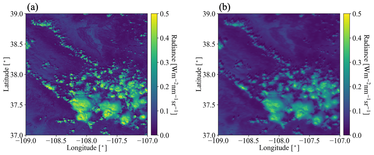
Figure 6 (a) MODIS-measured radiance in channel 1 (650 nm). (b) Simulated 3D radiance at 650 nm from EaR³T. The solar zenith angle for the radiance simulation case is 34.94^∘.

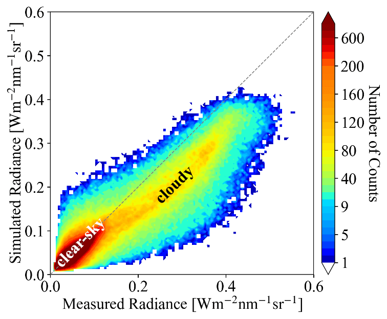
Figure 7 Heatmap plot of EaR³T simulated 3D radiance versus MODIS measured radiance at 650 nm.

Summarizing the two satellite radiance simulator applications, one can say that EaR³T enables a radiance consistency check for inhomogeneous cloud scenes. We demonstrated that a lack of simulation–observation consistency (MODIS versus OCO-2) and self-consistency (MODIS versus MODIS) can be traced back to biased surface albedo or cloud fields in the simulator input. This can become a diagnostic tool for the quality of retrieval products from future or current missions, even when the ground truth is not known. Although not shown, the errors in the simulated radiance associated with the fixed-SZA (solar zenith angle) assumption (domain average) are negligible. However, the vertical extent of the clouds affects the simulated radiance – the larger the vertical extent, the larger the 3D effects (more horizontal photon transport). Since we assume (1) a cloud geometric thickness of 1 km for clouds with CTH less than 4 km and (2) a cloud base height of 3 km for clouds with CTH greater than 4 km, the simulated radiance at the satellite sensor level is valid for that proxy cloud only. For clouds that are geometrically thicker than the assumed cloud geometrical thickness, the simulated radiance would be even lower due to enhanced horizontal photon transport. Either way, the comparison with the actual radiance measurements will reveal a lack of closure. Additionally, although the clouds introduce the lion's share of the 3D bias that is identified by the radiance consistency check, additional discrepancies can be introduced in different ways. For example, the topography (mountainous region in Colorado) is not considered by MCARaTS (it is considered by MYSTIC, but this solver has not been implemented yet).

For reference, in term of simulation running time, the MODIS simulation (domain size of [​​​​​​​N_x = 846; N_y = 846]) took about 15 min on a Linux workstation with eight CPUs for three 3D RT runs with 10⁸ photons. With a slightly modified setup and parallelization, the automation can be easily applied for entire satellite orbits, although more research is required to optimize the computation speed depending on the desired output accuracy.

5 EaR³T as 3D aircraft irradiance simulator (App. 3)

In contrast to the previous applications that focused on satellite remote sensing, we will now be applying EaR³T to quantify 3D cloud retrieval biases through direct, systematic validation of imagery-derived irradiances against aircraft measurements, instead of using the indirect path of radiance consistency in Sect. 4. Previous studies (e.g., Schmidt et al., 2007; Kindel et al., 2010) conducted radiative closure between remote-sensing-derived and measured irradiance using isolated flight legs as case studies. Here, with the efficiency afforded by the automated nature of EaR³T, we are able to conduct radiative closure of irradiance through a statistical approach that employs campaign-scale amounts of measurement data. Specifically, we used EaR³T to perform large-scale downwelling irradiance simulations at 745 nm based on geostationary cloud retrievals from AHI for the CAMP²Ex campaign, and directly compare these simulations to the SPN-S measured irradiances onboard the P-3 aircraft. This is done for all below-cloud legs from the entire campaign with the aim of assessing the degree to which satellite-derived near-surface irradiances reproduce the true conditions below clouds.

The irradiance simulation process is similar to the previously described radiance simulation in Sect. 4, with only a few modifications. First, we used cloud optical properties from the AHI cloud product (COT, CER, and CTH) as direct inputs into EaR³T. Secondly, we used a constant ocean surface albedo value of 0.03. Such simplification in surface albedo is made under the assumption that (1) the ocean surface is calm with no whitecaps and that (2) the Lambertian BRDF is sufficient (instead of directionally dependent BRDF) to represent surface albedo for the irradiance calculation. Since the ocean surface albedo can greatly differ from 0.03 when the sun is extremely low (Li et al., 2006), we excluded data under low-sun conditions where the SZA is greater than 45^∘. Lastly, since EaR³T can only perform 3D simulations for a domain at a single specified solar geometry, we divided each CAMP²Ex research flight into small flight track segments where each segment contains 6 min of flight time. The size and shape of the flight track segments can vary significantly due to the aircraft maneuvers, aircraft direction, aircraft speed, etc. For each flight track segment, EaR³T performs irradiance simulations for a domain that extends half a degree at an averaged solar zenith angle. In contrast to the radiance simulation, which has two-dimensional output at a specified altitude and sensor geometry, the irradiance simulation provides three-dimensional output. In addition to x (longitude) and y (latitude) vectors, it has a vertical dimension along z (altitude). From the simulated three-dimensional irradiance field, the irradiance for the flight track segment is linearly interpolated to the x–y–z location (longitude, latitude, and altitude) of the aircraft. EaR³T automatically subdivides the flight track into tiles encompassing track segments and extracts the necessary information from the aircraft navigational data. Based on the aircraft time and position, EaR³T downloads the AHI cloud product that is closest in time and space to the domain containing the flight track segment.

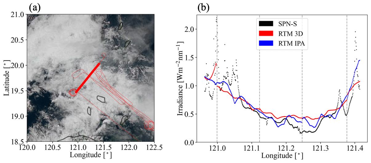
Figure 8 (a) Flight track overlay HIMAWARI AHI RGB imagery over the Philippine Sea on 20 September 2019. The thin line shows the entire flight track within the domain. The thick line highlights the specific leg analyzed in (b). (b) Measured downwelling irradiance from SPN-S at 745 nm and calculated 3D and IPA irradiance from EaR³T for the highlighted flight track in (a).

Figure 8 shows the simulated irradiance for a sample flight track below clouds on 20 September 2019. Figure 8a shows the flight track overlaid on AHI imagery. Figure 8b shows 3D (in red) and IPA (in blue) downwelling irradiance simulations for the highlighted flight track in Fig. 8a, as well as measurements by the SPN-S (in black). Since the 3D and IPA simulations are performed separately at discrete solar and sensor geometries for each flight track segment based on potentially changing cloud fields from one geostationary satellite image to the next, discontinuities in the calculations (indicated by dashed gray lines) are expected. The diffuse irradiance (downwelling and upwelling) can also be simulated and compared with radiometer measurements (not shown here). Since the irradiance was simulated and measured below clouds, high values of downwelling irradiance indicate thin-cloud or cloud-free regions, while low values of downwelling irradiance indicate thick-cloud regions. The simulations successfully captured this general behavior – clouds thickened from west to east until around 121.25^∘ E and thinned eastwards. However, the fine-scale variabilities in irradiance were not captured by the simulations due to the coarse resolution of COT in the AHI cloud product (3–5 km). Additionally, the simulations also missed the clear-sky regions in the very east and west of the flight track, as indicated by high downwelling irradiance values measured by SPN-S. This is probably also due to the coarse resolution of the AHI COT product where small cloud gaps are not represented. Large discrepancies between simulations and observations occur in the midsection of the flight track where clouds are present (e.g., longitude range from 121.15 to 121.3^∘). Although the 3D calculations differ somewhat from the IPA results, they are both biased high, likely because the input COT (the IPA-retrieved AHI product) is biased low. This bias is caused by the same mechanism that was discussed earlier in the MODIS examples (Sect. 4.2). This begs the question as to whether this is true for the entire field mission. To answer the question, we performed a systematic comparison of the cloud transmittance for all available below-cloud flight tracks from CAMP²Ex, using EaR³T's automated processing pipeline. The output of this pipeline is visualized in time-synchronized flight videos (Chen et al., 2022), which show the simulations and observations along all flight legs point by point. These videos give a glimpse of the general cloud environment during the field campaign from the geostationary satellite perspective.

For this comparison, we use transmittance instead of irradiance. The transmittance is calculated by dividing the downwelling irradiance below clouds ($F_{\downarrow }^{\mathrm{bottom}}$) by the downwelling irradiance at the top of the atmosphere extracted from the Kurucz solar spectra ($F_{\downarrow }^{\mathrm{TOA}}$; Kurucz, 1992) at incident SZA, where

$$\begin{array}{}\text{(1)}& \mathrm{Transmittance}={\displaystyle \frac{F_{\downarrow }^{\mathrm{bottom}}}{F_{\downarrow }^{\mathrm{TOA}}\cdot \cos \left(\mathrm{SZA}\right)}}.\end{array}$$

Thus, the transmittance has less diurnal dependence than the irradiance. Figure 9 shows the histograms of the simulated and measured cloud transmittance from all below-cloud legs. The average values are indicated by dashed lines. Although the averaged values of IPA and 3D transmittance are close, their distributions are different. Only the 3D calculations and the measured transmittance reach values beyond 1. This occurs in clear-sky regions in the vicinity of clouds that receive photons scattered by the clouds, as previously discussed for the OCO-2 application.

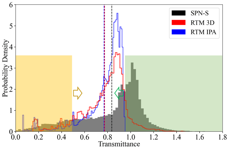
Figure 9 Histogram of measured transmittance from SPN-S at 745 nm (dark gray filled area) and calculated 3D (solid red line) and IPA (solid blue line) transmittance from EaR³T for all the below-cloud flight tracks during CAMP²Ex in 2019. The mean values are indicated by dashed lines. The yellow-shaded (green-shaded) area represents the relatively low (high) transmittance region where the probability density of the observed transmittance (dark gray filled area) is greater than the calculations.

Both the distribution and the mean value of the simulations are different from the observations. The simulation histograms peak at around 0.9, while the observation histogram peaks at around 1. The histograms indicate that the RT simulations miss most of the clear-sky conditions because of the coarse resolution of the AHI cloud product. If clouds underfill a pixel, AHI interprets the pixel as cloudy in most cases. This leads to an underestimation of clear-sky regions as cumulus and high cirrus were ubiquitous during CAMP²Ex. The area on the left (highlighted in yellow) has low cloud transmittance associated with thick clouds. In this range, the histograms of the calculations are generally below the observations, and the probability density function (PDF) of the calculations is offset to the right (indicated by the yellow arrow). This means that the transmittance is overestimated by both IPA and 3D RT, and thus the COT of thick clouds is underestimated, consistent with what we found before (Fig. 8b). The high-biased transmittance below cloud is also consistent with the findings of low-biased reflectance (App. 1 and 2), both indicating COT of the optically thick clouds are biased low. The high-transmittance end (highlighted in green) is associated with clear-sky and thin clouds. Here, the peak of the PDF is shifted to the left (green arrow), and the calculations are biased low. This is caused by a combination of (1) the overestimation in COT of thin clouds due a 3D bias in the AHI IPA retrieval, (2) the aforementioned resolution effect that underestimates the occurrence of clear-sky regions (or overestimation in cloud fraction), and (3) net horizontal photon transport from clouds into clear-sky pixels. Overall, the calculations underestimate the true transmittance by 10 %. This might seem to contradict Fig. 7, where the calculated reflected radiance was biased low due to the underestimation of COT in the heritage retrievals, which would correspond to an overestimation of the radiation transmitted by clouds. This effect is indeed apparent in the yellow-shaded area of Fig. 9 (high COTs), but the means (dashed lines) show exactly the opposite. To understand that, one has to consider that the histogram depicts all-sky conditions, which include both cloudy and clear pixels. In this case, the direction of the overall (all-sky) bias follows the direction of the thin-cloud or clear bias, rather than the direction of the thick cloud bias. For different study regions of the globe with different cloud fractions, cloud size distributions, and possibly different imager resolutions, the direction and magnitude of the bias might be very different.

Summarizing, this application demonstrates that the EaR³T's automation feature allows systematic simulation-to-observation comparisons. If aircraft observations are available, then closure between satellite-derived irradiance and suborbital measurements is a more powerful verification of satellite cloud retrieval products than the radiance consistency from the earlier standalone satellite applications. Even more powerful is the new approach to process the data from an entire field mission for assessing the quality of cloud products in a region of interest (in this case, the CAMP²Ex area of operation).

6 EaR³T for mitigating 3D cloud retrieval biases (App. 4)

In this section, we will use high-resolution imagery from a radiometrically calibrated all-sky camera flown during the CAMP²Ex to isolate the 3D bias (sometimes referred to as IPA bias) and explore its mitigation with a newly developed CNN cloud retrieval framework (Nataraja et al., 2022). The CNN, unlike IPA, takes pixel-to-pixel net horizontal photon transport into account. It exploits the spatial context of pixels in cloud radiance imagery and extracts a higher-dimensional, multi-scale representation of the radiance to retrieve COT fields as the output. It does so by learning on “training data”, which in this case was input radiance and COT pairs synthetically generated by EaR³T using LES data from the Sulu Sea. The best CNN model, trained on different coarsened resolutions of the data pairs, is included within the EaR³T repository. For App. 4, this CNN is applied to real imagery data for the first time, which in our case are near-nadir observations by the all-sky camera (Sect. 2.2.5) that flew in CAMP²Ex.

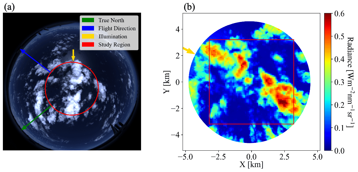
Figure 10 (a) RGB imagery of nadir-viewing all-sky camera deployed during CAMP²Ex for a cloud scene centered at 15.2744^∘ N, 123.392^∘ E over the Philippine Sea at 02:10:06 UTC on 5 October 2019. The arrows indicate true north (green), flight direction (blue), and illumination (where the sunlight comes from, yellow). (b) Red-channel radiance measured by the camera for the circular area indicated by the red circle in (a). The region in the red square shows a gridded radiance with a pixel size of 64 × 64 and spatial resolution of 100 m.

The CNN model was trained at a single (fixed) sun-sensor geometry (SZA of 29.2^∘, solar azimuth angle (SAA) of 323.8^∘, and viewing zenith angle (VZA) of 0^∘) at a spatial resolution of 100 m. We therefore chose a camera scene with a matching SZA (28.9^∘), rotated the radiance imagery to match SAA of 323.8^∘, and subsequently gridded the 8–12 m native resolution camera data to 100 m. Figure 10a shows the RGB imagery captured by the all-sky camera over the Philippine Sea at 02:10:06 UTC on 5 October 2019. The sun is located to the southeast (as indicated by the yellow arrow) and can be easily identified from the sun glint. Note that this image has not yet been geolocated; it is depicted as acquired in the aircraft reference frame. Figure 10b shows the rotated scene of the red-channel radiance for the region encircled in yellow in Fig. 10a. The sun (as indicated by the yellow arrow) is now at a SAA of 323.8^∘. The selected study region is indicated by the red square in Fig. 10b (6.4 × 6.4 km²), where the raw radiance of the camera is gridded at 100 m resolution to match the spatial resolution of the training data set of the CNN.

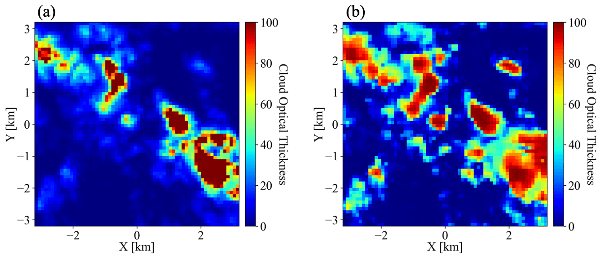
Figure 11 Cloud optical thickness for the gridded radiance in Fig. 10b (a) estimated by IPA method and (b) predicted by CNN.

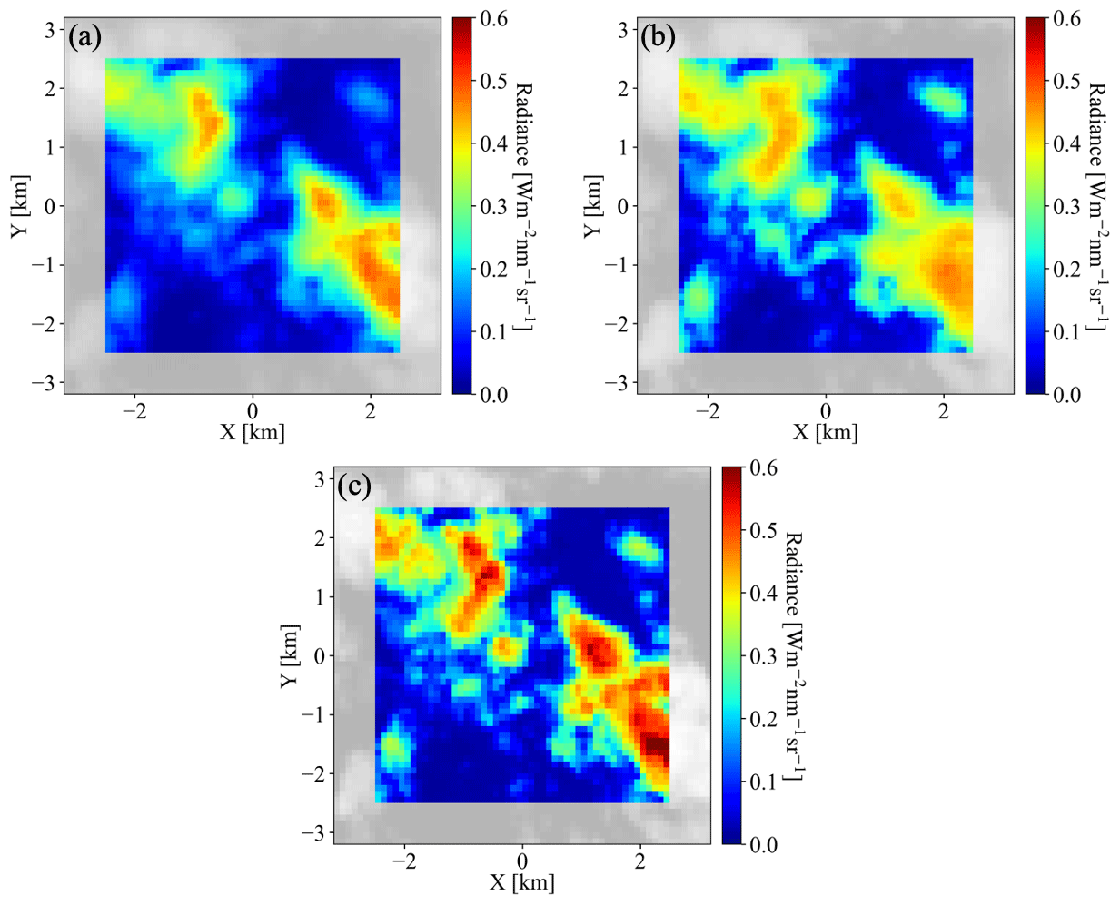
Figure 12 The 3D radiance calculations from EaR³T at 600 nm based on cloud optical thickness field (a) estimated by IPA and (b) predicted by the CNN. The radiance measured by the all-sky camera (the same as Fig. 10b) is provided in the same format in (c) for comparison. The calculations were originally performed for the 64 × 64 domain. Then seven pixels along each side of the domain (contoured in gray) were excluded, which resulted in a 50 × 50 domain.

From the radiance field, we used both the traditional IPA (based on the IPA reflectance-to-COT mapping) and the new CNN to retrieve COT fields. Figure 11 shows the COT_IPA and COT_CNN fields, which are visually quite different. For relatively thin clouds (e.g., at around {2,1.8}), the CNN tends to retrieve larger COT values than COT_IPA. Also, it returns more spatial structure than the IPA (e.g., around $\mathit{\{}\mathrm{2},-\mathrm{1}\mathit{\}}$). To assess how either retrieval performs, we now apply the radiance self-consistency approach introduced with MODIS data in Sect. 4.2. Using both the IPA and the CNN retrieval as input, we had EaR³T calculate the (synthetic) radiance that the camera should have observed if the retrieval were accurate. The clouds are assumed to be located at 1–2 km. Such an assumption is inferred from low-level aircraft observations of clouds on the same day. These radiance fields are shown in Fig. 12a and b and can be compared to Fig. 12c. Seven edge pixels have been removed from the original domain because the CNN performs poorly at edge pixels and because the 3D calculations use periodic boundary conditions.

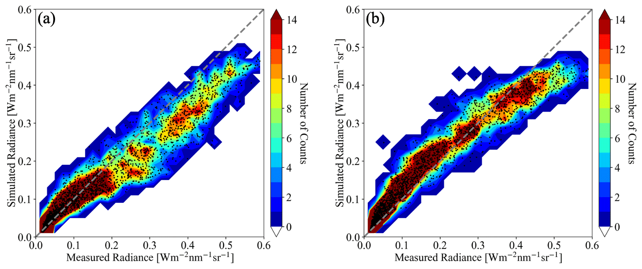
Figure 13 Scatter plot superimposed over a 2D histogram of 3D radiance calculations at 600 nm based on cloud optical thickness (a) estimated by IPA and (b) predicted by the CNN versus measured red-channel radiance from all-sky camera.

As evident from the brightest pixels in Fig. 12b and c, the radiances simulated on the basis of the COT_CNN input are markedly lower than those actually observed by the camera. This is because the CNN was trained on a LES data set with limited COT range that excluded the largest COT that occurred in practice. This means that the observational data went beyond the original training envelope of the CNN, which highlights the importance of choosing the CNN training data carefully for a given region. In Fig. 13, the simulations are directly compared with the original observations, confirming that the CNN-generated data are indeed below the observations on the high radiance end. Otherwise, the CNN-generated radiances agree with the observations. In contrast, the IPA-generated data are biased high for the optically very thin clouds (radiance below 0.1) and systematically biased low for the thick clouds (radiance above 0.2) when compared with the observations, over the dynamic range of the COT, which is indicative of the 3D retrieval bias that we discussed earlier. A small high bias occurs in the COT_CNN-based radiance simulations for the optically thin clouds (radiance value below 0.2). This probably because the CNN training as described by Nataraja et al. (2022) is (1) based on a surface albedo of zero and (2) aerosol-free atmospheric environment (an aerosol-free setup for radiance simulations is also shown in Fig. 13), where in reality the ocean is slightly brighter and atmosphere is mixed with aerosols. Here the radiance self-consistency approach again proves useful despite the absence of ground truth data for the COT. This is valuable because in reality satellite remote sensing does not have the ground truth of COT, whereas radiance measurements are always available. For the CNN, the self-consistency of the radiance is remarkable for most of the clouds (radiance smaller than 0.4), which encompass 86.8 % of the total number of image pixels.

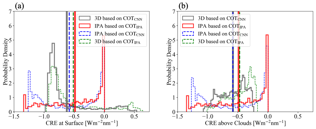
Figure 14 Histograms of cloud radiative effects derived from 3D irradiance calculations based on COT_CNN (solid gray), IPA irradiance calculations based on COT_IPA (solid red), IPA irradiance calculations based on COT_CNN (dashed blue), and 3D irradiance calculations based on COT_IPA (dashed green) both (a) at the surface and (b) above the clouds. The mean values are indicated by vertical lines.

Finally, we use EaR³T to propagate the 3D cloud retrieval bias into the associated bias in estimating the cloud radiative effect from passive imagery retrievals, which means that we are returning from a remote sensing to an energy perspective (irradiance) at the end of the paper. The calculated cloud radiative effects (CRE) of below-cloud (at the surface) and above-cloud (at 2.5 km) regions are shown in Fig. 14a and b, respectively. The most important histograms are those from 3D irradiance calculations based on the CNN retrievals (solid gray line), as this combination would be used in a next-generation framework for deriving CRE from passive remote sensing, and the other important example would be IPA irradiance calculations based on the IPA retrieval (solid red line), as done in the traditional (heritage) approach. The dashed lines are the other combinations. The mean values (red versus gray) indicate that in our case the traditional approach would lead to a high bias of more than 28 % at the surface and 20 % above clouds due to low-biased COT_IPA (consistent with findings of low-biased COT_IPA-derived reflectance from Apps. 1 and 2 and high-biased COT_IPA-derived transmittance from App. 3). Here 3D biases again do not cancel each other out in the domain average. If the CNN had better fidelity even for optically thick clouds, the real bias in CRE would be even larger. A minor but interesting finding is that regardless of which COT retrieval is used, the mean CRE is similar for IPA and 3D irradiance calculations (e.g., $\stackrel{\mathrm{‾}}{{\mathrm{CRE}}_{\mathrm{IPA}}\left({\mathrm{COT}}_{\mathrm{CNN}}\right)}\approx \stackrel{\mathrm{‾}}{{\mathrm{CRE}}_{\mathrm{3}\mathrm{D}}\left({\mathrm{COT}}_{\mathrm{CNN}}\right)}$, vertical dashed blue line locates near the vertical solid gray line) even though the PDFs are different. By far the largest impact on accuracy comes from the retrieval technique, not from the subsequent CRE calculations. Here the self-consistency check again turns out to be a powerful metric to assess retrieval accuracy. Of course, we only used a single case in this part of the paper. For future evaluation of the CNN versus the IPA, one would need to process larger quantities of data in an automated fashion, as was done in the first part of the paper. This is beyond the scope of this introductory paper and will be included in future releases of EaR³T and the CNN.

7 Summary and conclusion

In this paper, we introduced EaR³T, a toolbox that provides high-level interfaces to automate and facilitate 1D-RT and 3D-RT calculations. We presented applications that used EaR³T to perform the following tasks:

• a.

  to build a processing pipeline that can automatically simulate 3D radiance fields for satellite instruments (currently OCO-2 and MODIS) from publicly available satellite surface and cloud products at any given time over any specific region;

• b.

  to build a processing pipeline that can automatically simulate irradiance along all flight legs of aircraft missions, based on geostationary cloud products;

• c.

  to simulate radiance and irradiance for high-resolution COT fields retrieved from an airborne camera using both a traditional 1D-RT (IPA) approach and a newly developed 3D-RT (CNN) approach that considers the spatial context of a pixel.

Unlike other satellite simulators that employ 1D-RT, EaR³T is capable of performing the radiance and irradiance calculations in 3D-RT mode. Optionally, it can be turned off to link back to traditional 1D-RT codes and to calculate 3D perturbations by considering the changes in 3D-RT fields relative to the 1D-RT baseline.

With the processing pipeline referred to in task (a) above (App. 1 and App. 2, Sect. 4), we prototyped a 3D-RT-powered radiance loop (we call it “radiance self-consistency”) that is envisioned for upcoming satellite missions such as EarthCARE and AOS. Retrieved cloud fields (in our case, from MODIS and from an airborne camera) are fed back into a 3D-RT simulation engine to calculate at-sensor radiances, which are then compared with the original measurements. Beyond currently included sensors, others can be added easily, taking advantage of the modular design of EaR³T. This radiance closure loop facilitates the evaluation of passive imagery products, especially under spatially inhomogeneous cloud conditions. The automation of EaR³T permits calculations at any time and over any given region, and statistics can be built by looping over entire orbits as necessary. The concept of radiance self-consistency could be valuable even for existing imagery data sets because it allows the automated quantification of 3D-RT biases even without ground truth such as airborne irradiance from suborbital activities. Also, it can be easily extended to spectral or multi-angle observations as available from MODIS and MISR (Multi-Angle Imaging Spectroradiometer), thus providing more powerful constraints to the remote sensing products. In the future it should be possible to include a 3D-RT pipeline such as EaR³T into operational processing of satellite derived data products.

Benefitting from the automation of EaR³T in task (b) above (App. 3, Sect. 5), we performed 3D-RT irradiance calculations for the entire CAMP²Ex field campaign, moving well beyond radiation closure case studies, and instead we systematically evaluated satellite-derived radiation fields with aircraft data for an entire region. From the comparison based on all below-cloud flight tracks during the entire campaign, we found that the satellite-derived cloud transmittance was biased low by 10 % compared to the observations when relying on the heritage satellite cloud product.

From the statistical results of the CAMP²Ex irradiance closure in task (b), we concluded that the bias between satellite-derived irradiances and the ground truth from aircraft measurements was due to a combination of the coarse spatial resolution of the geostationary imagery products and 3D-RT effects. To minimize the coarse-resolution part of the bias and thus to isolate the 3D-RT bias, we used high-resolution airborne camera imagery in task (c) (App. 4, Sect. 6) and found that biases persisted even with increased imager resolution. The at-sensor radiance derived from COT_IPA was inconsistent with the original measurements. For cloudy pixels, the calculated radiance was well below the observations, confirming an overall low bias in COT_IPA. This low bias could be largely mitigated with the context-aware CNN developed separately in Nataraja et al. (2022) and included in EaR³T. Of course, this novel technique has limitations. For example, the camera reflectance data went beyond the CNN training envelope, which would need to be extended to larger COT values in the future. In addition, the CNN only reproduces two-dimensional cloud fields and does not provide access to the vertical dimension, which will be the next frontier to tackle. Still, the greatly improved radiance consistency from COT_IPA to COT_CNN indicates that the EaR³T–LES–CNN approach shows great promise for the mitigation of 3D-RT biases associated with heritage cloud retrievals. We also discovered that for this particular case, the CRE calculated from traditional 1D cloud products can introduce a warm bias of at least 28 % at the surface and 20 % above clouds.

EaR³T has proven to be capable of facilitating 3D-RT calculations for both remote sensing and radiative energy studies. Beyond the applications described in this paper, EaR³T has already been extensively used by a series of ongoing research projects for tasks such as producing massive 3D-RT calculations as training data for a new generation of CNN models (Nataraja et al., 2022), evaluating 3D cloud radiative effects associated with aerosols (Gristey et al., 2022), and creating flight track and satellite track simulations for mission planning. More importantly, the strategies provided in this paper put novel machine learning algorithms on a physical footing, opening the door for the mitigation of complexity-induced biases in the near future. More development effort will be invested into EaR³T in the future, with the goals of minimizing the barriers to using 3D-RT calculations and promoting 3D cloud studies. EaR³T will continue to be an educational tool driven by graduate students. In the future, we plan to add support for additional publicly available 3D RT solvers, e.g., SHDOM (Spherical Harmonic Discrete Ordinate Method; Evans, 1998; Pincus and Evans, 2009), as well as built-in support for HITRAN and associated correlated-k methods (currently, we are implementing such an approach for the longwave wavelength range). From a research perspective, we anticipate that EaR³T will enable the systematic quantification and mitigation of 3D-RT biases of imagery-derived cloud–aerosol radiative effects and may be the starting point for operational use of 3D-RT for future satellite missions.

Appendix A

A1 Technical input and output parameters of EaR³T

EaR³T provides various functions that can be combined to tailored pipelines for automatic 3D radiative transfer (3D-RT) calculations as described in this paper (App. 1–5), as well as for complex research projects beyond. Since EaR³T is written in Python, the modules and functions can be integrated into existing functions developed by the users themselves. Parallelization is enabled in EaR³T by default through multi-processing to accelerate computations. If multiple CPUs are available, EaR³T will distribute jobs for the 3D RT calculations. By default, the maximum number of CPUs will be used. Since EaR³T is designed to make the process of setting up and running 3D-RT calculations simple, some parameters that are unavailable from the input data but are required by the RT solvers are populated via default values and assumptions. However, this does not mean that by using EaR³T one must use these assumptions; they can be easily superseded by user-provided settings. To facilitate this process, Table A1 provides a detailed list of parameters (subject to change in future updates) that can be controlled and modified by the user. In examples/02_modis_rad-sim.py, we defined these user-controllable parameters as global variables for providing easy access to the user. In the future, most of the parameters will be controllable through a dedicated configuration file for optimal transparency. These parameters can be changed within the code. For instance, by changing the parameters of “date” (Line 67 in examples/02_modis_rad-sim.py) and “region” (Line 68 in examples/02_modis_rad-sim.py) within “params” into the following form:

params['date'] = datetime.datetime(2022, 2, 10)
params['region'] = [-6.8, -2.8, 17.0, 21.0]

one can perform similar RT calculations (as demonstrated in App. 2) for another date and region of interest (here, the western Sahara on 10 February 2022). Note that as the code is under active development, the line numbers are only valid in the version release of v0.1.1 and might change in the future. Given the input parameters, EaR³T will calculate radiance or irradiance and save the calculations into a HDF5 (hierarchical data format version 5) file. The output data variables are provided in Table A2.

Table A1 List of parameters used in the five applications. The line numbers used in the table are referring to the code script of each application. If two line numbers are provided, the first one indicates where the parameter is defined and the second one indicates where the parameter is passed into the radiative transfer setup. Users can change either one for customization purposes. NA​​​​​​​: not available.

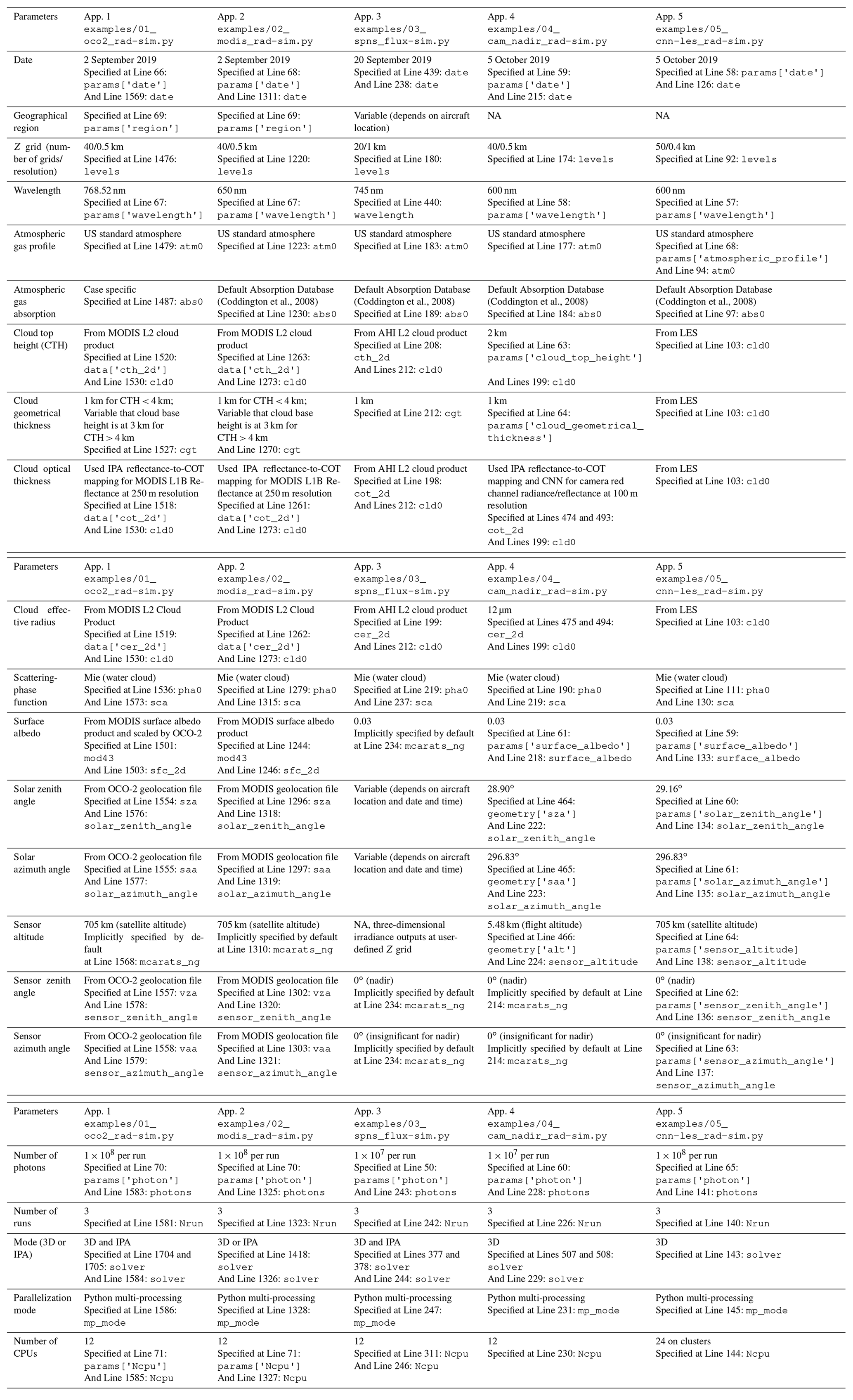
Table A2 Data variables contained in the output HDF5 file from EaR³T for radiance and irradiance calculations. The radiance is simulated with a user-specified sensor geometry at a given altitude using forward photon tracing. The data variables listed under “metadata” are included for both radiance and irradiance calculations. N_x, N_y, and N_z​​​​​​​ are the number of pixels along x, y, and z direction, respectively. N_g is the number of g, as explained in Appendix A2. NA​​​​​​​: not available.

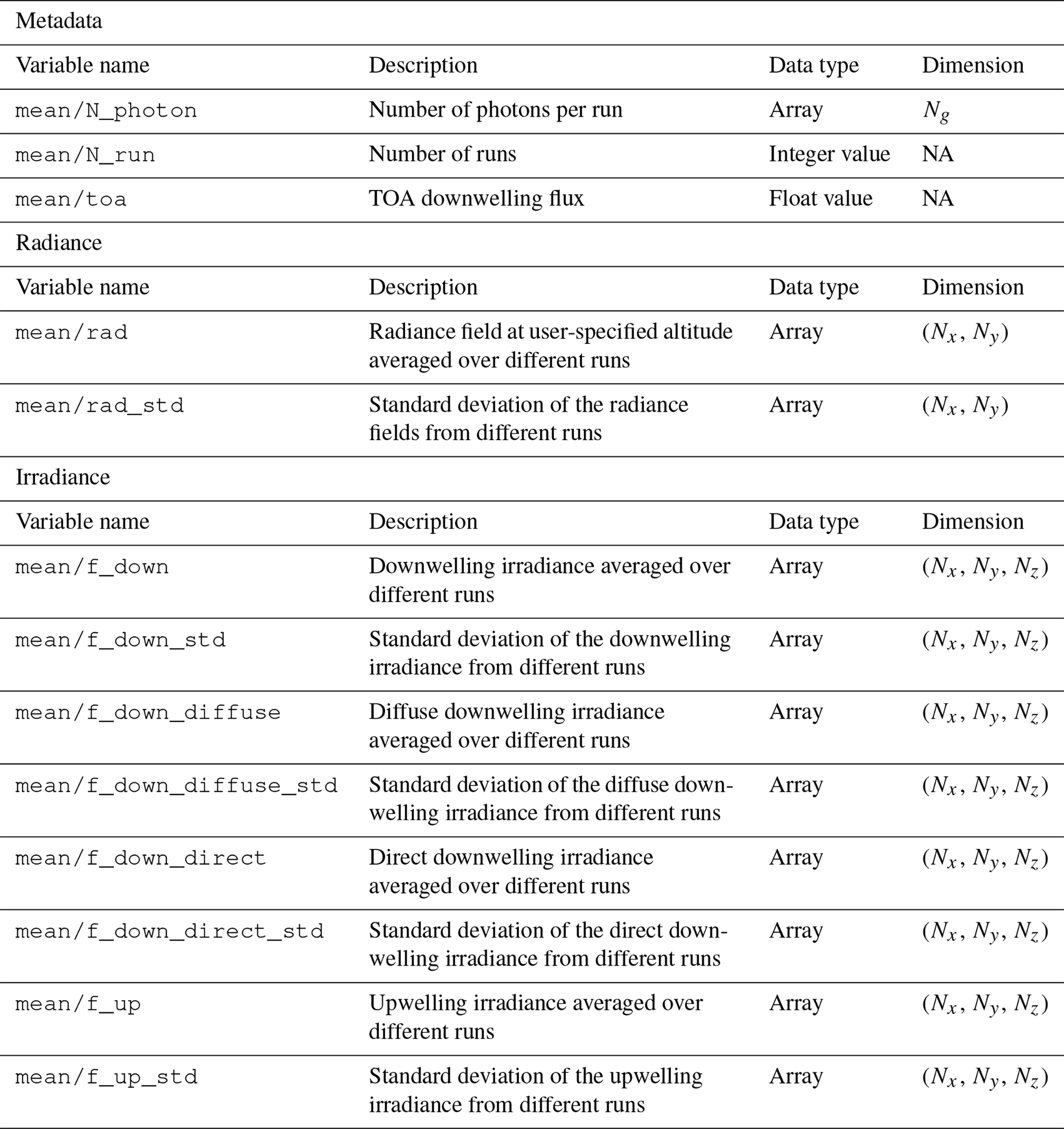
In addition to the example code, intuitive and simple examples are provided in examples/00_er3t_mca.py and examples/00_er3t_lrt.py for users that are interested in learning the basics of setting up EaR³T for calculations. At the current stage, only limited documentation is provided. However, community support is available from the author of this paper through Discord (https://discord.gg/ntqsguwaWv, last access: 6 April 2023). In the near future, more effort will be invested into documentation to give the user more autonomy in creating new applications that cannot be derived from those provided in our paper.

A2 EaR³T code walk-through

We will provide a code walk-through of the OCO-2 and MODIS simulator applications with the code examples/01_oco2_rad-sim.py (App. 1) and examples/02_modis_rad-sim.py (App. 2). The data acquisition (first step in Fig. 1) uses functions in er3t/util. App. 1 and App. 2 use the functions in er3t/util/modis.py and er3t/util/oco2.py for downloading the MODIS and OCO-2 data files from the respective NASA data archives and for processing the data (e.g., geo-mapping, gridding). The user supplies minimum input data (date and time, latitudes and longitudes of the region of interest), which need to be specified in satellite_download (within the application codes). For example, for App. 1 and App. 2, the only user inputs are the date and time and the region of interest (in this case 2 September of 2019, with the westernmost, easternmost, southernmost, and northernmost longitudes and latitudes being 109^∘ W, 107^∘ W, 37^∘ N, and 39^∘ N, respectively). In order for EaR³T to access any data archives, such as NASA Earthdata, the user needs to create an account with them and store the credentials locally (detailed instructions are provided separately along with the EaR³T distribution).

After the data acquisition step, the satellite data are fed into the pre-processing step for (1) atmospheric gases (er3t/pre/atm), (2) clouds (er3t/pre/cld), and (3) surface data (er3t/pre/sfc), as shown in Fig. 1. In the default configuration of the App. 1, the standard US atmosphere (Anderson et al., 1986; included in the EaR³T repository) is used within atm.; EaR³T supports the input of user-specified atmospheric profiles, e.g., atmospheric profiles from reanalysis data for App. 2, by making changes in atm_atmmod (from er3t/pre/atm). Subsequently, molecular scattering coefficients are calculated by cal_mol_ext (from er3t/util), and absorption coefficients for atmospheric gases are generated by (er3t/pre/abs). At the current development stage, the following two options are available:

1. Line-by-line (used by App. 1). The repository includes a sample file of absorption coefficient profiles for a subset of wavelengths within OCO-2's oxygen A-band channel, corresponding to a range of atmospheric transmittance values from low (opaque) to high (so-called “continuum” wavelength). They were generated by an external code based on OCO-2's line-by-line absorption coefficient database (ABSCO; Payne et al., 2020). They are calculated for a fixed mixing ratio of 400 ppm. In a subsequent paper, an OCO-2-specific EaR³T code will be published where the actual mixing ratio is used. For each OCO-2 spectrometer wavelength within a given channel, hundreds of individual absorption coefficient profiles at the native resolution of ABSCO need to be considered across the instrument line shape (ILS, also known as the slit function) of the spectrometer. The ILS, as well as the incident solar irradiance, is also included in the file. In subsequent steps, EaR³T performs RT calculations at the native spectral resolution of ABSCO, but it then combines the output by convolving with the ILS and outputs OCO-2 radiances or reflectances at the subset of wavelengths. For probabilistic (Monte Carlo) RT solvers such as MCARaTS, the number of photons can be kept relatively low (e.g., 10⁶ photons) and can be adjusted according to the values of the ILS at a particular ABSCO wavelength. Any uncertainty at the ABSCO spectral resolution due to photon noise is greatly reduced by convolving with the ILS for the final output.

2. Correlated-k (used by App. 2). This approach (Mlawer et al., 1997) is appropriate for instruments such as MODIS with much coarser spectral resolution than OCO-2 and for broadband calculations. In contrast to the line-by-line approach, RT calculations are not performed at the native resolution of the absorption database but at Gaussian quadrature points (called “g”) that represent the full range of sorted absorption coefficients and then combined using Gaussian quadrature weights. The repository includes an absorption database from Coddington et al. (2008), developed specifically for a radiometer with moderate spectral resolution on the basis of HITRAN (high-resolution transmission molecular absorption database) 2004 (Rothman et al., 2005). It was created for the ILS of the airborne Solar Spectral Flux Radiometer (SSFR, Pilewskie et al., 2003) but is applied to MODIS here, which has a moderate spectral resolution of 8–12 nm with 20–50 nm bandwidth. It uses 16 absorption coefficient bins (g) per target wavelength (this could either be an individual SSFR or a MODIS channel), which are calculated by EaR³T with the Coddington et al. (2008) database using the mixing ratios of atmospheric gases in the previously ingested profile. In future implementations, the code will be updated to enable flexible ILS and broadband calculations.

The er3t/pre/cld module calculates extinction, thermodynamic phase, and effective droplet radius of clouds from the input data. The er3t/pre/pha module creates the required single-scattering albedo and scattering phase function. The default is a Henyey–Greenstein phase function with a fixed asymmetry parameter of 0.85. Along with the current distribution (v0.1.1) of EaR³T, the Mie scattering phase functions based on thermodynamic phase, effective droplet radius, and wavelength are supported. In this study, App. 1 and App. 2 use Mie scattering phase functions calculated from Legendre polynomial coefficients (originally distributed along with libRadtran) based on the wavelength and cloud droplet effective radius. In the future, EaR³T will include standalone phase functions, which can be chosen on the basis of droplet size distributions in addition to effective radius. It is also possible to include aerosols in a similar fashion to how clouds are included. This is done with the er3t/pre/aer module. In the case of aerosols, spectral single-scattering albedo and the asymmetry parameter are required as inputs in addition to the extinction fields.

After the optical properties are calculated, they are passed into the 3D-RT step (er3t/rtm/mca). This step performs the setup of RT solver-specified input parameters and data files, distributing runs over multiple CPUs and post-processing RT output files into a single user-friendly HDF5 file. For example, when radiance is specified as output (default in App. 1 and App. 2), key information such as the radiance field and its standard deviation are stored in the final HDF5 file (for details, see Table 1).

While the EaR³T repository comes with the various applications described above, such as App. 1 and App. 2, the functions used by these master or “wrapper” programs can be organized in different ways, where the existing applications serve as templates for a quick start when developing new applications. The functions used by the master code pass information through the various steps as Python objects. For example, in examples/01_oco2_rad-sim.py, the downloaded and processed satellite data are stored into the sat object. Later, the sat object is passed into an EaR³T function to create the cld object that contains cloud optical properties. Similarly, EaR³T provides functions to create the atm and sfc objects with optical properties for atmospheric gases and the surface. These objects (atm, cld, sfc) are in turn passed on to solver-specific modules for performing RT calculations. The user can choose to save the data of the intermediate objects into Python pickle files after the first run. In this way, multiple calls with identical inputs can reuse existing data, which accelerates the processing time of EaR³T. Unless the user specifies the overwrite keyword argument in the object call to reject saving pickle files, these shortcuts save significant time.

Appendix B: App. 5 radiance calculations based on the large eddy simulation

The CNN COT retrieval framework was developed by Nataraja et al. (2022). It adapts a U-Net (Ronneberger et al., 2015) architecture and treats the retrieval of COT from radiance as a segmentation problem. Probabilities of 36 COT classes (ranging from COT of 0 to 100) are returned as the final COT retrieved for a given cloud radiance field. This method accounts for horizontal photon transport, which is neglected in traditional cloud retrieval algorithms; in other words, for the spatial context of cloudy pixels. It was trained on synthetic cloud fields generated by a large eddy simulation (LES) model, which provides the ground truth of COT. Subsequently, EaR³T was used to calculate 3D-RT radiances at 600 nm for LES cloud fields to establish a mapping between radiance to COT. Only six LES cases were used to represent the variability of the cloud morphology. Each of these fields are 480 × 480 pixels across (spatial resolution of 100 m). These large fields were mapped onto thousands of 64 × 64 mini tiles with spatial resolution of 100 m, as described in Nataraja et al. (2022). To keep the training data set small, mini tiles were selectively sampled according to their mean COT and standard deviation. This ensured an even representation of the dynamic range of COT and its variability, which was termed homogenization of the training data set. Figure B1 shows a collection of samples from the training data as an illustration. All the aforementioned simulation setup and techniques in data process are included in the App. 5 example code, which can be applied to the LES data (a different scene from the six scenes) distributed along with EaR³T.

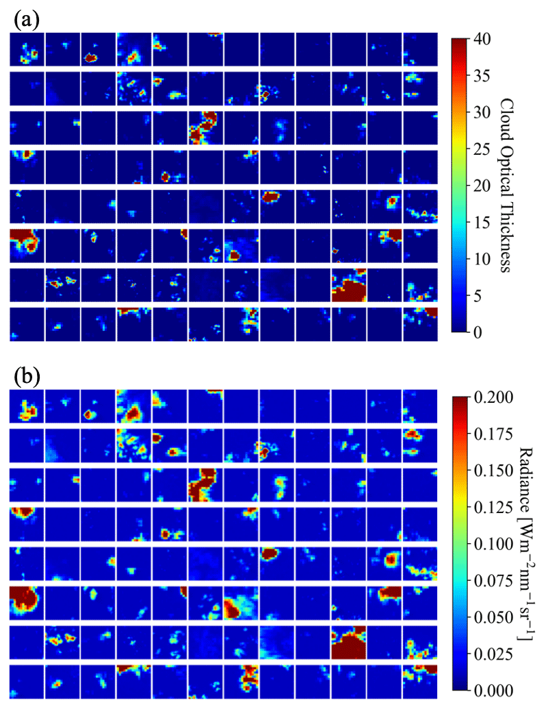
Figure B1 Illustrations of 64 × 64 tiles of (a) cloud optical thickness from LES data and (b) calculated 3D radiance at 600 nm from EaR³T for CNN training.

Appendix C

C1 Cloud detection and identification

Cloudy pixels are identified through a thresholding method based on the red, green, and blue channels of MODIS. When the radiance values of the red, green, and blue channels of a pixel are all greater than a pre-calculated threshold value, the pixel is considered cloudy, as illustrated by the following equation:

$$\begin{array}{}\text{(C1)}& \mathrm{If}\begin{array}{l}\mathrm{Red}>a_{\mathrm{R}}\cdot \mathrm{Quantile}\left(\mathrm{Red},q_{\mathrm{0}}\right)\mathit{\&}\\ \mathrm{Blue}>a_{\mathrm{B}}\cdot \mathrm{Quantile}\left(\mathrm{Blue},q_{\mathrm{0}}\right)\mathit{\&}\\ \mathrm{Green}>a_{\mathrm{G}}\cdot \mathrm{Quantile}\left(\mathrm{Green},q_{\mathrm{0}}\right)\end{array}\left\{\begin{array}{l}\mathrm{Yes}:\mathrm{cloudy}\\ \mathrm{No}:\mathrm{clear}\mathrm{sky}\end{array}\right.,\end{array}$$

where a_R, a_B, and a_G are scale factors with a default value of 1.0, and quantile returns the q₀ percentile of the sorted reflectance data (in ascending order; q₀=0.5 is equivalent to the median). The scale factors can be adjusted separately to perform fine tuning for different surface types. For example, adjusting a_G will be more effective for separating clouds from greenish vegetation surface than the other two factors. For simplicity, they are all set to 1.0 for the case shown in App. 1 and 2. The q₀ is determined by the following equation:

$$\begin{array}{}\text{(C2)}& q_{\mathrm{0}}=max(\mathrm{0},\mathrm{1}-{\mathrm{frac}}_{\mathrm{cld}}\cdot \mathrm{1.2}),\end{array}$$

where frac_cld is cloud fraction obtained from the MODIS L2 cloud product (number of cloudy pixels divided by the number of total pixels). Through the definition of q₀, the threshold-based cloud detection method is pegged to the MODIS product at the domain scale. Because of the coarse resolution of the MODIS-based cloud mask, it cannot be used directly for our application. However, it uses many more channels than available at high spatial resolution and is therefore more accurate. The factor of 1.2 can be adjusted. A value of higher than 1 allows for clouds that are not detected by MODIS (for various reasons, for example because of their spatial scale) to be picked up. At the same time, this leads to over-detection (false positives, i.e., clear-sky pixels identified as cloudy), and therefore the thresholding is only the first step (primary thresholding), followed by the next (secondary) step where false positives are removed.

The secondary step is based on MODIS L2 cloud products: COT (cloud optical thickness), CER (cloud effective radius), and CTH (cloud top height). For the pixels that are identified as cloudy in the primary thresholding, especially at the lower end of the reflectance (Ref.), we rely on the clear-sky identifiers from MODIS L2 cloud product (where no cloud products are retrieved), as illustrated by the following equation

$$\begin{array}{}\text{(C3)}& \mathrm{If}\begin{array}{l}\mathrm{Ref}.<\mathrm{Median}\left(\mathrm{Ref}.\right)\mathit{\&}\\ \mathrm{COT},\mathrm{CER},\mathrm{and}\mathrm{CTH}\mathrm{are}\mathrm{NaN}\end{array}\left\{\begin{array}{l}\mathrm{Yes}:\mathrm{clear}\mathrm{sky}\\ \mathrm{No}:\mathrm{cloudy}\end{array}\right..\end{array}$$

Figure C1 shows the cloud mask from primary thresholding (Eq. C1, red and purple) and the pixels that are reverted to clear sky by the secondary filter (Eq. C2, red).

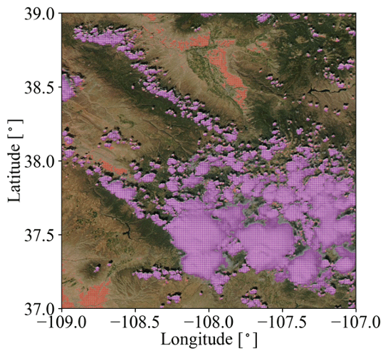
Figure C1 Cloud mask for the scene shown in Fig. 2. Red and purple indicate the pixels identified as cloudy through the primary thresholding (Eq. C1), and purple indicates the pixels identified as cloudy after applying the secondary filter (Eq. C3).

C2 IPA reflectance-to-COT mapping

In order to retrieve COT (cloud optical thickness) from cloud reflectance as measured by various instruments, we use the EaR³T built-in solver MCARaTS in IPA mode to calculate a lookup table of reflectance as a function of COT. The function for generating these lookup tables is included in EaR³T as er3t.rtm.mca.func_ref_vs_cot. Two mappings are generated for Apps. 1 and 2 to account for geometrically thin (cloud top height less than 4 km) and thick (cloud top height greater than 4 km) clouds separately, while a single mapping is generated for App. 4. Specifically, for a range of COT (0 to 200), reflectance is calculated from EaR³T with the same input parameters (wavelength, viewing and solar geometries, and surface albedo) listed in Table A1 for each application except for a few simplifications described in Table C1.

Table C1 List of parameters for deriving IPA reflectance-to-COT (cloud optical thickness) mappings for Apps. 1 and 2 and App. 4 in addition to those listed in Table A1.

The clouds are assumed to be horizontally homogeneous over a 2×2 pixel domain. For each calculation, 10⁸ photons are used for running EaR³T in IPA mode. After calculating R(COT), the inverse relationship of COT(R) is then used for estimating COT at any given R for the cloudy pixels. Figure C2 shows the IPA reflectance-to-COT mappings created for Apps. 1 and 2 and App. 4. Note that the difference between the Apps. 1 and 2 thin clouds (blue) and App. 4 (green) is due to different surface albedos (when COT is less than 20) and sensor-viewing geometries (when COT greater than 20, specified in Table A1). Note that this approach will ensure IPA radiance and reflectance consistency (retrieved IPA COT will reproduce the exact IPA cloud reflectance; see Fig. C3) because the radiative transfer processes of R(COT) and COT(R) are the same. However, since it makes some simplifications, as mentioned above, uncertainties are expected for a complicated atmospheric environment (varying cloud thermodynamic phase, effective radius, cloud top height, geometrical thickness, and vertical profile and variable surface albedo and topography), which show up as spread (deviations from identity line) in Fig. C3.

Figure C2 The IPA reflectance-to-COT mappings used for Apps. 1 and 2 (red and blue) and App. 4 (green). The reflectance is normalized by the cosine of solar zenith angle (referred to as solar noon reflectance). The uncertainties associated with photon statistics are indicated by the shaded area.

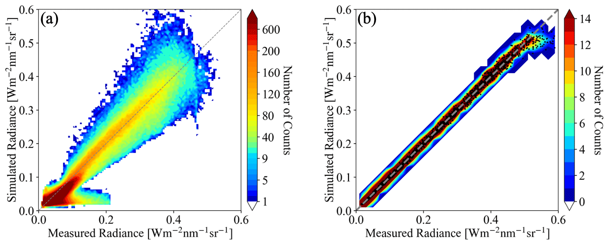
Figure C3 Panels (a) and (b) are the same as Figs. 7 and 13b except for the IPA radiance calculations.

Appendix D

D1 Parallax correction

From the satellite's view, the clouds (especially high clouds) will be placed at inaccurate locations on the surface, which have shifted from their actual locations due to the parallax effect. We followed simple trigonometry to correct for it as follows.

Longitude correction (positive from west to east) is performed using the following equation:

$$\begin{array}{}\text{(D1)}& \mathit{\delta }\mathrm{long}={\displaystyle \frac{\left(z_{\mathrm{cld}}-z_{\mathrm{sfc}}\right)\cdot \tan \left(\mathit{\theta }\right)\cdot \sin \left(\mathit{\varphi }\right)}{\mathit{\pi }\cdot R_{\mathrm{Earth}}}}\times \mathrm{180}{}^{\circ },\end{array}$$

and latitude correction (positive from south to north) is performed using the following equation:

$$\begin{array}{}\text{(D2)}& \mathit{\delta }\mathrm{lat}={\displaystyle \frac{\left(z_{\mathrm{cld}}-z_{\mathrm{sfc}}\right)\cdot \tan \left(\mathit{\theta }\right)\cdot \cos \left(\mathit{\varphi }\right)}{\mathit{\pi }\cdot R_{\mathrm{Earth}}}}\times \mathrm{180}{}^{\circ },\end{array}$$

where (long_sat, lat_sat, z_sat) is the satellite location and θ and ϕ (0^∘ at north, positive clockwise) are the sensor-viewing zenith and azimuth angles. z_cld and z_sfc are the cloud top height and the surface height. R_Earth is the radius of the Earth. Figure D1 shows an illustration of the parallax correction for the cloud field in the inset in Fig. 2. Note that discontinuities in the latitude and longitude fields arising from different combinations of sensor-viewing geometries and cloud top and surface heights may lead to gaps in the cloud fields. These gaps are identified and filled in with the average of data from adjacent pixels (plus or minus two pixels along x and y) through the following process:

$$\begin{array}{}\text{(D3)}& \begin{array}{rl}& \mathrm{If}\begin{array}{l}{\mathrm{pixel}}_{ij}^{\mathrm{aft}}\mathrm{is}\mathrm{clear}\mathrm{\&}{\mathrm{pixel}}_{ij}^{\mathrm{bef}}\mathrm{is}\mathrm{cloudy}\mathit{\&}\\ \mathrm{cldfrac}\left({\mathrm{pixel}}^{\mathrm{bef}}\left[i-\mathrm{2}:i+\mathrm{2},j-\mathrm{2}:j+\mathrm{2}\right]\right)>{\mathrm{frac}}_{\mathrm{a}}\mathit{\&}\\ \mathrm{cldfrac}\left({\mathrm{pixel}}^{\mathrm{aft}}\left[i-\mathrm{2}:i+\mathrm{2},j-\mathrm{2}:j+\mathrm{2}\right]\right)>{\mathrm{frac}}_{\mathrm{b}}\mathit{\&}\end{array}\\ & \left\{\begin{array}{l}\mathrm{Yes}:\mathrm{fill}{\mathrm{pixel}}_{ij}^{\mathrm{aft}}\mathrm{with}\mathrm{the}\mathrm{average}\mathrm{of}\\ \mathrm{cld}\left({\mathrm{pixel}}^{\mathrm{aft}}\left[i-\mathrm{2}:i+\mathrm{2},j-\mathrm{2}:j+\mathrm{2}\right]\right)\end{array}\right.,\end{array}\end{array}$$

where pixel_ij indicates the pixel at i along x and j along y; bef and aft refer to before and after parallax correction, respectively; cldfrac calculates cloud fraction (number of cloudy pixels divided by total pixel number); and cld selects data where pixels are identified as cloudy. The frac_a and frac_b are set to 0.7 for the cases demonstrated in the paper. Lower frac_a tends to over-select clear-sky pixels at the cloud edge, and lower frac_b tends to overcorrect clear-sky pixels within clouds that are not clear-sky pixels due to parallax artifacts. Increasing frac_a and frac_b values tends to under-correct parallax artifacts.

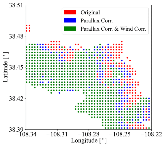
Figure D1 An illustration of correcting cloud location (red) for parallax effect (blue) and wind effect (green) for the cloud field of the inset in Fig. 2. Filled cloud gaps are as described in Appendix D1 are indicated by black circles.

D2 Wind correction

The wind correction aims to correct the movement of clouds when advected by the wind between two different satellite overpasses.

Longitude correction (positive from west to east) is performed using the following equation:

$$\begin{array}{}\text{(D4)}& \mathit{\delta }\mathrm{long}={\displaystyle \frac{\stackrel{\mathrm{‾}}{u}\cdot \mathit{\delta }t}{\mathit{\pi }\cdot R_{\mathrm{Earth}}}}\times \mathrm{180}{}^{\circ },\end{array}$$

and latitude correction (positive from south to north) is performed using the following equation:

$$\begin{array}{}\text{(D5)}& \mathit{\delta }\mathrm{lat}={\displaystyle \frac{\stackrel{\mathrm{‾}}{v}\cdot \mathit{\delta }t}{\mathit{\pi }\cdot R_{\mathrm{Earth}}}}\times \mathrm{180}{}^{\circ },\end{array}$$

where $\stackrel{\mathrm{‾}}{u}$ and $\stackrel{\mathrm{‾}}{v}$ are the domain-averaged 10 m zonal and meridional wind speeds and δt is the time difference between two different satellites that fly on the same orbit. Figure D1 shows the cloud location after applying the parallax (Appendix D1) and wind correction for the cloud field in the inset from Fig. 2.