Stratospheric temperature measurements from nanosatellite stellar occultation observations of refractive bending

Stellar occultation observations from space can probe the stratosphere and mesosphere at a fine vertical scale around the globe. Unlike other measurement techniques like radiosondes and aircraft, stellar occultation has the potential to observe the atmosphere above 30 km, and unlike radio occultation, stellar occultation probes fine-scale phenomena with potential to observe atmospheric turbulence. We imaged the refractive bending angle of a star centroid for a series of occultations by the atmosphere. Atmospheric refractivity, density, and then temperature are retrieved from the bending observations with the Abel transformation and Edlén's law, the hydrostatic equation, and the ideal gas law. The retrieval technique is applied to data collected by two nanosatellites operated by Terran Orbital. Measurements were primarily taken by the GEOStare SV2 mission, with a dedicated imaging telescope, supplemented with images captured by spacecraft bus sensors, namely the star trackers on other Terran Orbital missions. The bending angle noise floor is 10 and 30 arcsec for the star tracker and GEOStare SV2 data, respectively. The most significant sources of uncertainty are due to centroiding errors due to the fairly low-resolution stellar images and telescope pointing knowledge derived from noisy satellite attitude sensors. The former mainly affects the star tracker data, while the latter limits the GEOStare SV2 accuracy, with both providing low vertical resolution. This translates to a temperature profile retrieval up to roughly 20 km for both star tracker and GEOStare SV2 datasets. In preparation of an upcoming 2023 mission designed to correct these deficiencies, SOHIP, we simulated bending angle measurements with varying magnitudes of error. The expected maximum altitude of retrieved temperature is 41 km on average for these simulated measurements with a noise floor of 0.39 arcsec. Our work highlights the capabilities of stellar occultation observations from nanosatellites for atmospheric sounding. Future work will investigate high-frequency observations of atmospheric gravity waves and turbulence, mitigating the major uncertainties observed in these datasets.

1 Introduction

Occultation measurement techniques perform atmospheric sounding by observing the perturbation in a signal that passes through the atmosphere. A signal source on the opposite side of the Earth from a satellite is tracked as the line of sight between them passes deeper into the atmosphere until the Earth limb obscures the signal completely. The signals utilized for radio occultation (RO) and stellar occultation (SO) are radio waves from Global Positioning System (GPS) satellites and optical waves from starlight, respectively. SO was first described by Jones et al. (1962), while Yunck et al. (1988) first described RO. Since 1995 many RO missions have retrieved atmospheric density and temperature accurately in the upper troposphere and lower stratosphere up to 30–35 km (Hajj et al., 2002), which are utilized for research on diverse topics like numerical weather prediction and deep convection in the tropics (Anthes, 2011; Scherllin-Pirscher et al., 2021). SO has been utilized to study Earth's atmosphere via refraction (White et al., 1983; Yee et al., 2002; Sofieva et al., 2003). In 2002, the first instrument dedicated to SO was launched on the ENVISAT (ENVIronmental SATellite) platform. The instrumentation utilizes absorptive SO techniques to observe O₃ trends (Bertaux et al., 2010).

Both RO and SO are intrinsically relative measurements since they observe the change in a signal with and without attenuation from the atmosphere to determine atmospheric properties. This feature makes these techniques perfect candidates for long-term observations since there is minimal measurement drift. Additionally, both techniques utilize an already existing signal (starlight and GPS radio waves for SO and RO, respectively) and only require the signal detector or receiver on board the payload. The biggest difference between the two occultation methods is the wavelength of the signal. The small wavelength of optical waves compared to microwaves allows SO to interrogate small spatial scales and observe atmospheric turbulence (Gurvich and Kan, 2003a, b; Sofieva et al., 2007, 2019). This work focuses on refractive SO because of the potential to measure both temperature and turbulence.

Previous SO Earth observations were performed on large satellites: Orbiting Astronomical Observatory (OAO-2), Mir satellite, Global Ozone Monitoring by Occultation of Stars (GOMOS) on ENVISAT, and Ultraviolet and Visible Imagers and Spectrometers (UVISI) on the Midcourse Space Experiment (MSX) (Hays and Roble, 1973; Gurvich and Kan, 2003a; Bertaux et al., 2010; Yee et al., 2002). As noted above, SO only requires a signal detector, which does not require a large or complex platform. Additionally, refractive SO requires high-quality camera optics compared to the spectrometer necessary for absorptive SO, and hence a much smaller platform can be used for refractive SO.

Developments in spacecraft technology since 1997 have spurred exponential growth in launch rates of “nanosatellites” with 1–10 kg mass (Janson, 2020). Nanosatellites are also at least 100 times cheaper and much quicker to launch than typical full-scale satellites (Woellert et al., 2011). We can launch multiple nanosatellites for the same cost of a full-scale satellite and observe the atmosphere with a higher temporal resolution. Alternatively, multiple nanosatellites can perform measurements at various angles, enabling advanced retrieval techniques like tomography. The trade-off for the nanosatellite low cost is a satellite with decreased stability. However, we can mitigate the nanosatellite instability by utilizing two cameras: a wide-view camera to image reference stars and a narrow-view camera to observe occulting stars. This paper describes the refractive SO technique utilized to perform atmospheric sounding in Sect. 2. Then, two datasets from operational nanosatellites are presented and analyzed for a proof of concept in Sect. 3. Sounding observations from a star tracker are presented in Sect. 3.1. Observations from a high-resolution telescope on board the GEOStare SV2 nanosatellite are shown in Sect. 3.2. Section 4 analyzes the retrieval error with varying levels of simulated instrument error and compares the results to the observed error from the star tracker and GEOStare SV2 data. Finally, Sect. 6 discusses the improvements necessary to make the SO technique viable for observing stratospheric properties.

2 Description of the stellar occultation sounding technique

Remote atmospheric sounding with refractive stellar occultation (SO) utilizes images of a star as it sets below the Earth's horizon to determine the atmospheric temperature vertical profile. Section 2.1 describes how the ray “bends” due to the refractive index profile, and Sect. 2.2 describes the method(s) to determine the observed refractive bending angle vertical profile from the satellite images.

The observed bending at each level is due to changes in the refractive index along the line of sight from the satellite to the star, so an observation at a particular altitude is an integrated measurement from the ray perigee to the top of the atmosphere. Thus, the refractive index vertical profile can be retrieved from the observed overall bending angle with an “onion-peeling” inversion approach. Section 2.3 describes the retrieval technique, the equations to determine atmospheric state based on the retrieved refractive index profile, and the effect of instrument error on the retrieved profile. The atmospheric properties determined from these measurements include density, pressure, and temperature.

2.1 Atmospheric refraction forward model

The SO atmospheric sounding technique observes the atmosphere's effect on light generated by a star. The atmosphere appears to “bend” light that passes through due to the atmospheric gradient in refractive index. The atmospheric vertical profile of refractive index n(z) varies with atmospheric density ρ(z) based on the surface density ρ₀ for a wavelength λ (Edlén, 1966):

$$\begin{array}{}\text{(1)}& n\left(z\right)=\mathrm{1}+C\left(\mathit{\lambda }\right){\displaystyle \frac{\mathit{\rho }\left(z\right)}{{\mathit{\rho }}_{\mathrm{0}}}},\end{array}$$

where C(λ) is a dispersion factor describing the variation of refractive index with wavelength (Barrell and Sears, 1939).

$$\begin{array}{}\text{(2)}& C\left(\mathit{\lambda }\right)={\mathrm{10}}^{-\mathrm{8}}\left(\mathrm{8342.13}+{\displaystyle \frac{\mathrm{2.406}\times {\mathrm{10}}^{\mathrm{6}}}{\mathrm{130}-{\mathit{\lambda }}^{-\mathrm{2}}}}+{\displaystyle \frac{\mathrm{15}\mathrm{997}}{\mathrm{38.9}-{\mathit{\lambda }}^{-\mathrm{2}}}}\right)\end{array}$$

The refractive index profile can be written in terms of atmospheric pressure P(z) and temperature T(z) profiles based on the ideal gas law with gravitational acceleration g and the specific gas constant for dry air R_air. Based on the hydrostatic equation and a known temperature gradient $\mathrm{d}T/\mathrm{d}z$, the refractive index vertical gradient is differentiated from Eq. (1):

$$\begin{array}{}\text{(3)}& {\displaystyle \frac{\mathrm{d}n}{\mathrm{d}z}}=-C\left(\mathit{\lambda }\right){\displaystyle \frac{T_{\mathrm{0}}P\left(z\right)}{P_{\mathrm{0}}T(z{)}^{\mathrm{2}}}}\left({\displaystyle \frac{g}{R_{\mathrm{air}}}}+{\displaystyle \frac{\mathrm{d}T}{\mathrm{d}z}}\right).\end{array}$$

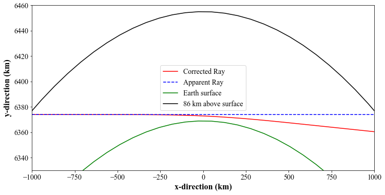
Figure 1 Example of ray trajectory through an atmospheric profile from MERRA2. The black and green lines do not look circular because of the different x and y scales. Ray tracing computes both the ray perigee and the bending angle for an apparent ray. Here, an apparent ray perigee of 5 km results in a corrected ray perigee of 3.77 km with 2914 arcsec bending angle.

The refractive index profile and its gradient are used in the Eikonal equation to model the path of a ray passing through the atmosphere. A ray with position $\mathit{x}=(x,y,z)$ in Cartesian coordinates along its path s is traced with

$$\begin{array}{}\text{(4)}& {\displaystyle \frac{{\mathrm{d}}^{\mathrm{2}}\mathit{x}}{\mathrm{d}{\mathit{\tau }}^{\mathrm{2}}}}=n\mathrm{\nabla }n,\end{array}$$

where $\mathrm{d}\mathit{\tau }=\mathrm{d}s/n$ (Zou et al., 1999). The ray-tracing equation above is integrated in 1D assuming that the atmospheric refractive index vertical profile does not vary with latitude or longitude. Tracing the ray starts at the orbiting satellite telescope located 430 km above the Earth's surface. The ray direction is initialized from the satellite position with a vector pointing toward its apparent ray perigee, i.e., the altitude of the point closest to the surface. Then, the corrected ray path is calculated by integrating the Eikonal equation (Eq. 4) based on a vertical profile of temperature and pressure. The atmospheric profile utilized here is from the Modern-Era Retrospective analysis for Research and Applications Version 2 (MERRA2) reanalysis dataset (GMAO, 2015b). Figure 1 shows that the actual ray path due to refraction results in a corrected ray perigee of 3.77 km for an apparent ray with a line-of-sight perigee of 5 km, and Fig. C1 shows the ray perigee correction for several line-of-sight perigees. The angle between the corrected ray and the line of sight, normal to the Earth's surface, is the refractive bending angle, which is 2900 arcsec in Fig. 1. The top of the atmosphere, above which the refractive bending angle is negligible, is assumed to be 86 km, corresponding to approximately 5 km above the maximum altitude predicted by MERRA2.

2.2 Refractive bending observations

Observing the bending angle is accomplished by commanding a camera to capture images in inertial pointing mode with the telescope pointed at the star of interest. Any motion of the star relative to its initial position is attributed to changes in the refractive index of the atmosphere, and we track the star position to calculate the vertical profile of observed refractive bending angles. First, we determine the star centroid position on each image in terms of pixels on the field of view during an occultation session. Next, we find the location of the field of view in the sky using stars above the atmosphere, so the star position on each image can be compared on an absolute reference frame. The bending angle of the star of interest in each image is determined from the star's centroid change in position on the absolute reference frame, and we calculate the apparent and corrected ray perigees.

2.2.1 Centroid position

Diffraction of a stellar point source in the telescope is captured on the detector as a point spread function (PSF). Irregular deviations in the optical surfaces and atmospheric seeing conditions may result in a Moffat PSF (Moffat, 1969). In this work, we find the centroid location on the image (x₀,y₀) by solving a nonlinear least-square problem fitting a PSF to the observed star centroid within a square region of 20 by 20 pixels. The two functions we used are the 2D Gaussian (f_g) and Moffat (f_m) distributions.

$$\begin{array}{}\text{(5)}& {\displaystyle }{f}_{\mathrm{g}}(x,y)=A_{\mathrm{g}}\exp \left\{-{\displaystyle \frac{(x-x_{\mathrm{0}}{)}^{\mathrm{2}}}{{\mathit{\sigma }}_x^{\mathrm{2}}}}-{\displaystyle \frac{(y-y_{\mathrm{0}}{)}^{\mathrm{2}}}{{\mathit{\sigma }}_y^{\mathrm{2}}}}\right\}\text{(6)}& {\displaystyle }{f}_{\mathrm{m}}(x,y)=A_{\mathrm{m}}{\left(\mathrm{1}+{\displaystyle \frac{(x-x_{\mathrm{0}}{)}^{\mathrm{2}}+(y-y_{\mathrm{0}}{)}^{\mathrm{2}}}{B^{\mathrm{2}}}}\right)}^{-\mathit{\beta }}\end{array}$$

Both PSFs require three parameters in addition to the centroid location: a parameter for the peak intensity (A_g or A_m) and two parameters describing the distribution shape. The 2D Gaussian includes σ_x and σ_y for the x and y width in pixels, respectively. The Moffat distribution includes a width parameter B and a negative exponent, −β, that determine the PSF shape. The Moffat distribution is similar in shape to a Gaussian with a tail or “wing” that becomes more prominent as β decreases with typical values below 5 (Trujillo et al., 2001). The centroid data fit to a Moffat PSF in this work (see Sect. 3.1) results in widths of 0.43 to 2.5 pixels (approximately 13 to 77 arcsec) and β values from 0.8 to 1.18.

2.2.2 Bending angle

In inertial pointing mode, the camera keeps pointing at the same star field as the payload orbits. However, spacecraft pointing is not perfectly steady due to drift and jitter, and this motion must be accounted for to determine the relative change in the centroid as the starlight passes deeper into the atmosphere. The camera view is defined by its boresight, or center of the image specified by its coordinates in right ascension (RA) and declination (DEC), along with camera rotation around the boresight. These parameters can be calculated at the time of exposure by finding an astrometric solution for the star field above the atmosphere, or they can be estimated from the payload attitude and position control system. The World Coordinate System (WCS) defined by these parameters is utilized to translate the centroid location on each image to a stabilized reference frame.

The stabilized reference frame is chosen as the average WCS among all images with boresight ray perigees above 100 km. The actual coordinate of the star is determined by the average world coordinate (RA^∗, DEC^∗) among all images with boresight ray perigees above 100 km. The refractive bending angle of each image is determined by calculating the Euclidean distance from the reference coordinate's pixel location on the image to the observed centroid pixel location. The detector plate scale (pixels per radian) is used to convert the pixel distance to the refractive bending angle.

2.2.3 Ray perigee

The apparent and corrected ray perigees must be calculated for each image based on the information known about the telescope's pointing and the observed star position since the star is not necessarily in the center of the image. We utilize two approaches to determine the apparent ray perigee of each measurement with the Ansys Systems Tool Kit (STK) depending on the data available. STK is software that simulates platforms and payloads including satellites based on the known satellite location and orbit. As explained next, we use a direct approach if accurate information for the camera WCS is available at each exposure time. Otherwise a rotated approach is used.

Direct. The direct approach utilizes the STK software to draw a vector directly from the satellite position to the observed centroid coordinate. The coordinate is determined from the image WCS and the centroid location on the image. The software determines the point along the vector closest to the Earth's surface and returns the altitude, latitude, and longitude of the ray perigee. This method is best suited for scenarios with high certainty in the image WCS since it defines the line-of-sight vector.

Rotated. The rotated approach utilizes the star reference coordinate and bending angle instead of the image WCS. Although the WCS is used in calculating the bending angle as described above, it is not directly used by STK so that the ray perigee is less sensitive to errors in the image WCS. Here, a reference vector is drawn from the satellite to the occulted star's actual coordinate. This vector is rotated normal to the Earth's surface by the observed refractive bending angle. Then, the ray perigee and its latitude and longitude are accessed from the rotated vector's point closest to the Earth's surface.

2.3 Retrieval technique

The observations result in a vertical profile of refractive bending angle. To investigate the underlying atmospheric state, these observations must be inverted for the refractive index vertical profile. Then, the inverse of Eq. (1) is applied to estimate atmospheric density.

2.3.1 Bending angle inversion

The refractive index profile can be retrieved by applying the inverse Abel transform to the bending angles α observed above a particular ray perigee (z) (Sofieva and Kyrölä, 2004). The Abel integral is relative to an impact parameter p=n(z)r, where r is the distance from the Earth's center, $r=z+r_{\mathrm{E}}$, assuming the Earth's radius r_E=6371 km. However, since the atmospheric refractive index, n(z), is between 1 and 1.0001 at altitudes above 10 km, n can be neglected so that $p\approx z+r_{\mathrm{E}}$. Applying the Abel inversion to the bending angle profile estimates the refractive index as a function of r:

$$\begin{array}{}\text{(7)}& \ln \left(n\right(r\left)\right)={\displaystyle \frac{\mathrm{1}}{\mathit{\pi }}}\underset{r}{\overset{\mathrm{\infty }}{\int }}{\displaystyle \frac{\mathit{\alpha }\left(a\right)}{\sqrt{a^{\mathrm{2}}-r^{\mathrm{2}}}}}\mathrm{d}a,\end{array}$$

where a corresponds to the distance from Earth's center. The inversion algorithm is adapted from the Radio Occultation Processing Package (Culverwell et al., 2015).

2.3.2 Temperature calculation

Since atmospheric density is related to the refractive index, as described in Eq. (1), we estimate the atmospheric density profile from the retrieved refractive index profile based on Edlén's equation with C(λ) described by Eq. (2).

$$\begin{array}{}\text{(8)}& \mathit{\rho }\left(z\right)={\displaystyle \frac{n\left(z\right)-\mathrm{1}}{C\left(\mathit{\lambda }\right)}}{\mathit{\rho }}_{\mathrm{0}}\end{array}$$

The hydrostatic equation relates atmospheric pressure and density profiles so the pressure vertical profile can be estimated from the atmospheric density profile with Eq. (9). Then, the ideal gas law determines atmospheric temperature based on the pressure and density, so the temperature vertical profile is estimated from the retrieved refractive index using Eq. (10).

$$\begin{array}{}\text{(9)}& {\displaystyle }P\left(h\right)=\underset{h}{\overset{\mathrm{\infty }}{\int }}\mathit{\rho }\left(z\right){\displaystyle \frac{g{r}_{\mathrm{E}}^{\mathrm{2}}}{(r_{\mathrm{E}}+z{)}^{\mathrm{2}}}}\mathrm{d}z\text{(10)}& {\displaystyle }T\left(h\right)={\displaystyle \frac{P\left(h\right)}{R_{\mathrm{air}}\mathit{\rho }\left(h\right)}}\end{array}$$

3 Satellite measurements

Refractive stellar occultation measurements were collected with two different nanosatellite instruments in orbit. Both satellites were launched and operated by Terran Orbital. Observations collected by a star tracker on board a nanosatellite between September and October 2020 are referred to as ST data. Observations tasked by Lawrence Livermore National Laboratory with operation by Terran Orbital between November 2021 and April 2022 with a similar nanosatellite and high-resolution telescope are referred to as GEOStare SV2 data (GEOsynchronous Space Telescopes for Actionable Refinement of Ephemeris Space Vehicle 2 – see Simms et al., 2013). Figure 2 shows an image of the same star field captured by the telescopes for ST and GEOStare SV2. The smaller GEOStare SV2 field of view is roughly drawn onto the star tracker image in Fig. 2a to show their respective fields of view (FOVs).

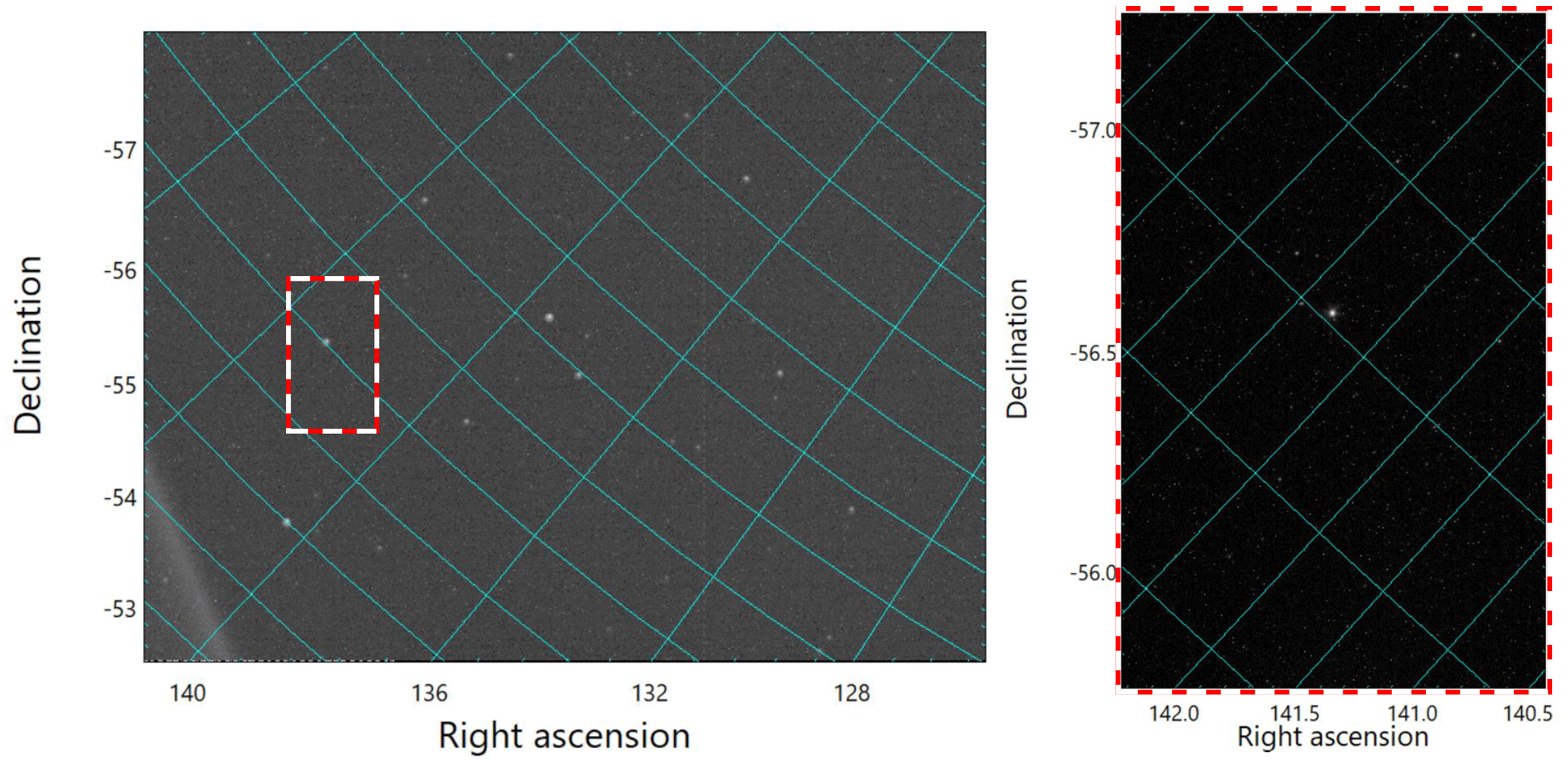
Figure 2 A star field imaged by both the star tracker and GEOStare SV2. The ST image shows the GS2 field of view approximately drawn as a dashed red and white rectangle.

ST utilizes a telescope with 14 mm aperture diameter and a 10.7^∘ × 7.8^∘ field of view. The sensor is a MT9M021 CMOS from ON Semiconductor with a 3.75 µm pixel size for a plate scale of 30.9 arcsec per pixel operated at a frame rate of 0.5 Hz.

GEOStare SV2 utilizes a telescope with 85 mm aperture diameter and field of view of 2.12^∘ × 1.33^∘. The sensor is a ASI174MM camera from ZWO with a 5.86 µm pixel size for a plate scale of 4 arcsec per pixel operated at a frame rate of 1 Hz.

Figure 2a and b show the same star field captured by ST and GEOStare SV2 with exposure times of 0.284 and 0.5 s, respectively. The spatial resolution with GEOStare SV2 is much higher than the ST, as shown by the significantly smaller field of view projected to the ST view outlined in red and white dashes in Fig. 2a. The telescope utilized by the GEOStare SV2 mission was designed by Bauman and Pertica (2021) and Riot et al. (2017). GEOStare SV2 was designed for space situational awareness applications, while the ST instrument is intended to be a compact, inexpensive, high-accuracy star tracker. Neither payload was specifically designed for stellar occultation, but they were operated to acquire proof-of-concept data to assess our sounding technique before an instrument designed for stellar occultation is launched.

3.1 Star tracker observations

Although the ST instrument profiles the atmosphere at a low frequency of 0.5 Hz and captures low-resolution star field images at 30.7 arcsec per pixel, the large field of view and long exposure time (0.24–0.55 s) allow an accurate estimate of the telescope boresight or WCS, consistent with its intended application as a star tracker. These observations targeted stars with apparent magnitude 2.35–2.54, so each image captured several stars that were unaffected by the atmosphere or planet in addition to the targeted star. These factors allowed the calculation of an astrometric solution with an uncertainty of 0.3 arcsec.

We collected data from 217 sessions, with each session including between 15 and 40 images that captured the transit of stars behind the atmosphere with up to 70 unique stars per session. Not all stars captured are good candidates for stellar occultation since the star needs to be bright, but not so bright that it saturates the camera. In addition, not all stars are occulted by the atmosphere during a session. After analyzing the data, we chose the 10 brightest occultation events that were not saturated to analyze. We found that the vertical resolution ranges from 3 to 8 km among these 10 occultation events.

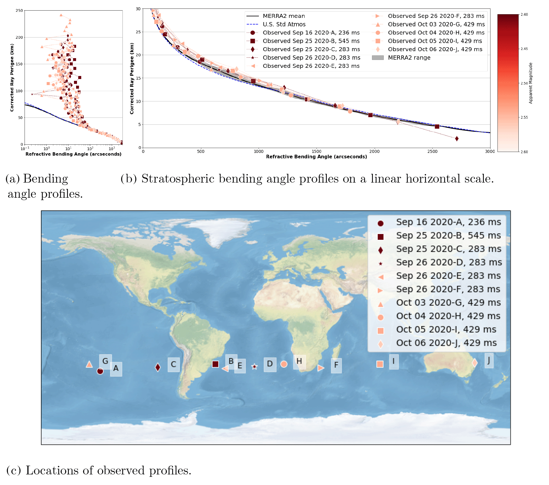
Figure 3 ST observations compared to MERRA2 and US Standard Atmosphere in panels (a) and (b) and their locations in panel (c). The gray region is the range of bending angles from MERRA2 across all of our observations. The color of each observation dataset corresponds to the color bar showing apparent magnitude of the star captured from dimmest (2.6) to brightest (2.4). Panel (a) shows the full atmospheric sounding on a logarithmic scale, and (b) shows the profile in the stratosphere on a linear scale. The exposure time of each session's images is listed in the legend entry.

Figure 3 shows the ST observations and their locations within the southern subtropics between 26 and 34^∘ S. The observations were not aimed at a particular geographic location, so the combination of the camera operation limiting the brightness of stars, filtering data for the brightest stars, and orientation of the star tracker camera led to unintentionally targeting the southern subtropics. Figure 3a and b show the full profile and a zoomed in profile of the stratosphere, respectively, with the observed refractive bending angle in diamond markers from 10 sessions. Figure 3b also shows model predictions of the bending angle by applying the ray-tracing model to the 1976 US Standard Atmosphere (NOAA NASA US Air Force, 1976) as the dashed blue line. The MERRA2 model-predicted temperature and density profiles from the GMAO (2015a, b) for each occultation session's date and location are used to calculate an estimate of the bending angle, which is shown with the average profile as the black line, and the range among the different times and locations is in the gray shaded region.

The observed bending angle is calculated from the captured images using the Moffat PSF described in Sect. 2.2.1 to determine the centroid locations, and the ray perigee is determined with the direct method described in Sect. 2.2.3.

The bending angle observations correlate slightly better with the MERRA2 reanalysis data than the US Standard Atmosphere, with correlation coefficients of 0.986 and 0.983, respectively. The parity plot is shown in the Appendix in Fig. C2. The MERRA2 model is much more accurate since it is a global reanalysis model actively developed, so observations correlating with MERRA2 better than the US Standard Atmosphere provides confidence in these measurements.

3.2 GEOStare SV2 observations

We scheduled the data collection by pointing at known stars from November 2021 to April 2022, and all 48 data sessions captured stars occulted by the atmosphere. We analyze data from 22 of the sessions since they captured a star near the image center that passed across the atmosphere to below 20 km and was not saturated. The images were captured with exposure times between 0.1 and 600 ms depending on the target star's apparent magnitude.

The small field of view and short exposure times do not capture enough objects in the star field to accurately determine an astrometric solution for every image. Since we need to account for the WCS of each image, we utilized data on the payload attitude and location from the onboard star trackers to calculate the image boresight and rotation. This attitude-derived WCS provides an estimate of the motion of the telescope throughout a session with an uncertainty of 12 arcsec.

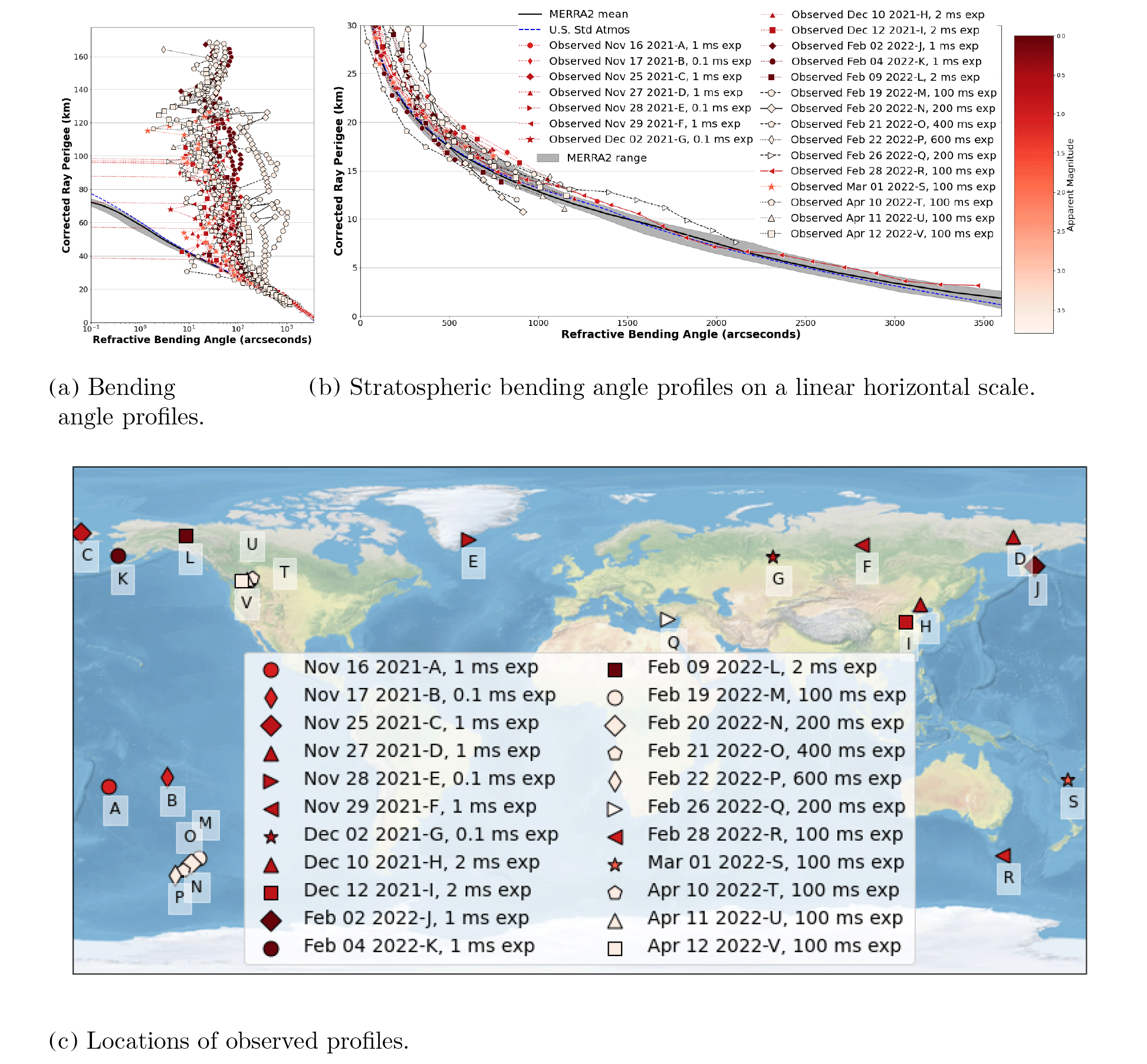
Figure 4 GEOStare SV2 observations in panels (a) and (b) and their locations in panel (c). See Fig. 3 for details. Here the stars captured range from dim to bright with apparent magnitudes 3.6 to −0.04.

Figure 4 shows the location and observed refractive bending angle for the 22 sessions, which profiled a wide range of locations across the globe. Figure 4a and b show the full profile and a zoomed-in stratospheric profile of the GEOStare SV2 observations, respectively. The average location of the ray perigee on the Earth surface is shown in Fig. 4c as circles labeled A–V with the same color as the observations shown in the top panels.

The bending angle profile is calculated with star centroids fit to a 2D Gaussian PSF, and the ray perigee is calculated with the rotated method described in Sect. 2.2.1 and 2.2.3, respectively. Point sources captured by the optics in GEOStare SV2 match a diffraction-limited spot better than the ST optics, so a Gaussian function is a better match for the centroid shape. On the other hand, the uncertainty in image WCS makes calculating the direct ray perigee difficult, so the rotated calculation is used with a reference coordinate taken from the catalog position of the target star.

The data captured here sample the profile more frequently than ST, but the instrument error appears to be significantly higher since the observed bending angle deviates from the MERRA2 and US Standard Atmosphere predictions up to altitudes of 30 km. All sessions are shown in Fig. 4b with dotted lines. We highlight four specific sessions on 19, 20, 21, and 28 February with different line styles. During the 19, 20, and 21 February sessions shown as the black dashed, solid, and dashed lines, respectively, the telescope orientation significantly rotated. The rotation is captured with the payload attitude data, but the frequency of the attitude control system data does not necessarily align with the sampling rate or timing of the captured images and there is significant uncertainty associated with the attitude-derived WCS. The large camera rotation likely caused the significant deviation of the observed bending angle profile from the models. The February 28 session shown as a solid red line successfully observed the atmospheric bending angle as low as 3 km. This session targeted the bright star with apparent magnitude 0.98, Aldebaran, when there were presumably no clouds or objects blocking the star wavefront.

3.3 Retrieved temperature

As shown in Fig. 3a, data collected above 40 km are at too low of a signal-to-noise ratio (SNR) to gather any atmospheric information. Since the retrieval at an altitude z integrates all observations above z, we cut off the observed bending angle at z_max to avoid corrupting the retrieval with too much instrument noise. Figure 5a, b, and c show the final retrieved temperature profile from ST with z_max of 30, 40, and 60 km, respectively. Similarly, Figure 5d, e, and f show the final retrieved temperature profile from GEOStare SV2 with z_max of 20, 30, and 50 km, respectively.

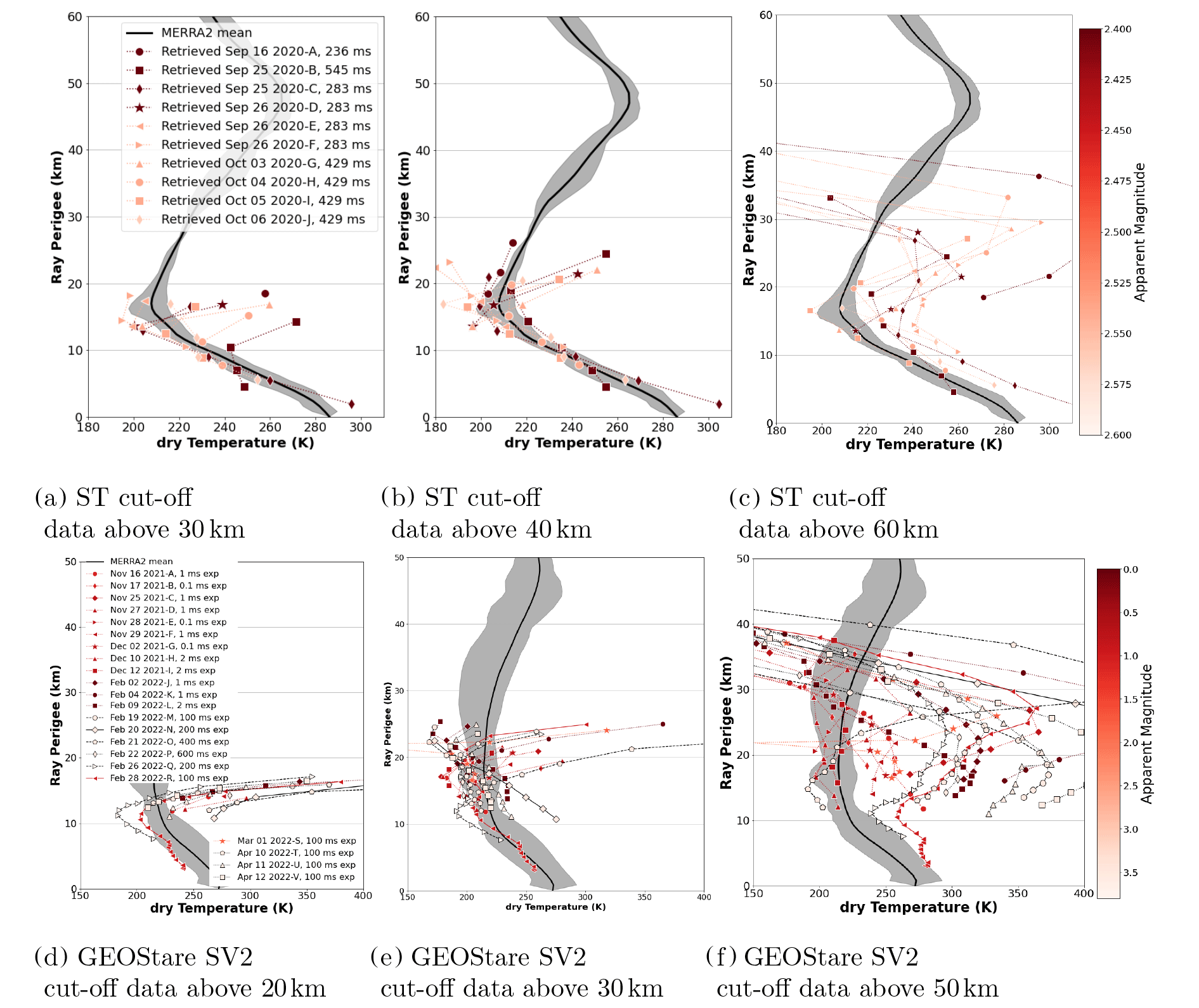
Figure 5 Retrieved temperature profiles from ST and GEOStare SV2 observations. The observation marker shape and color correspond to Figs. 3 and 4 according to the captured star's apparent magnitude shown in the color bars on the right for each measurement dataset. The mean temperature profile predicted by MERRA2 is shown as the black line with the range across the varying measurement locations and dates shown in the gray shaded area.

Figure 5b and e show the best z_max for each instrument: 40 and 30 km for ST and GEOStare SV2, respectively. The left and right panels show cases with too much and too little data removed, respectively. A low cut-off altitude results in too few observations for an accurate retrieval, while a high z_max incorporates too much instrument error in the retrieval. The retrieved temperature profile is accurate at altitudes below 20 km for both of these instruments with the exception of a few datasets (20 and 21 February) that were collected with a rotating field of view. However, the retrieval technique is limited for measurements below 10 km since the impact parameter does not account for refractive index. Future work should address this issue if aiming to retrieve atmospheric conditions below 10 km altitudes.

4 Sounding technique analysis

To assess the proposed atmospheric sounding technique, we utilize the refraction forward model described in Sect. 2.1 based on the Naval Research Laboratory empirical atmospheric model NRLMSISE0 (Emmert et al., 2021) over the Pacific Ocean. The modeled refractive bending angle is sampled at 500 m vertical resolution, and noise is added to simulate satellite measurements. Then, the retrieval technique described in Sect. 2.3 is applied to the simulated noisy measurements and compared with the NRLMSISE0 temperature profile to analyze how well the sounding technique can estimate the stratospheric temperature profile.

4.1 Measurement error

Measurement error in the bending angle is due to uncertainty in the centroid position since it is calculated from the distance between the observed star centroid and its reference centroid position. The centroid position uncertainty σ_x in pixels is characterized with uncertainty due to background signal σ_bkd, photons captured from the source signal σ_signal, atmospheric turbulence σ_turb, and boresight pointing σ_BS (Thomas et al., 2006).

$$\begin{array}{}\text{(11)}& {\mathit{\sigma }}_x=\sqrt{{\mathit{\sigma }}_{\mathrm{bkd}}^{\mathrm{2}}+{\mathit{\sigma }}_{\mathrm{signal}}^{\mathrm{2}}+{\mathit{\sigma }}_{\mathrm{turb}}^{\mathrm{2}}+{\mathit{\sigma }}_{\mathrm{BS}}^{\mathrm{2}}}\end{array}$$

The centroid error due to background signal depends on the spot size described by its full-width half-maximum (FWHM), the spot strength based on the number of photons captured N_ph, and the background strength in terms of the number of photons across the spot N_bkd. Any centroid blurring due to jitter of the spacecraft is captured by the estimated spot size FWHM. The centroid signal N_ph is based on the star apparent magnitude, the exposure time, the efficiency and transmission of the optical system, refractive attenuation (Gurvich and Brekhovskikh, 2001; Sofieva et al., 2007), and transmission loss due to Rayleigh scattering. The background signal of the sky and airglow is estimated from the measured intensity in ADU s⁻¹ per pixel, the camera inverse gain in electrons per ADU, the exposure time, and the spot size.

The centroid uncertainty σ_signal increases as the source signal and N_samp decrease. N_samp represents the number of pixels sampled by a diffraction-limited spot based on the plate scale p, light wavelength λ, and the aperture diameter D_aper.

Turbulence impacts the centroid by blurring the spot during the camera integration timeframe if the turbulence is strong enough. The turbulence strength is characterized by the Fried parameter r₀ cm (Fried, 1965), which is defined as the required aperture diameter to resolve atmospheric turbulence. Perlot (2009) describes the $\mathrm{5}/\mathrm{7}$ Hufnagel–Valley model (HV${}_{\mathrm{5}/\mathrm{7}}$) we use for a typical atmospheric turbulence vertical profile. Thomas et al. (2006) describe the effect of turbulence based on an empirical parameter K, the window size, Fried parameter, and aperture diameter.

Uncertainty in the boresight pointing directly propagates to the centroid uncertainty with σ_BS.

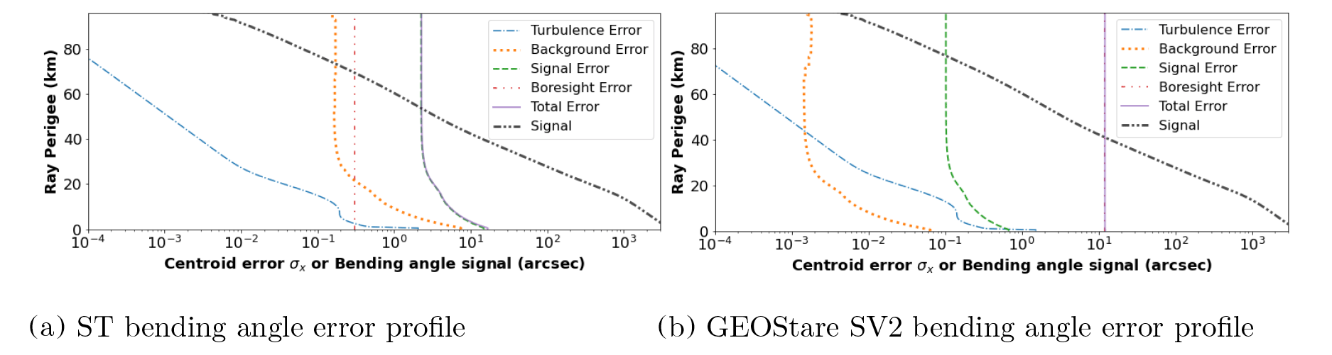
Figure 6 Bending angle error analysis for each satellite. The thick, dash–dot-dotted black line shows the expected bending angle. The blue dash-dotted, orange dotted, green dashed, and thin red dash–dot-dotted lines show the uncertainty in centroid position due to atmospheric turbulence, background signal, photon signal and centroiding, and satellite pointing, respectively. The total uncertainty in the centroid position is shown with the purple solid line.

Based on the details of each satellite and telescope configuration, we estimate the measurement error vertical profile. The equations and parameters used for each instrument are described in the Appendix and in Sect. 3 assuming each set-up utilizes one of the dimmer stars captured during the actual data collections corresponding to Markeb and Algedi for ST and GEOStare SV2, respectively. This corresponds to a 2.5 and 3.57 apparent magnitude star, respectively, and integration time of 430 and 100 ms, respectively. Applying the details of each instrument to the centroid uncertainty, the bending angle error and its components are shown in Fig. 6 for ST and GEOStare SV2 along with the expected bending angle, or measurement signal, for reference.

The signal and background errors depend on N_ph, the star brightness, and as light passes deeper into the atmosphere there is transmission loss due to Rayleigh scattering and refraction that dims the observed star. Therefore, these sources of uncertainty grow towards the Earth's surface in the lower stratosphere and troposphere. The background signal also slightly increases near the airglow at 80–100 km and below as the sky brightness increases. GEOStare SV2 has a much lower background signal due to its design to keep stray light from the telescope. This analysis shows that the star brightness and uncertainty in the boresight are the most significant sources of uncertainty in ST and GEOStare SV2 data, respectively.

4.2 Retrieval analysis

To evaluate our retrieval technique, we simulate noisy satellite measurements by corrupting the modeled bending angle sampled at 0.5 km resolution with white noise scaled by the centroid uncertainty profile. Then, the retrieval method described in Sect. 2.3 is applied to the section of simulated bending angle measurements with a signal-to-noise ratio (SNR) of at least 2. The altitude corresponding to an SNR of 2 is the data cut-off altitude. However, there is still error in the retrieved temperature compared to the true temperature profile near the upper and lower sections of the profile, even with an SNR above 2. Therefore, we assess the retrieval cut-off altitude by determining the level (above 10 km) below which the percent error is below 2 %, so the retrieved temperature error is below a 2 % threshold between the retrieval cut-off and 10 km; 2 % is the threshold for being precise enough to detect atmospheric gravity waves.

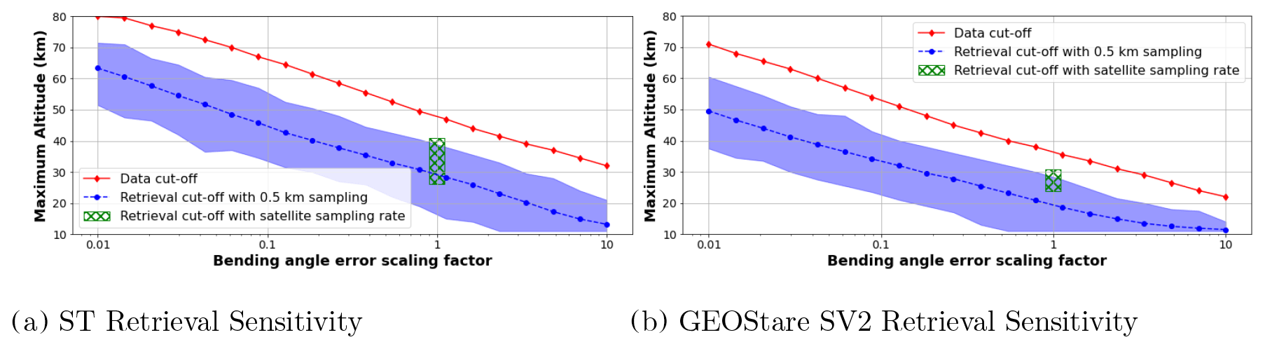
Figure 7 Maximum altitude of retrieved atmospheric sounding profile analysis for each satellite measurement. The red diamonds show the data cut-off due to a degraded SNR relative to the amount of added bending angle noise. The maximum altitude according to a threshold of 2 % error in retrieved temperature is shown with the mean and range of the ensemble in blue circles and blue shaded area, respectively. The maximum altitude of 10 % error in retrieved temperature utilizing the observed vertical resolution is shown in the green hatched area for the lowest to highest vertical resolution of each instrument.

The above retrieval analysis is performed for the instrument nominal case and several other cases with the bending angle error scaled by a factor from 0.01 to 10. For each bending angle error scaling factor, we simulated 1000 realizations of the noisy measurements by calculating the cut-off altitudes for each scenario, and the average result is shown here. The data cut-off z_max and mean retrieval cut-off are shown in Fig. 7 with solid red diamonds and dashed blue circles, respectively. Additionally, the range in the retrieval cut-off among the ensemble of 1000 scenarios is shown in the blue shaded region. The result for ST data is shown in Fig. 7a with higher cut-off altitudes than GEOStare SV2 data shown in Fig. 7b due to its lower nominal bending angle error.

This analysis shows the theoretical performance of each instrument across limiting cases: (1) if aspects of the measurements are improved resulting in a factor of 100 lower bending angle error; (2) if the measurement is degraded so the error is enhanced by a factor of 10. The worst-case scenario simulated with the GEOStare SV2 set-up and the bending angle error degraded by a factor of 10 results in a noise floor of 121 arcsec. In this case, 55 % of the noisy measurement realizations provide retrieved temperature within the error threshold of 2 %, and the remainder only retrieve up to 11.5 km on average. In contrast, with a scaling factor of 0.03 on the ST instrument, the mean bending angle error is similar to the current background error of approximately 0.07 arcsec. This scenario results in retrieved temperature from 10 km up to 42–64 km with an average maximum altitude of 55 km.

This analysis does not reproduce retrievals from the satellite measurements since the atmosphere was sampled at a frequency of 0.5 km and the real observations were sampled with spacing between 1.5 and 8 km. The lower sampling rate results in poor-quality retrievals with the Abel inversion technique, so to assess the real observation system we use a threshold of 10 % temperature error instead of 2 %. The data cut-off for the lower sampling rate is approximately the same as the higher sampling rate shown in the red diamond at a scaling factor of 1 in Fig. 7. The ranges in retrieval cut-off for a sampling rate between 3–8 and 1.5–6.5 km for ST and GEOStare SV2, respectively, are shown in green hatched regions in Fig. 7.

5 Future observations

A future instrument, Stellar Occultation Hypertemporal Imaging Payload (SOHIP), was planned to launch in January 2023, joining the suite of instruments on the International Space Station. SOHIP can be leveraged to achieve a higher SNR since it includes the high-resolution camera of GEOStare SV2 with an even higher frame rate along with a second telescope somewhat similar in size to a Terran Orbital star tracker. Operating two telescopes in tandem will mitigate the trade-off discussed above between σ_BS and σ_signal when choosing an integration time.

The star tracker camera on board SOHIP can capture a large field of view with a long integration time to reduce the boresight error from σ_BS=12 arcsec observed with GEOStare SV2 to σ_BS=0.3 arcsec when determining an astrometric solution. The high-resolution “science” telescope on board SOHIP has the same design and specifications as the GEOStare SV2 telescope, so σ_bkd is below 0.01 arcsec. The goal of SOHIP is to observe a high-vertical-resolution profile with the stellar occultation methodology, so the science telescope will operate with a high frame rate near 1 kHz and thus a short integration time. This limits the targets to only the brightest stars, and the σ_signal is 0.2 arcsec, similar to GEOStare SV2 due to the short integration. Additionally, a 1 kHz frame rate results in a vertical sampling rate of approximately 3 m depending on the viewing angle.

This overall design results in a more accurate bending angle measurement with σ_x of 0.39 arcsec. This noise floor corresponds to a maximum retrieval altitude between 30 and 50 km based on a 2 % error threshold in temperature (41 km maximum altitude on average). Additionally, the accuracy and precision of retrieved temperature at 25 km are predicted to be 0.5 and 0.7 K, respectively (not shown).

6 Conclusions

The technique and observations presented here serve as proof of concept for utilizing nanosatellites for stellar occultation measurements for atmospheric sounding. Stellar occultation captures an optical wavefront as the starlight passes through the atmosphere, adjusting the apparent centroid position based on the atmospheric refractivity. We observe a vertical profile of the atmospheric refractive bending angle, which allows us to retrieve atmospheric refractivity, density, and temperature profiles.

We present data gathered from two types of on-orbit sensors: a dedicated imaging telescope on the GEOStare SV2 mission and data collected from ST sensors. Both instruments result in significant uncertainty so that the highest altitude of observed bending angle is 30 km. ST observations are limited by the relatively low-resolution sensor, but the long exposure and large field of view enabled an accurate estimate of the telescope pointing coordinates and orientation. On the other hand, GEOStare SV2 is limited by the error in attitude-derived telescope pointing, not due to satellite stability but the mode of data collection with short integration times even though the instrument has a high-resolution camera and sampling rate.

Simulated measurements based on the known source of uncertainty contributing to the bending angle agree with the observed signal-to-noise ratio (SNR). We find that the profile can be extended from an upper limit of 20 km if the overall error is decreased by a factor of 100 for ST or GEOStare SV2 up to 60 km or 50 km, respectively, assuming 2 % error in retrieved temperature. An upcoming 2023 SOHIP mission is expected to retrieve temperature up to 41 km on average and a precision of 0.7 K at 25 km with a high vertical sampling near 3 m. This is due to utilizing both a star tracker and GEOStare SV2 sensor to detect atmospheric gravity waves.

This technique is a promising, inexpensive method to observe the stratospheric temperature profile and potentially observe small-scale perturbations in the atmospheric field. The small optical wavelengths captured with stellar occultation allow the observation of small-scale upper atmosphere phenomena like atmospheric gravity waves and turbulence. This method can lead to a remote observation method able to probe sections of the atmosphere where turbulence currently cannot be detected or measured, which is relevant for future supersonic airliners. A future instrument, SOHIP, aims to achieve this by utilizing two cameras capturing a bright star with both a long and short exposure time, providing high-SNR bending angle observations.

Appendix A: Definitions and physical constants used

texp	exposure time (s)
m	apparent magnitude of star
Ibkd(z)	intensity of background signal in night sky at ray perigee z (ADU s−1 per pixel)
𝒢	inverse gain of detector ($e^{-}/\mathrm{ADU}$)
FWHM≊2	pixels – full-width half-maximum of source
Npix≊FWHM2	number of pixels subtended by star
Nsamp	half-width of diffraction-limited spot (pixels)
rn	electrons of read noise; $N_r^{\mathrm{2}}$ read-out noise variance
p	plate scale in pixel per radian
σx	uncertainty in source position in arcsec
Aaper	Aperture area from diameter Daper=8.5 cm
Qe & fopt	Quantum efficiency and transmission of optical system (0.7 & 0.9, resp)
BW	bandwidth (3000 Å)
F0	Vega photon flux in R band (600 photon cm−2 s−1 Å−1)
fscat(z)	fraction of signal transmitted (due to Rayleigh scattering at 400 nm wavelength) at ray perigee z
q(z)	refractive attenuation (or dilution) at ray perigee z
λ	wavelength (0.7 µm)
K	coefficient for turbulence effect on centroid (0.5 pixel2)
Wpix:=FWHM	window length (2 pixels)
r0	Fried parameter (cm)
σBS	uncertainty in boresight pointing (pixels)
δ	FWHM of Gaussian spot (pixels)
$C_N^{\mathrm{2}}$	turbulence strength parameter (m${}^{-\mathrm{2}/\mathrm{3}}$)
ζ	zenith angle (radians)

Appendix B: Instrument error

The centroid uncertainty σ_x is determined with the following equations.

$$\begin{array}{}\text{(B1)}& {\displaystyle }\mathit{\delta }=\mathrm{FWHM}/\sqrt{\mathrm{2}}\text{(B2)}& {\displaystyle }{N}_{\mathrm{ph}}=F_{\mathrm{0}}\mathrm{BW}{A}_{\mathrm{aper}}{\mathrm{2.512}}^{-m}{t}_{\exp }{Q}_{\mathrm{e}}{f}_{\mathrm{opt}}{f}_{\mathrm{scat}}\left(z\right)q\left(z\right)\text{(B3)}& {\displaystyle }{N}_{\mathrm{samp}}={\displaystyle \frac{p\mathit{\lambda }}{D_{\mathrm{aper}}}}\text{(B4)}& {\displaystyle }{N}_r=\sqrt{N_{\mathrm{pix}}{r}_{\mathrm{n}}^{\mathrm{2}}}\text{(B5)}& {\displaystyle }{N}_{\mathrm{bkd}}=\sqrt{\mathcal{G}{I}_{\mathrm{bkd}}\left(z\right)N_{\mathrm{pix}}{t}_{\exp }}\text{(B6)}& {\displaystyle }{r}_{\mathrm{0}}\left(z\right)=\mathrm{100}\times {\left[\mathrm{0.423}(\mathrm{2}\mathit{\pi }/\mathit{\lambda }{)}^{\mathrm{2}}\underset{z}{\overset{\mathrm{100}}{\int }}\sec \mathit{\xi }(h\left)\mathrm{d}h{C}_N^{\mathrm{2}}\right(h)\right]}^{-\mathrm{3}/\mathrm{5}}\text{(B7)}& {\displaystyle }{\mathit{\sigma }}_x=p^{-\mathrm{1}}\sqrt{{\displaystyle \frac{\mathrm{4}{\mathit{\delta }}^{\mathrm{2}}{N}_{\mathrm{bkd}}^{\mathrm{2}}}{N_{\mathrm{ph}}^{\mathrm{2}}}}+{\displaystyle \frac{{\mathit{\pi }}^{\mathrm{2}}}{\mathrm{2}\ln \left(\mathrm{2}\right)N_{\mathrm{ph}}}}{\displaystyle \frac{{\mathrm{FWHM}}^{\mathrm{2}}}{N_{\mathrm{samp}}^{\mathrm{2}}}}+K{\left(W_{\mathrm{pix}}{\displaystyle \frac{D_{\mathrm{aper}}}{p\mathit{\lambda }}}\right)}^{-\mathrm{2}}{\left({\displaystyle \frac{D_{\mathrm{aper}}}{r_{\mathrm{0}}\left(z\right)}}\right)}^{\mathrm{5}/\mathrm{3}}+{\mathit{\sigma }}_{\mathrm{BS}}^{\mathrm{2}}}\end{array}$$

Appendix C: Supplemental figures

The observed bending angle by star tracker matches the MERRA2 model better than the US Standard Atmosphere, as shown in Fig. C2 with a parity plot between the observations and the two reference models. The blue circles represent the comparison of the data with MERRA2, while the red diamonds show the comparison with the US Standard Atmosphere, resulting in correlation coefficients of 0.986 and 0.983, respectively. The MERRA2 model is much more accurate since it is a global reanalysis model actively developed, so observations correlating with MERRA2 better than the US Standard provides confidence in these measurements.

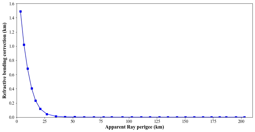
Figure C1 Correction to ray perigee to account for refractive bending with ray-tracing algorithm.

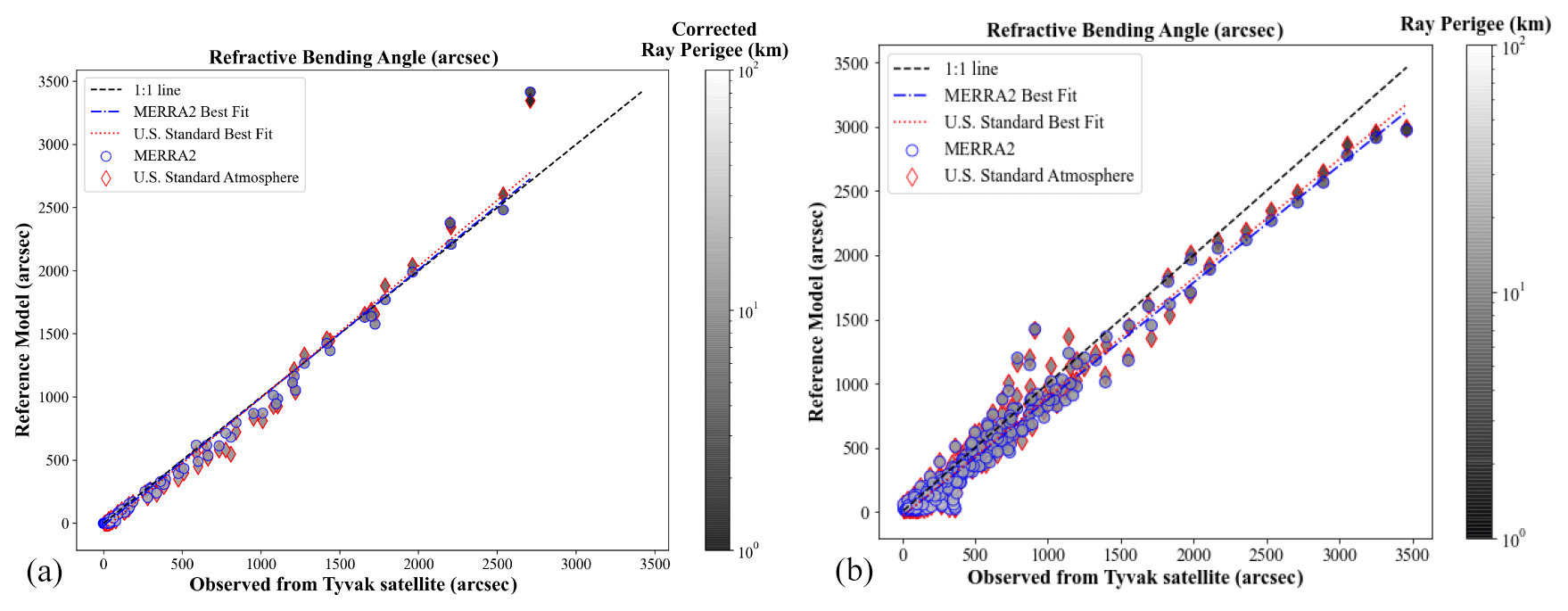
Figure C2 Parity plot of the US Standard and MERRA2 reference model predictions against the observed bending angle from star tracker and GEOStare SV2 in panels (a) and (b), respectively. The ray perigee of each point is shown in the grayscale color bar.