Reconstruction of high-frequency methane atmospheric concentration peaks from measurements using metal oxide low-cost sensors

Detecting and quantifying CH₄ gas emissions at industrial facilities is an important goal for being able to reduce these emissions. The nature of CH₄ emissions through “leaks” is episodic and spatially variable, making their monitoring a complex task; this is partly being addressed by atmospheric surveys with various types of instruments. Continuous records are preferable to snapshot surveys for monitoring a site, and one solution would be to deploy a permanent network of sensors. Deploying such a network with research-level instruments is expensive, so low-cost and low-power sensors could be a good alternative. However, low cost usually entails lower accuracy and the existence of sensor drifts and cross-sensitivity to other gases and environmental parameters. Here we present four tests conducted with two types of Figaro^® Taguchi gas sensors (TGSs) in a laboratory experiment. The sensors were exposed to ambient air and peaks of CH₄ concentrations. We assembled four chambers, each containing one TGS sensor of each type. The first test consisted in comparing parametric and non-parametric models to reconstruct the CH₄ peak signal from observations of the voltage variations of TGS sensors. The obtained relative accuracy is better than 10 % to reconstruct the maximum amplitude of peaks (RMSE ≤2 ppm). Polynomial regression and multilayer perceptron (MLP) models gave the highest performances for one type of sensor (TGS 2611C, RMSE =0.9 ppm) and for the combination of two sensors (TGS 2611C + TGS 2611E, RMSE =0.8 ppm), with a training set size of 70 % of the total observations. In the second test, we compared the performance of the same models with a reduced training set. To reduce the size of the training set, we employed a stratification of the data into clusters of peaks that allowed us to keep the same model performances with only 25 % of the data to train the models. The third test consisted of detecting the effects of age in the sensors after 6 months of continuous measurements. We observed performance degradation through our models of between 0.6 and 0.8 ppm. In the final test, we assessed the capability of a model to be transferred between chambers in the same type of sensor and found that it is only possible to transfer models if the target range of variation of CH₄ is similar to the one on which the model was trained.

1 Introduction

Methane (CH₄) is a greenhouse gas 28 times more potent than carbon dioxide, considering its warming potential over 100 years (Travis et al., 2020). Anthropogenic CH₄ emissions account for 60 % of global emissions (Saunois et al., 2020). Emissions from natural-gas production account for 63 % of total emissions in the category of fossil fuel production and use (Saunois et al., 2020). Fugitive leaks of natural gas at industrial facilities also present a safety hazard. Emissions from such facilities need to be continuously monitored, due to the episodic and spatially variable nature of leaks (Coburn et al., 2018). Leaks can be detected and quantified by LDAR (Leak Detection And Repair) surveys to detect high concentrations caused by a leak. Those surveys are periodical and have limitations related to the portability of instruments or accessibility of sites. A possible solution to overcome these limitations is to deploy a network of sensors that continuously measure methane concentrations around an emitting area (Kumar et al., 2015). Deploying such a network with highly precise instruments, using techniques such as cavity ring-down spectrometry (CRDS) is, however, cost-prohibitive. Low-cost sensors such as low-power metal oxide semiconductor (MOS) sensors for methane are an alternative. Recent studies (Riddick et al., 2020; Casey et al., 2019; Collier-Oxandale et al., 2018; Jørgensen et al., 2020; Rivera Martinez et al., 2021; Eugster et al., 2020) tested the ability of MOS sensors to monitor methane concentrations in natural and controlled conditions and showed a fair agreement between the concentrations derived from the sensors and those from high-precision reference instruments. MOS sensors are composed of a semiconducting-metal-oxide-sensing element heated at a temperature between 20 and 400 ^∘C (Örnek and Karlik, 2012; Barsan et al., 2007). When the semiconducting material is in contact with an electron donor gas like CH₄, a change in the conductivity occurs, measured by an external electrical circuit (Örnek and Karlik, 2012). MOS sensors are known to be less precise than CRDS to CH₄ variations, although they can detect small variations in concentrations. Most MOS sensors have cross-sensitivities to other electron donors and to environmental variables such as absolute humidity, pressure and temperature (Popoola et al., 2018), with non-linear interactions (Rivera Martinez et al., 2021).

Biases affect CH₄ measurements derived from low-cost sensors because of cross-sensitivities to other gases, dependence on environmental factors and internal drifts, e.g., due to aging. Figaro^® Taguchi gas sensors (TGSs) are a particular series of MOS capable of measuring CH₄. In order to limit biases of these sensors, several studies proposed a calibration model against a high-precision reference instrument. Casey et al. (2019) compared different calibration approaches with inverse and direct linear models and artificial neural networks to quantify O₃ from an SGX Corporation MiCS-2611 sensor, CO from a Mocon Baseline photoionization detector (PID) sensor, CO₂ from an ELT S-100 non-dispersive infrared (NDIR) sensor and CH₄ from observations of a Figaro^® TGS 2600 sensor. Collier-Oxandale et al. (2018, 2019) applied multilinear models, including interactions from environmental variables, to predict CH₄ concentrations and to detect and quantify volatile organic compounds (VOCs) from Figaro^® TGS 2600 and TGS 2602 MOS sensors at two sites with active oil and gas operations. Eugster et al. (2020) used empirical functions and artificial neural networks (ANNs) to derive CH₄ concentrations from 6 years of data collected with Figaro^® TGS 2600 sensors at a field site in the Arctic. Riddick et al. (2020) derived nonlinear empirical relationships for Figaro^® TGS 2600 sensors from three experiments, with durations varying from 1 d to 1 month. Rivera Martinez et al. (2021) reconstructed CH₄ concentration variations in room air from Figaro^® TGS 2611-C00 sensors using ANN models and co-variations of temperature, water mole fraction and pressure. Nevertheless, those comparisons were limited by the choice of a specific reconstruction model and restricted to only one type of sensor.

There is a need for a more thorough comparison of different calibration approaches for Figaro^® MOS sensors applied to measure CH₄. In addition, there is a need to assess the performances of MOS sensors to detect and quantify CH₄ spikes typical of industrial emission. This study aims to compare several parametric (linear and polynomial) and non-parametric models (random forest, hybrid random forest and ANNs) applied to different combinations of Figaro^® TGS sensors to reconstruct the CH₄ signals of repeated atmospheric spikes, based on the observed voltage of each sensor and environmental variables such as air temperature and pressure and H₂O mole fraction. The CH₄ signal we aim to reconstruct is representative of variations observed in the atmosphere from leaks that occur within or close to an emitting industrial facility, i.e., short-duration CH₄ enhancements (spikes) lasting between 1 and 7 min and ranging from a few tenths of parts per million to a few parts per million above an atmospheric background concentration of around 2 ppm (Kumar et al., 2021). In this study, we performed a laboratory experiment where a CRDS instrument and many TGS sensors of different types were exposed to a controlled airflow with artificially created CH₄ concentration spikes (Sect. 2). The spikes were composed of pure CH₄ and did not contain any VOCs, although those species could be present in natural-gas leaks from oil and gas facilities. The main focus of this study is the behavior of TGS sensors that are exposed to enhancements of CH₄ on top of a background signal without the presence of other interfering gases. The influence of VOCs on a real deployment should be considered and included as a predictor to the reconstruction models, corrected on a preprocessing stage by determining the sensitivity of TGS to them or determining, from specific laboratory experiments, the amount of signal that models can filter out and the needs in terms of ancillary measurements. The experiment lasted 4 months and provided 838 spikes, which give us a dense and complex dataset to train and test different models for reconstructing CH₄ variations.

For low-cost sensors, a collocation is often required with a highly precise reference instrument to train an empirical calibration model. This training phase should be as effective (parsimonious) as possible. The strategy is to reduce the time and maintenance costs of having a reference instrument on site if the purpose is to bring it in the field for future studies where low-cost sensors would have to be calibrated. We investigate the problem of “parsimonious training” by testing different configurations (model and inputs) to establish the minimum amount of reference data needed to obtain good performances with low-cost sensors (Sect. 3.2 and 3.3). Secondly, since the performance of low-cost sensors may change with time, it is important to understand if their measurements could be affected by a drift of their sensitivity over time. We address this problem of “non-stationary training” by comparing different calibration models for a second spike experiment conducted 6 months after the first one (Sect. 3.4). Thirdly, sensitivities may vary from one sensor to another and may require a sensor-specific calibration model, which becomes a problem when a large number of sensors are deployed. Finding a robust calibration model that could be trained using data from one or several sensors and applied to others remains an open question. We bring some insight to this problem of “generalized calibration” by training models to reconstruct the CH₄ signal from a group of sensors located in the same chamber and applying them to other groups of sensors in a different chamber (Sect. 3.5). To assess the performance of the calibration models and particularly their capability to reconstruct spikes of several parts per million occurring upon a background CH₄ level, here we define an acceptable performance to be an error of less than the 10 % of the maximum amplitude of the peaks we aim to reconstruct. In our case, this requirement is an RMSE of 2 ppm between the reconstructed CH₄ data from low-cost sensors and the true data from a reference instrument at a time resolution of 5 s.

2 Methods

2.1 Experimental setup

2.1.1 Low-cost CH₄ sensors

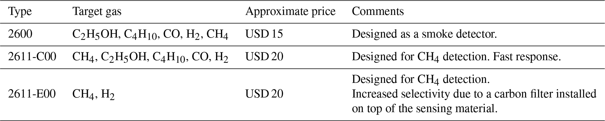
For the experiment, four independent sampling chambers were assembled. Each chamber contained a Figaro^® TGS 2600 originally designed to measure VOCs but sensitive to CH₄, TGS 2611-C00 with enhanced sensitivity to CH₄ and TGS 2611-E00 that includes a carbon filter on top of the sensing material to improve the selectivity to CH₄ even further (see Table A7 for information on the differences of each TGS sensor), alongside a relative humidity and temperature sensor (DHT22 or Sensirion SHT75), and a temperature and pressure sensor (Bosch BMP280; see Table 1 for details). Issues with the logger system produced gaps in environmental variables data, thus observations information from an external chamber (E; see Fig. 1b and Table 1 for details) was used in the correction of the sensitivity across all chambers. The sensors were placed on a circuit board to minimize the direct heating influence of the TGS sensors on temperature measurements. The sampling chamber was made of acrylic/glass with a gas inlet and outlet and a port for the electrical cables (Fig. 1a). Each sensor was connected in series with a high-precision load resistor which controlled sensitivity (Figaro, 2013, 2005). The voltage across each load resistor was recorded by an AB Electronics PiPlus ADC board, mounted on a Raspberry Pi 3b+ logging computer, and sampled at a frequency of 0.5 Hz (2 s). This voltage measurement was used in our characterization algorithms, referred to hereafter as the sensor voltage. We focus on the reconstruction of CH₄ using only the TGS 2611-C00 and TGS 2611-E00 data.

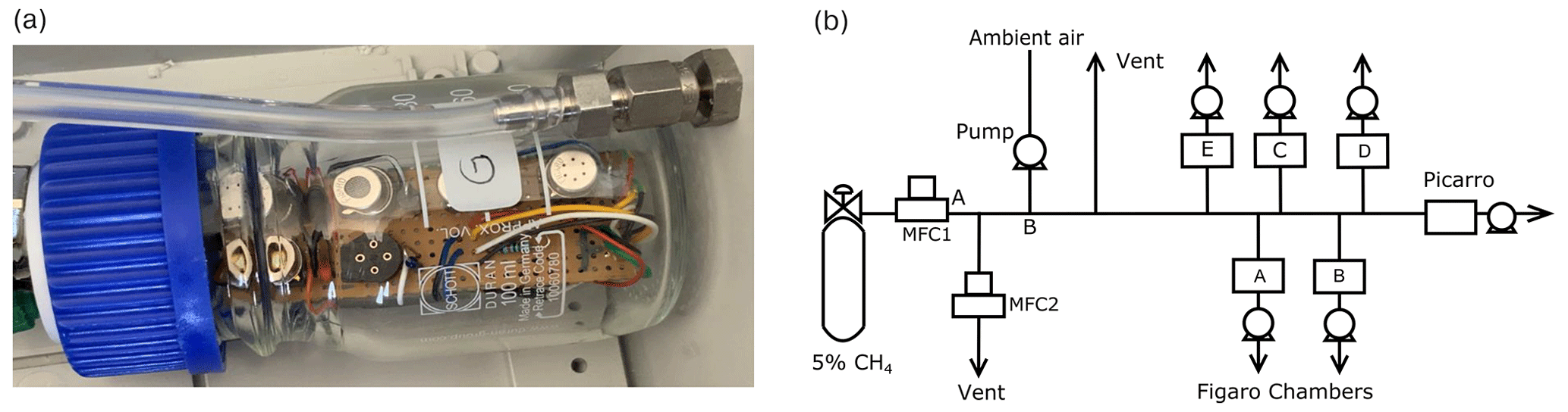
Figure 1 (a) Example of a chamber with three sensors inside. (b) Scheme of the spike creation experiment.

Table 1 Summary of the sensors included on each logger box.

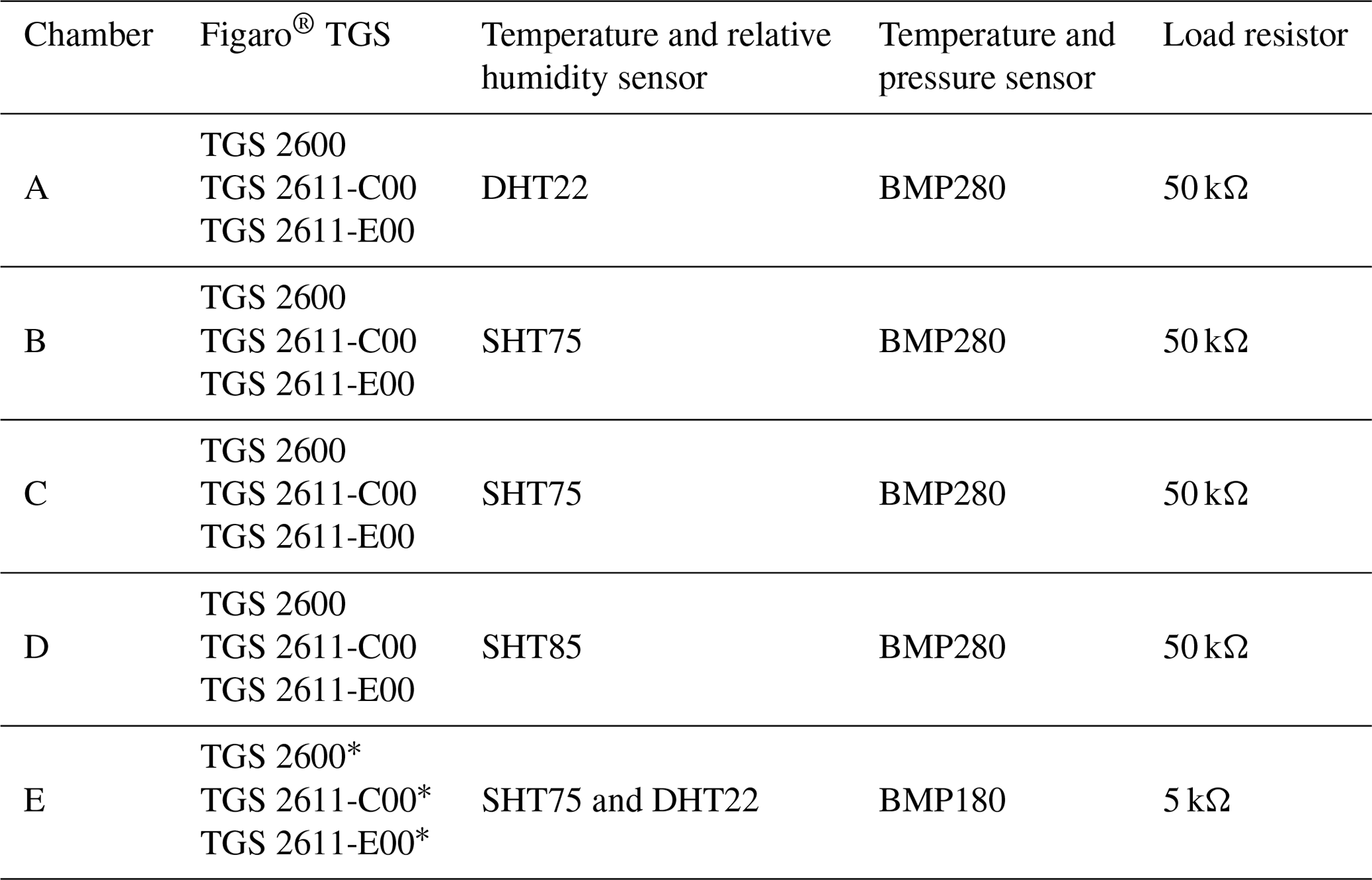
^* Two sensors of this type.

2.1.2 Generation of methane spikes on top of ambient air

The experiment lasted 130 d from 28 October 2019 to 5 March 2020. During this period, the six chambers containing TGS sensors sampled ambient air pumped from the roof of the laboratory. Relative humidity, air pressure and temperature were measured in the ambient air flux, as well as CH₄, using a Picarro CRDS G2401 reference instrument. No calibration was considered on the CRDS instrument during the experimental period due to its high precision and low drift over time (less than 1 ppb per month; Yver-Kwok et al., 2015).

To expose the TGS sensor chambers to CH₄ enhancements (spikes) of different durations and amplitude comparable with typical enhancements observed around industrial sites (Kumar et al., 2021), we designed an automatic system to add small amounts of CH₄ on top of the ambient air acquired from our roof. The system presented on Fig. 1b consists of an ambient airflow to which a small amount of a gas was periodically added from a cylinder containing 5 % of CH₄ (in argon), controlled by two mass flow controllers denoted MFC1 and MFC2 in Fig. 1b.

The occurrences of the spikes were programmed to be automatically generated, with at least three spikes each day. The duration and magnitude of the spikes were predefined and controlled by varying the flows of MFC1 and MFC2, the two mass flow controllers that were programmed to add an amount of CH₄ to produce spikes of an expected amplitude ranging between 3 and 24 ppm. Two different types of spikes were generated. The first type, with large amplitudes between 20 and 24 ppm, was generated from 28 October to 9 December 2019. The second type, with smaller amplitudes ranging between 5 and 10 ppm but with a higher number of spikes during a given period of time, was generated from 9 December 2019 to 5 March 2020. The typical duration of the spikes of both types varied between 1 and 7 min, which is longer than the known response time of the TGS sensors. Gas from the 5 % CH₄ cylinder that persisted on the airflow after a spike in segment A–B (Fig. 1b) was expulsed though MFC2, preventing very high CH₄ concentrations to remain in the airflow following a spike. We verified that the amount of gas with 5 % of CH₄ added to the airflow measured by the TGS sensors did not affect the air pressure, temperature and relative humidity in the chambers.

The volume of each chamber is 100 mL, and the flow rate through the chambers was fixed to 2.5 L min⁻¹. We did not test the effect of increasing the flow rate on the TGS measurements. Instead, we decided to choose a high enough flow rate to reduce the buffering effect of the chamber volume that would systematically smooth the CH₄ spikes. Despite this setup, a buffering effect was still present in the chamber, evidenced by the fact that after stopping the injection of air with 5 % CH₄, the CH₄ drawdown in the chamber was observed to be smooth and lagged the drawdown of the CRDS instrument by a time constant of 10 s, consistent with previous measurements on buffer volumes acting as a low-pass filter (Cescatti et al., 2016).

To determine the time constant (τ) of the buffer effect of the chambers, we applied an exponential weighted moving average to the CRDS data with different values of τ and compared them with the shape of the response of the TGS sensor (see Fig. A1). The time constant applied on the reference instrument to compare both TGS sensor types is the same. A similar approach was employed by Jørgensen et al. (2020) to compensate for effects of microturbulent mixing of subglacial air with atmospheric observations. Before applying this temporal smoothing on the CRDS data, we resampled both signals, the reference CRDS and the TGS, from their original time resolutions (1 and 2 s, respectively) to a common time resolution of 5 s. The time shift due to incorrect clock synchronization between the reference CRDS instrument and the loggers of the TGS sensors was partly corrected with a search of the maximum correlation on non-overlapping windows of 6 h and a manual inspection of the agreement between TGS voltages and CH₄ observations of the reference CRDS instrument.

2.2 Separating CH₄ spikes from background variations in ambient air

Different algorithms have been proposed to identify short-term variations of atmospheric signals (Ruckstuhl et al., 2012) from slower variations of background variations in atmospheric composition. These approaches were applied to low-cost sensors for the detection of local events (Heimann et al., 2015) and for the removal of diurnal periodical signals to identify peaks of air pollutants (Collier-Oxandale et al., 2020). In this study, we want to separate the background of slowly varying CH₄ in the outside air pumped from the laboratory roof from the signal of the CH₄ spikes by using an algorithm.

We followed a three-step approach. The first step was to remove the impact of H₂O variations on the sensor voltage signals, given that H₂O changes in the background air. Previous studies (Eugster and Kling, 2012; Rivera Martinez et al., 2021) demonstrated a direct dependence between the voltage/resistance of metal oxide sensors and the H₂O concentration. In order to determine this relationship, we used the background H₂O mole fraction and TGS voltage measurements in ambient air during a period of 32 d with no CH₄ spikes and regressed both variables to derive the H₂O sensitivity of the voltage of each TGS sensor (in mV per ppm H₂O). This linear model of the voltage–H₂O sensitivity was applied to voltage time series of the TGS sensors during the spike measurement period.

The second step was to separate background and spike conditions from voltage variations in the time series. We tested two approaches. The first approach applied the peak detection algorithm of Coombes et al. (2003) to detect the voltage associated with spikes and separate the background signal by a linear interpolation between non-spike values at the start and the end of each spike. The second approach applied the robust extraction of baseline signal (REBS) algorithm from Ruckstuhl et al. (2012) to separate voltage observations associated with background from those during the spikes. The principle of REBS is to compute local regressions over the time series on small moving time windows (60 min) and to iteratively identify outliers that are far from the modeled background, based on a threshold. Here, the detected outliers are considered to belong to a spike. The threshold or scale parameter, β, defines a range in the number of standard deviations around the modeled baseline. A value of β=3.5 ppm was used. The third step was to remove observations corresponding to the baseline and only keep the data classified as spikes, which form the signal of interest in this study.

2.3 Modeling CH₄ spikes from TGS sensor voltages and environmental variables

The impact of different magnitudes of the variables used as predictors is prone to affecting the parameters of the models in the training stage. Thus, to reduce this impact, we standardize the inputs before training the models. We chose a robust scaler unaffected by outliers by removing the median and scaling the data to a quantile range (Demuth et al., 2014). To reconstruct CH₄ spikes from TGS sensor voltages, we applied linear and polynomial regressions, ANNs and random forest models, all trained using the CRDS measurements. We assessed the performance of the different models using a k-fold cross-validation, here with k=20. A fraction of the data was used for the training of each model and the rest for evaluation. We repeated this training and evaluation process with a moving window to make a robust assessment of each model performance considering all data available. We specified two cases for the relative sizes of the training and evaluation (test) sets. The first case used training and test set fractions of 70 % and 30 % of the observations, respectively, and the second one used 50 % and 50 %. We focus in the example below on the spike data from one chamber (chamber A) using different models as test inputs: (1) voltages of TGS C or E sensors separately; (2) voltages of a single sensor type and measurements of H₂O, temperature and pressure; (3) combined TGS C and E voltages; and (4) combined TGS C and E voltages, as well as H₂O, temperature and pressure.

2.3.1 Linear and multilinear regression models

Linear regressions between dry-air CH₄ concentrations from the CRDS and TGS sensor voltages are the simplest models, used in studies with similar low-cost sensors by others (Collier-Oxandale et al., 2018; Casey et al., 2019; Cordero et al., 2018; Spinelle et al., 2015, 2017; Malings et al., 2019). We derived linear regressions between the reference CH₄ from the CRDS instrument and the sensor voltage, as well as a multilinear regression including voltage, H₂O, air pressure and temperature, as given by

$$\begin{array}{}\text{(1)}& {\widehat{y}}_{{\mathrm{CH}}_{\mathrm{4}}}(x_{\mathrm{1}}=V_{\mathrm{TGS}})={\mathit{\beta }}_{\mathrm{0}}{x}_{\mathrm{1}}+{\mathit{\beta }}_{\mathrm{1}}\end{array}$$

and

$$\begin{array}{}\text{(2)}& \begin{array}{rl}& {\widehat{y}}_{{\mathrm{CH}}_{\mathrm{4}}}\left(x_{\mathrm{1}}=V_{\mathrm{TGS}},x_{\mathrm{2}}={\mathrm{H}}_{\mathrm{2}}\mathrm{O},x_{\mathrm{3}}=P_{\mathrm{Air}},x_{\mathrm{4}}=T_{\mathrm{Air}}\right)\\ & ={\mathit{\alpha }}_{\mathrm{1}}{x}_{\mathrm{1}}+{\mathit{\alpha }}_{\mathrm{2}}{x}_{\mathrm{2}}+{\mathit{\alpha }}_{\mathrm{3}}{x}_{\mathrm{3}}+{\mathit{\alpha }}_{\mathrm{4}}{x}_{\mathrm{4}}+{\mathit{\alpha }}_{\mathrm{5}},\end{array}\end{array}$$

where ${\widehat{y}}_{{\mathrm{CH}}_{\mathrm{4}}}$ is the predicted methane concentration (in ppm), V_TGS the observed sensor voltage (in V), H₂O is the water vapor mole fraction (in %), P_Air the air pressure (in kPa) and T_Air is the air temperature (in ^∘C).

2.3.2 Polynomial regression models

The second type of models is second-degree polynomials, for which we considered either TGS sensor voltage alone or TGS voltage plus environmental variables as predictors, as given by

$$\begin{array}{}\text{(3)}& {\widehat{y}}_{{\mathrm{CH}}_{\mathrm{4}}}(x_{\mathrm{1}}=V_{\mathrm{TGS}})={\mathit{\beta }}_{\mathrm{0}}+{\mathit{\beta }}_{\mathrm{1}}{x}_{\mathrm{1}}+{\mathit{\beta }}_{\mathrm{2}}{x}_{\mathrm{1}}^{\mathrm{2}}\end{array}$$

and

$$\begin{array}{}\text{(4)}& \begin{array}{rl}& {\widehat{y}}_{{\mathrm{CH}}_{\mathrm{4}}}\left(x_{\mathrm{1}}=V_{\mathrm{TGS}},x_{\mathrm{2}}={\mathrm{H}}_{\mathrm{2}}\mathrm{O},x_{\mathrm{3}}=P_{\mathrm{Air}},x_{\mathrm{4}}=T_{\mathrm{Air}}\right)\\ & ={\mathit{\beta }}_{\mathrm{0}}+{\mathit{\beta }}_{\mathrm{1}}{x}_{\mathrm{1}}+{\mathit{\beta }}_{\mathrm{2}}{x}_{\mathrm{2}}+{\mathit{\beta }}_{\mathrm{3}}{x}_{\mathrm{3}}+{\mathit{\beta }}_{\mathrm{4}}{x}_{\mathrm{4}}+{\mathit{\beta }}_{\mathrm{5}}{x}_{\mathrm{1}}^{\mathrm{2}}+{\mathit{\beta }}_{\mathrm{6}}{x}_{\mathrm{1}}{x}_{\mathrm{2}}\\ & +{\mathit{\beta }}_{\mathrm{7}}{x}_{\mathrm{1}}{x}_{\mathrm{3}}+{\mathit{\beta }}_{\mathrm{8}}{x}_{\mathrm{1}}{x}_{\mathrm{4}}+{\mathit{\beta }}_{\mathrm{9}}{x}_{\mathrm{2}}^{\mathrm{2}}+{\mathit{\beta }}_{\mathrm{10}}{x}_{\mathrm{2}}{x}_{\mathrm{3}}+{\mathit{\beta }}_{\mathrm{11}}{x}_{\mathrm{2}}{x}_{\mathrm{4}}\\ & +{\mathit{\beta }}_{\mathrm{12}}{x}_{\mathrm{3}}^{\mathrm{2}}+{\mathit{\beta }}_{\mathrm{13}}{x}_{\mathrm{3}}{x}_{\mathrm{4}}+{\mathit{\beta }}_{\mathrm{14}}{x}_{\mathrm{4}}^{\mathrm{2}}.\end{array}\end{array}$$

2.3.3 Random forest and hybrid random forest models

Random forest regressors (Breiman, 2001) are an ensemble learning method consisting of creating several decision trees to fit complex data. Each tree is composed of leaves defined hierarchically based on thresholds that group values of input variables, constructed from a subset of predictors randomly chosen, a process known as “feature bagging”. The prediction is done by averaging the outputs of all the trees. As a non-parametric method, the generalization of random forests is limited by the range of values present in the training set. A methodology proposed by Malings et al. (2019) to boost the generalization of random forest models is to “hybridize” them with a parametric model to be able to predict values out of those present in the training set. The principle of hybridization consists in training a random forest model with about 80 % to 90 % of the observations and reserving 20 % to 10 % of the higher observations to train a linear or polynomial model. This approach allows us to benefit, on the one hand, from the capability to derive nonlinear relationships from the inputs, while on the other hand boosting the prediction outside of the range present in the training set, here with a linear or polynomial model. Here we used both traditional and hybrid random forest models. For the hybrid models, we reserved, for each cross-validation fold, the top 10 % concentrations to train a polynomial fit, the remaining observations being fitted by the random forest. The same four cases of input combinations explained in Sect. 2.3 were used for the training of traditional and hybrid random forest models.

2.3.4 Artificial neural networks (ANNs)

In recent studies with low-cost sensors (Rivera Martinez et al., 2021; Casey et al., 2019), ANN models have proven to be powerful models to derive CH₄ concentrations from sensor signals. Here we chose a multilayer perceptron (MLP) model due to its ability to provide a universal approximator (Hornik et al., 1989) and due to its generalization capabilities (Haykin, 1998). No prior knowledge of relationships between variables is required to produce model outputs. Our MLP is composed of a series of units (neurons) arranged in fully connected layers, each unit being a weighted sum of its inputs to which an activation function (tanh, rectified linear unit (ReLU)) is applied. The last layer of the network when used as a regressor usually has one unit and a linear activation function. As a supervised learning algorithm, MLP requires examples (the training set) and an iterative learning algorithm to adjust the weights of its connections. The main challenges for training an MLP are (1) underfitting, when the model is not able to fit the training set, and (2) overfitting, when the model is not capable of generalizing new examples. Underfitting can be mitigated by increasing the complexity of the MLP, and overfitting can be partly mitigated by weight decay regularization or early stopping (Bishop, 1995; Goodfellow et al., 2016).

We built different MLP models using the Broyden–Fletcher–Goldfarb–Shanno (BFGS) algorithm (Bishop, 1995). The optimal number of layers and units was determined using a grid search technique (Géron, 2019), resulting in (1) four hidden layers when using the voltage from a single TGS sensor as input, with two, three, five and two units per layer; (2) when using TGS sensor voltages and other variables, four, two, five and five units per layer; (3) five layers when combining both TGS sensor voltages together (five, three, five, five and four units); and (4) four layers when using both TGS sensor voltage types and other variables (five, three, five and five units). The ReLU activation function was used on units of the hidden layer, and early stopping was used to prevent overfitting.

2.4 Finding a parsimonious model training strategy

To determine the minimum number of training observations to obtain a model with satisfactory performances, given our 2 ppm RMSE requirement posed in the Introduction, we followed a two-step approach. First, we stratified the data into different types of spikes using an unsupervised hierarchical clustering algorithm (Johnson, 1967). Secondly, we constructed training sets by randomly selecting spikes inside each cluster, in different proportions given in Table 2, and evaluated our models against the remaining spikes used as a test set. This evaluation strategy helped us to understand the clusters that have the most influential impact on increases in the model performance. This allowed us to reduce the length of the training set by sampling the training data preferentially in the most influential clusters.

Table 2 Percentage of spikes in each cluster (C1 to C9) considered for training different models.

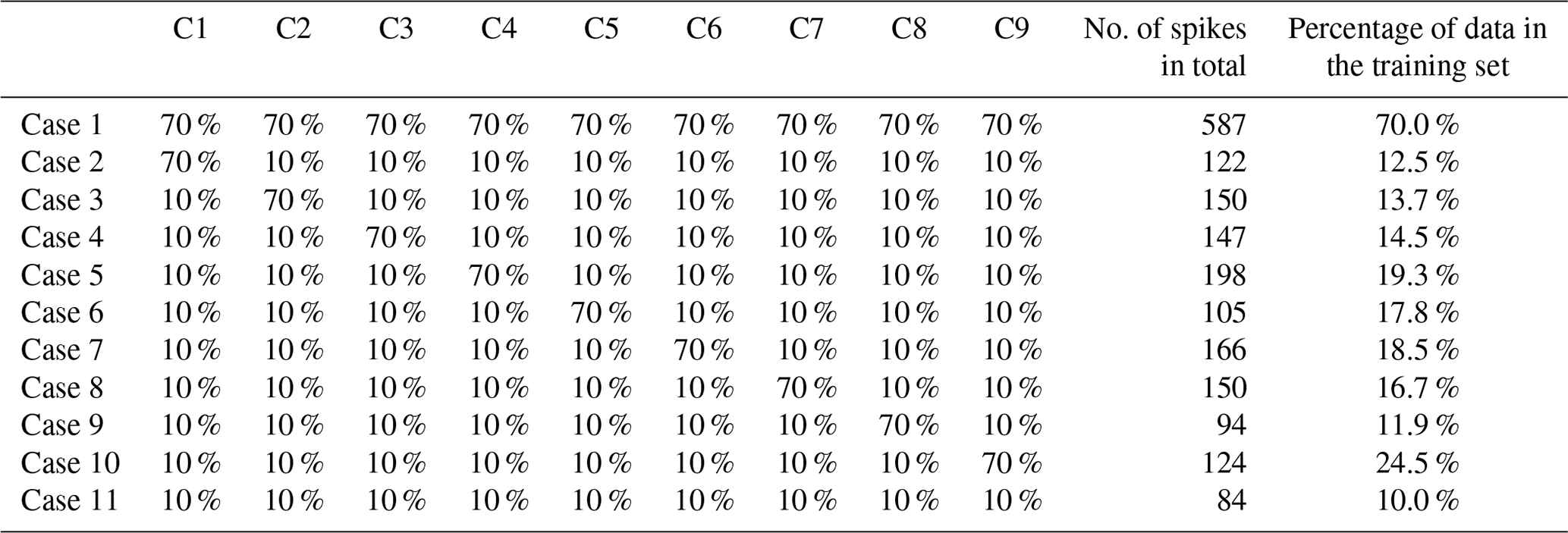
The clusters of spikes were defined using the ward distance to determine a matrix measuring the degree of similarity between spikes using dynamic time warping (DTW) (Sakoe and Chiba, 1978) and to construct a dendrogram. A threshold on the dendrogram allowed us to determine nine different clusters from our dataset. For the second step, we defined 11 cases to construct training sets. Cases 1 and 11 correspond to sampling 70 % and 10 % of the data for training, respectively, equally distributed across the clusters. Cases 2 to 10 correspond to preferentially sampling one cluster over the others for training, by selecting 70 % of the spikes in this cluster and 10 % in all others. The purpose of this stratified data selection is to determine the type of spikes that best allows for the reconstruction of the variations of CH₄ when training a model. At this stage we are not interested in the temporal dependency between observations since we train models with instant values. On a practical application side, a parsimonious model training strategy will require users to expose their sensors to a specific type of “highly influential” spikes on a shorter period from, e.g., a laboratory experiment like the one described above, then train the models upon those spikes and apply them to data collected in the field.

2.5 Assessing aging effects of the sensors

To assess the effect of aging sensors on the reconstruction of CH₄, we conducted a 33 d experiment from 11 August to 12 September 2020, 6 months after the first experiment described in Sect. 2.1.2. The spike generation system was the same. Between the two experiments, the chambers containing TGS sensors had been measuring ambient air pumped from our laboratory roof. To assess the aging effect on the TGS sensors during the 6-month interval, we selected the two models that gave the highest performance for the first experiment and applied them to simulate the spikes generated during the second experiment.

2.6 Finding generalized models that can be used for other sensors of the same type

We were interested in understanding to what extent a model trained with the outputs of a given TGS sensor type in a given chamber could be applied to other sensors of the same type in other chambers. The experiment consisted of training a model per sensor and chamber with the best configuration subset based on the cluster classification outlined in Sect. 2.4. The trained model is then used to reconstruct the CH₄ spikes using data from the TGS in other chambers and compare their performances. For this, we used data from chambers A, C, F and G to train chamber-specific models and used each chamber-specific model to reconstruct CH₄ spikes using data from other chambers, as shown in Table 1. The four chambers have a load resistor of 50 kΩ and contain three TGS sensors each. We did not use data from chambers D and E because they have a load resistor of 5 kΩ, and chamber E contains two of each TGS sensor.

2.7 Metrics for performance evaluation

The performance of the models to reconstruct the dry CH₄ concentrations observed by the CRDS instrument using TGS sensors was assessed using a decomposition of the mean squared deviation (MSD) of the misfits between reconstructed and true CH₄ (Kobayashi and Salam, 2000), to separate the main source of errors when comparing different models. MSD was decomposed into the sum of the square bias (SB), the difference in the magnitude fluctuation (SDSD) and the lack of positive correlation weighted by the standard deviation (LCS). A large SDSD indicates an incorrect reconstruction of CH₄ spike magnitudes. A large LCS indicates an incorrect reconstruction of spike phase or shape. The equations for each error term according to Kobayashi and Salam (2000) are given by

$$\begin{array}{}\text{(5)}& {\displaystyle }\text{SB}={\left(\stackrel{\mathrm{‾}}{{\widehat{y}}_{{\mathrm{CH}}_{\mathrm{4}}}}-\stackrel{\mathrm{‾}}{y_{{\mathrm{CH}}_{\mathrm{4}}}}\right)}^{\mathrm{2}}\text{(6)}& {\displaystyle }\text{SDSD}={\left({\mathit{\sigma }}_{\mathrm{Model}}-{\mathit{\sigma }}_{\mathrm{Ref}}\right)}^{\mathrm{2}}\text{(7)}& {\displaystyle }\text{LCS}=\mathrm{2}{\mathit{\sigma }}_{\mathrm{Model}}{\mathit{\sigma }}_{\mathrm{Ref}}(\mathrm{1}-\mathit{\rho })\text{(8)}& {\displaystyle }\text{MSD}=\text{SB}+\text{SDSD}+\text{LCS},\end{array}$$

where $\stackrel{\mathrm{‾}}{{\widehat{y}}_{{\mathrm{CH}}_{\mathrm{4}}}}$ is the mean of the prediction, $\stackrel{\mathrm{‾}}{y_{{\mathrm{CH}}_{\mathrm{4}}}}$ the mean of the reference observations, σ_Model the standard deviation of the modeled CH₄ time series, σ_Ref the standard deviation of the reference one and ρ their correlation coefficient. All results presented below are using metrics computed for the test set only.

3 Results

3.1 Data preprocessing and baseline correction

Figure 2 shows the preprocessing steps of the dataset, with the identification and removal of the background signal from the spikes in the time series. We removed outliers and the first 30 min of observations in the case of a reboot of the data loggers of each chamber, i.e., during stabilization of the sensors. The original observations on a time step of 2 s were resampled to means of 5 s.

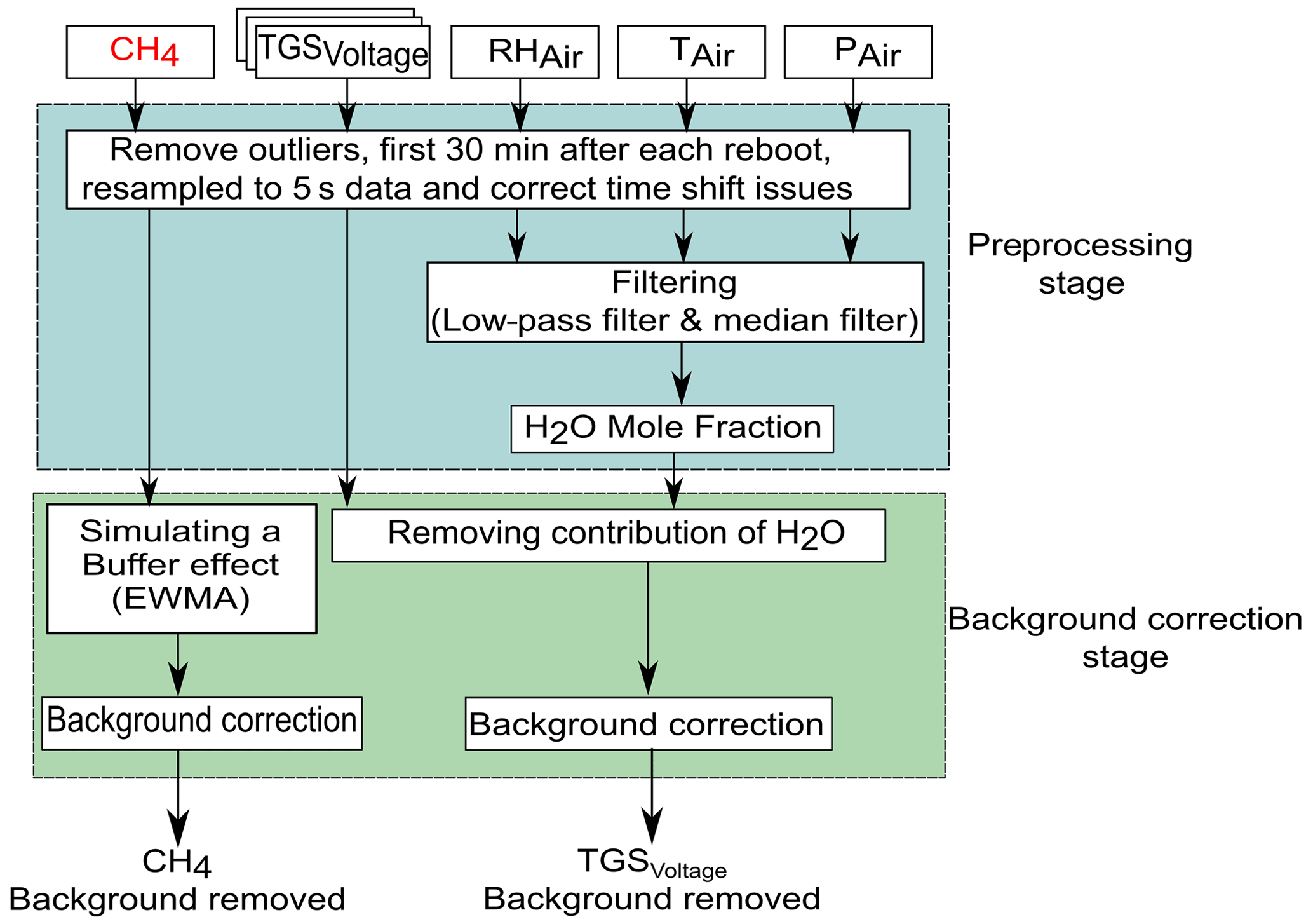
Figure 2 Data preprocessing diagram, correction of H₂O effects, and separation of the spikes from background data in the time series.

Environmental variables (H₂O, temperature and pressure) were filtered using a low-pass filter (Press and Teukolsky, 1990) to remove high-frequency noise from the sensors and circuit connections. The water vapor mole fraction was calculated with Rankine's formula (Eq. 9) from relative humidity (RH; in %) and temperature (T; in ^∘C) from the DHT22 sensors and pressure (P; in Pa) from the BMP180 sensors in each chamber, according to

$$\begin{array}{}\text{(9)}& {\mathrm{H}}_{\mathrm{2}}{\mathrm{O}}_{\mathrm{Mole}\mathrm{Fraction}}=\mathrm{100}\times \left({\displaystyle \frac{\frac{\text{RH}}{\mathrm{100}}\times e^{\frac{\mathrm{13.7}-\mathrm{5120}}{T+\mathrm{273.15}}}}{\frac{P}{\mathrm{100}\mathrm{000}}-\frac{\text{RH}}{\mathrm{100}}\times e^{\frac{\mathrm{13.7}-\mathrm{5120}}{T+\mathrm{273.15}}}}}\right).\end{array}$$

An example of several spikes obtained after the preprocessing and background signal removal is shown in Fig. 3 (see also Fig. A3). The entire spike dataset contains 838 spikes, representing 1.6 % (35 536 5 s observations) of the full dataset.

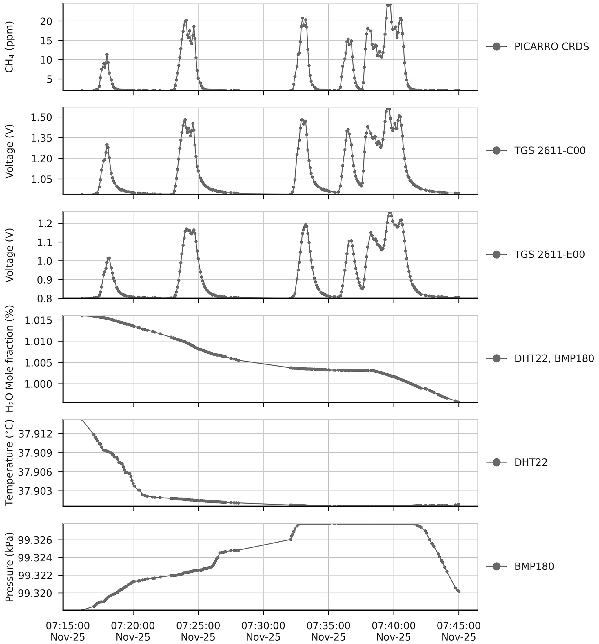
Figure 3 Top to bottom: time series of reference CH₄ signal from CRDS, voltage from TGS sensors, H₂O, temperature and pressure during a period of 30 min, after removing the variations of background signals from the time series and applying the H₂O correction to the voltage signal of TGS sensors. Dots in panels represent actual observations, and lines between dots are drawn to show the shape of the signals.

3.2 Reconstruction of CH₄ spikes

Figure 4 shows the reconstruction of several spikes by the linear, polynomial, random forest (RF), random forest hybrid (RFH) and MLP models using data from the type-C TGS sensor in chamber A. Figure 5 shows the reconstruction results using data from the type-E TGS sensor in chamber A. In both figures, the model training set contains 70 % of the total observations available. The spikes reconstructed by the different models show good agreement with the reference CH₄ signal for the type-C sensors but not for type-E ones which are associated with phase errors and greater noise in the reconstructed CH₄. This behavior can be linked to the carbon filter included on top of the sensing material the of type-E sensor that produces an airflow resistance, leading to a slower response. The linear, RF and RFH models broadly capture the mean amplitude of spikes, but they are less capable of reconstructing small CH₄ variations on the top of the spikes. The RF and RFH models (the latter with a polynomial model) provided very similar outputs, with a small enhancement of the amplitude for RFH during some spikes and noise, especially with type-E sensors (Fig. 5). The MLP model showed a constant underestimation of the spike magnitudes and produced smoother spike shapes, presenting a low-pass filter behavior. The polynomial fit models appeared to perform better. Despite the phase misfit of models with type-E sensors, for all the models, both type C and type E meet our requirement target of an RMSE ≤2 ppm (MSD ≤4 ppm²). With a stricter requirement of an error of less than 5 % of the maximum amplitude of the peaks (RMSE ≤1 ppm), only type C is adequate.

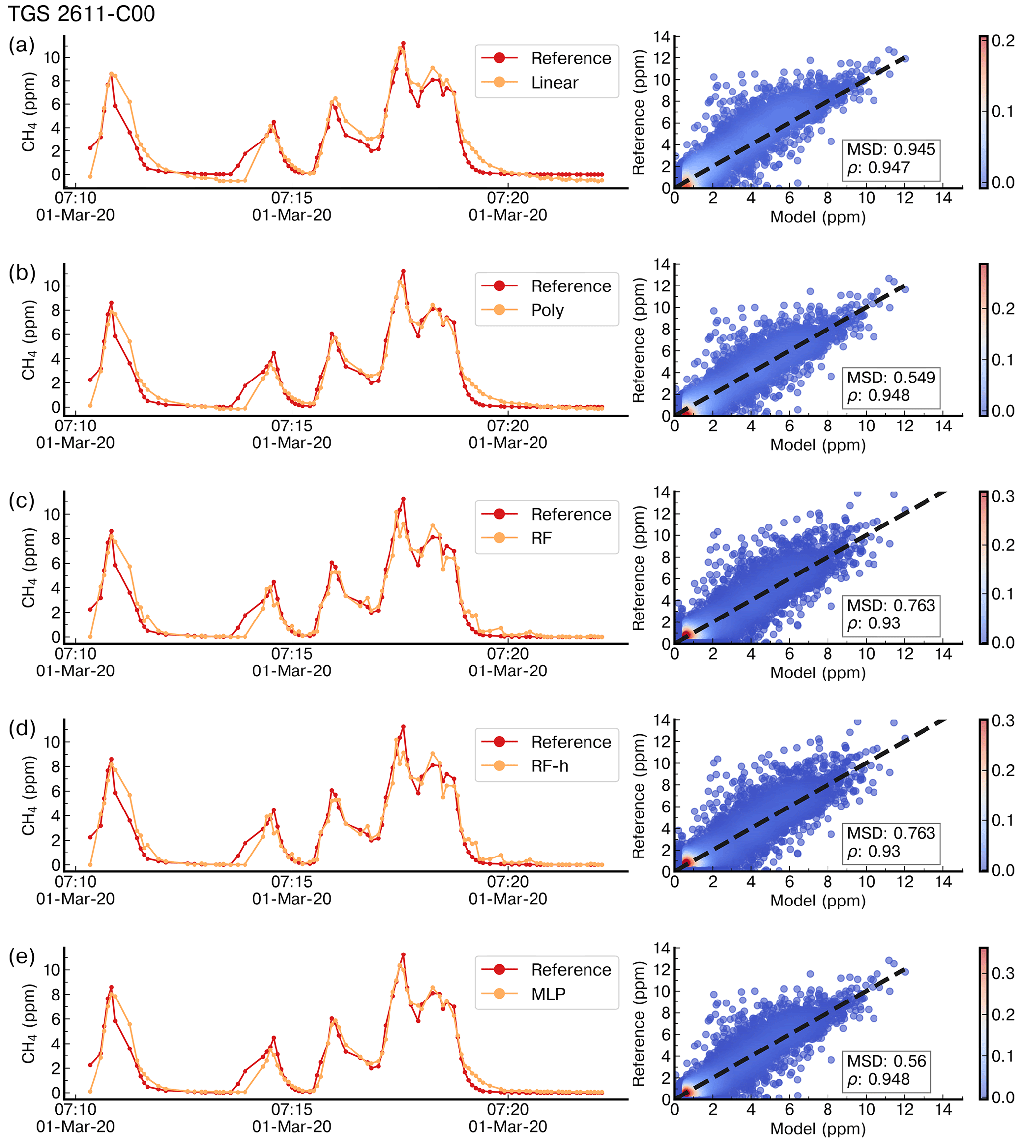
Figure 4 Example of reconstruction of the CRDS reference CH₄ signal on a time step of 5 s for a few spikes in the test set by (a) a linear model, (b) a polynomial model, (c) a random forest model, (d) a random forest hybrid model and (e) a multilayer perceptron model trained with 70 % of data and using as input data from the TGS 2611-C00 sensors only. The right panels show scatter plots between the reference CH₄ signal and the modeled outputs. The color code is the density of observations.

Figure 5 Same as Fig. 4 but for data from the TGS 2611-E00 sensors only.

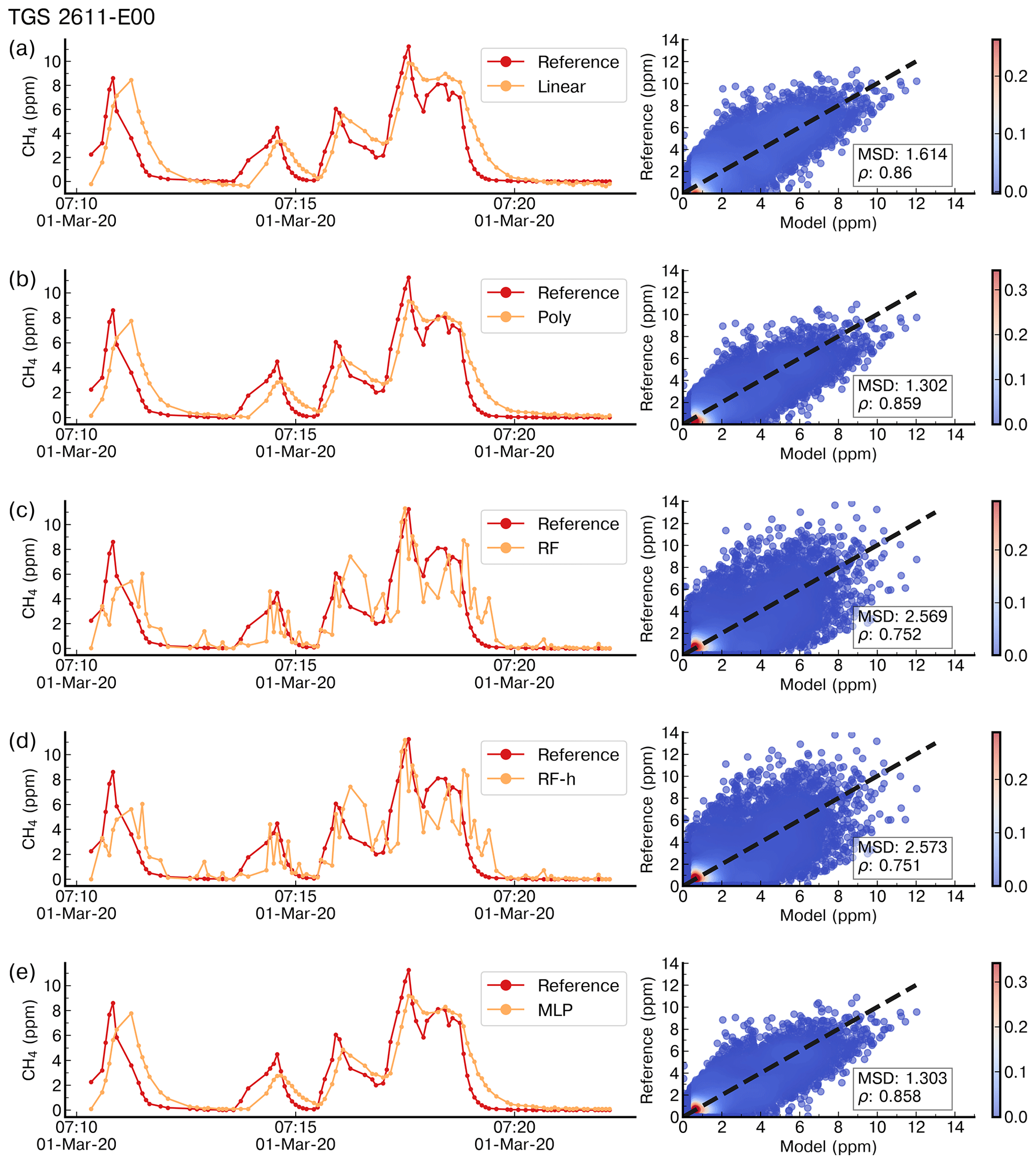
Figure 6 shows the distributions of the correlations (ρ) between modeled and observed CH₄ spikes for the 20-fold validation periods (test sets) for different models. We distinguished two groups of models, based on median values of ρ. The first group corresponds to models trained with type-E sensor data only, characterized by ρ_Median≤0.93. The second group corresponds to models trained with type-C sensor data only or with data from both types of sensors, characterized by a higher ρ_Median≥0.96. Among the models in the first group, the polynomial model gave the largest correlations (ρ_Median=0.92, interquartile range (IQ) =0.035 and 0.013 for a test set size of 30 % and 50 % respectively). Among the models in the second group, the polynomial model also showed the largest correlation, especially with both types of sensors, and a training set of 50 % of the observations (ρ_Median=0.98, IQ =0.006), closely followed by the MLP model with the same inputs and the same training set size (ρ_Median=0.98, IQ range =0.006). The random forest, random forest hybrid and MLP models also showed high correlations when input data are from the type-C sensors, and the training uses 70 % of the observations (RF ρ_Median=0.973, RFH ρ_Median=0.973 and MLP ρ_Median=0.982). These three models however had lower correlations when input data are from type-E sensors (RF ρ_Median=0.897, RFH ρ_Median=0.898 and MLP ρ_Median=0.925). Phase errors were reduced when training the models with either type-C sensor data or data from both sensors. The length of the training set had an important impact on the spread of the correlations across the 20-fold periods. With 70 % of observations in the training set, the IQ of the correlations increased, whereas for a smaller training set, the IQ was smaller, but the distribution of the correlations showed more outliers. The inclusion of environmental variables (Fig. 6b) as input to models, in addition to voltages from TGS sensors, reduced the phase error in the random forest models significantly but produced little improvement in the results from other models. Summary statistics of the distribution of correlations between the modeled and observed CH₄ spikes are shown in Tables A5 and A6.

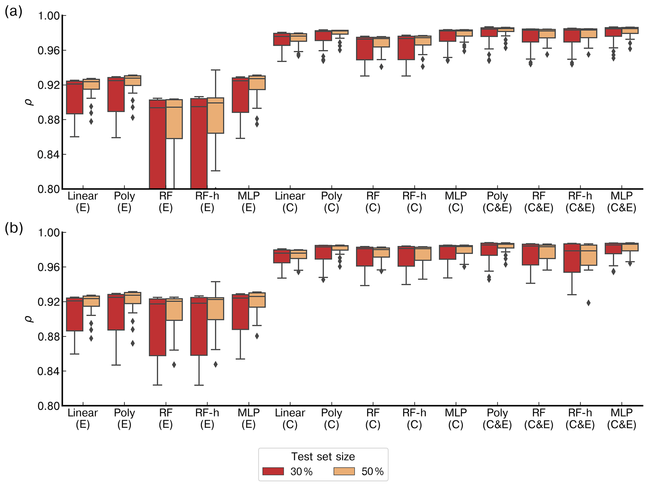
Figure 6 Comparison of the Pearson correlation coefficient (ρ) distributions between models on the test set for a 20-fold cross-validation. The boxes are the interquartile of the distribution of ρ, the whiskers are the 5th and 95th percentiles, and the black line is the median. (a) Models in which the inputs are only voltage from the Figaro^® TGS sensors. (b) Models in which the inputs include voltage from low-cost sensors and environmental variables (H₂O, temperature and pressure). “Linear” represents the linear or multilinear model, “Poly” the polynomial model, “RF” the random forest model, “RF-h” the random forest hybridized with a polynomial regression and “MLP” the multilayer perceptron. Below each model, labels denote which TGS sensor was used: “C” is the TGS 2611-C00, “E” the TGS 2611-E00 and “C & E” both sensors at the same time. The red box plots represent the results of models with a test set size of 30 % of the total observations and the yellow ones a test set size of 50 %. Note that the y axis was limited in a range to distinguish the different models.

Figure 7 shows the MSD error decomposition for the different models and for the two training set sizes of 70 % and 50 %, respectively. We observed that the LCS component of the MSD (related to a phase misfit of the modeled series) is the principal source of error across the different models, regardless of the input used or the size of the training set, meaning that models have more difficulties to reproduce the phase of the spikes than their amplitude. A systematically higher LCS error was obtained when data from type-E sensors are used as input, and there is also a larger SDSD error with this type of sensor. For example, the largest LCS error was found with a training set of 70 % for the random forest models (LCS_RF=4.67 ppm², LCS_RF=1.24 ppm² and LCS_RF=0.79 ppm² with type-E sensor data, type-C sensor data and both types respectively) as well as for the RFH models, when compared with other models. Additionally, the inclusion of environmental variables had little effect on the model performance. This was clearly shown for the LCS error of the polynomial model, for a training set of 70 % of the data, which was identical with and without environmental variables as input (LCS_poly=3.0 ppm² for the type-E sensor, LCS_poly=0.84 ppm² for the type-C sensor and LCS_poly=0.7 ppm² for both types). Reducing the size of the training set mostly affected the SDSD component, by slightly lowering the capability of models to reconstruct the amplitude of the CH₄ spikes. For the non-parametric models, reducing the size of the training set also increased the bias error (SB), an effect that was partially mitigated with the inclusion of environmental variables. Amongst the non-parametric models, the MLP obtained a similar performance to the parametric polynomial model (MSD_MLP=3.2 ppm², MSD_MLP=0.85 ppm² and MSD_MLP=0.7 ppm² for type-E sensors, type-C sensors and both types together, respectively). To summarize, the choice of the sensor type used to train the models affected the reconstruction error more than the selection of the model. The type-C sensor data produced the lowest error compared to type-E, irrespective of the model used. Overall, the polynomial model gave a better performance than the non-parametric models. More detailed statistics are summarized in Tables A1 and A2.

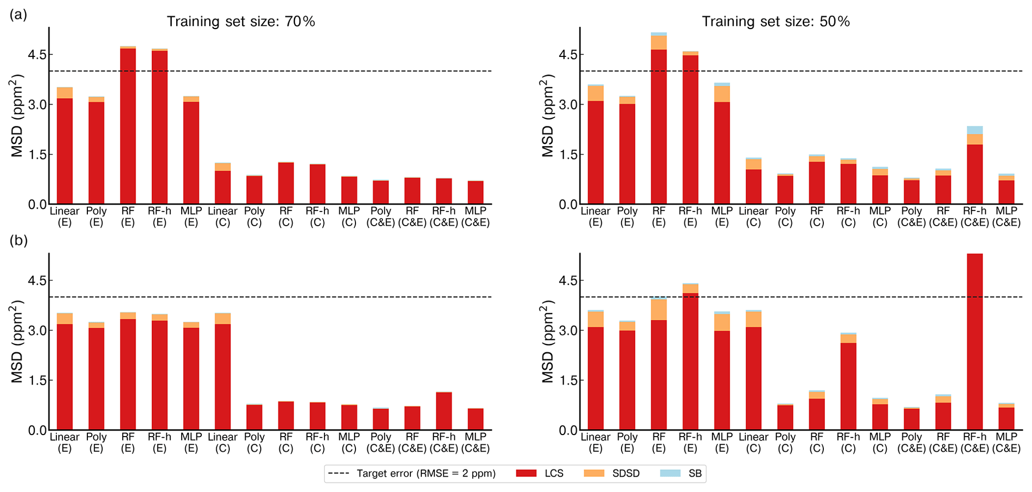
Figure 7 Comparison of the mean standard deviation (MSD) across the different models on the test set for a 20-fold cross-validation. (a) Models with only voltage of TGS sensors as input. (b) Models including environmental variables and voltage of TGS sensors as input. Left panels show the performances on a training set size of 70 % and right panels a training set size of 50 % of the total observations. The stacked bars show the contribution of each component of the MSD to the total error. The lack of positive correlation weighted by σ (LCS) is shown in red, the difference in the magnitude fluctuation (SDSD) in orange and the simulation bias (SB) in green. Notation for the models is the same as for Fig. 6.

3.3 Results of parsimonious training tests

Figure 8 shows the result of the spike clustering. Based on spike similarity, we found nine clusters. The peaks with short durations (under 50 s) and containing only one spike were grouped into cluster C1 (signal amplitude (sa) ≤6 ppm) and cluster C3 (6 ppm ≤ sa ≤12 ppm). Peaks with longer duration (over 50 s) were grouped into clusters C2 (sa ≤4 ppm) and C4 (4 ppm ≤ sa ≤8 ppm). Peaks with very long duration (between 50 s to 1.5 min) were grouped into cluster C5. Peaks with a small concentration at the beginning (around 6 ppm) followed by a larger peak (up to 12 ppm) were grouped into cluster C6. Peaks with larger concentrations (≥12 ppm) and complex in shape were grouped into clusters C7, C8 and C9, respectively. The cluster regrouping the largest number of spikes (191) was C4, and the one with the smallest number of spikes (17) is C8.

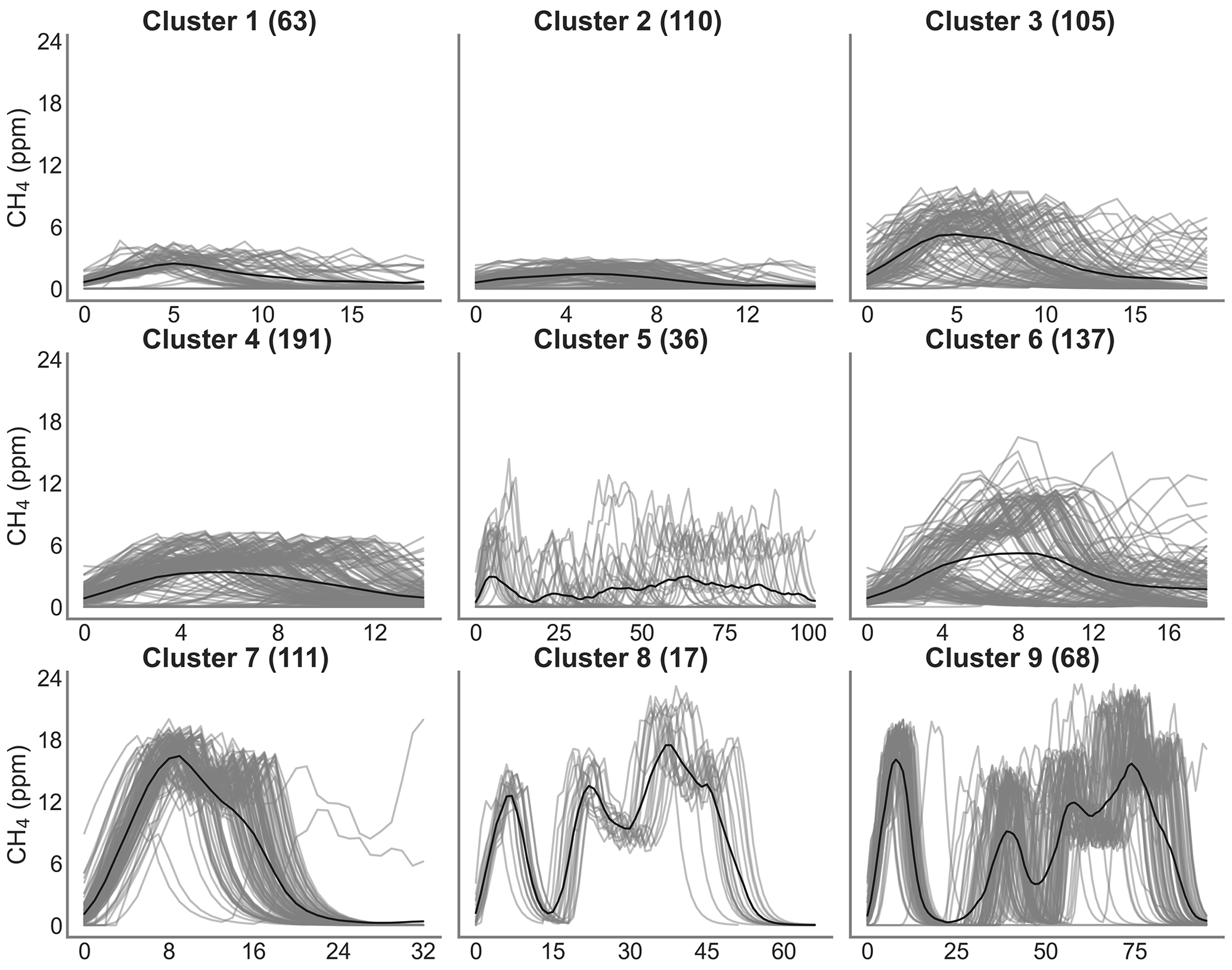
Figure 8 Clustering of peaks using DTW on the reference instrument. On the title of each plot, the number inside the parentheses corresponds to the number of spikes attributed to each cluster. Thin gray lines represent all the peaks inside each cluster, and the black line is the mean of all the peaks corresponding to each class.

Figure 9 shows the error of the models against the test set, for each of the training cases listed in Table 2, based on spikes chosen from different clusters for doing the training (see Sect. 2.4). The results are summarized in Tables A3 and A4. First, the polynomial and MLP models performed consistently better than the other models, the MLP being slightly better for most of the cases. In contrast, the linear, random forest and random forest hybrid models had the highest error, regardless of the sensor type or the addition of environmental variables. To compare the performances of the models trained by spikes from different clusters (Table 2), we ranked them by their error. The MLP model was used with type-C sensor data as input, and training with spikes from Case 10 (124 spikes) produced the smallest error (MSD =0.79 ppm²), followed by the same model for Case 8 (MSD =0.85 ppm², 150 spikes), Case 9 (MSD =0.86 ppm², 94 spikes) and Case 11 (MSD =0.87 ppm², 84 spikes). For the MLP model, Case 4 (147 spikes), Case 1 (587 spikes) and Case 7 (166 spikes) performed slightly worse, with a MSD =0.89 ppm². Finally, Case 2 (MSD =0.9 ppm², 122 spikes), Case 3 (MSD =0.91 ppm², 150 spikes), Case 6 (MSD =0.93 ppm², 105 spikes) and Case 5 (MSD =0.95 ppm², 198 spikes) showed worse performances. From the model ranking, we derived the following conclusions. Firstly, the smallest error did not correspond to the most parsimonious training set (Case 11) but to a larger training set (Case 10, 25 % of the data). Nevertheless, we found that Case 11, which was constructed with an even selection of spikes from all the clusters, each in a modest proportion (10 % from each cluster), provided better performance than most of the other training cases. This result shows that some clusters introduce less information or have redundancy. Overall, the best performances corresponded to Cases 10, 8 and 9, which all included spikes with complex shapes from clusters C7, C8 and C9. Training models with a sample of those spikes thus ensured better model performances.

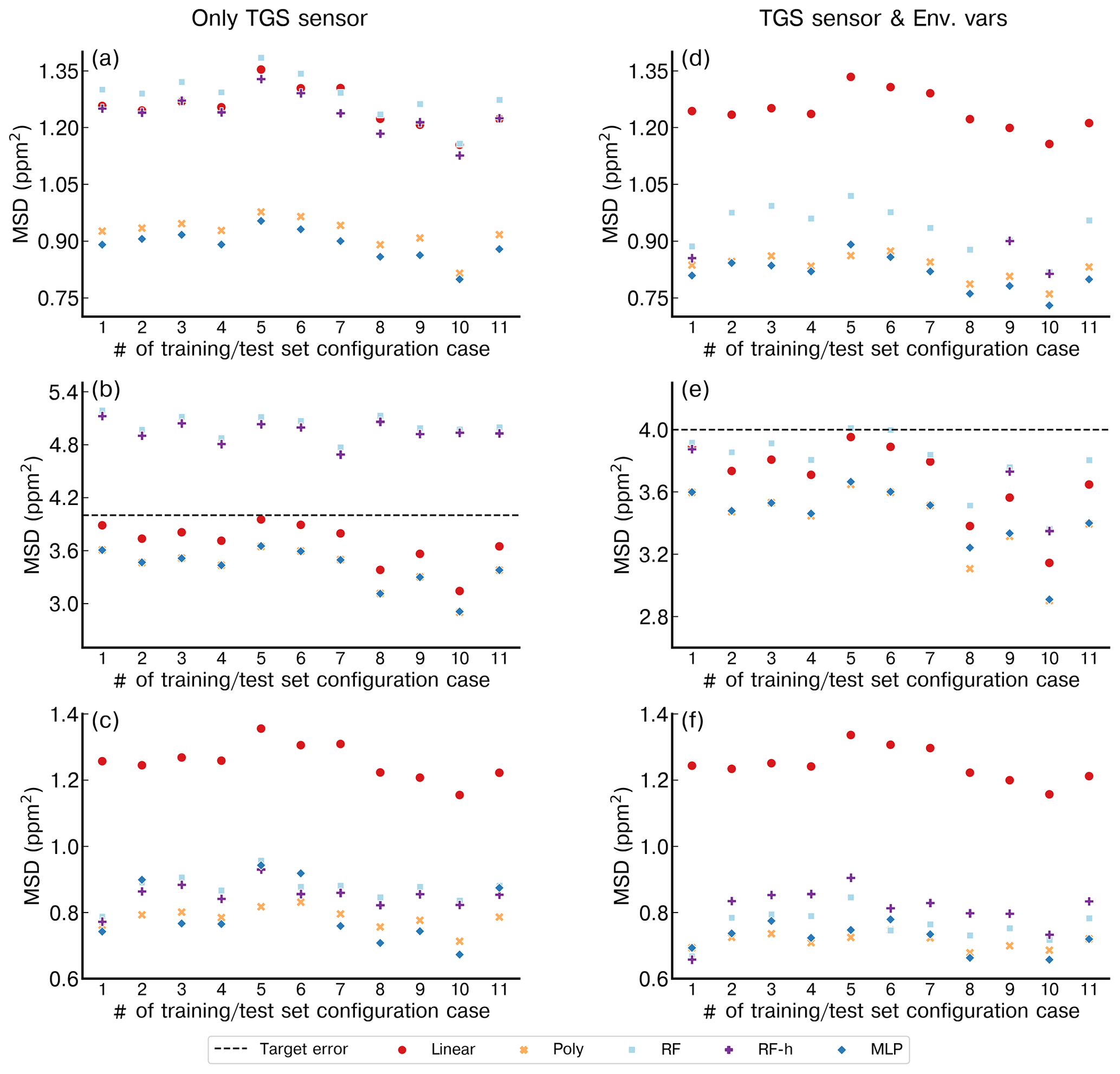
Figure 9 Performance of each model for the different configurations of training and test set (1 to 11 in the x axis) considering the identified clusters. (a) Only Figaro^® TGS 2611-C00 data as input. (b) Only TGS 2611-E00 data as input. (c) Data with both Figaro^® sensors as input. (d) TGS 2611-C00 data and environmental variables. (e) TGS 2611-E00 and environmental variables. (f) Both TGS sensors and environmental variables. Note the different y axis for panels (b) and (e).

3.4 Results for possible aging effect on model performance

To test for a possible aging effect of the sensors, we selected the two best models (polynomial regression and MLP) found in the previous section and trained them following the best training configuration (Case 10). After being trained using data from the first experiment, these two models were applied to reconstruct the spikes of the second experiment, 6 months later. A summary of the results is presented in Table 3. We observed that after 6 months, the RMSE had increased in a range between 0.57 to 0.85 ppm between both experiments. The models trained with type-E sensor data showed a smaller degradation (higher RMSE) after 6 months compared to those trained with the type-C sensor data. Considering the amplitude of the peaks that we aim to reconstruct (∼24 ppm), a possible drift caused by aging effects on the sensors appeared to be a small source of error in the reconstruction of CH₄ spikes during the second experiment. Assuming that the error of the sensors increased linearly with time, we determined an error “drift rate” by computing the ratio of the difference in the error from both experiments divided by the time between them. We observed that for all the cases, the difference in the error is less than 1 ppm after 6 months and the mean RMSE on the second experiment is less than 2 ppm in all cases, except for the models trained with only the type-E sensor. Thus, even with aging, the type-E sensors would still meet our requirement of a RMSE smaller than 2 ppm. This shows the capability of our models to reconstruct spikes despite possible aging effects of the sensors.

Table 3 Comparison of error for reconstructing spikes in experiment 2, using the two best models (polynomial and MLP) trained with the best training set configuration during experiment 1.

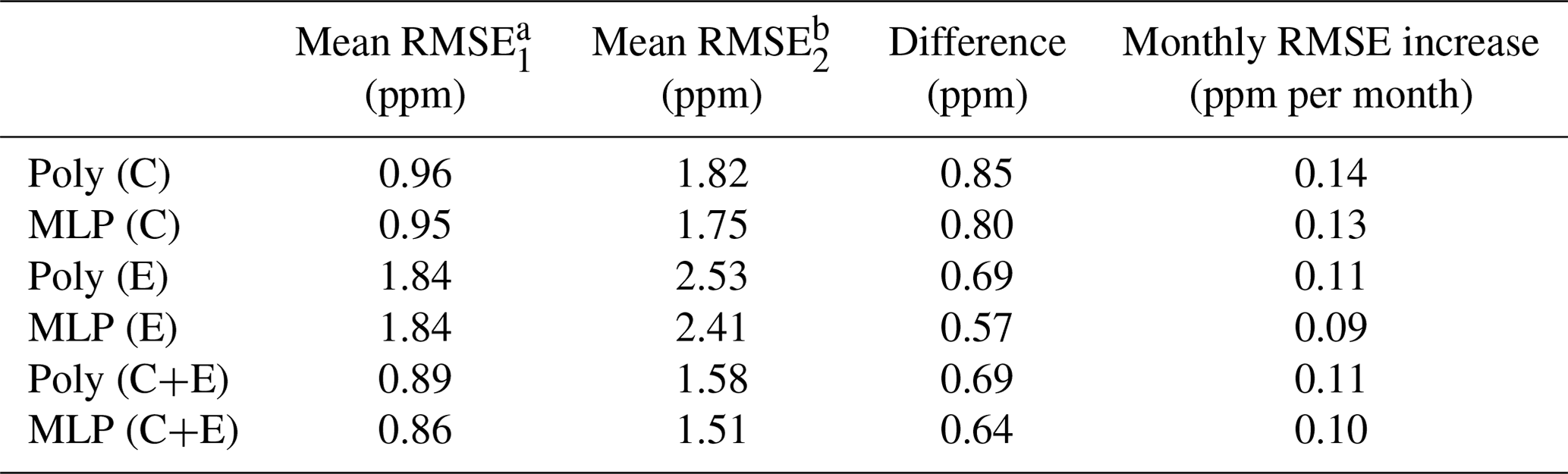
^a For spikes reconstructed during experiment 1.
^b For spikes of experiment 2 reconstructed with models trained on experiment 1.

3.5 Generalized models

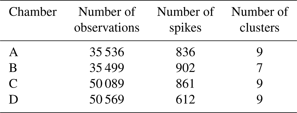
In this section, we address the comparison of model performances when we train a model on a subset of the sensor data from one chamber and reconstruct the spikes of the other chambers. Table 4 presents a summary of the number of spikes, observations and clusters analyzed for each chamber. The number of clusters, as well the number of spikes, was not equally captured by all the chambers. Only three chambers, A, C and D, shared the same number of clusters. Chamber B had a more limited number of peaks due to a reduced sampling period.

Table 4 Summary of spikes, observations and clusters detected following the procedure explained in Sect. 2.4 for chambers A, B, C and D.

To illustrate the performance of models for their ability to be generalized from one chamber to another, we selected the polynomial model with input data from the type-C sensor (Fig. 10) and from the type-E sensor (Fig. 11). The same results with the MLP model are shown in Figs. A7 and A8, respectively. The data in Fig. 10 indicate that the error was lower for the test set of the chamber on which the model was trained than for the test sets of other chambers, as expected. In Fig. 10a, c and d, we observed that the models trained with the data from chambers A, C or D produced good performances for reconstructing the spikes of another chamber and met the requirement target of an RMSE ≤2 ppm. The models trained with the data from chamber B (Fig. 10b), however, performed poorly in reconstructing the spikes from the other chambers and met the target requirement only when trained using data from the same chamber. The performances of the MLP model were similar to those of the polynomial model in terms of generalization from one chamber to another. When trained by data from the type-E sensor, our models were found to be less transferable from one chamber to another, meaning they had a larger error for the test sets of another chamber than for the one used for training (Fig. 11). We inferred that the reconstruction of spikes from models of other chambers needs to be coherent with the number of clusters of the chamber used for training in order to ensure transferability of the models. This is the case for chambers A, C and D for which nine clusters were detected and the distribution of peaks within the clusters was similar (Figs. 8, A9 and A10). On the other hand, if the clusters are not similar between chambers, the transferability of models is lower.

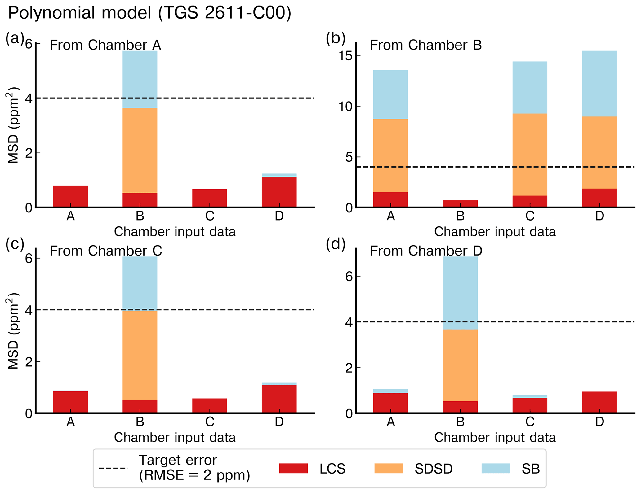
Figure 10 Reconstruction error of the peaks for the polynomial model with TGS 2611-C00 as input using the best stratified training case from (a) chamber A, (b) chamber B, (c) chamber C and (d) chamber D to reconstruct the peaks from the other chambers (listed on the x axis) with data from the same type of sensor. Note the different ranges of the y axis for the panels (b) and (c).

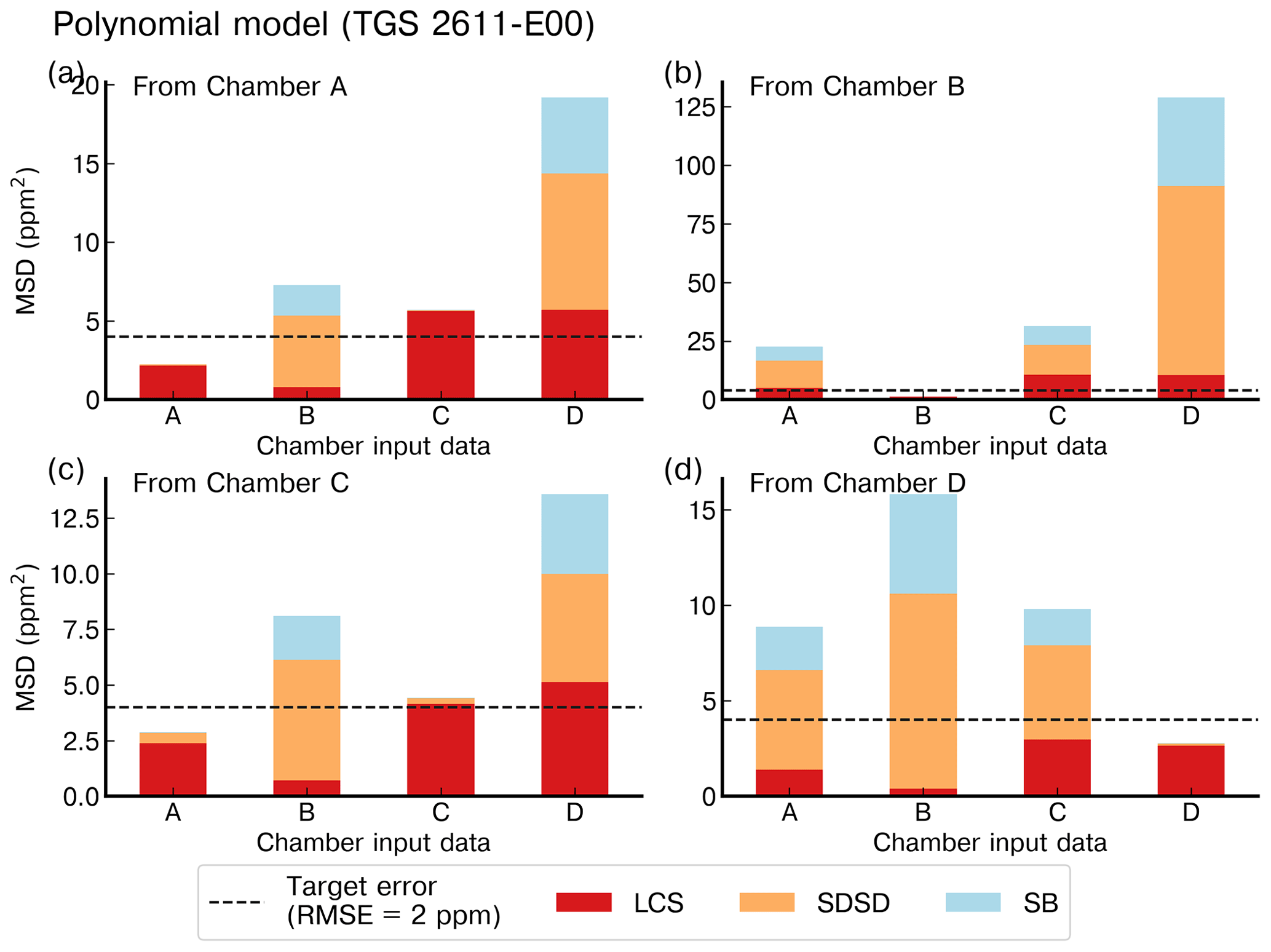
Figure 11 Reconstruction error of the peaks for the polynomial model with TGS 2611-E00 as input using the best stratified training case on (a) chamber A, (b) chamber B, (c) chamber C and (d) chamber D to reconstruct the peaks from the other chambers with data from the same type of sensor. Note the different ranges of the y axis.

4 Discussion

Our results show that a preprocessing of the data to remove H₂O effects and separate spikes from ambient air CH₄ variations, followed by a careful definition of the training set, provides capabilities for different models to reconstruct the CH₄ spikes on a 5 s time step, across a large range of concentration variations and spike durations, meeting our requirement of a target error of RMSE ≤2 ppm. The TGS 2611-E00 (type E) was the sensor with the poorest performance, regardless of the model employed or of the subset of data used to train models, as shown by our tests with five chambers, each containing five different sensors. The model performances for TGS 2611-E00 were thus always poorer than for TGS 2611-C00 (type C), with a degradation in the reconstruction coming from the larger misfit of the phase of the spikes signal than with the TGS 2611-E00 sensors. This probably is related to the carbon filter that is integrated within this type of sensor to improve the selectivity. An additional step of the preprocessing algorithm could help to correct problems due to the carbon filter. The MSD error decomposition showed that the sources of error in the reconstruction were mainly from an inaccurate reconstruction of the phase, followed by a misfit of the magnitude of the spikes. Models have produced a reasonable estimation of the magnitude, which is important from a policy perspective, since information of the magnitude can be of value when monitoring emission magnitudes despite the errors in reconstructing the phase of the peaks. The inclusion of environmental variables reduced the LCS component of the MSD, especially for non-parametric models. Nevertheless, for the type-E sensor, adding environmental variables increased the error in the reconstruction of the magnitude. The presence of other electron donors, such as ethane and isobutane, also needs to be accounted for in the modeling including as a predictor or in the correction of the baseline. Finally, we found that the error always increased with the reduction of the length of the training set, as previously shown by Rivera Martinez et al. (2021). This sensitivity to the training set mainly affected the non-parametric models due to their limited capability of extrapolation and their requirement of large datasets to keep good performances.

How do our approach and results compare with previous studies?

Malings et al. (2019) performed a comparison of different calibration approaches, including linear, quadratic, Gaussian, clustering, ANN and hybrid random forest models across low-cost sensors measuring different species (CO₂, CO, NO₂, SO₂ and NO) with the aim to calibrate Real-time Affordable Multi-Pollutant monitors (RAMP) to assess the air quality within a city, using a network of sensors. Their set of sensors included an NDIR CO₂ sensor, an Alphasense photoionization detector and an Alphasense electrochemical unit. They found that a quadratic regression and a hybrid RF model produced the best performance across different pollutants for training sets with durations between 21 and 28 d and observations with a resolution of 15 min. Our results showed that the hybrid random forest model did not perform as well as the polynomial model or the MLP for the reconstruction of CH₄ spikes using data from TGS sensors and that these models were sensitive to the length of the training set for the k-fold cross-validation. An improvement of our models' performances could be achieved with a selection of the proportion of observations used for the parametric model. Nevertheless, the polynomial model gave consistently better results regardless of the inclusion of environmental variables.

Casey et al. (2019), Rivera Martinez et al. (2021) and Eugster et al. (2020) used ANN models to derive CH₄ concentration from observations of TGS sensors and obtained good performances. Casey et al. (2019) suggested that the inclusion of correlated species (e.g., CO₂) rather than the type of sensor led to better performance for their MLP model to reconstruct CH₄. The performance of their ANN model to reconstruct CH₄ variations provided an RMSE of 0.13 ppm for a range of variation between 1.5 and 4.5 ppm. Eugster et al. (2020) also found that the inclusion of other driving variables could increase the performance of ANN models. Their overall model performances for 7 years of continuous CH₄ monitoring on ambient air in northern Alaska (range of variation between 1.7 and 2.1 ppm) with a Figaro^® TGS2600 gave an RMSE of the residuals of 0.043 µmol mol⁻¹. Our results showed that different types of TGS sensors used with the same model gave complementary information by reducing the error of the reconstruction and should be used, especially with non-parametric models. The performance of our best model for CH₄ spikes with concentrations much larger than those measured by Eugster et al. (2020), produced under controlled laboratory conditions, provides a mean RMSE of 0.9 ppm for a range of CH₄ variation between 3 and 24 ppm, which were thus rather comparable results. Regarding the calibration strategy, the clustering approach allowed us to determine nine clusters of spikes in our dataset, with three of them regrouping the largest peaks with complex shapes. This classification allowed us to understand the impact of each cluster in the training. Cluster 9, composed of peaks of complex shape and with a range of variation between 3 and 24 ppm, was the one that provided the best information for training the models, due to the fact that spikes present on this cluster include information of larger and shorter peaks, medium peaks, and larger peaks with patterns on top of the peaks. With the parsimonious training using Case 10, corresponding to a high proportion of peaks from cluster 9, we were able to reduce the length of the training dataset from 70 % to 25 % while maintaining similar performance. This approach has strong potential to reduce the length of the training set by only selecting observations from specific clusters defined from the data and which represent the entire dataset. This approach is designed with an a priori knowledge of the typical concentrations the sensors will be exposed to. Although, exposing sensors to a wide range of concentrations, like the ones included in cluster 9 from our experiment, can lead to having a large variety of examples for the training of the calibration models.

Concerning the aging effect of the sensors, after 6 months, we observed only small increases in the RMSE of our models, between 0.6 and 0.8 ppm, corresponding to an error increase rate of 0.1 ppm per month. These results show that models would require less calibration in environments with low variations, or invariability, on the clustering structure. But for a deployment on sites with high variability on the clustering structure, periodic re-calibrations would be needed. Our results also showed the capability to transfer the models from one chamber to another, provided that the chamber used for testing contains data with the same range of CH₄ variations as the chamber used for training, which can be assessed by our clustering analysis of the data.

5 Conclusions

We performed a systematic comparison of different parametric and non-parametric models to reconstruct atmospheric CH₄ spikes under laboratory conditions, based on the voltages recorded by low-cost metal oxide sensors. Other environmental variables such as temperature, pressure and water vapor were used. The true CH₄ time series comes from a high-precision instrument run alongside the low-cost sensors. The best models were a second-degree polynomial function and a multilayer perceptron model. These two models both meet our requirements of a RMSE smaller than 2 ppm. We found that the main limitation was the large fraction of data (70 %) needed to train the model. This would limit the use of low-cost sensors in the field, as they would need to be frequently trained with an expensive instrument at the same location. This limitation was partly overcome by adopting a stratified training strategy, namely to perform the training on fewer but more influential spikes selected in orthogonal clusters applied to the whole dataset. This parsimonious training allows us to use only 25 % of the data to keep a model performance compliant with our 2 ppm RMSE threshold. Understanding the number of spikes required for the training of the models can help to define a cost-effective strategy for deployment of the sensors. We also showed that sensors' aging effects after 6 months did not degrade the performances of our models too much. Finally, TGS 2611C-00 was superior to the TGS 2611-E00 model. For this experiment we generated about 800 peaks with some predefined shapes; future implementations should consider increasing the diversity of shapes and durations of the generated peaks. Regarding the models employed, we assessed the performances of models that consider no time dependency in the signal; more complex models that allow us to include the time dependence such as recursive neural networks (RNNs) should be tested.

Appendix A

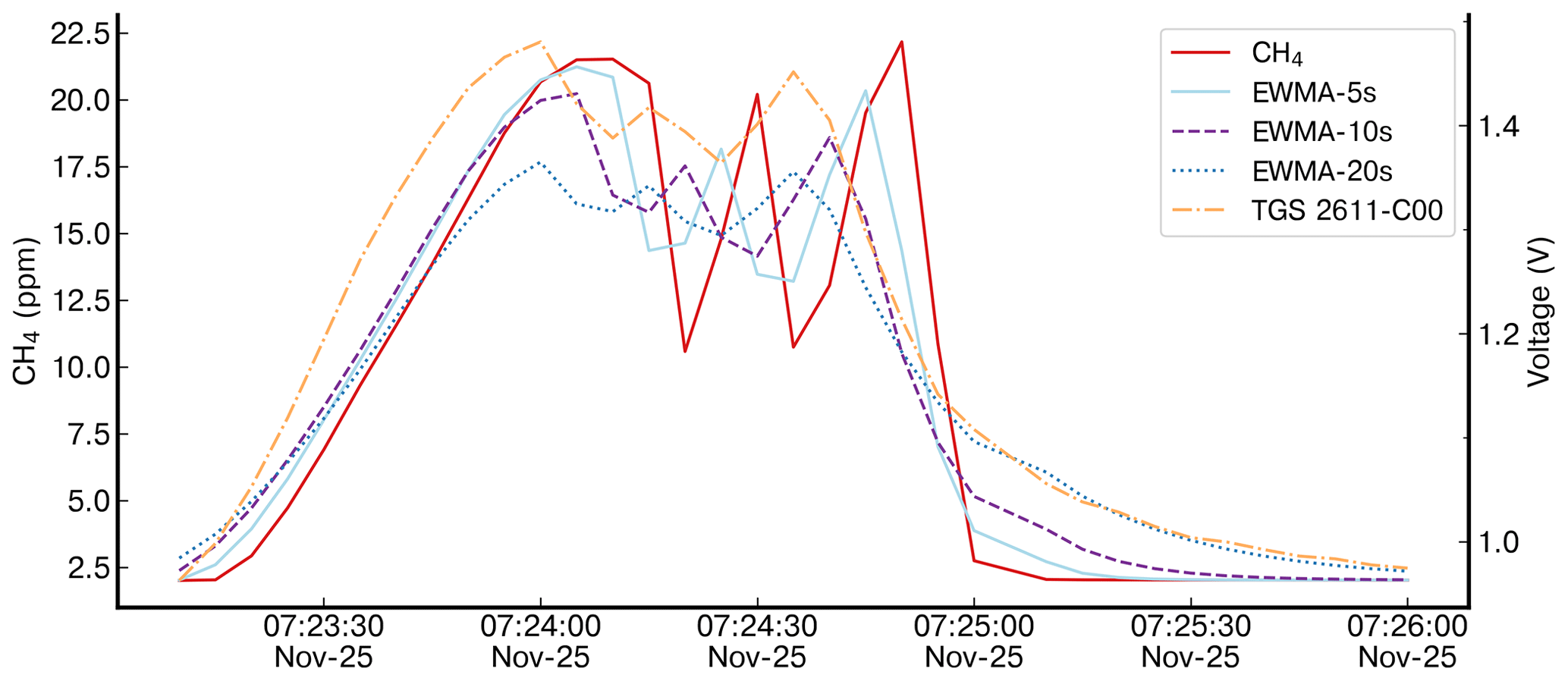
Figure A1 Different time constant values of the exponential weighted moving average (EWMA) applied to the reference instrument. The reference instrument is shown by dotted red lines. The applied smoothing for three values of time constant (5, 10 and 20 s) is denoted “EWMA” for one peak and the TGS 2611-C00 voltage from logger A to compare the smoothing effect shown by the dotted yellow lines.

Figure A2 Derived contribution and correction of water vapor for the Figaro^® TGS 2611-C00. (a) The raw voltage signal (gray) and the derived cross-sensitivities to H₂O (blue). (b) The cross-sensitivity-corrected signal.

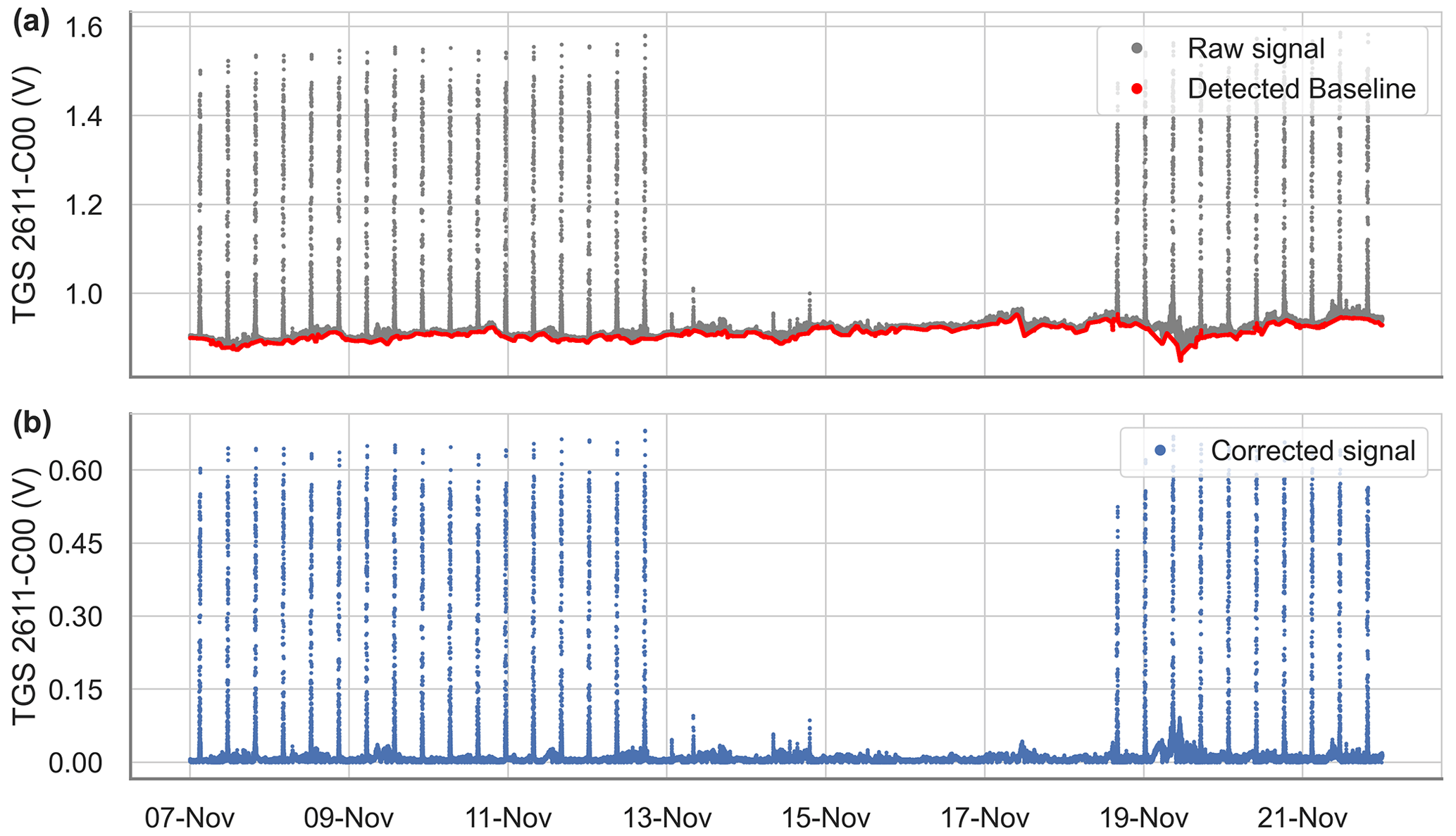
Figure A3 Example of the baseline extraction and correction for the Figaro^® TGS 2611-C00 over 15 d. (a) Raw signal (gray) and detected baseline with the spike detection algorithm (red). (b) Voltage signal with the corrected baseline.

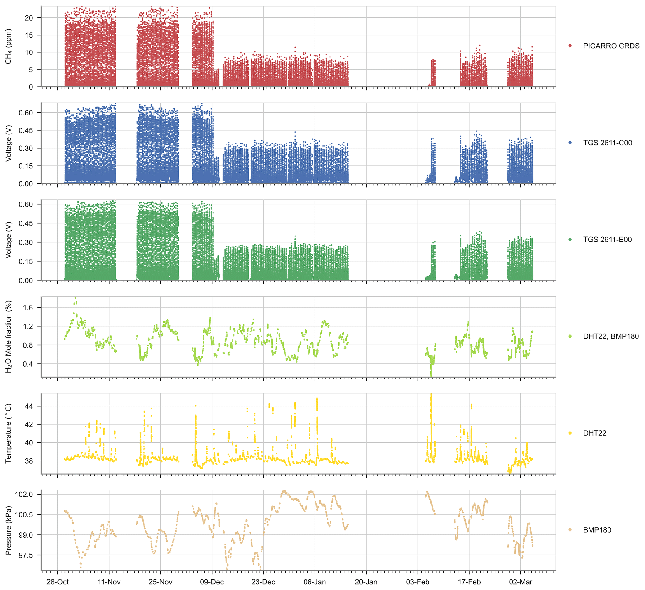
Figure A4 Time series of the reference CH₄ signal, Figaro^® TGS sensor and environmental variables for the entire experiment.

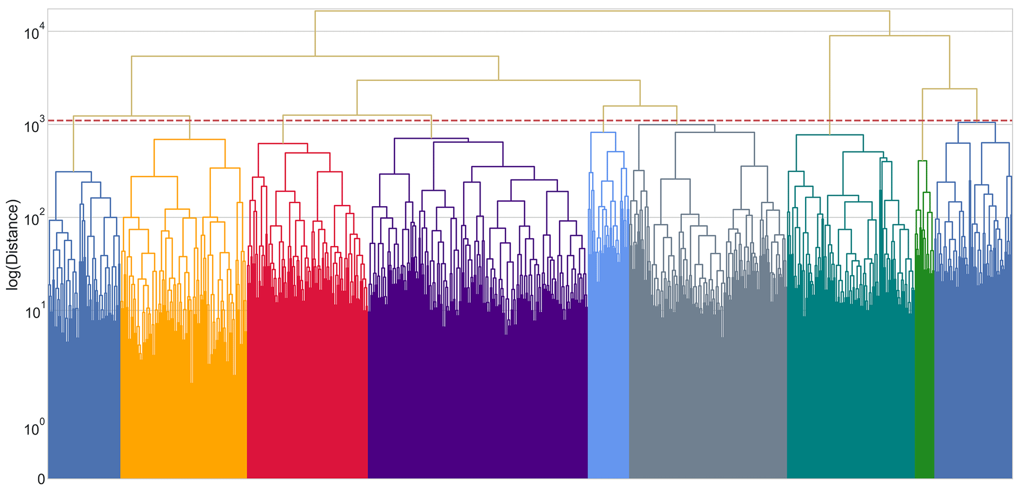
Figure A5 Dendrogram constructed from the distance matrix computed using the DTW metric. The dotted red line represents the threshold used to determine the clusters. Each color under the threshold line represents one cluster of peaks. Note that the y axis was rescaled to the logarithm of the “ward” distance to appreciate the threshold and the clusters better.

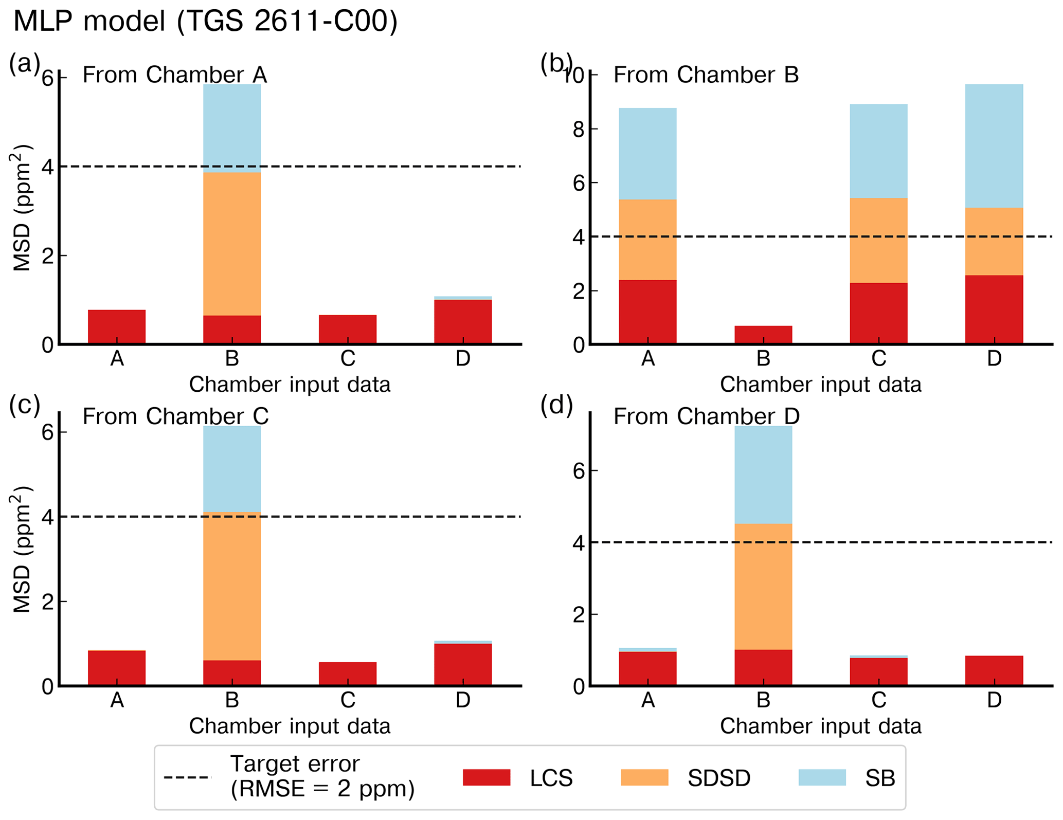
Figure A6 Reconstruction error of the peaks for the MLP model with the TGS 2611-C00 as input and using the best stratified training on (a) chamber A, (b) chamber B, (c) chamber C and (d) chamber D. The first column on each panel is the reconstruction error on the test set of the chamber on which the training was done; the other columns are the reconstruction on the whole dataset for that chamber on the same sensor. Note the different ranges of the y axis.

Figure A7 Reconstruction error of the peaks for the MLP model with the TGS 2611-E00 as input and using the best stratified training on (a) chamber A, (b) chamber B, (c) chamber C and (d) chamber D. The first column on each panel is the reconstruction error on the test set of the chamber on which the training was done; the other columns are the reconstruction on the whole dataset for that chamber on the same sensor. Note the different ranges of the y axis.

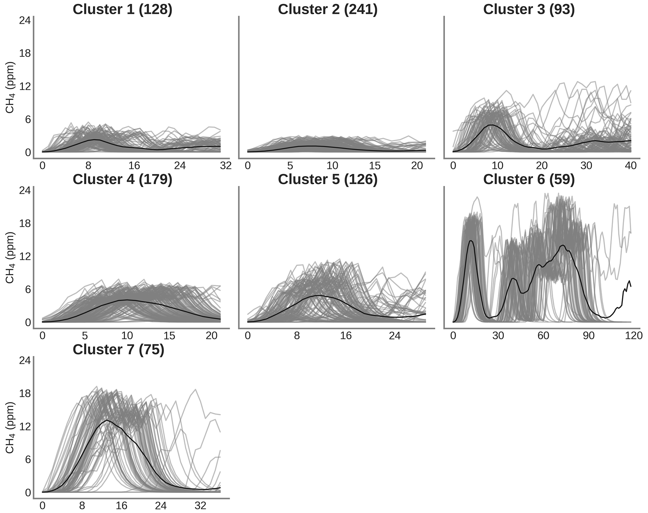
Figure A8 Clustering of peaks using DTW on the reference instrument for the same spikes detected by sensors on chamber B. On the title of each plot, the number inside the parentheses corresponds to the number of spikes attributed to each cluster. Thin gray lines represent all the peaks inside each cluster, and the black line is the mean of all the peaks corresponding to each class.

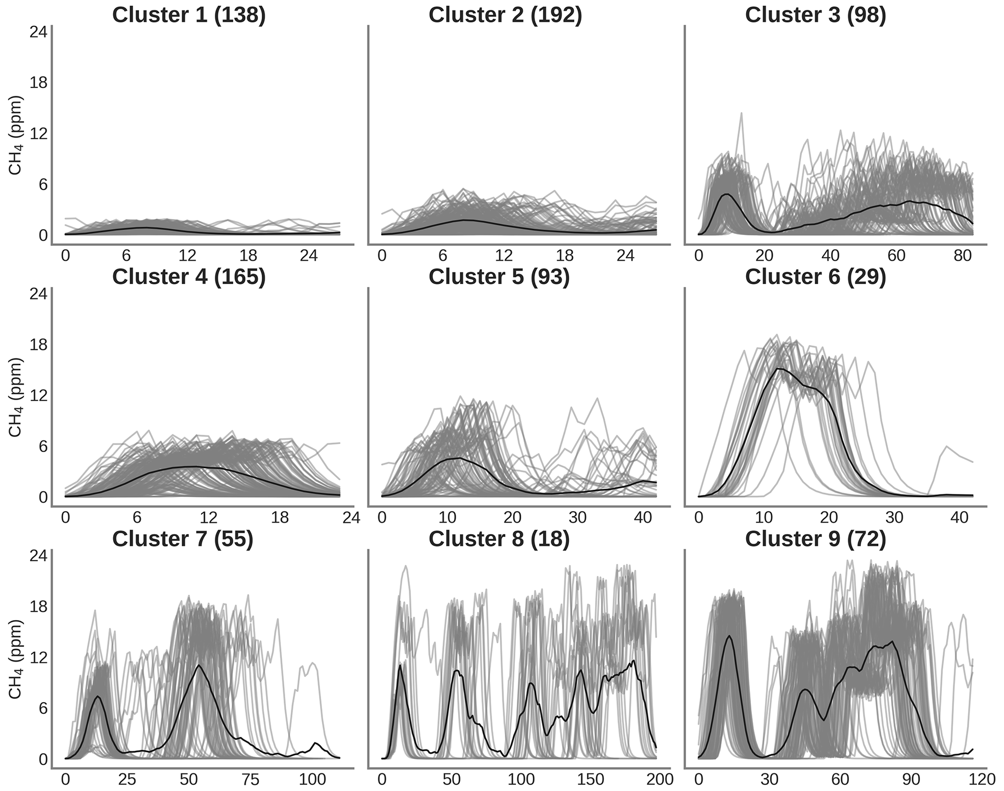
Figure A9 Clustering of peaks using DTW on the reference instrument for the same spikes detected by sensors on chamber C. On the title of each plot, the number inside the parentheses correspond to the number of spikes attributed to each cluster. Thin gray lines represent all the peaks inside each cluster, and the black line is the mean of all the peaks corresponding to each class.

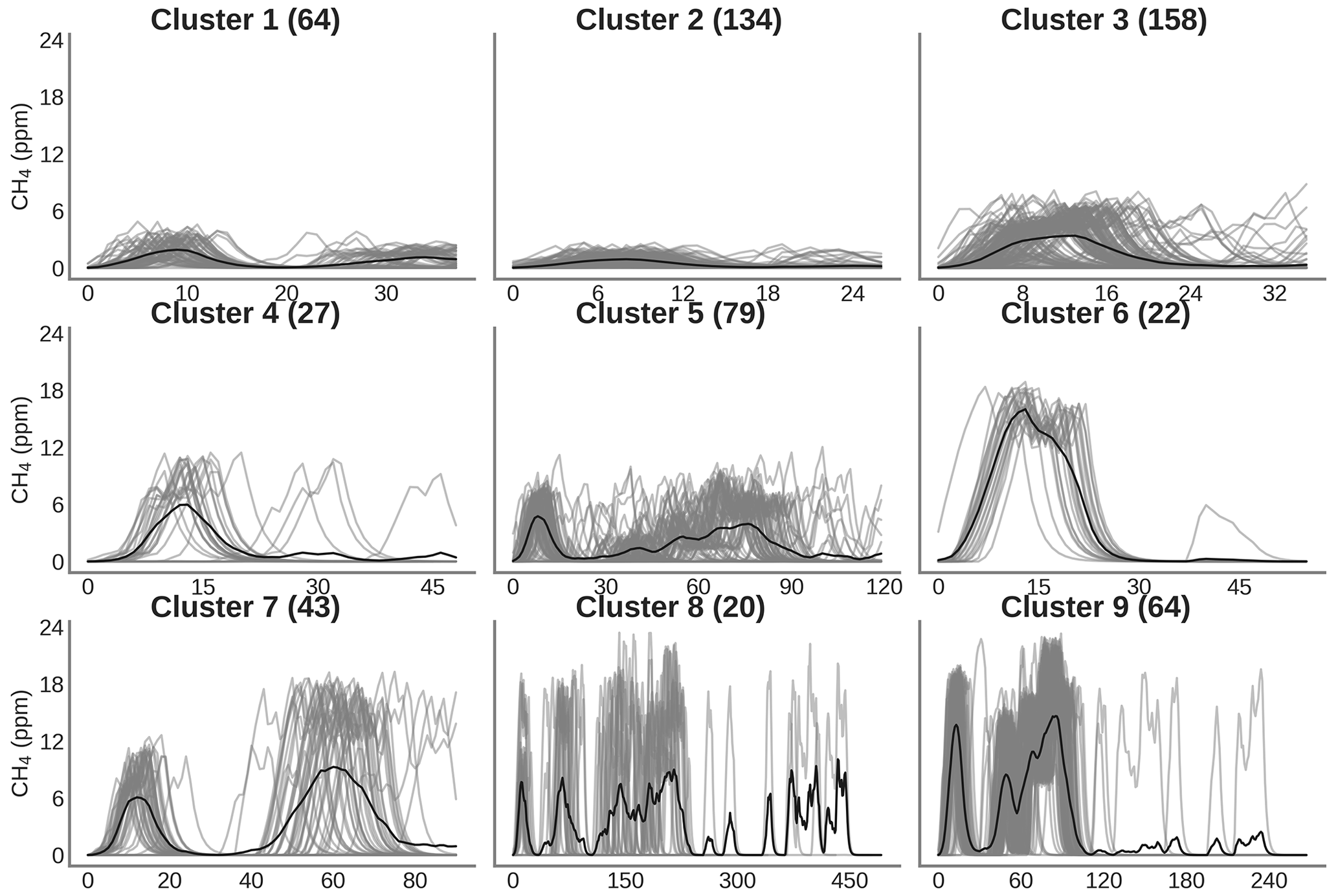
Figure A10 Clustering of peaks using DTW on the reference instrument for the same spikes detected by sensors on chamber D. On the title of each plot, the number inside the parentheses corresponds to the number of spikes attributed to each cluster. Thin gray lines represent all the peaks inside each cluster, and the black line is the mean of all the peaks corresponding to each class.

Table A1 MSD decomposition for the different configurations and both test set sizes considering only Figaro^® TGS sensors as input. Letters inside parentheses indicate the sensor used: TGS 2611-E00 is denoted by “E”, TGS2611-C00 is denoted by “C” and both sensors as input are denoted as “C&E”.

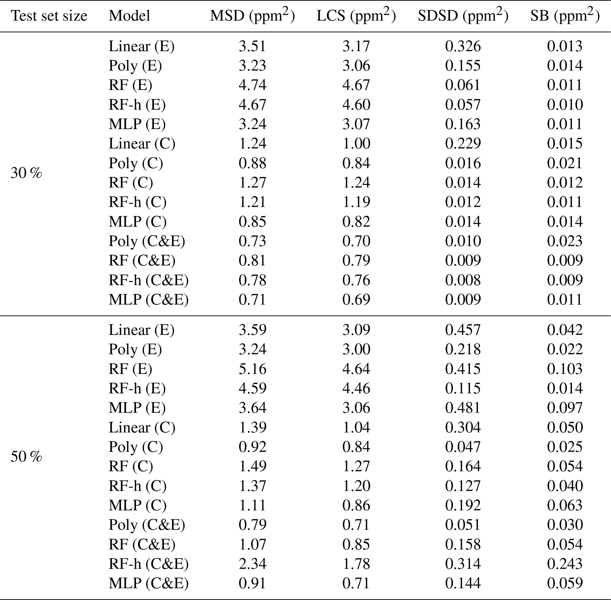
Table A2 MSD decomposition for the different configurations and both test set sizes considering Figaro^® TGS sensors and environmental variables as input. Notation is the same as in Table A1.

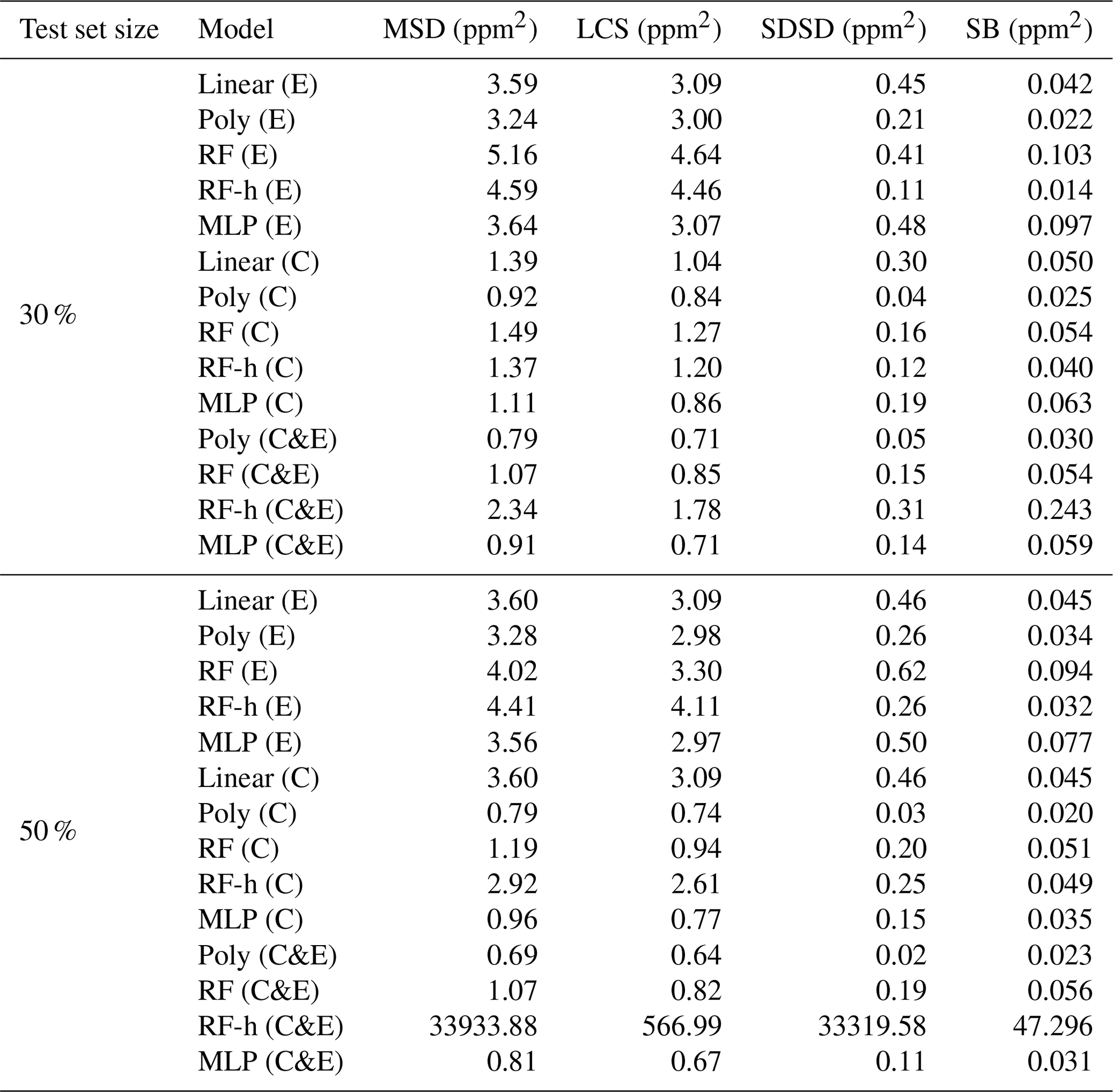
Table A3 RMSE (in ppm) for the different configurations of subsetting based on the selected clusters of peaks. Only Figaro^® sensors were used to compute this error. Each configuration is denoted “CX”, with X being the number of the configuration. In each row, the models are denoted with a letter inside parentheses to indicate the sensors used. “C” denotes the TGS 2611-C00, “E” the TGS 2611-E00 and “C&E” both sensors.

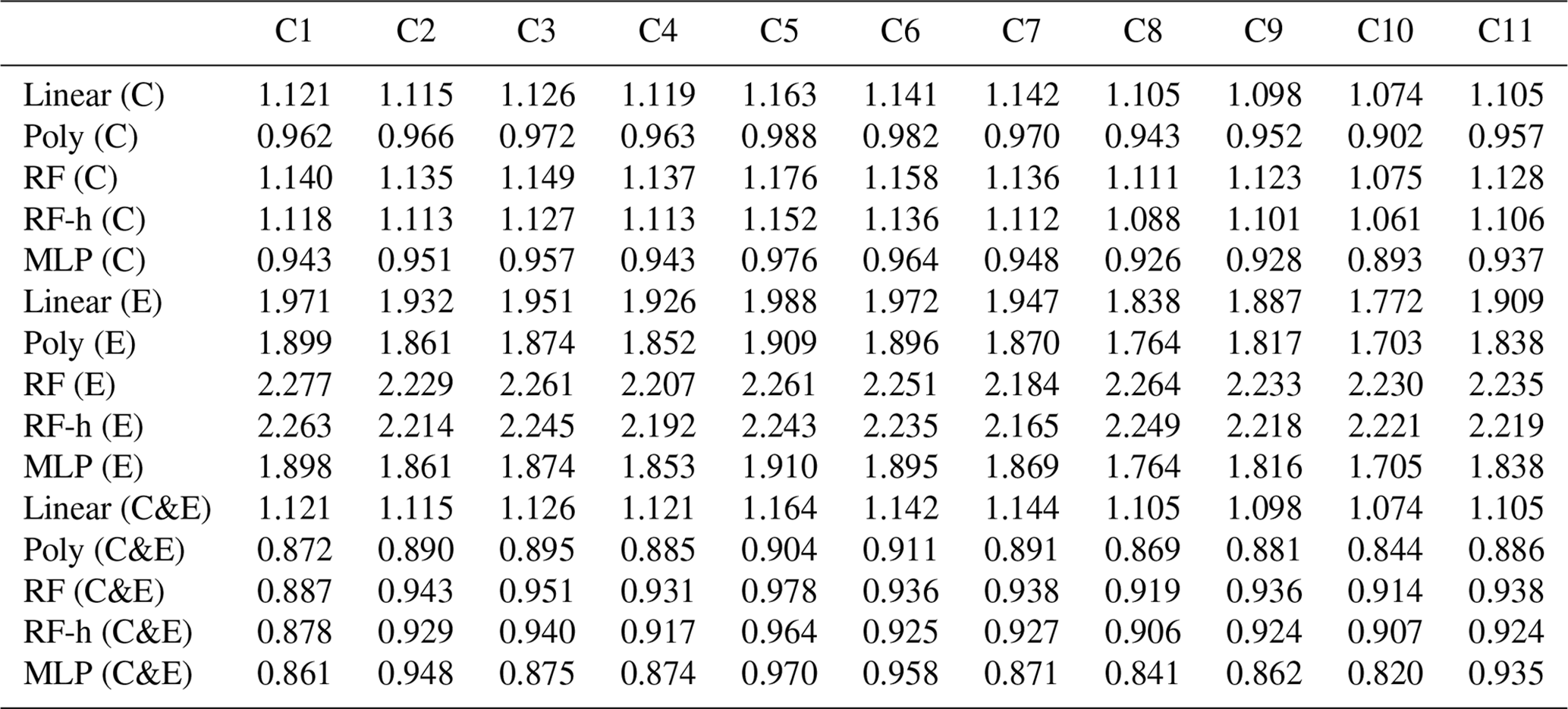
Table A4 RMSE (in ppm) for the different configurations of subsetting based on the selected clusters of peaks. Figaro^® sensors and environmental variables were used to compute this errors. Notation is the same as in Table A3.

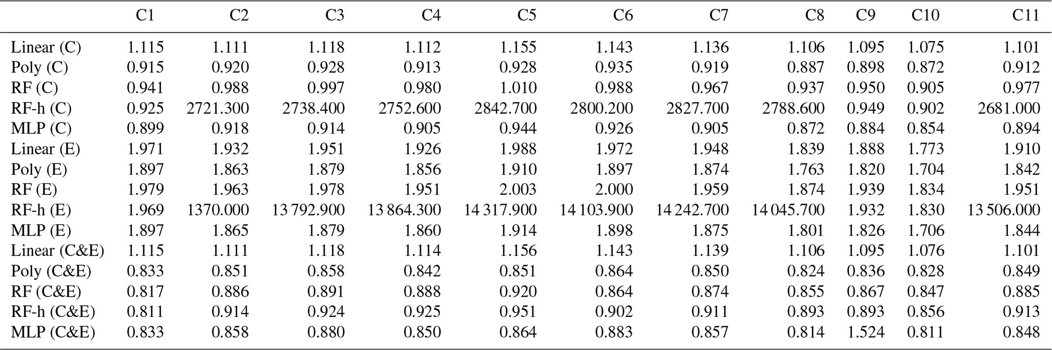
Table A5 Summary statistics of the Pearson correlation coefficient (ρ) distributions between models on the test set for a 20-fold cross-validation. The inputs of the modes are only voltage from the Figaro^® TGS sensors.

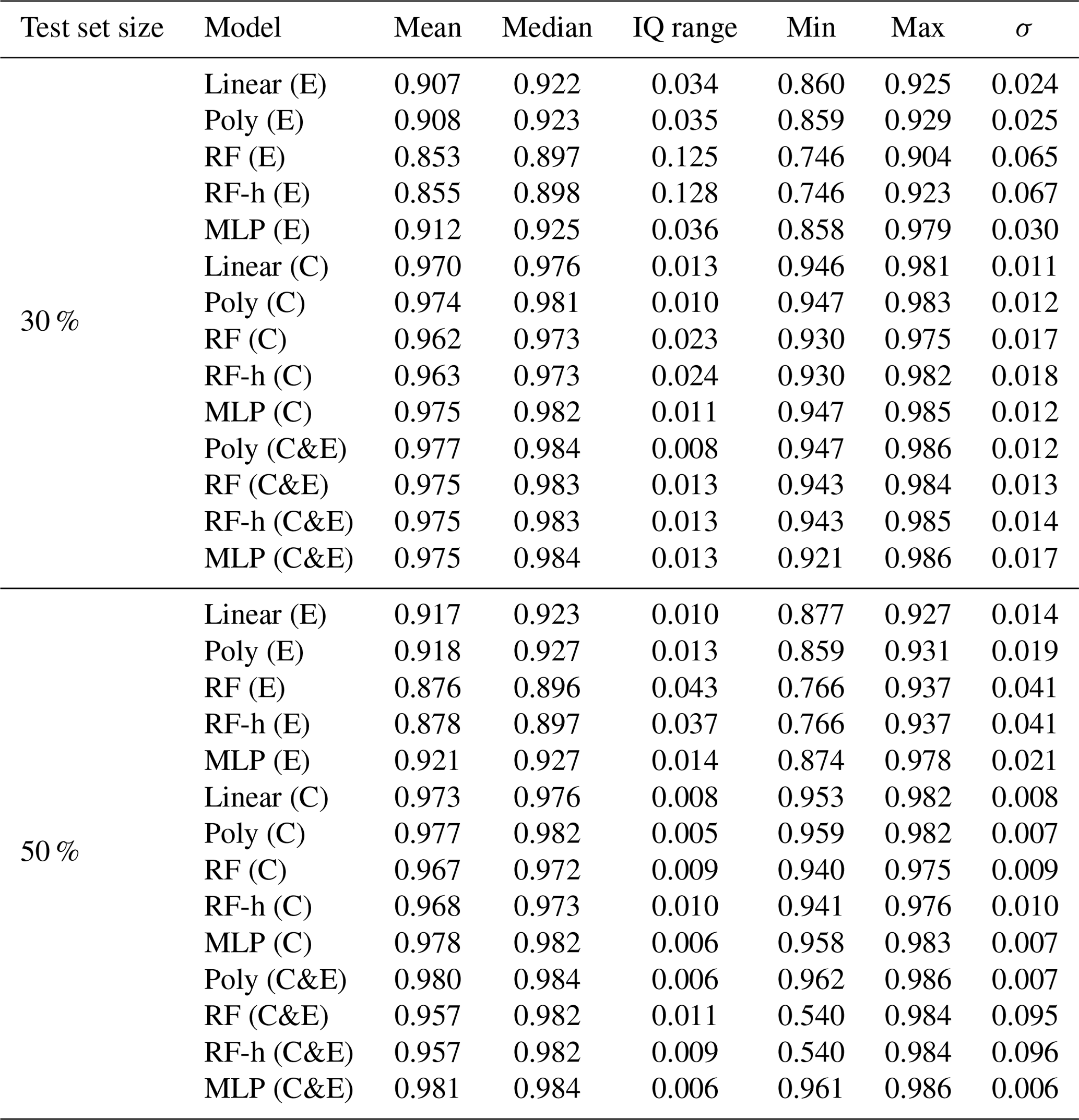
Table A6 Summary statistics of the Pearson correlation coefficient (ρ) distributions between models on the test set for a 20-fold cross-validation. The inputs of the models include voltage from low-cost sensors and environmental variables (H₂O, temperature and pressure).

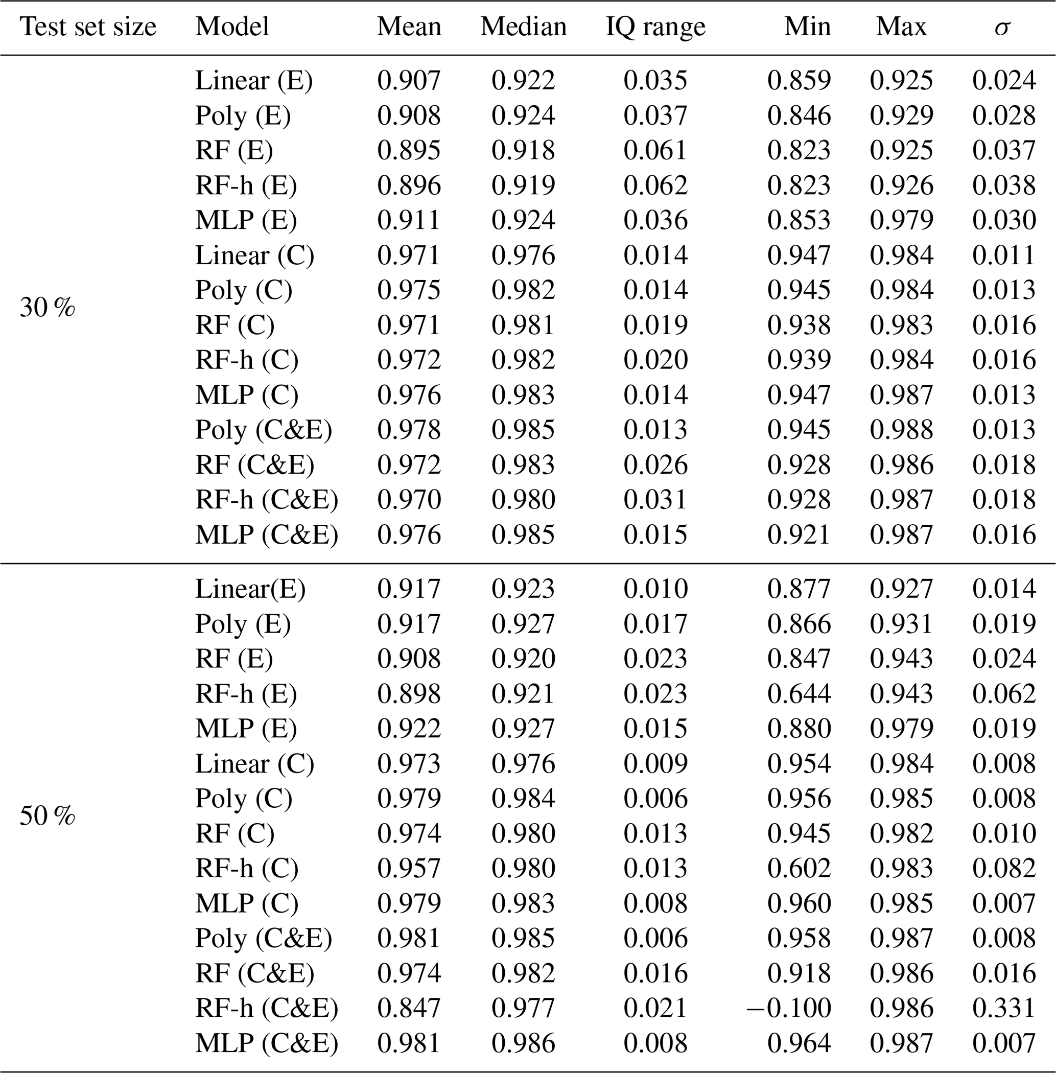
Table A7 Comparison between TGS sensors included in the low-cost logging system.