A flexible algorithm for network design based on information theory

A novel method for atmospheric network design is presented, which is based on information theory. The method does not require calculation of the posterior uncertainty (or uncertainty reduction) and is therefore computationally more efficient than methods that require this. The algorithm is demonstrated in two examples: the first looks at designing a network for monitoring CH₄ sources using observations of the stable carbon isotope ratio in CH₄ (δ¹³C), and the second looks at designing a network for monitoring fossil fuel emissions of CO₂ using observations of the radiocarbon isotope ratio in CO₂ (Δ¹⁴CO₂).

1 Introduction

The optimal design of any observing network is an important problem in order to maximize the information obtained with minimal cost. In atmospheric sciences, observing networks include those for weather prediction, as well as for air quality and the monitoring of greenhouse gases (GHGs). For air quality and GHGs, one essential purpose of the observation network is to learn about the underlying sources and, where relevant, the sinks. This application is based on inverse methodology in which knowledge about some unknown variables, in this case the sources (and sinks), can be determined by indirect observations, that is, the atmospheric concentrations or mixing ratios, if there is a model or function that relates the unknown variables to the observations. Inverse methodology provides a means to relate the observations to the unknown variables and provides an optimal estimate of these (Tarantola, 2005).

In atmospheric sciences, the methodology is most often derived from Bayes' theorem, which describes the conditional probability of the state variables, x, given the observations, y.

$$\begin{array}{}\text{(1)}& P\left(x|y\right)={\displaystyle \frac{P\left(y|x\right)P\left(x\right)}{P\left(y\right)}}\end{array}$$

Assuming a Gaussian probability density function (PDF), the following cost function can be derived (Rodgers, 2000).

$$\begin{array}{}\text{(2)}& \begin{array}{rl}J\left(\mathit{x}\right)& ={\displaystyle \frac{\mathrm{1}}{\mathrm{2}}}{\left(\mathit{x}-{\mathit{x}}_{\mathrm{b}}\right)}^{\mathrm{T}}{\mathbf{B}}^{-\mathrm{1}}\left(\mathit{x}-{\mathit{x}}_{\mathrm{b}}\right)\\ & +{\displaystyle \frac{\mathrm{1}}{\mathrm{2}}}{\left(\mathit{H}\left(\mathit{x}\right)-\mathit{y}\right)}^{\mathrm{T}}{\mathbf{R}}^{-\mathrm{1}}\left(\mathit{H}\left(\mathit{x}\right)-\mathit{y}\right)\end{array}\end{array}$$

The x for which J(x) is the minimum is the state vector that minimizes the sum of two distances: one in the observation space, between the modelled, H(x), and observed, y, variables, and the other in the state space, between x and a prior estimate of state variables, x_b. These two distances are weighted by the matrices R and B, which are, respectively, the observation error covariance and prior error covariance. Expressions for the centre and variance of the posterior PDF of x are given by e.g. Tarantola (2005).

The choice of the locations for the observations has important consequences for how well the state variables can be constrained. Increasing the number of observations will decrease the dependence of the solution on x_b, but where those observations are made is also a critical consideration and depends on how they relate to the state variables, as described by the transport operator, H(x). Here only the linear transport case is considered in which this operator can be defined as the matrix H.

In practical applications of network design, there is usually a predefined budget that would allow the establishment of a given number of sites, either to create a new network or to add to an existing one. The possible locations of sites are usually a predefined set, since these need to fulfil certain criteria, e.g. access to the electrical grid, internet connection, road access, an existing building on site to house instruments, and the agreement of the property owner, and may include having an existing tower if measurements are to be made above the surface layer. Thus, the question is often the following: which potential sites should be chosen to provide the most information about the sources and sinks?

The founding work on network design was actually in the field of seismology (Hardt and Scherbaum, 1994), but there are already a number of examples of network design in the framework of atmospheric monitoring in the scientific literature. An early example is the optimization of a global network for CO₂ observations to improve knowledge of the terrestrial CO₂ fluxes (Gloor et al., 2000; Patra and Maksyutov, 2002; Rayner et al., 1996). These studies dealt only with small dimensional problems, i.e. with few state variables, relatively low-frequency observations, and thus small B and H matrices, and the criteria by which the network was chosen involved minimizing the posterior uncertainty. Gloor et al. (2000)​​​​​​​ solved the problem using a Monte Carlo method (specifically simulated annealing), but they found this method took considerable time to converge and up to 5 × 10⁵ iterations were needed. Patra and Makysutov (2002) used a less computationally demanding approach, the incremental optimization method, which is based on the “divide and conquer” algorithm principle. In this method, the problem to solve is broken down into steps, i.e. sequentially choosing the best site from the set of potential sites and correspondingly depleting this set by one with each step. In the incremental optimization approach only $\sum _{i=\mathrm{1}}^k(p-i+\mathrm{1})$ calculations are needed, where k is the number of sites to select and p the number of potential sites to choose from. The incremental optimization approach, however, may lead to a different selection of sites compared to testing all possible combinations of sites, which would involve $p\mathrm{!}/\left(k\mathrm{!}\right(p-k\left)\mathrm{!}\right)$ calculations, but this in many cases may be a prohibitively large number.

More recently, the problem of network design has been addressed in the context of regional networks for GHG observations (Lucas et al., 2015; Nickless et al., 2015). Again, in both these studies the metric for selecting the network was the posterior uncertainty, either by using the trace of the posterior error covariance matrix, which is equivalent to minimizing the mean square uncertainty for all grid cells (Lucas et al., 2015), or by minimizing the sum of the posterior error covariance matrix (or submatrix for a particular region), which also accounts for the covariance of uncertainty between grid cells (Nickless et al., 2015). These studies both used Monte Carlo approaches (specifically, genetic algorithms) to find the network minimizing the selected metric.

However, for large problems any metric involving the posterior uncertainty becomes a bottleneck, if not unworkable, since the calculation of the posterior error covariance matrix, A, requires inverting the matrix ${\mathbf{H}}^{\mathrm{T}}{\mathbf{R}}^{-\mathrm{1}}\mathbf{H}+{\mathbf{B}}^{-\mathrm{1}}$ which has dimensions of n×n where n is the number of state variables. For this reason, methods were proposed based on criteria considering how well a network resolves the atmospheric variability or “signal” or, in other words, how well they sample regions of significant atmospheric heterogeneity (Shiga et al., 2013). In this approach, the atmospheric signal (e.g. mixing ratio) is modelled using an atmospheric transport model and a prior flux estimate, and sites are sequentially added to the network so that the distance of any grid cell from an observation site is within some predetermined correlation scale length. For this method, the number of calculation steps is equal to the sites to be selected (Shiga et al., 2013). Although computationally very efficient, this method does not consider the information gained about the state variables but only the optimal sampling of atmospheric variability.

An alternative method, but also based on the consideration of atmospheric variability, is to consider how “similar” the atmospheric signal is between potential sites in a network and to reduce the number of sites, leaving only those with significantly different signals (Risch et al., 2014). Risch et al. (2014)​​​​​​​ applied a clustering method to cluster sites with similar signals (i.e. strongly correlated sites), and individual sites were removed from each cluster based on the premise that they did not contribute any significant new information, whereas sites in clusters of one member were all retained. However, as in the method of Shiga et al. (2013), this approach does not consider the information gained about the state variables and how atmospheric transport alone may influence the variability at each site.

Here a method for network design is proposed based on information theory. This method requires precomputed transport operators for each potential site, so-called site “footprints” or “source–receptor relationships” (SRRs), which can be calculated directly using a Lagrangian atmospheric transport model (Seibert and Frank, 2004) or from forward calculations of an Eulerian transport model for each source (Rayner et al., 1999; Enting, 2002). The method can be applied to the problem of creating a new network or expanding an existing one and can be applied to observations of mixing ratios, isotopic ratios, column measurements, or a combination of these. It provides an alternative criterion to the posterior uncertainty (or uncertainty reduction) to assess a potential network and can be used with either incremental optimization or Monte Carlo approaches. It has a number of advantages compared to previous methods: (i) it does not require the inversion of any large matrix, except for B, but this is needed only once, making it computationally efficient; (ii) it accounts for spatial correlations in the state variables; and (iii) it allows for an exact formulation of the problem to be solved, i.e. what is the improvement in knowledge about the unknown variables. On the other hand, it requires linearity of the operator from the state space to the observation space, which is not the case for methods examining only atmospheric variability.

Two example applications are presented, which are based on real-life network design problems. The first considers adding measurements of the stable isotope ratio of CH₄, i.e. δ¹³C, to a subset of existing sites measuring CH₄ mixing ratios in order to maximize the information about CH₄ sources. The second considers designing a network for Δ¹⁴CO₂ measurements to maximize the information about fossil fuel emissions of CO₂.

2 Methodology

In information theory, the information content of a measurement can be thought of as the amount by which knowledge of some variable is improved by making the measurement, and the entropy is the level of information contained in the measurement (Rodgers, 2000). In this case, one can consider the PDF a measure of knowledge about the state variables, and the information provided by a measurement can be found by comparing the entropy of the PDFs before and after measurement was made. Furthermore, the information content of the measurement is equal to the reduction in entropy. In the application of network design, all observations within the potential network are considered to be one “measurement”.

The entropy, S, of the PDF given by P(x) is

$$\begin{array}{}\text{(3)}& S\left(P\left(x\right)\right)=-\int P\left(x\right)\ln \left(P\left(x\right)\right).\end{array}$$

And the information content, I, is the reduction in entropy after a measurement is made:

$$\begin{array}{}\text{(4)}& I=S\left(P\left(x\right)\right)-S\left(P\left(\left(x|y\right)\right)\right),\end{array}$$

where P(x) is the prior PDF (before measurement) and P(x|y) is the posterior PDF (after the measurement, y). The entropy is given by integrating Eq. (3) over the bounds −∞ to +∞ (Rodgers, 2000), which for a Gaussian PDF of a scalar variable is

$$\begin{array}{}\text{(5)}& S=\ln \left(\mathit{\sigma }{\left(\mathrm{2}\mathit{\pi }e\right)}^{\frac{\mathrm{1}}{\mathrm{2}}}\right),\end{array}$$

where σ is the standard deviation. In the multivariate case with m variables the entropy is given by

$$\begin{array}{}\text{(6)}& S=\sum _{i=\mathrm{1}}^m\ln {\left(\mathrm{2}\mathit{\pi }e{\mathit{\lambda }}_i\right)}^{\frac{\mathrm{1}}{\mathrm{2}}},\end{array}$$

where λ_i is an eigenvalue of the error covariance matrix. By rearrangement one can write the following.

$$\begin{array}{}\text{(7)}& {\displaystyle }S=\sum _{i=\mathrm{1}}^m\left(\ln {\left(\mathrm{2}\mathit{\pi }e\right)}^{\frac{\mathrm{1}}{\mathrm{2}}}+\ln {\mathit{\lambda }}_i^{\frac{\mathrm{1}}{\mathrm{2}}}\right),\text{(8)}& {\displaystyle }S=m\ln {\left(\mathrm{2}\mathit{\pi }e\right)}^{\frac{\mathrm{1}}{\mathrm{2}}}+{\displaystyle \frac{\mathrm{1}}{\mathrm{2}}}\ln \left(\prod {\mathit{\lambda }}_i\right),\text{(9)}& {\displaystyle }S=m\ln {\left(\mathrm{2}\mathit{\pi }e\right)}^{\frac{\mathrm{1}}{\mathrm{2}}}+{\displaystyle \frac{\mathrm{1}}{\mathrm{2}}}\ln \left|\mathbf{B}\right|\end{array}$$

In Eq. 9 $\left|\mathbf{B}\right|$ is the determinant of the prior error covariance matrix, using the fact that the determinant of a symmetric matrix is equal to the product of its eigenvalues. Similarly, the entropy for the posterior PDF can be derived, giving the information content as

$$\begin{array}{}\text{(10)}& I={\displaystyle \frac{\mathrm{1}}{\mathrm{2}}}\ln \left|\mathbf{B}\right|-{\displaystyle \frac{\mathrm{1}}{\mathrm{2}}}\ln \left|\mathbf{A}\right|,\end{array}$$

where A is the posterior error covariance matrix. In this case the determinant can be thought of as defining the volume in state space occupied by the PDF, which describes the knowledge about the state; thus, I is the change in the log of the volume when observation is made. From Eq. (10) one can derive the following.

$$\begin{array}{}\text{(11)}& I={\displaystyle \frac{\mathrm{1}}{\mathrm{2}}}\ln \left|{\mathbf{BA}}^{-\mathrm{1}}\right|\end{array}$$

And given that the inverse of A is equal to the Hessian matrix of J(x) (Eq. 2)

$$\begin{array}{}\text{(12)}& {\mathbf{A}}^{-\mathrm{1}}={\mathbf{H}}^{\mathrm{T}}{\mathbf{R}}^{-\mathrm{1}}\mathbf{H}+{\mathbf{B}}^{-\mathrm{1}},\end{array}$$

one obtains

$$\begin{array}{}\text{(13)}& I={\displaystyle \frac{\mathrm{1}}{\mathrm{2}}}\ln \left|{\mathbf{BH}}^{\mathrm{T}}{\mathbf{R}}^{-\mathrm{1}}\mathbf{H}+\mathbf{I}\right|,\end{array}$$

where R is the observation error covariance matrix, H is the model operator (for atmospheric observations it is the atmospheric transport operator), and I is the identity matrix.

The principle of this network design method is to choose the sites that maximize the information, and this criterion can be used in either the incremental optimization or Monte Carlo approach. The incremental optimization approach is computationally efficient, requiring only $\sum _{i=\mathrm{1}}^k(p-i+\mathrm{1})$ calculations and delivers, if not the same, at least similar results as testing all possible combinations of sites (Patra and Maksyutov, 2002).

The calculation of the matrix ${\mathbf{BH}}^{\mathrm{T}}{\mathbf{R}}^{-\mathrm{1}}\mathbf{H}+\mathbf{I}$ can be quite fast, since H and R can be made quite small. H does not need to represent all observations for each site, but only the average observation corresponding to different levels of uncertainty or “characteristic observations”. In the case that observations at each site have only one characteristic uncertainty, then H will have dimension k×n where n is the number of state variables, and R will be k×k; in practice R is most often diagonal. In the case that the uncertainty of an observation at a given site varies depending on when it was made, e.g. daytime or nighttime, then the dimension of H will be 2k×n. The computationally demanding step is the calculation of the matrix determinant. However, this calculation can be made very efficient if the matrix ${\mathbf{BH}}^{\mathrm{T}}{\mathbf{R}}^{-\mathrm{1}}\mathbf{H}+\mathbf{I}$ is decomposed into B and (${\mathbf{H}}^{\mathrm{T}}{\mathbf{R}}^{-\mathrm{1}}\mathbf{H}+{\mathbf{B}}^{-\mathrm{1}}$), which are both symmetric positive definite matrices, and using the fact that the log of the determinant of a symmetric positive definite matrix can be calculated as the trace of the log of the lower triangular matrix of the Cholesky decomposition:

$$\begin{array}{}\text{(14)}& {\displaystyle }I& {\displaystyle }={\displaystyle \frac{\mathrm{1}}{\mathrm{2}}}\ln \left(\left|\mathbf{B}\right|\right)+{\displaystyle \frac{\mathrm{1}}{\mathrm{2}}}\ln \left(\left|{\mathbf{H}}^{\mathrm{T}}{\mathbf{R}}^{-\mathrm{1}}\mathbf{H}+{\mathbf{B}}^{-\mathrm{1}}\right|\right)\text{(15)}& {\displaystyle }& {\displaystyle }=\mathrm{tr}\left(\ln \left(\mathbf{L}\right)\right)+\mathrm{tr}\left(\ln \left(\mathbf{M}\right)\right),\end{array}$$

where B=LL^T and ${\mathbf{H}}^{\mathrm{T}}{\mathbf{R}}^{-\mathrm{1}}\mathbf{H}+{\mathbf{B}}^{-\mathrm{1}}={\mathbf{MM}}^{\mathrm{T}}$ where L and M are the lower triangular matrices. Note that if temporal correlations in B can be ignored, then B only needs to be formulated for a single time step, i.e. B_t, which is a considerably smaller matrix than B, and ${\mathbf{H}}^{\mathrm{T}}{\mathbf{R}}^{-\mathrm{1}}\mathbf{H}+{\mathbf{B}}^{-\mathrm{1}}$ can be calculated stepwise adding ${\mathbf{B}}_t^{-\mathrm{1}}$ for each time step. Furthermore, ${\mathbf{B}}_t^{-\mathrm{1}}$ (or B⁻¹) only needs to be calculated once, since it does not change with choice of sites. In this case the information content is simply

$$\begin{array}{}\text{(16)}& I=q\mathrm{tr}\left(\ln \left(\mathbf{L}\right)\right)+\mathrm{tr}\left(\ln \left(\mathbf{M}\right)\right),\end{array}$$

where q is the number of time steps and L in this case is the lower triangular matrix of B_t.

The computational complexity of the whole algorithm can be estimated considering that the Cholesky decomposition of a symmetric matrix has a complexity of $O\left(n^{\mathrm{3}}\right)/\mathrm{3}$. The calculation of B⁻¹ from B requires $O\left(n^{\mathrm{3}}\right)/\mathrm{3}$ operations. The calculation of R⁻¹ from R requires $O\left(k^{\mathrm{3}}\right)/\mathrm{3}$ operations. The calculation of H^TR⁻¹H requires $O(n{k}^{\mathrm{2}}+n^{\mathrm{2}}k)\sim O\left(n^{\mathrm{2}}\right)$ operations if k≪n. Then only the calculation of the determinant of the matrix $\left|{\mathbf{H}}^{\mathrm{T}}{\mathbf{R}}^{-\mathrm{1}}\mathbf{H}+{\mathbf{B}}^{-\mathrm{1}}\right|$ remains, which given that it is symmetric and positive definite also takes $O\left(n^{\mathrm{3}}\right)/\mathrm{3}$ operations (Aho et al., 1974). The subsequent logarithm and the trace operations are linear with respect to n, i.e. O(n). The total complexity yields $O\left(n^{\mathrm{3}}\right)/\mathrm{3}+O\left(k^{\mathrm{3}}\right)/\mathrm{3}+O\left(n^{\mathrm{2}}\right)+O\left(n^{\mathrm{3}}\right)/\mathrm{3}+O\left(n\right)\approx \mathrm{2}O\left(n^{\mathrm{3}}\right)/\mathrm{3}+O\left(k^{\mathrm{3}}\right)/\mathrm{3}$, which is comparable to e.g. one n×n LU factorization if k≪n.

3 Examples

3.1 Enhancing a network for estimating sources of CH₄

This example considers the enhancement of a network of atmospheric measurements of CH₄ mixing ratios by adding observations of stable isotopic ratios, δ¹³C, at a selected number of sites within the existing network in order to improve knowledge of the different CH₄ sources. For the example, the case of the Integrated Carbon Observation System (ICOS) network (https://www.icos-cp.eu, last access: 12 January 2023) in Europe is used, which consists of 24 operational sites in geographical Europe measuring CH₄ mixing ratios (Table 1). In this hypothetical case, the budget is available to equip 5 of the 24 sites with in situ instruments measuring δ¹³C at hourly frequency, as is now possible with modern instrumentation (Menoud et al., 2020). The problem can thus be formulated as follows: given the existing information provided by 24 sites measuring CH₄ mixing ratios, which sites are the best to choose for the additional δ¹³C observations?

Table 1 List of sites in the ICOS network (only those in geographical Europe are included). The sampling height that was used in this study is shown, which is the highest sampling height at each site.

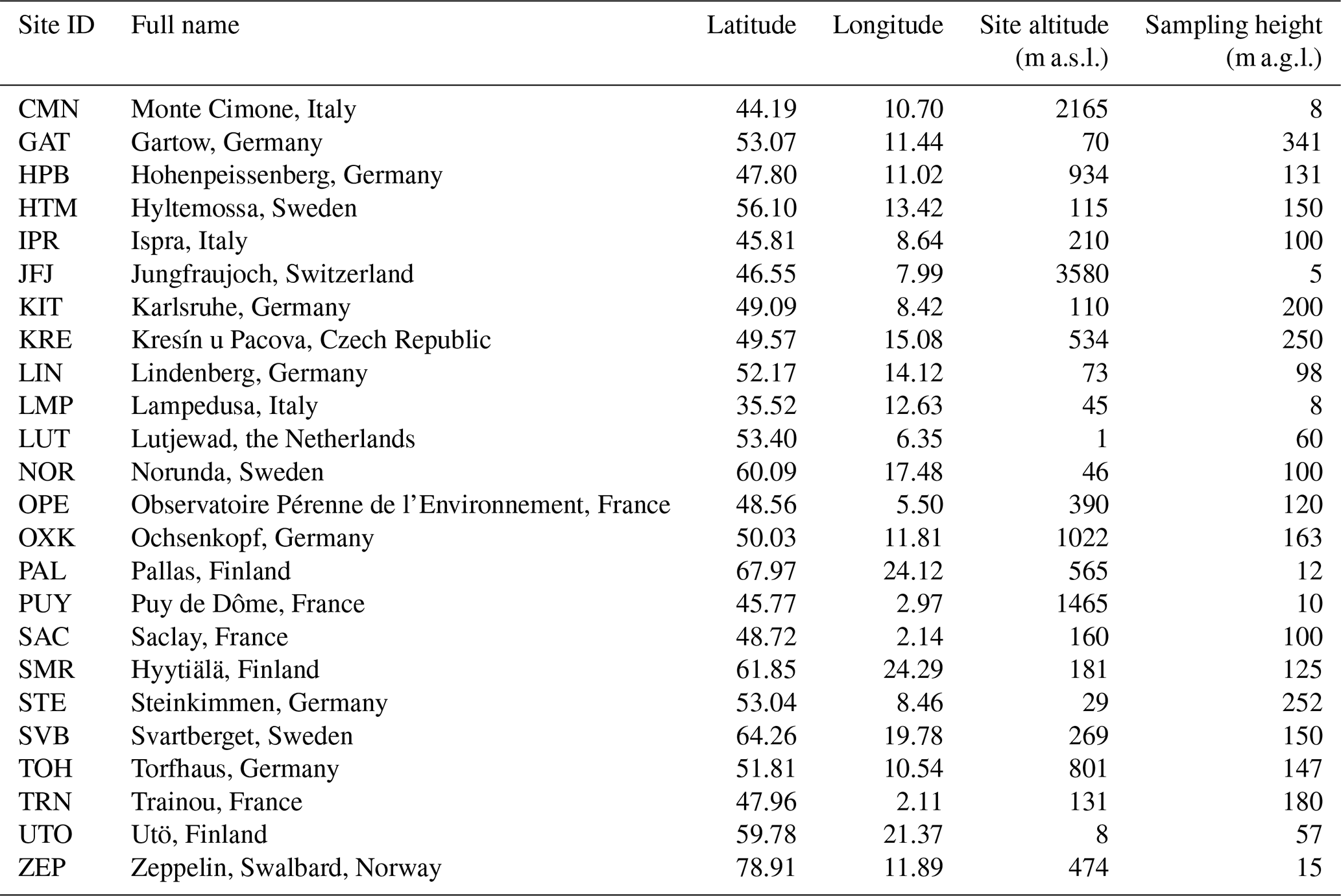
Table 2 The prior fluxes and δ¹³C value used for each source where the total and mean δ¹³C values are given for the European domain.

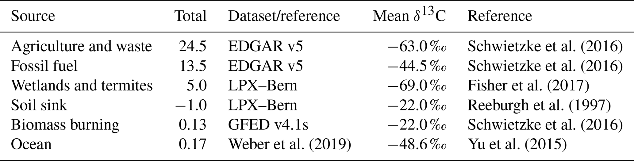
The δ¹³C value is the ratio of ¹³C to ¹²C in a sample relative to a reference value measured in per mil (‰).

$$\begin{array}{}\text{(17)}& {\mathit{\delta }}^{\mathrm{13}}\mathrm{C}=\left({\displaystyle \frac{R_{\mathrm{sam}}}{R_{\mathrm{ref}}}}-\mathrm{1}\right)\times \mathrm{1000}\end{array}$$

The δ¹³C value in the atmosphere varies as a result of variations in the δ¹³C value of the sources, the oxidation of CH₄ in the atmosphere and in soils, and atmospheric transport. Sources of CH₄ can be grouped according to their characteristic δ¹³C value, with microbial sources being the most depleted in ¹³C, while thermogenic sources such as from oil, gas, and coal are less depleted, and pyrogenic sources, such as biomass burning, are the least depleted (Fisher et al., 2011; Dlugokencky et al., 2011; Brownlow et al., 2017) (Table 2). In this example, CH₄ sources were grouped into anthropogenic microbial sources, namely agriculture and waste (agw); fossil sources, namely fossil fuel and geological emissions (fos); biomass burning sources (bbg); and natural microbial sources, principally wetlands (wet) and the ocean source (oce). The change in CH₄ mixing ratios from all sources can thus be written as

$$\begin{array}{}\text{(18)}& \mathrm{\Delta }c=\mathbf{H}{\mathit{x}}_{\mathrm{agw}}+\mathbf{H}{\mathit{x}}_{\mathrm{wet}}+\mathbf{H}{\mathit{x}}_{\mathrm{fos}}+\mathbf{H}{\mathit{x}}_{\mathrm{bbg}}+\mathbf{H}{\mathit{x}}_{\mathrm{oce}},\end{array}$$

where Δc is the change in CH₄ mixing ratios, x is the vector of fluxes, and H is the transport operator. Analogously, the change in δ¹³C can be defined as

$$\begin{array}{}\text{(19)}& \begin{array}{rl}\mathrm{\Delta }{\mathit{\delta }}^{\mathrm{13}}c& =\mathbf{H}{\mathit{\delta }}_{\mathrm{agw}}{\mathit{x}}_{\mathrm{agw}}+\mathbf{H}{\mathit{\delta }}_{\mathrm{wet}}{\mathit{x}}_{\mathrm{wet}}+\mathbf{H}{\mathit{\delta }}_{\mathrm{fos}}{\mathit{x}}_{\mathrm{fos}}\\ & +\mathbf{H}{\mathit{\delta }}_{\mathrm{bbg}}{\mathit{x}}_{\mathrm{bbg}}+\mathbf{H}{\mathit{\delta }}_{\mathrm{oce}}{\mathit{x}}_{\mathrm{oce}},\end{array}\end{array}$$

where δ_x is the isotopic signature for each source type. Therefore, the transport operator for an observation of the change in δ¹³C is just the transport operator H but scaled by δ_x for each source.

For this example, SRRs were calculated for all 24 sites in the ICOS network using the Lagrangian particle dispersion model, FLEXPART (Pisso et al., 2019), driven with ERA-Interim reanalysis wind fields. Retro-plumes were calculated for 10 d backwards in time from each site at an hourly frequency. The SRRs were saved at 0.5^∘ × 0.5^∘ resolution over the European domain of 12^∘ W to 32^∘ E and 35 to 72^∘ N and averaged over all observations within a month to give a monthly mean SRR for each site.

The uncertainty in the δ¹³C measurements was set to the same value for each site, that is, at 0.07 ‰ based on experimental values (Menoud et al., 2020). Similarly, the uncertainty in CH₄ mixing ratio measurements was also set to the same value at all sites, at 5 ppb (WMO, 2009). The prior uncertainty σ for each grid cell was calculated as 0.5 times the prior flux, with a lower threshold equal to the first percentile value of all grid cells with non-zero flux for the smallest flux source. The spatial correlation between grid cells was calculated based on exponential decay over distance with a correlation scale length of 250 km over land. The prior error covariance matrix was then calculated as

$$\begin{array}{}\text{(20)}& \mathbf{B}=\mathbf{\Sigma }\mathbf{C}\mathbf{\Sigma },\end{array}$$

where C is the spatial correlation matrix and Σ is a diagonal matrix with the diagonal terms equal to the prior uncertainties for each grid cell.

For this example, the optimal network was found for three different scenarios: (1) monitoring all sources in EU27 countries plus the UK, Norway, and Switzerland (EU27 + 3); (2) monitoring only anthropogenic sources in EU27 + 3; and (3) as in scenario 1 but ignoring the existing information provided by CH₄ mixing ratios at all sites.

For these scenarios the influence of the fluxes that are not the target of the network needs to be projected into the observation space and included in the R matrix. For example, in scenario 1 this is the influence of fluxes outside EU27 + 3, and in scenario 2 it is the influence of all non-anthropogenic sources plus the influence of fluxes outside EU27 + 3. This is calculated as

$$\begin{array}{}\text{(21)}& \mathbf{R}={\mathbf{HB}}_{\mathrm{other}}{\mathbf{H}}^{\mathrm{T}}+{\mathbf{R}}_{\mathrm{meas}},\end{array}$$

where R_meas is simply the prior measurement uncertainty and B_other is the prior error covariance matrix for the other (i.e. non-target) fluxes.

For all scenarios the choice of the first four optimal sites was the same, that is, IPR, SAC, KIT, and LIN, while the last site chosen was KRE in scenarios 1 and 2 (Fig. 1) and LUT in scenario 3. All chosen sites are strongly sensitive to anthropogenic emissions, and the choice to optimize all sources or only anthropogenic sources made no difference in this example, likely because the natural sources (predominantly wetlands) are a relatively small contribution to the total CH₄ source in Europe (only 12 %). On the other hand, ignoring existing information provided by CH₄ mixing ratios led to LUT being chosen over KRE, likely because LUT provides a stronger constraint on the region with the largest emissions and diverse sources, i.e. Benelux (Fig. 2), which is more important in the absence of CH₄ mixing ratio data.

Figure 1 Map of the total mean SRRs for optimal sites for scenarios 1 and 2. Since only the EU27 + 3 emissions are constrained, the SRRs are also only shown for EU27 + 3. The locations of the optimal sites are indicated by the white points (i.e. IPR, SAC, KIT, LIN, and KRE), and the locations of the unselected sites are indicated by the black points.

Figure 2 Map of annual mean CH₄ emissions (units of kg m⁻² yr⁻¹) plotted with a logarithmic (base of 2) colour scale.

3.2 Network of ¹⁴CO₂ measurements for fossil fuel emissions

This example concerns the establishment of a network for measurements of radiocarbon dioxide, ¹⁴CO₂, which can be used as a tracer for fossil fuel CO₂ emissions; since fossil fuel contains no ¹⁴C, its combustion depletes the atmospheric background value of ¹⁴CO₂ (Turnbull et al., 2009). Similar to the previous example, the ICOS network is used, which also has CO₂ measurements at 24 sites in Europe. The hypothetical problem can be formulated as follows: if there is a budget to equip 10 sites in the ICOS network with weekly flask samples for ¹⁴CO₂ analysis, which sites should be chosen to gain the most knowledge of fossil fuel emissions? In this case, only weekly measurement frequency is examined as ¹⁴CO₂ measurements cannot be made continuously, and the measurement method, either via counting radioactive decay or by accelerator mass spectrometry, is costly and time-consuming. The optimization problem needs to consider the information already brought by the CO₂ measurements at all sites (in this example hourly measurements) and, in addition, the influence on the atmospheric signal from other sources, which may change the sensitivity of a site to fossil fuel emissions.

Measurements of ¹⁴CO₂ are reported as the ratio of ¹⁴CO₂ to CO₂ relative to a reference ratio and given in units of per mil (‰).

$$\begin{array}{}\text{(22)}& {\mathrm{\Delta }}^{\mathrm{14}}\mathrm{C}=\left({\displaystyle \frac{R_{\mathrm{sam}}}{R_{\mathrm{ref}}}}-\mathrm{1}\right)\times \mathrm{1000}\end{array}$$

Since fossil fuels contain no ¹⁴C, its isotopic ratio is −1000 ‰. Other than fossil fuels, atmospheric values of Δ¹⁴CO₂ are determined by the natural production of ¹⁴CO₂ in the stratosphere, nuclear power and spent fuel-processing plants, ocean and land biosphere fluxes, and atmospheric transport. Ocean fluxes affect ¹⁴CO₂, since the ocean is not in isotopic equilibrium with the atmosphere owing to higher values of atmospheric ¹⁴CO₂ in the past due to nuclear bomb testing and similarly for plant respiration fluxes of CO₂ (Bozhinova et al., 2014).

The change in CO₂ mixing ratios can be described as follows:

$$\begin{array}{}\text{(23)}& \mathrm{\Delta }c=\mathbf{H}{\mathit{x}}_{\mathrm{fos}}+\mathbf{H}{\mathit{x}}_{\mathrm{pho}}+\mathbf{H}{\mathit{x}}_{\mathrm{res}}+\mathbf{H}{\mathit{x}}_{\mathrm{oce}},\end{array}$$

where x_fos is the fossil fuel emission, x_pho the land biosphere photosynthesis flux, x_res the land biosphere respiration flux, and x_oce the net ocean flux. A similar expression for the change in Δ¹⁴CO₂ can be derived following Bozhinova et al. (2014) as

$$\begin{array}{}\text{(24)}& \begin{array}{rl}{\mathrm{\Delta }}^{\mathrm{14}}c& =\mathbf{H}{\mathrm{\Delta }}_{\mathrm{fos}}{\mathit{x}}_{\mathrm{fos}}+\mathbf{H}{\mathrm{\Delta }}_{\mathrm{pho}}{\mathit{x}}_{\mathrm{pho}}+\mathbf{H}{\mathrm{\Delta }}_{\mathrm{res}}{\mathit{x}}_{\mathrm{res}}\\ & +\mathbf{H}{\mathrm{\Delta }}_{\mathrm{oce}}{\mathit{x}}_{\mathrm{oce}}+\mathbf{H}{\mathrm{\Delta }}_{\mathrm{nuc}}{\mathit{x}}_{\mathrm{nuc}},\end{array}\end{array}$$

where Δ¹⁴c is the change in Δ¹⁴CO₂, the term Δ_x is the isotopic signature of the corresponding source, and HΔ_nucx_nuc is the production of ¹⁴CO₂ from nuclear facilities. There is a term missing from Eqs. (23) and (24), namely the stratospheric production of CO₂ and ¹⁴CO₂. This term is ignored as the direct stratospheric contribution is negligible for the time and space domain considered by the Lagrangian model, since the observations are close to the surface. Equation (24) can be further simplified by removing the term HΔ_phox_pho, since photosynthesis, although it affects the ¹⁴CO₂ mixing ratio, does not affect Δ¹⁴CO₂ (Turnbull et al., 2009). Furthermore, the ocean and respiration fluxes can be split into a background term and a disequilibrium term, Δ_bg+Δ_ocedis and Δ_bg+Δ_resdis, respectively. As for photosynthesis, the background terms for ocean and respiration fluxes do not change Δ¹⁴CO₂, but only the disequilibrium terms change Δ¹⁴CO₂. For the domain in consideration, these terms are much smaller than that of fossil fuels and are ignored as in Bozhinova et al. (2014). With these simplifications, Eq. (24) becomes the following.

$$\begin{array}{}\text{(25)}& {\mathrm{\Delta }}^{\mathrm{14}}c=\mathbf{H}{\mathrm{\Delta }}_{\mathrm{fos}}{\mathit{x}}_{\mathrm{fos}}+\mathbf{H}{\mathrm{\Delta }}_{\mathrm{nuc}}{\mathit{x}}_{\mathrm{nuc}}\end{array}$$

Since x_nuc is pure ¹⁴CO₂, Δ_nuc would be infinite; therefore, the approach of Bozhinova et al. (2014) is used and Δ_nuc is approximated as the ratio of the activity of the sample and the referenced standard, giving ${\mathrm{\Delta }}_{\mathrm{nuc}}\approx \mathrm{0.7}\times {\mathrm{10}}^{\mathrm{15}}$ ‰.

Because, in this example, only the fossil fuel emissions are the unknown variables and the target of the network, the matrix B corresponds only to the uncertainty in the fossil fuel emissions and is resolved monthly. The other terms influencing CO₂ and Δ¹⁴CO₂ are projected into the observation space and included in the R matrix using Eq. (21). For the Δ¹⁴CO₂ observations, B_other is only the nuclear source, and for CO₂ observations, B_other includes photosynthesis and respiration, the sum of which is net ecosystem exchange (NEE) and the ocean flux, for which the effect on the observed CO₂ signal is very small and is thus ignored here. For both NEE and nuclear emissions, an uncertainty of 0.5 times the value in each grid cell was used to calculate B_other with a spatial correlation length of 250 km. Since NEE fluxes have large diurnal and seasonal cycles which co-vary with atmospheric transport, for the CO₂ observations, R was calculated using H and B, resolved for day, night, and monthly. Note, only one uncertainty value was calculated for each site, which represents the annual mean uncertainty for a daytime observation. Each site has a different uncertainty for CO₂ mixing ratios and Δ¹⁴CO₂ depending on the influence of NEE fluxes and nuclear emissions, respectively. This can be simply interpreted in terms of a signal-to-noise ratio. For example, for CO₂ mixing ratios where there is a large influence of NEE, the time series becomes noisier, similarly for the influence of nuclear emissions on Δ¹⁴CO₂ observations. The measurement uncertainty, R_meas, was set to the same value for each site, that is, at 2 ‰ for Δ¹⁴CO₂ (Turnbull et al., 2007) and 0.05 ppm for CO₂ mixing ratio measurements (WMO, 2018).

For this example, SRRs were calculated for all 24 sites in the ICOS network using FLEXPART with retro-plumes calculated for 5 d backwards in time from each site at an hourly frequency. The SRRs were saved at 0.5^∘ × 0.5^∘ and 3-hourly resolutions over the European domain of 15^∘ W to 35^∘ E and 30 to 75^∘ N and were averaged to give mean day and night SRRs for each month for each site. Estimates of NEE fluxes were used from the Simple Biosphere Model – Carnegie Ames Stanford Approach (SiBCASA) and were resolved 3-hourly (Schaefer et al., 2008), estimates of nuclear emissions were used from the CO₂ human emissions (CHE) project (Potier et al., 2022) and were an annual climatology, and estimates of fossil fuel emissions were from GridFED at monthly resolution (Jones et al., 2020a).

Figure 3 shows the uncertainty in the observation space at each site due to the influence of uncertainties in NEE and nuclear emissions on CO₂ mixing ratios and Δ¹⁴CO₂ values, respectively. For CO₂, sites in western Europe have the largest uncertainties, while sites in northern Scandinavia and southern Europe have smaller uncertainties following the pattern of NEE amplitude. For Δ¹⁴CO₂, most sites have only small uncertainties owing to nuclear emissions, but two notable exceptions are NOR and KIT, and both are close to large nuclear sources.

Figure 3 Maps showing the uncertainty at each site from the projection of flux uncertainty into the observation space, (a) CO₂ mixing ratios and (b) Δ¹⁴CO₂.

The optimal sites in the order selected are SAC, KIT, LUT, KRE, STE, LIN, GAT, IPR, TRN, and TOH (Fig. 4). Two of the sites, SAC and TRN, are relatively close to one another (approximately 95 km apart); however, they have somewhat different footprints with SAC sampling more of the Paris region and TRN sampling more of the south and east. If the prior error covariance matrix, B, and the transport operator, H, are not resolved monthly but only annually, the optimal sites differ by only one site, namely HPB instead of TRN. If the existing information provided by CO₂ mixing ratios is ignored (i.e. the network is designed only considering information from Δ¹⁴CO₂), then the choice of optimal sites differs slightly, and TRN and TOH are no longer selected but OPE and LMP. The choice of LMP may seem unexpected at first, but it is close to an emission hotspot in Tunis, Tunisia (Fig. 5). The reason this site is not selected when the information from CO₂ mixing ratios is included is presumably because the CO₂ mixing ratio already provides a reasonable constraint on the fossil fuel emissions with the NEE signal being relatively small.

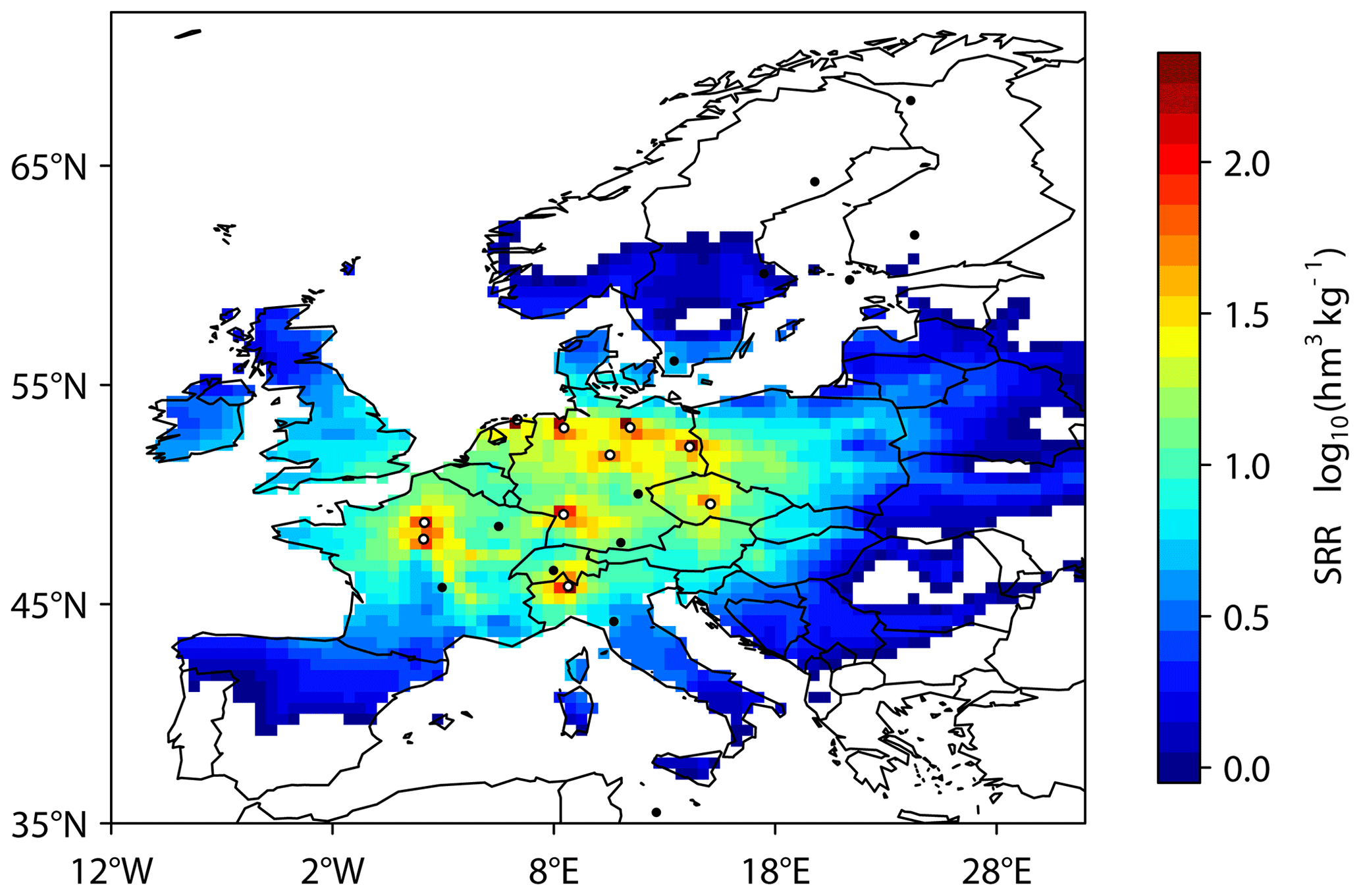
Figure 4 Map of the total mean SRR for optimal sites for monitoring fossil fuel CO₂ emissions with monthly resolution and including existing information from CO₂ mixing ratios. The locations of the optimal sites are indicated by the white points (i.e. SAC, KIT, LUT, KRE, STE, LIN, GAT, IPR, TRN, and TOH), and the locations of the unselected sites are indicated by the black points.

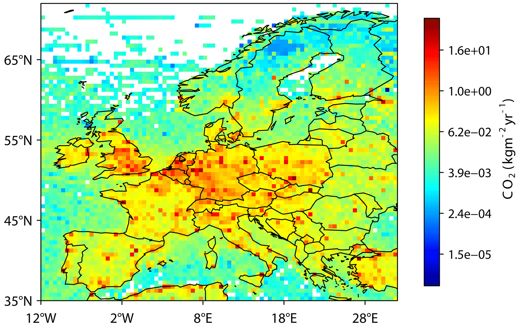
Figure 5 Map of annual mean fossil fuel CO₂ emissions (units of kg m⁻² yr⁻¹) plotted with a logarithmic (base of 2) colour scale.

4 Discussion

An obvious question is how does the criterion of information content compare to criteria based on the posterior uncertainty? The information content describes the change in probability space from before an observation is made (prior probability) compared to after an observation is made (posterior probability) and is thus more closely linked to the observations themselves than to the exact definition of the posterior uncertainty metric. The performance of the two metrics, i.e. information content versus the sum of the posterior error covariance matrix, was examined using the CH₄ example in scenario 1 (described in Sect. 3.1). For this example, a second network was selected using the criterion of the sum of the posterior error covariance matrix and consisted of the sites HPB, HTM, KRE, PUY, and TRN (only KRE was also selected using the information criterion). Two inversions were performed using pseudo-observations generated by applying the transport operator, H (with rows corresponding to daily afternoon means for each site and columns corresponding to the six source types resolved annually), to the annual mean fluxes for each source type, x, and adding random noise according to the error characteristics of R.

$$\begin{array}{}\text{(26)}& {\mathit{y}}_{\mathrm{obs}}=\mathbf{H}\mathit{x}+{\mathbf{R}}^{\frac{\mathrm{1}}{\mathrm{2}}}r\mathrm{where}r\sim N\left(\mathrm{0},\mathrm{1}\right)\end{array}$$

In these inversions, the prior was generated by randomly perturbing the fluxes according to the error characteristics of B.

$$\begin{array}{}\text{(27)}& {\mathit{x}}_{\mathrm{b}}=\mathit{x}+{\mathbf{B}}^{\frac{\mathrm{1}}{\mathrm{2}}}r\mathrm{where}r\sim N\left(\mathrm{0},\mathrm{1}\right)\end{array}$$

Both inversions used the same prior fluxes and uncertainties and differed only in the set of sites used. The performance of the inversions was tested using the so-called gain metric, G, based on the ratio of the distance of the posterior from the true fluxes to the distance of the prior from the true fluxes:

$$\begin{array}{}\text{(28)}& G=\mathrm{1}-\sqrt{{\displaystyle \frac{{\left(\mathit{x}-{\mathit{x}}_{\mathrm{a}}\right)}^{\mathrm{2}}}{{\left(\mathit{x}-{\mathit{x}}_{\mathrm{b}}\right)}^{\mathrm{2}}}}},\end{array}$$

where x_a is the posterior flux vector. The larger the value of G, the closer the posterior is to the true flux. Using the optimal sites according to the information content G=0.6996, while using the optimal sites according to the posterior error covariance G=0.6988. (A comparison of the prior and posterior compared to the true fluxes is shown in Fig. 6.) Thus, the information content performs at least as well as the posterior error covariance metric for determining a network.

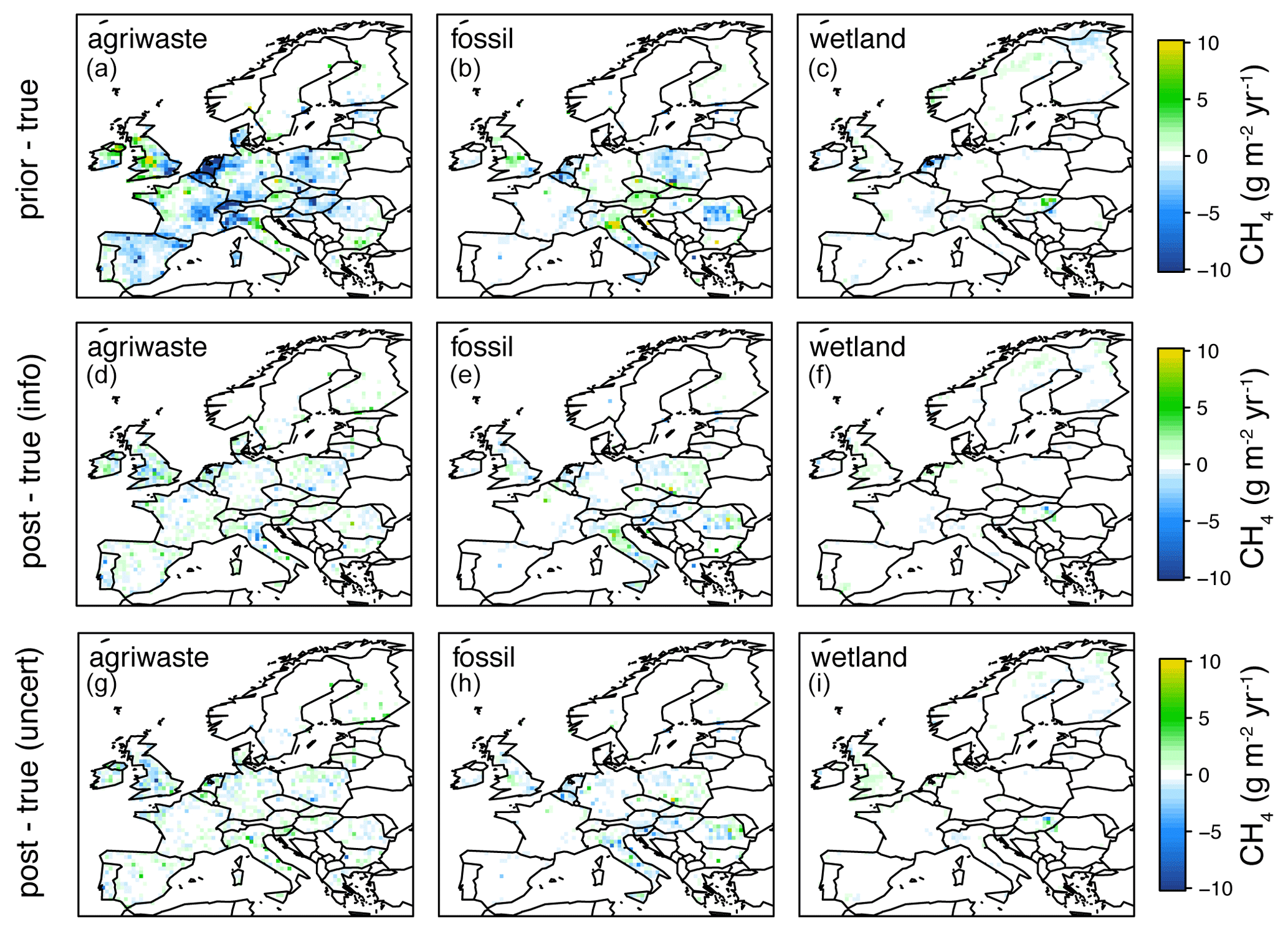
Figure 6 Comparison of the true-prior flux differences (units g m⁻² yr⁻¹) (a–c) versus the true-posterior flux differences for the inversion using sites chosen with the information content criterion (d–f) and the inversion using sites chosen with the posterior uncertainty criterion (g–i). Note: only the fluxes for the sources agriculture and waste, fossil, and biomass burning sources are shown as the other three sources are very minor.

Another question that arises is how does this method compare to methods based on the analysis of the variability in the time series at the different sites? To answer this question, a clustering method was applied to the example of designing a network for fossil fuel CO₂ emissions. For this, a time series of Δ¹⁴CO₂ was generated for each of the 24 sites using Eq. (25) (see the Supplement for plots of the time series). The values were generated hourly, but, since generally only daytime values are used in inverse modelling, data were selected for the time interval 12:00 to 15:00 LT​​​​​​​. A dissimilarity matrix was calculated for the 24 time series (using the R function proxy::dist with the dynamic time warp (DTW) method; Giorgino, 2009). The divisive hierarchical clustering method (R function cluster::diana) was applied to the dissimilarity matrix, stopping at 10 clusters. The first cluster contained 13 sites, that is, those with little signal (e.g. JFJ, CMN, and ZEP). Two clusters contained two sites, namely IPR and KRE, as well as OPE and TRN, while the remaining clusters contained only one site. Based on the principle of choosing sites that display different signals, one would choose the sites which are in a cluster of one. This would lead to the choice of GAT, KIT, LIN, LUT, SAC, STE, and TOH. These seven sites are also chosen by the method based on information content. However, the question is how to choose the remaining three sites from clusters with more than one site. For this there is no single answer. Moreover, the sites that are the most dissimilar are not necessarily those that will provide the most information about the target fluxes of the network, since the reasons for dissimilarity are various, e.g. having little signal, being sensitive to sources that are not the target of the network, or owing to distinct atmospheric circulation patterns. Sites with high degrees of similarity may both offer a strong constraint and both be valuable to a network (in this example IPR and KRE were in the same cluster, but both sites are chosen in the method based on information content).

In the examples presented, the atmospheric transport matrix, H, and the matrix, B, were resolved at 0.5^∘ × 0.5^∘ (and considered only land grid cells) and monthly. The size of the matrix B (and the matrix ${\mathbf{H}}^{\mathrm{T}}{\mathbf{R}}^{-\mathrm{1}}\mathbf{H}+{\mathbf{B}}^{-\mathrm{1}}$) for the example of a network for fossil fuel CO₂ emissions was ∼ 11  Gb. However, in the case of finer spatial resolution or a larger domain, which means the size of the matrices exceeds the available memory, it is still possible to use this method as long as B and ${\mathbf{H}}^{\mathrm{T}}{\mathbf{R}}^{-\mathrm{1}}\mathbf{H}+{\mathbf{B}}^{-\mathrm{1}}$ defined for one time step do not exceed the memory. In this case, the problem can be solved by summing the information content calculated separately for each time step. Disaggregating the problem in this way does not lead to the same value of information content as when all time steps are considered together; however, the choice of sites is nearly the same. For the example of a network for fossil fuel CO₂ emissions, the two methods (i.e. disaggregating versus not disaggregating) differed by only one site. For the example of a fossil fuel network, the total computation time was ∼ 3 h using multi-threaded parallelization on eight cores.

In addition to the memory requirements, there is the question of the computational cost determined by the complexity of the algorithm, in particular compared to the more established method using a metric based on the posterior error covariance. Such analysis can be performed putting aside the practical considerations related to particular software and/or hardware. It has been established that the algorithmic complexity, and hence the computational cost, of the calculation of the determinant is the same as that of matrix multiplication (Strassen, 1969; Aho et al., 1974). Ignoring the particularities of the algorithm used and its hardware implementation, the analysis can be simplified by counting the number of matrix multiplications: O(mnk) for two generic rectangular matrices, Cholesky decompositions ($O\left(n^{\mathrm{3}}\right)/\mathrm{3}$), matrix inversions, and determinant calculations (both obtained e.g. from the Cholesky decomposition). Both the error covariance metric and the information metric require the inversion of the matrix B. The covariance metric requires the Hessian matrix $\mathbf{G}={\mathbf{H}}^{\mathrm{T}}{\mathbf{R}}^{-\mathrm{1}}\mathbf{H}+{\mathbf{B}}^{-\mathrm{1}}$that takes one inversion of B ($\sim O\left(n^{\mathrm{3}}\right)/\mathrm{3}$), one inversion of R ($\sim O\left(k^{\mathrm{3}}\right)/\mathrm{3}$), and the product of three matrices ($O(n{k}^{\mathrm{2}}+n^{\mathrm{2}}k)\sim O\left(n^{\mathrm{2}}\right)$ if k≪n). This yields G in $O\left(n^{\mathrm{3}}\right)/\mathrm{3}+O\left(k^{\mathrm{3}}\right)/\mathrm{3}+O(n{k}^{\mathrm{2}}+n^{\mathrm{2}}k)$ operations. The inverse of G yields the posterior covariance in $O\left(k^{\mathrm{3}}\right)/\mathrm{3}$ operations via the Cholesky decomposition. Subsequent steps are of lower computational order. Even if some simplifications are possible, its complexity is bounded below by $\mathrm{2}O\left(n^{\mathrm{3}}\right)/\mathrm{3}$. Therefore, the information metric is not computationally more expensive than the covariance metric. The algorithm presented here is faster than the naive computation of the information content from its formal definition.

5 Conclusions

A method for designing atmospheric observation networks is presented based on information theory. This method can be applied to any type of atmospheric data: mixing ratios, aerosols, isotopic ratios, and total column measurements. In addition, the method allows the network to be designed with or without considering existing information, which may also be of a different type, e.g. mixing ratios of a different species or isotopic ratios. Since the method does not require inverting any large matrices (e.g. for the calculation of posterior uncertainties), and the calculation of B⁻¹ only needs to be performed once, it is very efficient and can also be used on large problems. The only constraint is that the matrices B and H^TR⁻¹H + B⁻¹ defined for one time step do not exceed the available memory. The algorithm allows the exact problem to be defined, that is, to target specific emission sources or regions. Two examples are presented: the first is to select sites from an existing network of CH₄ mixing ratios for additional measurements of δ¹³C to constrain emissions in EU countries (plus Norway, Switzerland, and the UK), and the second is to select sites from an existing network of CO₂ mixing ratios for additional measurements of Δ¹⁴CO₂ to monitor fossil fuel CO₂ emissions. These examples demonstrated that the optimal network differs depending on its exact purpose, e.g. is the network targeting emissions over the whole domain or for a specific region? And should existing information be considered or not? Thus it is important that the method of network design is able to account for these considerations.