the Creative Commons Attribution 4.0 License.
the Creative Commons Attribution 4.0 License.
 | 25 May 2023
The Far-Infrared Radiation Mobile Observation System (FIRMOS) for spectral characterization of the atmospheric emission
Flavio Barbara
Marco Barucci
Giovanni Bianchini
Francesco D'Amato
Samuele Del Bianco
Gianluca Di Natale
Marco Gai
Alessio Montori
Filippo Pratesi
Markus Rettinger
Christian Rolf
Ralf Sussmann
Thomas Trickl
Silvia Viciani
Hannes Vogelmann
Luca Palchetti
The Far-Infrared Radiation Mobile Observation System (FIRMOS) is a Fourier transform spectroradiometer developed to support the Far-infrared Outgoing Radiation Understanding and Monitoring (FORUM) satellite mission by validating measurement methods and instrument design concepts, both in the laboratory and in field campaigns. FIRMOS is capable of measuring the downwelling spectral radiance emitted by the atmosphere in the spectral band from 100 to 1000 cm−1 (10–100 µm in wavelength), with a maximum spectral resolution of 0.25 cm−1. We describe the instrument design and its characterization and discuss the geophysical products obtained by inverting the atmospheric spectral radiance measured during a campaign from the high-altitude location of Mount Zugspitze in Germany, beside the Extended-range Atmospheric Emitted Radiance Interferometer (E-AERI), which is permanently installed at the site. Following the selection of clear-sky scenes, using a specific algorithm, the water vapour and temperature profiles were retrieved from the FIRMOS spectra by applying the Kyoto protocol and Informed Management of the Adaptation (KLIMA) code. The profiles were found in very good agreement with those provided by radiosondes and by the Raman lidar operating from the Zugspitze Schneefernerhaus station. In addition, the retrieval products were validated by comparing the retrieved integrated water vapour values with those obtained from the E-AERI spectra.
- Article
(7212 KB) - Full-text XML
- BibTeX
- EndNote


The far-infrared (FIR) portion of the Earth's emission spectrum is the subject of a growing research interest because of its important role played in the Earth's radiative balance. This spectral region covers the wavelengths longer than 15 µm (the wavenumbers below 667 cm−1) and is strongly characterized by the pure rotational absorption band of water vapour and the ν2 carbon dioxide band. Several atmospheric and surface processes contribute to both the outgoing and the incoming radiation at these wavelengths in a complex and entangled manner (for a detailed discussion, see Harries et al., 2008; Palchetti et al., 2020b). In this context, spectrally resolved radiometric observations are a valuable tool that can potentially quantify the role of each of these contributions to the overall radiative balance.
To date, the FIR component of the outgoing longwave radiation has only been measured a few times during balloon campaigns by REFIR-PAD (Palchetti et al., 2006) and FIRST (Mlynczak and Johnson, 2006) and by the airborne instrument TAFTS (Cox et al., 2010). On the other hand, several ground-based experiments observed the FIR portion of the downwelling longwave radiation (DLR): the Earth Cooling by Water Vapor Radiation (ECOWAR) experiment (Bhawar et al., 2008) and the Radiative Heating in Underexplored Bands Campaigns (RHUBC-I and RHUBC-II; Turner and Mlawer, 2010; Turner et al., 2012). Eventually, REFIR-PAD was installed in Antarctica at the Concordia station, where it has been in continuous operation since 2011 (Bianchini et al., 2019).
FIR spectral measurements of DLR proved valuable for refining the knowledge of water vapour spectroscopy (Mlawer et al., 2019) and testing the ability to model radiative transfer in the atmosphere (Mlynczak et al., 2016; Mast et al., 2017; Bellisario et al., 2019; Mlawer et al., 2019). In addition, ground-based FIR observations were successfully exploited to infer cloud properties (Maestri et al., 2014; Rizzi et al., 2016; Di Natale et al., 2017), to retrieve the thermal structure and composition of the atmosphere (Rizzi et al., 2018; Bianchini et al., 2019), and to conduct radiative closure studies (Delamere et al., 2010; Sussmann et al., 2016).
The Far-infrared Outgoing Radiation Understanding and Monitoring (Palchetti et al., 2020b, FORUM) project has been selected as the 9th European Space Agency's Earth Explorer Mission, to be launched in 2027. The FORUM core instrument will be a Fourier transform spectrometer (FTS), and it will measure the Earth's upwelling spectral radiance from 100 to 1600 cm−1 (100–6.25 µm). FORUM will allow for the first time to observe globally the Earth's spectrally resolved emission in the FIR.
During the preparatory phase of FORUM, the Far-Infrared Radiation Mobile Observation System (FIRMOS) was employed to support the mission by validating measurement methods and instrument design concepts, both in the laboratory and in field campaigns. Throughout this activity, the data gathered have been critically employed for the validation of geophysical parameters, retrieval codes, and more generally to expand FIR spectroscopic knowledge.
FIRMOS was built at the Italian National Institute of Optics of the National Research Council (INO-CNR), and it was designed as a laboratory and field campaign flexible instrument. Subsequently it was deployed in the German Alps at the summit station of the Zugspitze Observatory (2962 m a.m.s.l.) for a 2-month campaign (Palchetti et al., 2021) in winter 2018–2019. Some of the measurements collected during that time are presented here to demonstrate the capabilities of the platform. During the campaign at Zugspitze, FIRMOS was jointly operated with an assortment of co-located instruments that characterized the observed atmospheric state. The spectra acquired during the campaign were processed to derive higher level products, namely temperature and water vapour profiles and cloud properties, if applicable.
In this paper, we describe the instrument design and its characterization, and we discuss the temperature and water vapour products obtained by inverting the atmospheric spectral radiance measured during the campaign in clear-sky conditions. The retrieval of optical and microphysical cloud properties is the subject of a separate publication (Di Natale et al., 2021). Section 2 introduces and describes in detail the FIRMOS instrument, its optomechanic design, radiometric calibration, electronics, and detection specifics; Sect. 3 presents the Level 1 (L1) and Level 2 (L2) data, while in Sect. 4 the results are discussed. Finally, in Sect. 5 the conclusions are drawn.
FIRMOS was designed and built first as a laboratory prototype and was successively adapted to obtain a versatile instrument that could be quickly deployed in ground-based field campaigns (<80 kg, 1 d readiness), specifically at high altitude sites and easily adaptable to stratospheric balloon flights.
The instrument was built during the compressed schedule preceding the Earth Explorer 9 mission selection and deployed for its first campaign at the Zugspitze Observatory in the Bavarian Alps (South Germany; 47.421∘ N, 10.986∘ E, 2962 m a.m.s.l; Palchetti et al., 2021) between the end of 2018 and the beginning of 2019. FIRMOS mostly acquired atmospheric DLR spectra, in zenith-viewing configuration; at the end of the campaign, some days were allocated to surface-looking measurements of a variety of snow samples.
Table 1Characteristics of the measurements performed at Zugspitze during the FIRMOS campaign (Palchetti et al., 2021).
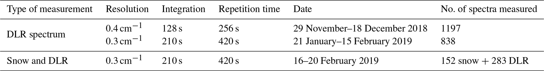
A set of instruments was operated in conjunction with FIRMOS: E-AERI, an IR commercial FTS at the Zugspitze summit; a lidar instrument at the Schneefernerhaus station (UFS) at 2675 m a.m.s.l., 700 m to the south-west of the summit station; and five dedicated radiosonde launches were carried out from Garmisch–Partenkirchen, 8.6 km to the north-east of the summit. More details are given within the sections below.
2.1 The FIRMOS instrument
FIRMOS is a ground-based FTS operating in the far- and mid-infrared range. Its design stems from its predecessor, the Radiation Explorer in the Far InfraRed – Prototype for Applications and Development (Bianchini et al., 2019, REFIR-PAD). The new design, as described in the following sections, is the result of a rationalization aimed at a leaner instrumental setup and at reducing deployment times by employing commercial parts for motion control and reflective optics.
2.1.1 Optomechanics
The optical layout of the FIRMOS interferometer is composed by double-input and double-output Mach–Zehnder configuration. The setup allows full tilt compensation by employing a movable unit with roof-top mirrors (RTMU). Additional flat mirrors are used on the right arm of the interferometer to compensate for slit yaw. Parabolic mirrors (45∘ off axis) enable light focusing on the detectors, encapsulated with caesium iodide windows. The reference source is a 785.9 nm single-mode thermally stabilised laser (Thorlabs). The latter is driven with a constant current from a controller developed in-house and already employed within the previous REFIR-PAD instrument. The reference laser follows the same optical path as the infrared beam, with dedicated optics joined to the same mountings as for the main measurement.
Radiometric accuracy is achieved by employing three blackbody sources, the hot (HBB) and the cold (CBB) calibration blackbodies, and the reference blackbody (RBB). A rotating mirror (PM0) located at the interferometer first input can select either the HBB, the CBB, or the sample scene (Fig. 1); the contribution of this mirror to the instrument response is therefore accounted for in the calibration procedure (see Sect. 2.1.3). The RBB, located at the second input, is in thermal equilibrium with the other optical components. At every measurement cycle, the calibration procedure is performed before and after the sample scene.
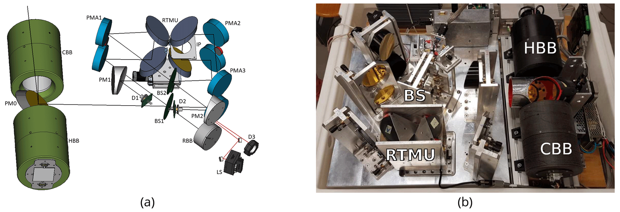
Figure 1FIRMOS: (a) optical layout diagram, the blackbodies (HBB and CBB) are depicted in green, PM0 indicates the scene selection mirror. The roof-top mirrors unit (RTMU) is on the top right, IP is the internal pupil, in the centre BS1 and BS2 indicate the beam splitters. The whole optical path is folded on two levels using mirrors (PMA1, PMA2, PMA3, PM1, PM2). Also shown are the pyroelectric detectors (D1 and D2), the reference laser (LS) and its detector (D3), and the reference (RBB) (b) picture of the inner structure of the instrument.
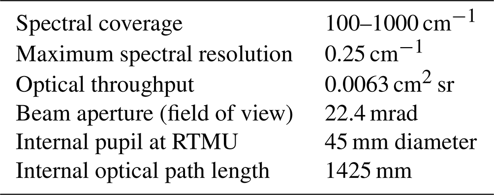
The FIRMOS setup was designed to maximize the optical throughput by employing 76.2 mm diameter optics while maintaining a field of view of 22 mrad. In addition, the optical system is image forming at the detector, although the latter is a single pixel (diameter of 2 mm). The above features are meant to enhance the observed scene selectivity while maintaining good signal-to-noise ratio, and therefore to facilitate the development of software tools for geophysical parameters retrieval.
The field of view in FIRMOS is defined by the optical path length of the instrument, the internal pupil radius, and the detector area, the latter being the main limiting factor in the current design. The optical specifications of the instrument are listed in Table 2.
To cover the IR spectral range from 100 to 1000 cm−1, the instrument adopts wideband germanium-coated biaxially-oriented polyethylene terephthalate (BoPET) beam splitters (BS) and room temperature deuterated L-alanine doped triglycene sulfate (DLATGS) pyroelectric detectors. The absorption of the BoPET BS substrate causes some degradation in efficiency in some narrow bands around 730, 850, 873, and 973 cm−1, as can be seen in Fig. 2 which shows the typical 4RT efficiency. The instrument spectral range is limited at low wavenumbers by the absorbance of the detector CsI windows and at high wavenumbers by degradation of the optical performance due to BSs flatness errors (see Figs. 2b and 8).

Figure 2(a) Interferometric efficiency of the beam splitter. (b) Interferometric image of a beam splitter sample.
The BS samples were manufactured at INO-CNR and tested with a Newton interferometer, to select those with maximum flatness. The interferometer is capable of detecting flatness anomalies with 0.1 µm precision by employing a reference surface with a flatness of , a monochromatic source, and a digital camera. The pattern observed in the case of membranes with a divergence from flatness of a few micrometres is of the saddle or multi-saddle type, especially close to the edge. The saddle peak-valley distance is evaluated through the measurements of the number of fringes on the main saddle along a track (Fig. 2b). The best two BS samples, with flatness error of less than 2.5 µm peak-valley, were integrated on FIRMOS to guarantee good performance over the 100–1000 cm−1 range.
A lightweight and compact linear stage model (Zaber model X-LSM025A; mass: <0.5 kg, height: 20 mm, centred load capacity: 100 N) was used, installed within a notch of the breadboard below the RTMU to perform the interferometric scan. A scanning speed of 0.25 mm s−1 in a 30–60 s acquisition time for a single scan is used. The typical standard deviation of speed over a scan was obtained experimentally as 0.043 mm s−1 at a 0.25 mm s−1 scan speed, sufficiently stable to be accounted for during the signal analysis.
The RTMU was manufactured from a monolithic aluminium piece (see Fig. 1b). The mirrors are placed in a roof-top configuration and fixed by a system of springs and screws.
The instrument was designed for easy transportation and deployment. Its size is cm, it weighs 80 kg, and the power consumption is 60 W. A plastic enclosure was used to protect against environmental conditions, an 8 cm diameter aperture with a motorized shutter was used for observation.
The instrument breadboard was realized as a monolithic aluminium slab with a mass of 17.5 kg and dimension of mm (). Rods spacing and tightening points were initially designed balancing dimensions, mass, and stiffness of the framework. The final layout was identified through an iterative design process carried out with CAD software that evaluated static loads.
2.1.2 Radiometric calibration unit
In order to perform a calibrated radiometric measurement, at least two known radiation sources are required. In FIRMOS the HBB and a CBB are located at the instrument entrance. The scene mirror allows the acquisition of the external view of the instrument (zenith or nadir) or one of the two BBs. The axial rotation is obtained through a stepper motor (NEMA 17 stepper), that also supports the mirror, surrounded by a plastic guard in order to prevent stray light from other instrument components. The support was assembled out of 3D-printed high strength co-polyester plastic parts.
Monte Carlo numerical calculations were performed to optimize the cavity geometry of the BBs, in order to maximize normal emissivity, a 34∘ angle was chosen for both the HBB and CBB inner cones (see Fig. 3) achieving an emissivity >0.9985.
The CBB was assembled in a 3D-printed co-polyester plastic shell and the HBB was assembled in a 3D-printed heat-resistant carbon fibre-reinforced Nylon plastic shell, they were both designed to minimize thermal dispersion. The BBs cavities were fabricated in aluminium, internally coated using NEXTEL velvet coating 811-21. Some layers of thermal superinsulation foils were placed inside the plastic shells, in order to minimize the thermal exchange between the aluminium structure and its plastic supports.
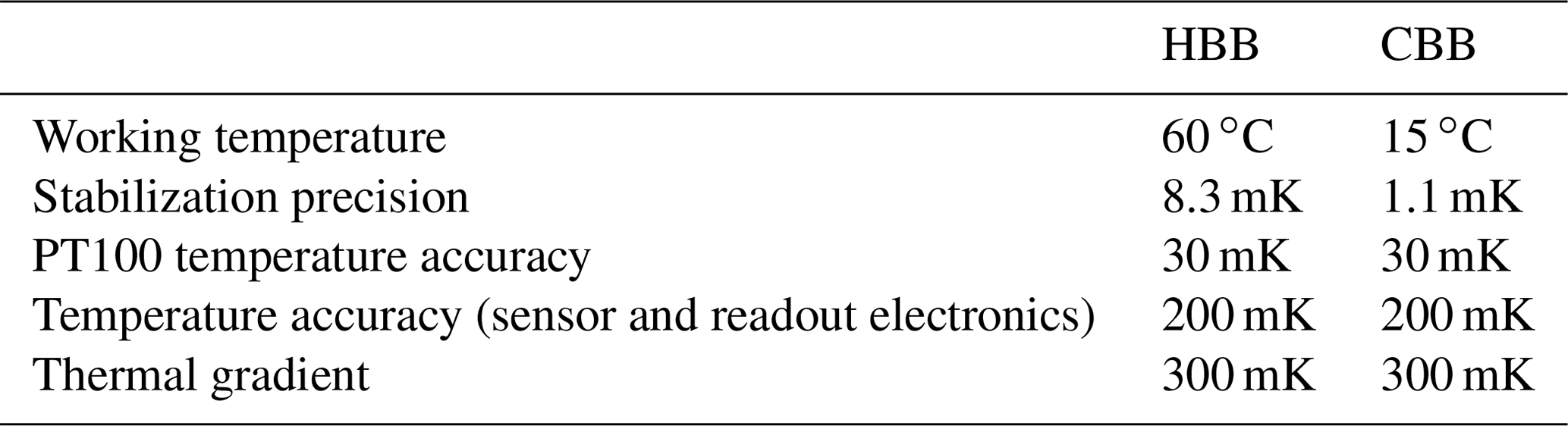
The BBs controllers are two modular drivers for temperature reading and stabilization, developed in-house. The temperature of the RBB is monitored by a supplementary module of the HBB driver. Each BB controller simultaneously records the temperature of four sensors: one high-accuracy (30 mK) resistance temperature detector (PT100 sensor) for the measurement of the BB temperature, one high-resolution (500 µK) negative temperature coefficient (NTC) sensor for active thermal stabilization, and two one-wire digital thermometers (Dallas DS18B20). The position of the sensors inside the BBs is shown in Fig. 3.

Due to the sensor high accuracy, the PT100 is employed to measure the BB temperature value used in the L1 data analysis. The PT100 temperature reading by the FIRMOS controller and by a commercial temperature monitor (Lakeshore; model 218, with a temperature equivalent accuracy of 68 mK) were compared to estimate the contribution of the readout electronics to the accuracy of the BB temperature. The comparison showed a maximum positive offset of 200 mK between the two, this value was conservatively assumed as the BB temperature total accuracy.
The NTC temperature is used for the thermal stabilization of the BB. Each stabilization controller is equipped with a proportional integral derivative (PID) circuitry to maintain the temperature read from the NTC, equal to a selected value. The HBB controller operates in heating-only mode by driving a heater resistor mounted inside the HBB. The CBB controller operates in cooling/heating mode by driving a Peltier element placed inside the CBB.
Two Dallas sensors, located at the opposite extremities of the BB, are used to monitor the BB thermal homogeneity.
For the field campaign, the CBB and the HBB were typically stabilized at a temperature of 15 and 60 ∘C, respectively. In order to find the precision of the BB thermal stabilization, the difference between the PT100 reading and the set point (the so-called temperature stabilization error) was recorded for some hours. Figure 4 shows the PT100 measurements after stabilization was activated, for the HBB (Fig. 4a) and the CBB (Fig. 4c). Figure 4b and d shows the temperature stabilization error after the set point is reached, respectively, for the HBB and the CBB. The HBB reached the temperature of 60 ∘C in approximately 2 h, and the CBB reached 15 ∘C in approximately 30 min. To infer the precision of the temperature stabilization, assumed as the standard deviation of the stabilization error after the set temperature is reached, we calculated the standard deviation of the signals reported in Fig. 4b and d. The HBB controller provides a stabilization precision of 8.3 mK, and the CBB controller provides a stabilization precision of 1.1 mK.
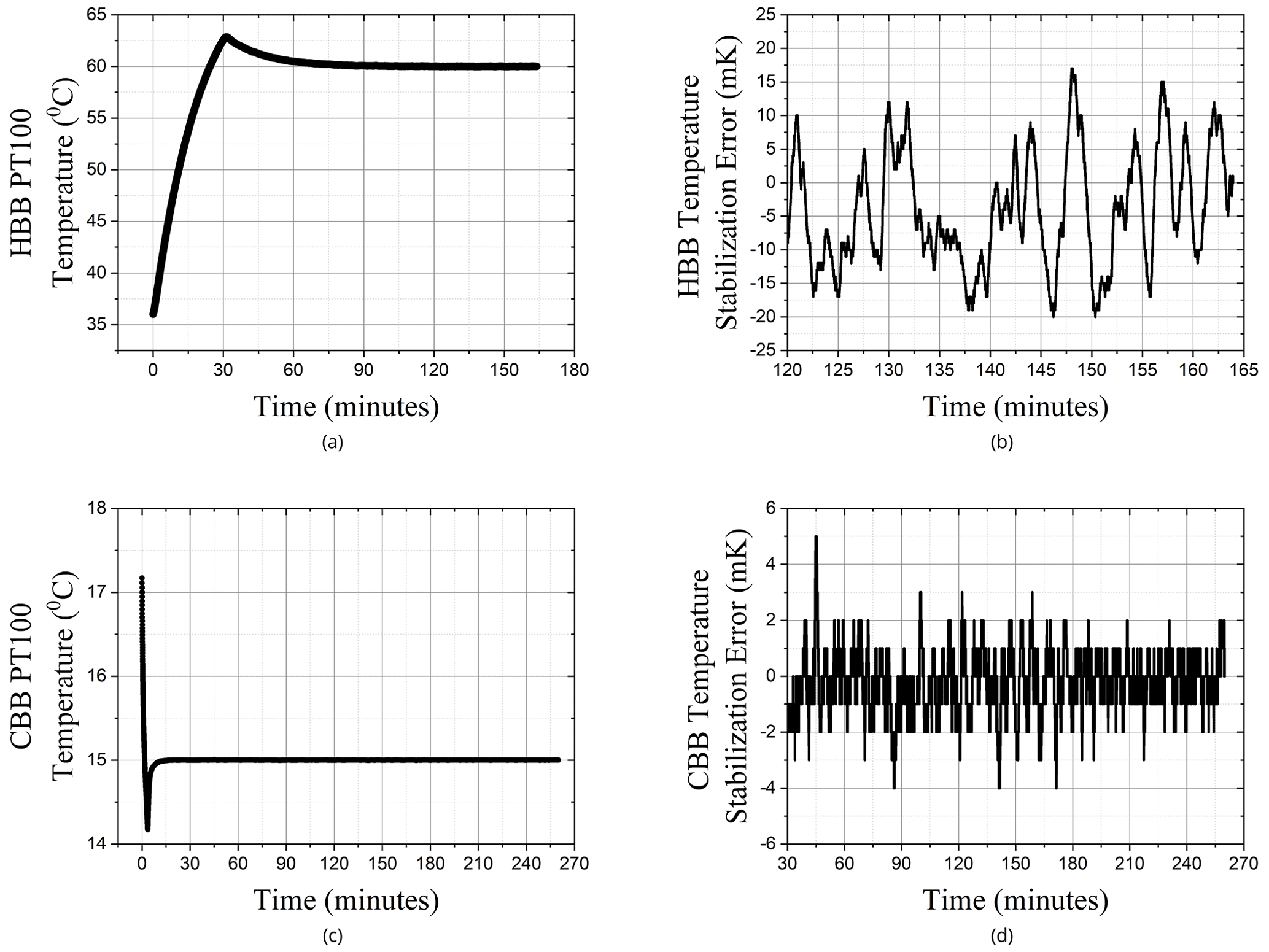
Figure 4(a) Time evolution of the PT100 temperature for the HBB since the stabilization controller is activated. (b) Difference between the HBB PT100 temperature and the target temperature (70 ∘C) after the thermal stabilization is reached. (c) Time evolution of the PT100 temperature for the CBB. (d) Difference between the CBB PT100 temperature and the target temperature (15 ∘C) after the thermal stabilization is reached.
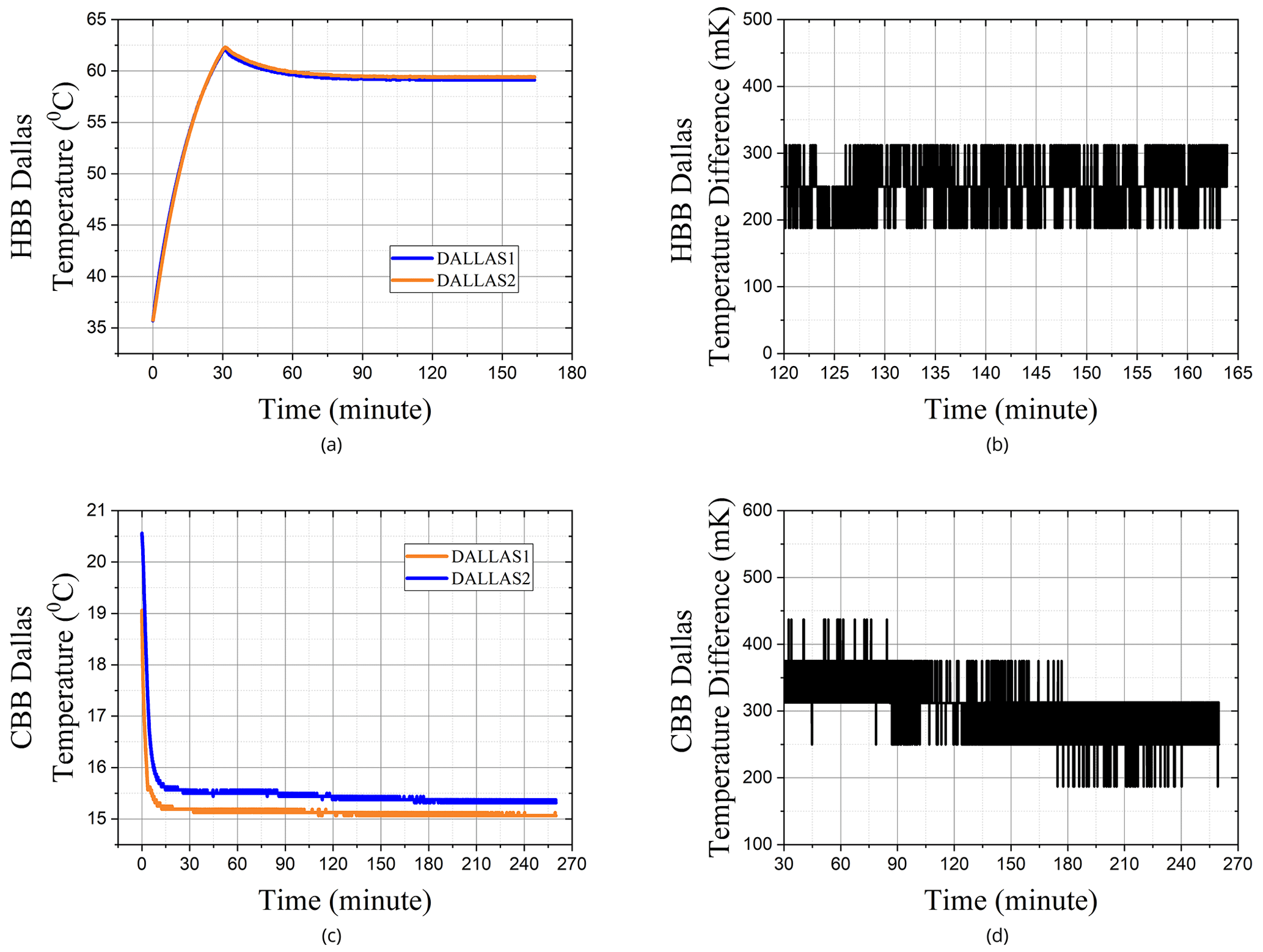
Figure 5(a) Time evolution of the Dallas1 (orange line) and Dallas2 (blue line) HBB sensors after the stabilization controller is activated (target temperature: 70 ∘C). (b) Temperature difference between the HBB Dallas sensors after the thermal stabilization is reached. (c) Time evolution of the Dallas1 (orange line) and Dallas2 (blue line) CBB sensors after the CBB stabilization controller is activated (target temperature: 15 ∘C). (d) Temperature difference between the CBB Dallas sensors after the thermal stabilization is reached.
The BBs temperature homogeneity was estimated from the time evolution of the difference between the readings of the two Dallas thermometers placed at the extremities of the BBs. Figure 5 shows the Dallas1 and Dallas2 measurements after stabilization was activated for the HBB (Fig. 5a) and the CBB (Fig. 5c), and the temperature difference between the two Dallas sensors after thermal stabilization was reached (Fig. 5b for the HBB and 5d for the CBB). After the set temperature was reached, the HBB Dallas thermal difference did not show a significant variation, and the thermal gradient remained constant with a mean value of 250 mK. The Dallas thermal difference for CBB showed only a slight decrease of about 30 mK h−1, and the mean value of the thermal gradient during 4 h resulted in 300 mK. The mean value of the temperature difference between Dallas2 and Dallas1, after temperature stabilization was reached, was assumed to be the thermal gradient of the BB. The BB thermal homogeneity was thus conservatively considered to be about 300 mK for both.
The BB controllers performance is summarized in Table 3.
2.1.3 Detectors and electronics
One of FIRMOS enabling technologies is the adoption of two room-temperature pyroelectric DLATGS detectors covering the mid-infrared and the far-infrared region. The detectors are uncooled (model: Selex P5180) and have a noise equivalent power NEP of 1.4 and W , where A and D* are, respectively, the detector area (3.14 mm2) and the detectivity. The pyroelectric preamplifiers were prepared at INO-CNR, and the electric scheme follows a classic design, previously tested for the REFIR-PAD instrument (Bianchini et al., 2019). The original scheme was optimized, miniaturizing as much as possible the amplifier to reduce the wiring length, in order to increase immunity to electromagnetic interference noise.
The slow response of pyroelectric detectors requires compensation for the acquired signals with digital processing in order to remove amplitude and phase distortions. For this purpose, the frequency response of the detector and of the pre-amplifier subsystem were characterized, measuring their frequency response to a laser-beam step excitation for both output channels (Fig. 6). An empirical model was successively derived from the measurements with a fitting procedure and then used to digitally compensate for the detector response during the L1a analysis (described in Sect. 3.1).
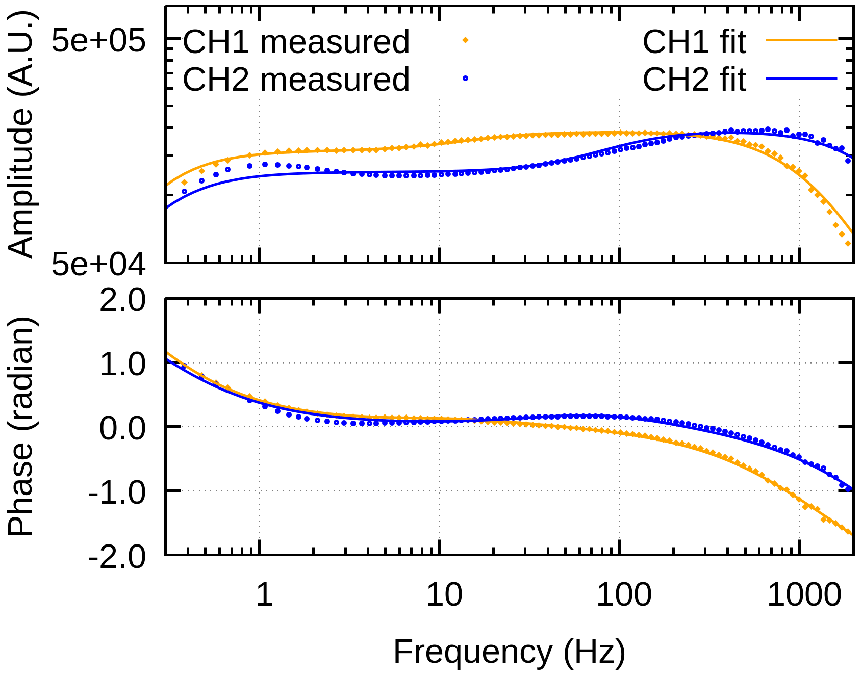
The FIRMOS detectors observe signal variations in the range of 5–100 Hz depending on the scanning conditions.
3.1 Level 1 data analysis (spectral calibration)
The L1 data analysis processes the interferograms acquired by the instrument to obtain calibrated spectra. The procedure follows the one described in more detail in Bianchini et al. (2008) for a double-input/double-output ports interferometer and is divided into three steps:
-
L1a performs the signal conditioning (filtering, detector response compensation, path-difference resampling, phase correction, etc.) and the Fourier transform;
-
L1b carries out the radiometric calibration providing the calibration functions and the calibrated spectra for each output channel;
-
L1c calculates the average spectrum for every measurement cycle, composed of sky observations and calibration measurements. L1c provides one average spectrum for each of the two output channels and the average of the two channels together with an estimate of the noise and the calibration error. All the averages are weighted by the respective noise estimate.
Each of the interferometer output signals is proportional to the difference of the two input signals with a wavenumber-dependent complex response function F, that is, in general, different for the two inputs and for the two output channels. As described above, the first input is used to measure the scene, whereas the second input, which corresponds to the instrument self-emission, looks continuously to the RBB source. Under these conditions, the relationship between the uncalibrated complex spectrum S(σ) and the calibrated spectrum of the observed scene L(σ), for each output channel, is given by the following:
where F1 and F2 are the calibration functions, and Br(σ) is the radiance from RBB, calculated from its measured temperature using the Planck law.
Calibration is carried out by changing the observed scene with the rotating mirror at the first input. The calibration functions F1 and F2 are obtained from a two-point radiometric calibration procedure, measuring sequentially the radiance of the HBB and CBB during each measurement cycle. The calibrated radiance spectrum L(σ) is then calculated from the uncalibrated spectrum S(σ) and the theoretical expression of Br(σ):
As noted in Bianchini et al. (2008), all the quantities used in the calibration procedure are complex; only in the last expression, Eq. (2), the real part of the result is taken, obtaining the measured spectrum as a real quantity. Furthermore, since the optical layout of the interferometer is equivalent with respect to the two inputs, F1 and F2 have almost the same values. Forward and reverse sweeps of the interferometer (optical path difference; and ) are treated separately during the calibration, since in general they will have different phase errors; nonetheless, the final spectral radiances can be averaged.
The precision of each measurement is calculated in terms of the noise equivalent spectral radiance (NESR) that has to be associated with the specific observation. This quantity depends on the number of acquisitions of the observed scene and the number of HBB/CBB calibration measurements during each measurement cycle, and it is dominated by the detector noise (random error component) ΔS, which is independent of the observed scene. The NESR is then obtained through error propagation of ΔS on the calibrated spectrum obtaining
where is the average of N scene acquisitions (four in FIRMOS standard acquisition configuration), and and are the averages of n HBB and CBB acquisitions (two in standard configuration), respectively. F1 and F2 are considered equal to F for the noise calculation. ΔS is obtained from the standard deviation of a series of uncalibrated measurements of a constant source, such as the CBB. The spectral dependence of all the variables in Eq. (3) is omitted for the sake of brevity.
Figure 7 reports the results for a typical observation of the atmosphere (NESR_atm) and of a reference blackbody source, measured inside the laboratory (NESR_bb). The NESR has sharp spectral features, where the noise increases, due to the absorption of the gases inside the interferometric path, mainly water vapour below 400 cm−1 and carbon dioxide at 667 cm−1, and the absorption bands of the BoPET BS, around 730, 850, 873, and 973 cm−1. Furthermore, the NESR estimate depends on the observed scene because of the error on the calibration source measurements that propagates on the NESR estimate through the calibration functions. If numerous calibration measurements are performed so that n is large enough to neglect the second term in Eq. (3) compared to , then the NESR estimate does not depend anymore on the observed scene and becomes an instrument specification (see NESR_instr curve in the bottom panel of Fig. 7). The latter approach is typically applied to specify the instrument performance in terms of the NESR, whereas the second term of Eq. (3) is accounted for in the calibration precision. However, in our case, we perform a calibration for each measurement cycle so that n is comparable with N; therefore, the total NESR estimate of Eq. (3) is a better estimate of the total random error of our single measurement.
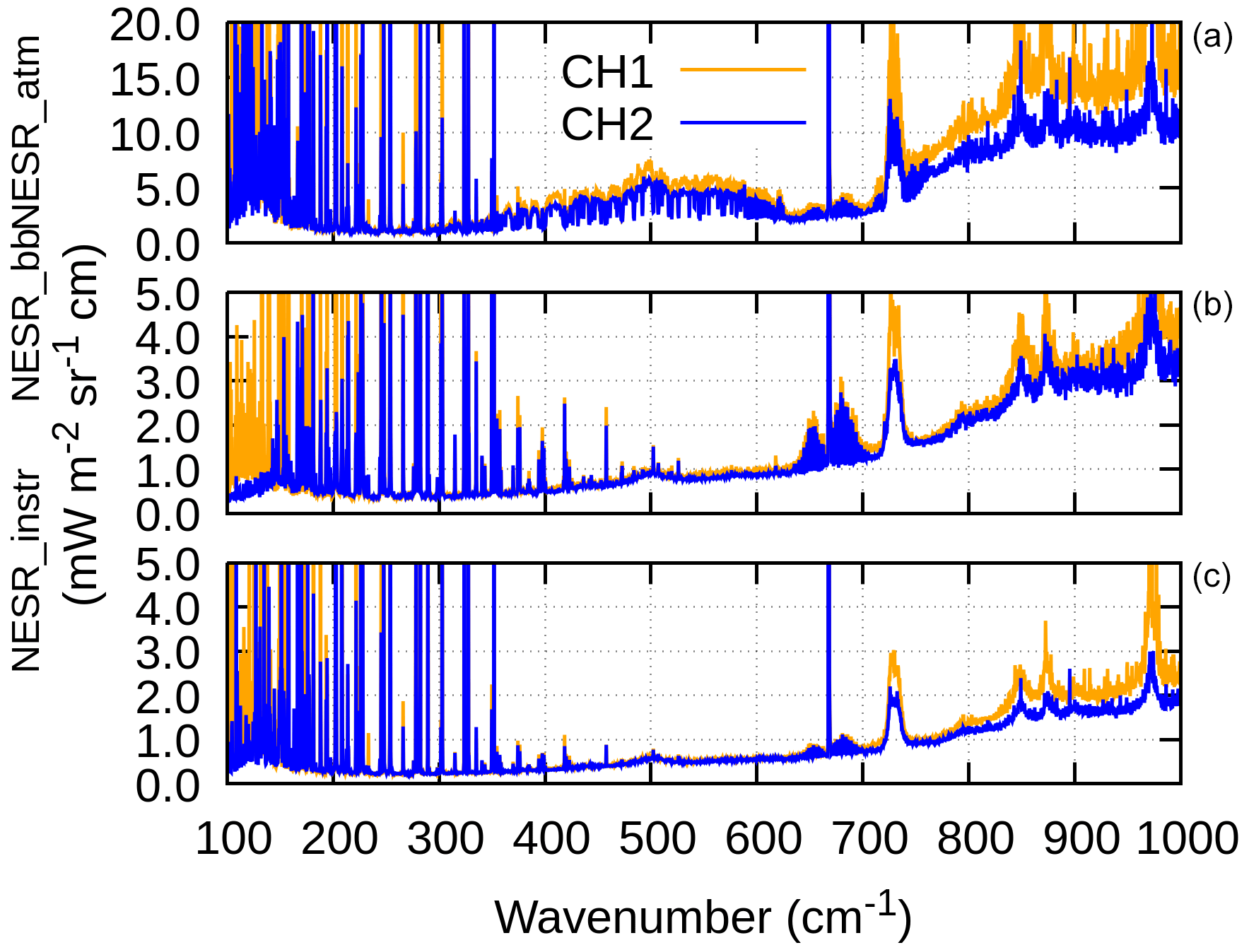
Figure 7NESR of the calibrated spectra calculated from error propagation of Eq. (3), in the case of a measurement cycle of N=4 sky measurements and n=2 for each calibration source. NESR_atm (a) is for the observation of the atmosphere in clear-sky condition, NESR_bb (b) is for the observation of a blackbody sources in laboratory, and NESR_instr (c) is the instrumental component equal to .
The increase of noise over 600 cm−1 in Fig. 7 indicates a performance degradation. Such degradation is mainly caused by the BS flatness error (see Fig. 2), as it can be inferred by Fig. 8 that shows the comparison of the measured NESR_instr (the same curves of the bottom panel of Fig. 7) with simulations carried out assuming a simple numerical model of the instrument NESR. The model includes the detector specifications and the optical efficiency of the interferometer, in the simulations the interfering wave fronts were distorted with a spherical shape to approximate the BS flatness error. The results of Fig. 8 demonstrate that measurements are consistent with a BS flatness error of about 2.2 µm in accordance with the results shown Fig. 2.
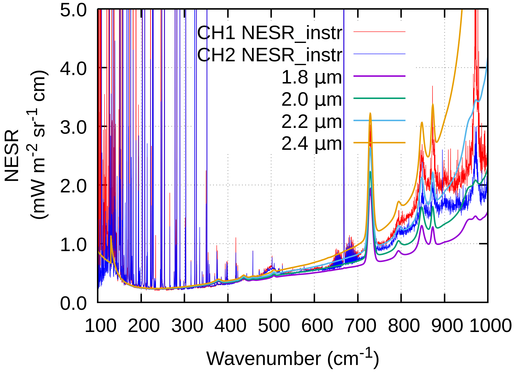
Figure 8Comparison of the measured NESR_instr (red and blue curves) with simulated NESR obtained with different values peak-valley of BS flatness errors shown in the legend.
The calibration error CalErr is spectrally correlated and can be calculated through the error propagation in Eq. (2) assuming as independent the uncertainty on the theoretical Planck emission of each BB (ΔBH, ΔBC, and ΔBR).
The uncertainty ΔBH, ΔBC, and ΔBR are dominated by the uncertainty of the temperature of the BB. The BB temperature error depends on two contributions: the accuracy of PT100 measurements and the BB thermal homogeneity. As the temperature accuracy is lower with respect to the thermal homogeneity, the temperature uncertainty for all BBs can be conservatively assumed to be equal to the thermal gradient of 300 mK. With this temperature error, the uncertainty due to the emissivity deviation from 1 gives a negligible contribution to the calibration error.
As shown in Fig. 9, the calibration error estimate also depends on the observed scenes and is larger for colder scenes when the sky is observed, since the uncalibrated signal S, which depends on the temperature difference between the observed scene and RBB (see Eq. 1), is larger in this case.
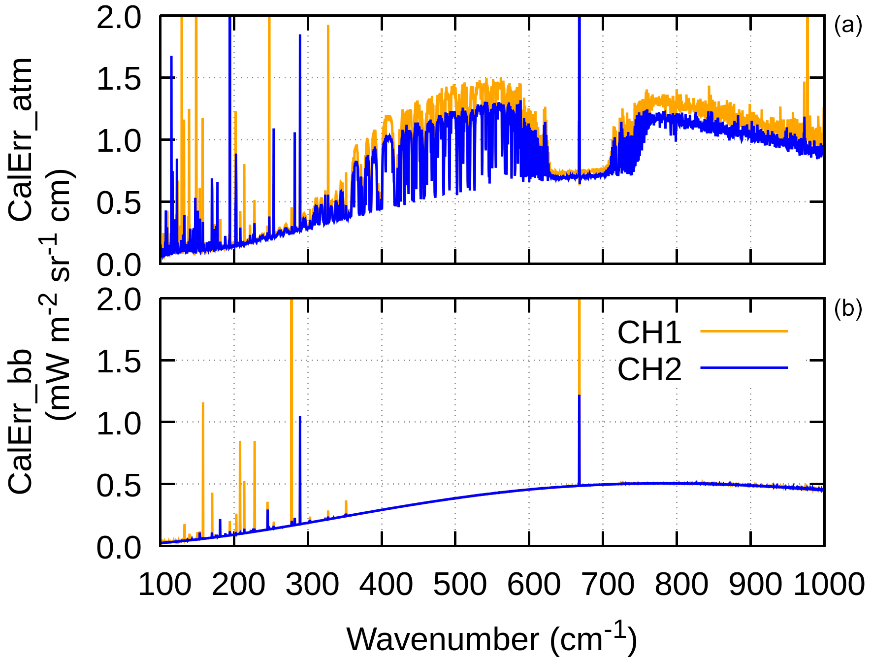
Figure 9Calibration error calculated from a conservative estimation of 0.3 K uncertainty on the temperature measurement of each reference blackbody. CalErr_atm (a) is for the observation of the atmosphere in clear-sky condition, CalErr_bb (b) is for the observation of a blackbody source in laboratory.
Finally, Fig. 10 shows an example of the spectrum and error estimates obtained as a weighted mean of the two channels after the L1c analysis. The measurement was acquired in clear-sky conditions during the campaign at Mount Zugspitze in measurement cycles, each comprised of four sky and four calibration observations, as described above. The total sky observation has a duration of 215 s, and the total measurement cycle time is 8 min. The standard deviation (SD in the figure) of the measurement, which is in good agreement with the NESR estimate used in the mean, is also shown in the figure.
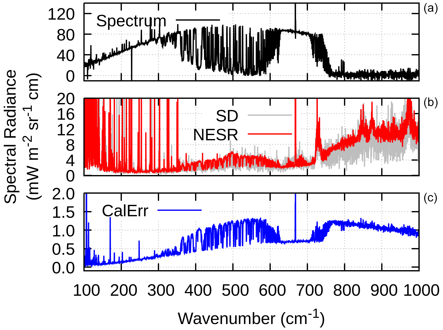
Figure 10Calibrated spectrum (a) and error estimates (NESR and SD (b)). Calibration error (c) obtained from the weighted mean of the two output channels in a measurement cycle of four zenith observations in clear-sky conditions on 25 January 2019 at 15:55 UTC.
3.2 Level 2 data analysis (retrieval)
FIRMOS L1 measurements were processed using the Kyoto protocol and Informed Management of the Adaptation (KLIMA) forward and retrieval models (Sgheri et al., 2022; Ridolfi et al., 2020; Del Bianco et al., 2013; Bianchini et al., 2008; Carli et al., 2007) to derive geophysical products (L2). Only spectra acquired from the instrument channel one were used since the second channel occasionally showed a degradation that could have a negative impact on the results. The retrieval of water vapour and temperature profiles was carried out on the entire clear-sky L1 dataset (as defined in Sect. 3.3), in the range of 200 to 1000 cm−1. The targets were retrieved from the surface up to 7 km on seven atmospheric layers for temperature and six for water vapour.
The algorithm uses an optimal estimation approach (Rodgers, 2004) and a multi-target retrieval strategy (Carlotti et al., 2006). Profiles from the National Centers for Environmental Prediction (NCEP) reanalysis (Kanamitsu et al., 2002) were used as initial guess and a priori. The a priori errors for temperature and water vapour were set to 0.3 % and 50 % of the averaged a priori values, respectively. The a priori covariance matrix was constructed assuming for both parameters a correlation length equal to 2 km between adjacent levels, while no cross-correlation was imposed between temperature and humidity.
3.3 Clear-sky selection criteria
The KLIMA model can analyse pure clear-sky scenes and scenes with optically very thin clouds; for this reason a subset of measurements not significantly perturbed by clouds in the FIRMOS band was first selected. The subset is referred to as the clear-sky cases subset.
Clear-sky cases were selected by evaluating the transparency and slope (gradient) of the FIRMOS spectra in the atmospheric window (AW; 820–980 cm−1). In the absence of clouds, the spectrum in the AW is well known and equal to the contribution of the water vapour continuum, which is small in comparison to the measurement noise. Likewise, an ideal noise-free and cloud-free measurement would have a gradient of 0 in the very dry winter conditions at Zugspitze, whereas negative values would correspond to a noise-free cloudy observation with a magnitude depending on the specific cloud.
The transparency of the AW was assessed in the narrow spectral window between 829 and 839 cm−1 by calculating the spectral average of the ratio of the signal with respect to the total noise as follows:
where ν1 and ν2 are the extremes of the AW spectral range, S is the measured spectral radiance and the quadratic sum of NESR, and the calibration error constitutes the total noise. The absolute value of Δ for a clear-sky observation is expected to be less than one, indicating that the measured signal is only due to noise fluctuations.
The slope was calculated between 786 and 961 cm−1 in six specific microwindows where gas absorption lines are absent: (786–790, 830–835, 856–863, 893–905, 912–918, 960–961 cm−1). The microwindows were selected from a spectrum simulated by the KLIMA forward model; the gradient was obtained from a linear fit of radiance on the microwindows. The fitted slope lies within the range . The maximum positive values, up to , are not physically consistent, and they can be related to noise fluctuations around zero.
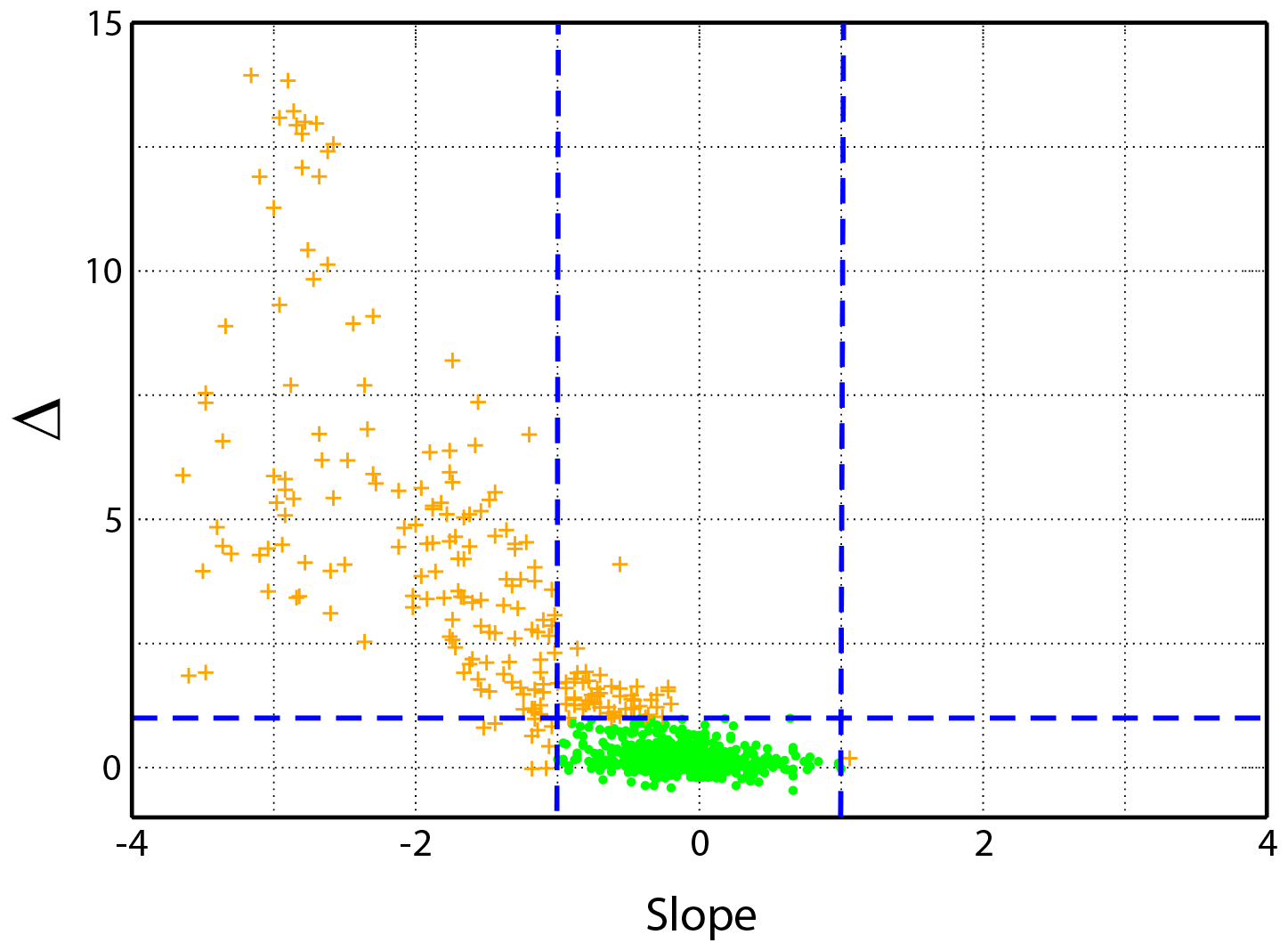
Figure 11Plot of the Δ ratio, as defined in Eq. (5), versus the normalized slope calculated using the six microwindows in the spectral range 786–961 cm−1 defined in the text. Dashed blue lines indicate the acceptance values, and the green dots and orange crosses denote the spectra analysable and not analysable with KLIMA, respectively.
In Fig. 11, slope values, normalized with respect to their maximum, are plotted (abscissa) against Δ. The condition Δ<1 corresponds to slope values within the range , except for a few negative cases. We assumed that spectra laying between the thresholds, defined by the dashed blue lines, represent the set of measurements which can be analysed by the KLIMA code. This is a reasonable choice since, as long as the signal is lower than the instrumental noise, the normalized slope in the atmospheric window lies in the interval , with a symmetric distribution around 0. Of a total of 838 spectra, 625 (green dots in Fig. 11) fell within the acceptance region (dashed blue lines) and were therefore analysed with KLIMA, 213 spectra (orange crosses) were discarded.
4.1 Retrieval of geophysical parameters
The high number of measured spectra (625; clear sky) allowed a statistical analysis of the retrieval results. In particular, it is important to assess the quality of the retrievals by analysing the reduced χ2 distribution, i.e. the χ2 divided by the difference between the number of spectral points and the number of retrieved parameters. Figure 12 shows the reduced χ2 distribution, a clear minimum is found for the value of χ2=1.2 (red line). This threshold was verified being a conservative choice, as it guarantees the exclusion of all problematic L1 FIRMOS measurements; with this criterion, 60 out of 625 measurements of the clear-sky selection were excluded.
The maximum number of occurrences of the distribution lies between 0.6 and 0.7, indicating a probable overestimation of the total error (the quadratic sum of the NESR and calibration error) of the FIRMOS instrument of about 25 % on average. The time series of the final reduced χ2 obtained from the fitting procedure is shown in Fig. 13, where the red line indicates the threshold value.
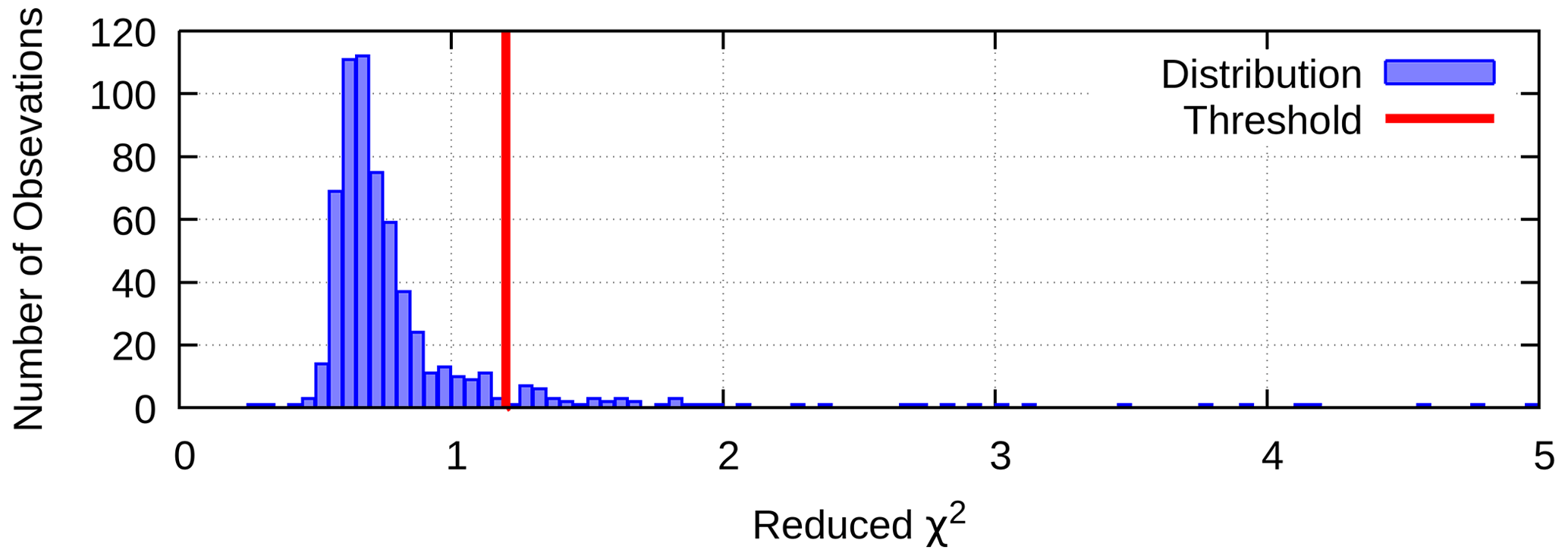
Figure 12Distribution of the reduced χ2 using a bin width of 0.05. The vertical red line at 1.2 indicates the threshold corresponding to an evident minimum (close to zero cases) of the distribution.
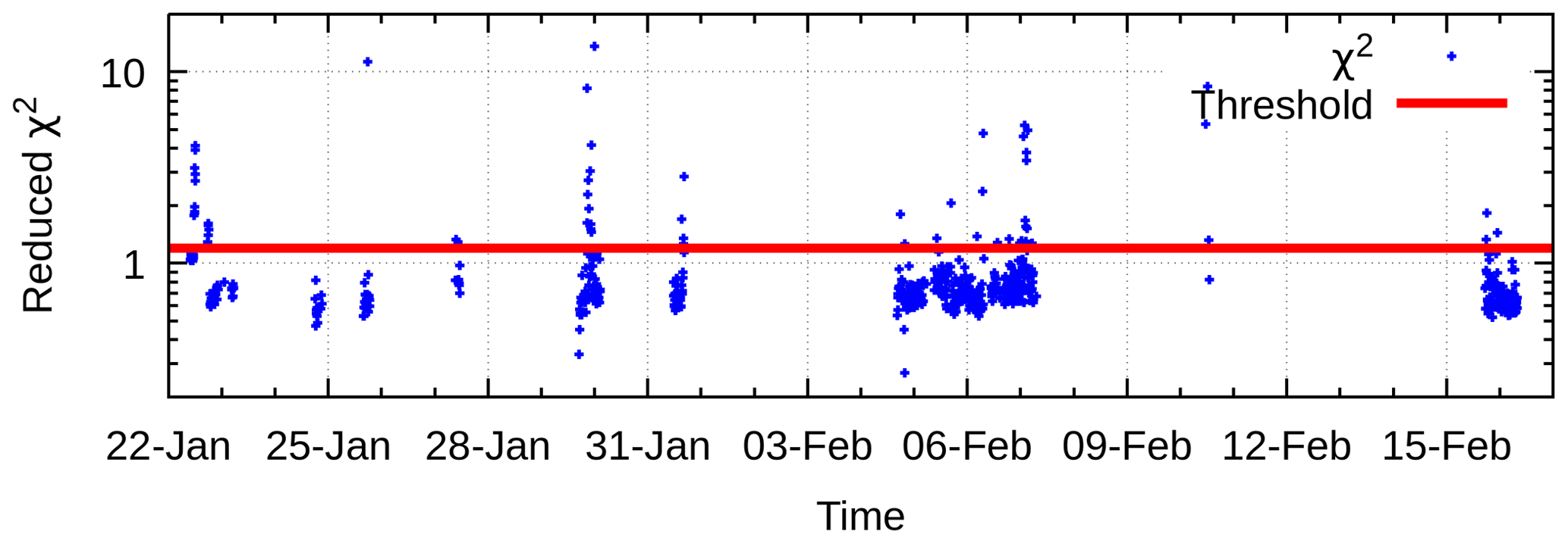
Figure 13Time series of the reduced χ2 obtained from the fitting procedure. Red line indicates the threshold at χ2=1.2 defined in Fig. 12.
Measurements that satisfy the acceptance criterion χ2 were used for a statistical analysis of the residuals. The latter are calculated as the difference between the simulated spectrum at the last iteration of the retrieval and the FIRMOS observation. The mean and standard deviation of residuals provide an a posteriori estimation of the measurements' calibration or forward model error and NESR, respectively.
Figure 14 compares the standard deviation of the residuals (blue line) to the average NESR (red line). The residuals' standard deviation curve correctly reproduces the shape of the average NESR curve of the FIRMOS measurements. However, as observed for the reduced χ2 distribution, the values of the curves indicate a probable overestimation, on average by 25 %, of the NESR of the FIRMOS measurements. The same NESR reduced by 25 % is also shown in green.
Figure 15 shows the comparison between the average of residuals (blue line) and the averaged calibration error (red line). The grey shading is the average NESR divided by the square root of the number of observations (the standard error of the mean). In this case, both the calibration error and the residual NESR are quantitatively consistent with the average of the residuals.
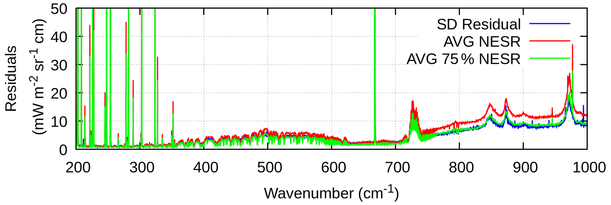
Figure 14Comparison between the standard deviation of the residuals (blue line), the averaged NESR (red line), and the averaged NESR reduced by 25 % (green line).
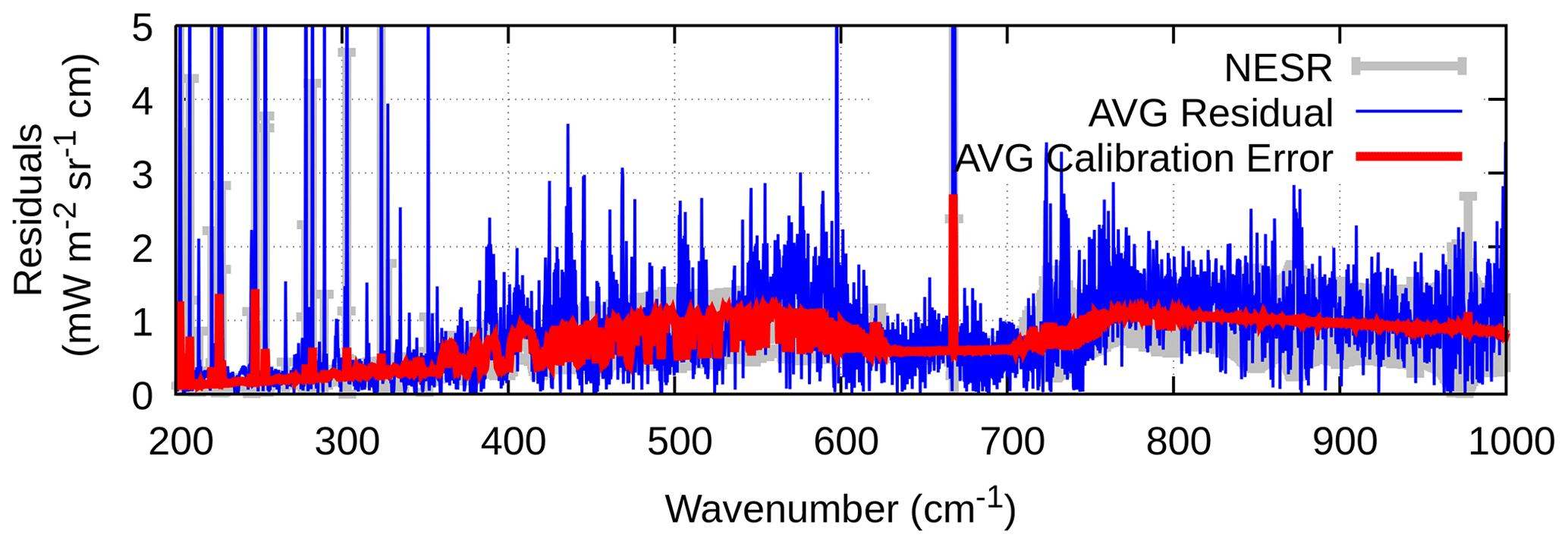
Figure 15Comparison between the average of the residuals (blue line) and the averaged calibration error (red line). The grey shading is the residual NESR after the average.
The vertical distributions of water vapour and temperature were retrieved from FIRMOS observations for six and seven atmospheric levels, respectively (Figs. 18 and 19), from the surface up to 7 km. The time series of the number of the degrees of freedom (DOFs) (Rodgers, 2004) for water vapour (green points) and temperature (red points) profiles are shown in Fig. 16. Within the FIRMOS measurements, we observe strong variability of the information content for water vapour. The temperature also shows some variability in the number of DOFs, although less pronounced than for water vapour. In particular, water vapour shows variations from 2 to 4.5 DOFs and temperature from 1 to 2.5.
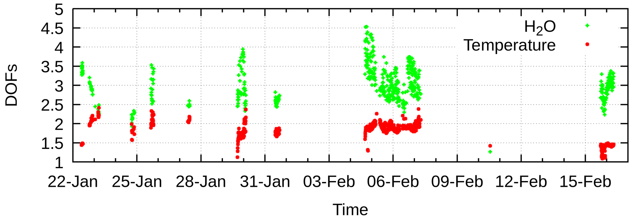
Figure 16Time series of the number of the DOFs of water vapour (green) and temperature (red) profiles obtained from the FIRMOS observations.
The variation in the number of DOFs for the temperature profile is due to the variation of the FIRMOS NESR; indeed, a perfect correlation between the number of DOFs and the average of the inverse of the FIRMOS NESR was found. In contrast, the variation in the number of DOFs in the water vapour profile is associated to the integrated water vapour (IWV) content (Turner and Löhnert, 2014).
As an example, we consider two results respectively with high and low number of DOFs for the water vapour profile. In Fig. 17, water vapour (left) and temperature (right) retrieved profiles are shown, respectively, for the two cases under consideration. The blue curve refers to a high number of DOFs, while the orange curve is for a lower number of the water vapour DOFs. The retrieved IWV content is also indicated in the figure, a higher number of DOFs corresponds to lower IWV and a lower number of DOFs corresponds to higher IWV. In contrast, temperature profiles do not show relevant variations.
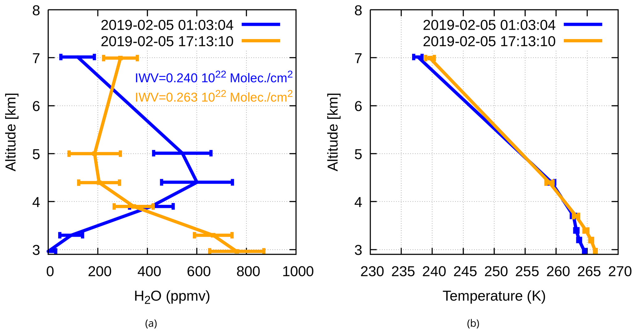
Figure 17(a) Retrieved profiles of the water vapour mixing ratio and of the IWV. (b) Retrieved profiles of the temperature. Error bars correspond to retrieval errors. The profiles were obtained from two FIRMOS measurements with high (blue curves) and low (orange curves) information content. For water vapour, the DOFs are 4.18 and 2.69, respectively, and 2 and 1.78 for temperature, as also shown in Figs. 18 and 19.
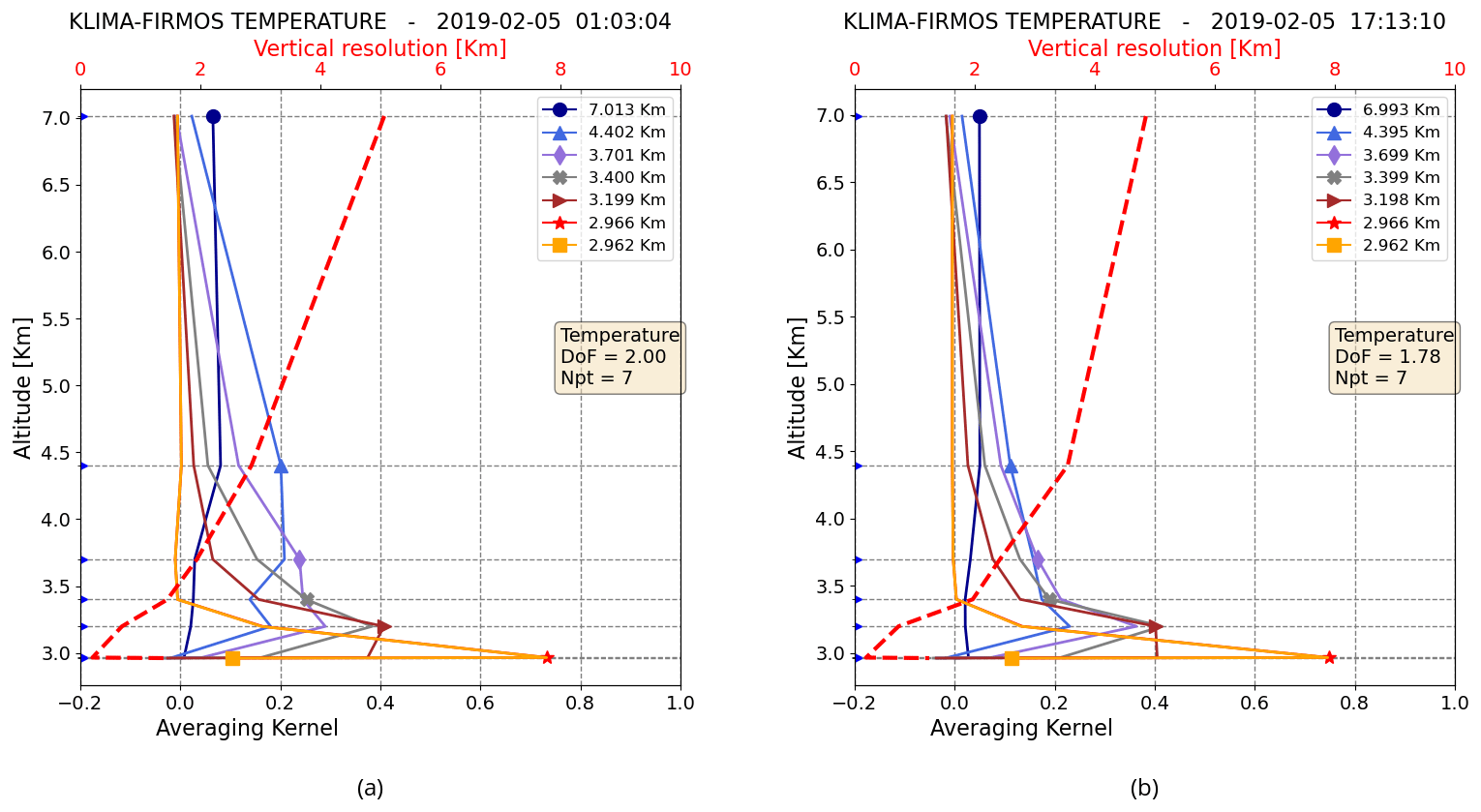
Figures 18 and 19 show the averaging kernel profiles (Rodgers, 2004) for water vapour and temperature, respectively. Retrieved profiles were obtained from two FIRMOS measurements with low (on the left) and high (on the right) IWV content. The vertical resolution profile is also shown (dashed red line). The names of the retrieved species, the total DOFs of the target species, and the number of fitted points are shown in the inset of the figure. High IWV content in the atmosphere reduces the retrieval DOFs, deteriorating the vertical resolution. Instead, the effect of IWV content on temperature retrieval is less significant; both the averaging kernel profiles and the vertical resolution show little variation.
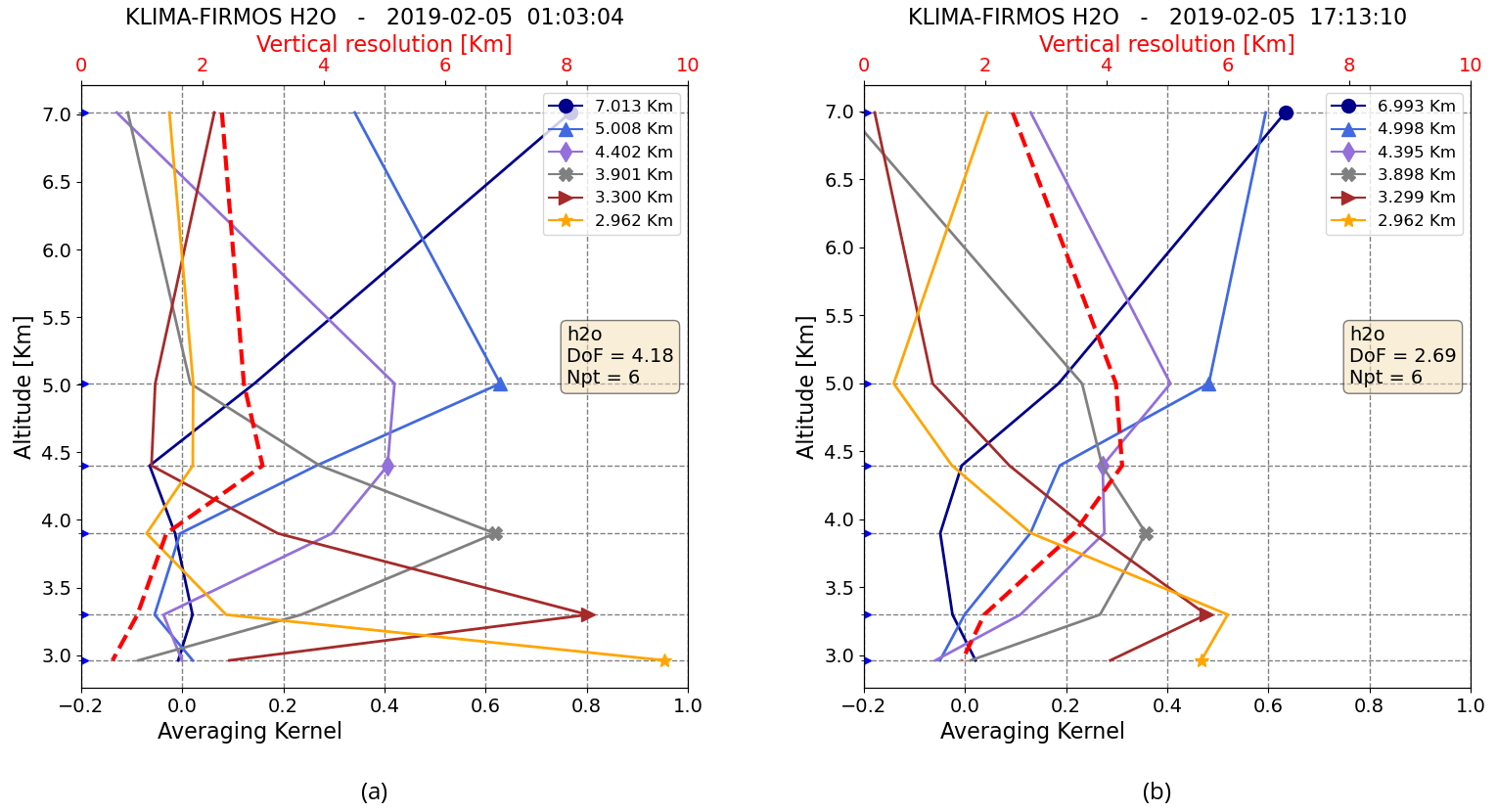
Figure 18Averaging kernel profiles (continuous curves) related to retrieved water vapour profiles as obtained from two FIRMOS measurements with high (a) and low (b) information content. The vertical resolution profile is also reported (dashed red line) (inset). Total DOFs and number of fitted points.
The acquisition of spectra during the campaign experienced some discontinuities, however, during two intervals of the 2019 campaign, between 18:00 CET on 22 January and 06:00 CET on 23 January, and successively between 00:00 CET on 5 February and 06:00 CET on 7 February, FIRMOS observations were sufficiently frequent to create a time series. In order to gain sufficient density, the L2 retrieval results from clear-sky scenes were processed together with the cloudy observations analysed in Di Natale et al. (2021) as mixed and cirrus clouds were identified, mainly, during 5 and 6 February 2019. The single profiles were regridded on a 10 min grid, the time series is presented as a colour-coded map in Fig. 20 to give an overview of the water vapour dataset.
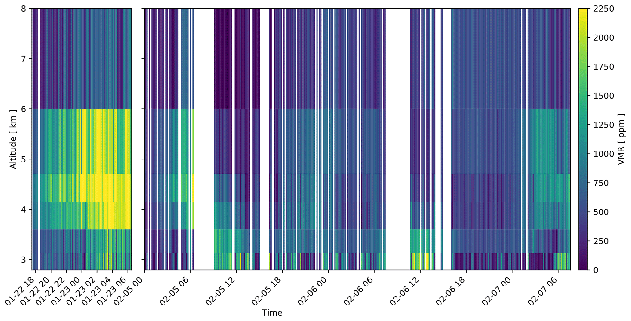
Figure 20Water vapour time series, (left) from 22 January 18:00 to 23 January 06:00 CET, and (right) from 5 February 00:00 to 7 February 06:00 CET in 2019: profiles retrieved from FIRMOS measurements, the single profiles were regridded on a 10 min regular grid.
4.2 Comparisons
The water vapour and temperature profiles retrieved from FIRMOS spectra were compared with those provided by the radiosoundings, those retrieved from the Raman lidar (water vapour only).
4.2.1 Comparison with radiosonde measurements
Five dedicated balloon launches were carried out by a team from the Forschungszentrum Jülich at the Institut für Meteorologie und Klimaforschung (IMK-IFU; part of the Karlsruher Institut für Technologie, KIT) in Garmisch–Partenkirchen, 8.6 km north-east of the summit. The balloons were launched at 18:03, 19:03, and 23:00 CET on 5 February and at 18:33 and 23:33 CET the following day.
Air temperature and water vapour mixing ratio from standard Vaisala RS41-SGP radiosondes were compared to the three individual FIRMOS L2 data nearest in time, in order to evaluate the retrieval products quality. Table 4 lists the measurement time of the FIRMOS data used in the comparison and the corresponding balloon launch.
The RS41 temperature measurement has accuracy of 0.3 K and precision of 0.15 K, the humidity sensor accuracy is 10 % and precision is 2 %, and the quality of the radiosonde water vapour measurements were checked with an accompanied high accurate frostpoint hygrometer (CFH; for details see Palchetti et al., 2021).
Table 4Radiosondes launches on 5 February 2019, and corresponding FIRMOS measurements used in the comparison. The central column specifies the time at which the sonde reached the altitude at which FIRMOS was located. All the times are given in CET time.
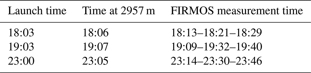
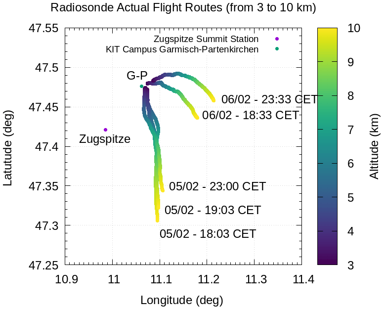
Figure 21Radiosonde actual flight routes limited between 3 and 10 km. The launch times of the balloons in local time are also reported.
Figure 21 shows the radiosonde flight trajectories while their altitude was between 3 and 10 km. The radiosoundings launched on 6 February were under thin cirrus cloud conditions and much farther from Zugspitze, so they were not included in the comparison. The radiosonde profiles have a fine vertical resolution. Therefore, to compare with FIRMOS L2 products, their readings were convolved with the FIRMOS averaging kernels (Rodgers, 2004, AK).
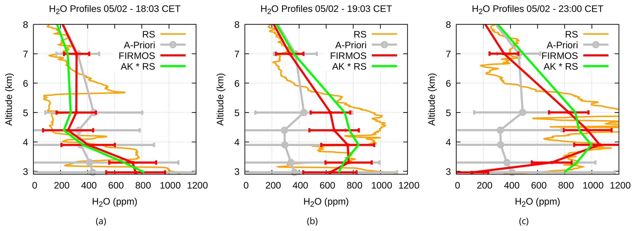
Figure 22Comparison between FIRMOS L2 water vapour product (red curves: mixing ratio) and radiosonde profiles (RS; orange curves: raw data; the green curves are convolved with the FIRMOS AK); a priori profiles are coloured grey. FIRMOS and a priori retrieval errors are also reported. Each plot refers to a different radiosonde acquisition, the local time of the launch is also reported.
Each radio sounding acquired on 5 February was compared to the average of the three profiles of water vapour and temperature retrieved from FIRMOS closest in time (Figs. 22 and 23). Each plot refers to a different radiosonde acquisition, the local time is also reported. The retrieved products are the red curves, and radiosonde profiles before and after the convolution with the FIRMOS AK are the orange and green curves, respectively, a priori profiles are in grey. FIRMOS and a priori retrieval errors are also reported.
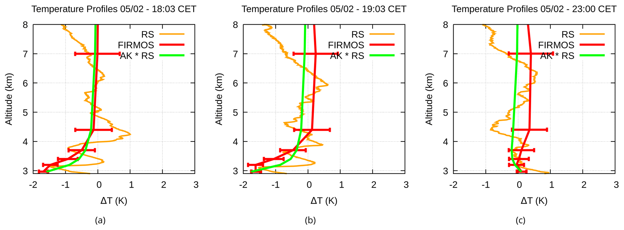
Figure 23Comparison between the FIRMOS L2 temperature product (red curves; the error bars indicate the retrieval error) and radiosonde profiles (orange curves: raw data; the green curves are convolved with the FIRMOS AK). The profiles are shown as a difference with respect to the a priori of the retrieval, for an effective interpretation. Each plot refers to a different radiosonde acquisition, the local time of the radiosonde launch is also reported.
Figure 22 shows how the water vapour profiles retrieved from FIRMOS observations agree with the convolved radiosonde profiles within the retrieval errors. The third radiosonde at the surface is an exception that is probably related to the different boundary conditions experienced by the radiosonde during its trajectory relative to those measured by FIRMOS above the Zugspitze site. Similar to water vapour, the comparison between the temperature obtained from FIRMOS and the convolved radiosonde profiles shows good agreement within the FIRMOS retrieval errors.
4.2.2 Comparisons with Raman lidar measurements at UFS
On 5 and 6 February 2019, a total of four water vapour measurements was carried out with a high-power Raman lidar at UFS. In this period, the stratospheric aerosol lidar was continuously recording backscatter profiles in order to detect the presence of thin cirrus clouds . The lidar systems are described in detail by Klanner et al. (2021; see also Trickl et al., 2020b for more technical details). For water vapour the system features a range from 3 to 20 km a.m.s.l. for a measurement time of 1 h. The data evaluation procedure was recently refined, yielding a better agreement than described by Klanner et al. (2021) with the reference measurements of the campaign. A range extension of up to 25 km could be achieved for measurements with minimal background noise.
The water vapour mixing ratios retrieved from the lidar were calibrated by balloon-borne cryogenic sensors (CFH) of the Forschungszentrum Jülich. The agreement of the lidar measurement with the CFH data was outstanding below 5 km and in the upper troposphere and lower stratosphere in the case of the best time overlap. Between 5 and 8 km, the water vapour mixing ratio exhibited an increasingly spiky humidity structure that was different for lidar and sonde. This is explained by several spatially confined and highly variable dry layers of stratospheric air, unprecedented in spatial inhomogeneity in our lidar sounding over several decades (e.g. Trickl et al., 2014, 2020a, b, and references therein), making the instrument comparison particularly difficult (see Vogelmann et al., 2011, 2015).
The best agreement can be expected for the vertical measurement on the summit and at UFS since the observation volumes almost match. For the lidar, we assume an uncertainty of the order of 5 % on the first 2 d, given the excellent specifications for the CFH sondes. On the third day, the uncertainty can be higher because of the rather distant calibration source.
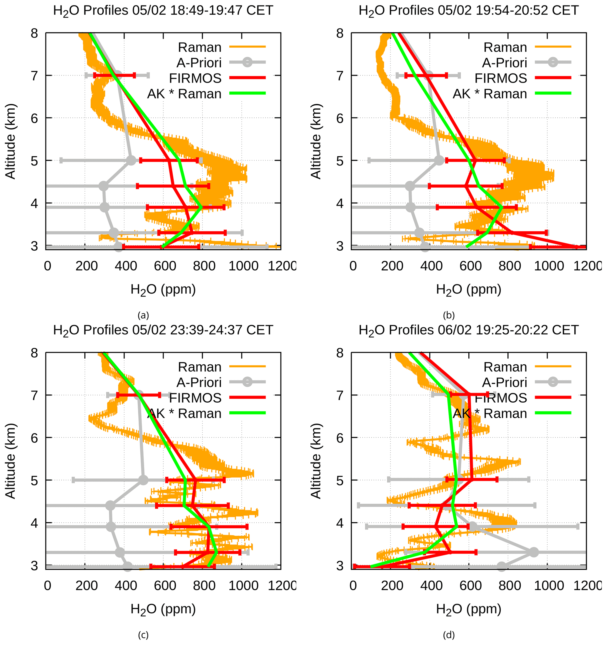
Figure 24Comparison between the FIRMOS L2 water vapour product (red curves) and the Raman profiles (with green curves and without orange curves the convolution with the FIRMOS AK). FIRMOS, a priori, and Raman retrieval errors are also reported. Each plot refers to a different lidar acquisition and the CET time of the acquisition is also reported.
The lidar acquisitions were compared to water vapour profiles retrieved from FIRMOS coincident measurements. The comparison was performed averaging the profiles from five FIRMOS observations for each Raman profile. Given the finer vertical resolution of the Raman profiles, they were convolved with the AK to compare them with FIRMOS L2 products.
Figure 24 shows the comparison between the profiles from FIRMOS L2 water vapour and Raman profiles. Each plot refers to one of the FIRMOS–lidar pairs. The retrieved products are plotted in red, the original Raman profiles in orange, and the green curve is the result of the convolution of the Raman profile with the FIRMOS AK. A priori profiles are shown in grey. FIRMOS, Raman, and a priori retrieval errors are also reported. From Fig. 24 we can conclude that the water vapour profiles retrieved from the FIRMOS observation agreed with the convolved Raman profiles within the retrieval error.
4.2.3 E-AERI radiances comparison
The E-AERI spectrometer at Zugspitze measured in the range 400–1800 cm−1 with a resolution of 0.48215 cm−1 and was positioned 4 m above FIRMOS. To accurately account for the spectral and geometrical differences, the technique described by Tobin et al. (2006) was employed to compare the spectra acquired by the two instruments, calculating the residuals between the observed and the calculated spectra of each instrument, the residuals were then convolved by the other's instrument spectral response function (SRF). Equation (6) defines the radiance differences as follows:
RFIRMOS and RAERI are the mean radiance spectrum for FIRMOS and AERI, respectively; and are the mean simulated radiances; the symbol ∗ denotes the spectral convolution. In RDIFF the residuals are reduced to the lowest common spectral resolution; since the radiance calculations were performed using the same atmospheric state, and forward model physics for both instruments, this results in systematic errors that are common to both sets of calculations, and to first order removes the effects of altitude from the comparison (Tobin et al., 2006).
Figure 25 shows the radiance differences RDIFF, the spectral quantity calculated as in Eq. (6) over 252 coincident spectra, in the range used for the retrieval of IWV (see Sect. 4.2.4). The spectrum in the plot starts at 450, as a suitable number of spectral points are needed to avoid wraparound effects when calculating the convolution. The mean of RDIFF indicates a small positive bias of 0.17 mW m−2 sr−1 cm and a standard deviation of 1.13 mW m−2 sr−1 cm, the total NESR shown in red in the figure is the sum in quadrature of the instruments' individual NESR. The analysis of the radiance differences demonstrates the very good agreement of the two instruments.

4.2.4 E-AERI products comparison
The KIT algorithm for the retrieval of IWV was applied to both the FIRMOS and E-AERI datasets for comparison. IWV is retrieved by minimizing E-AERI (or FIRMOS) versus the line-by-line radiative transfer model (LBLRTM; Clough et al., 2005) spectral residuals in the range from 400 to 600 cm−1 (see Sussmann et al., 2016, for details). The dominant contribution to IWV precision error is the retrieval noise: the higher uncertainty value for FIRMOS precision (0.027 mm) compared to E-AERI (0.020 mm) is related to the higher NESR of FIRMOS compared to E-AERI: ∼2 and ∼0.5 mW m−2 sr−1 cm, respectively.
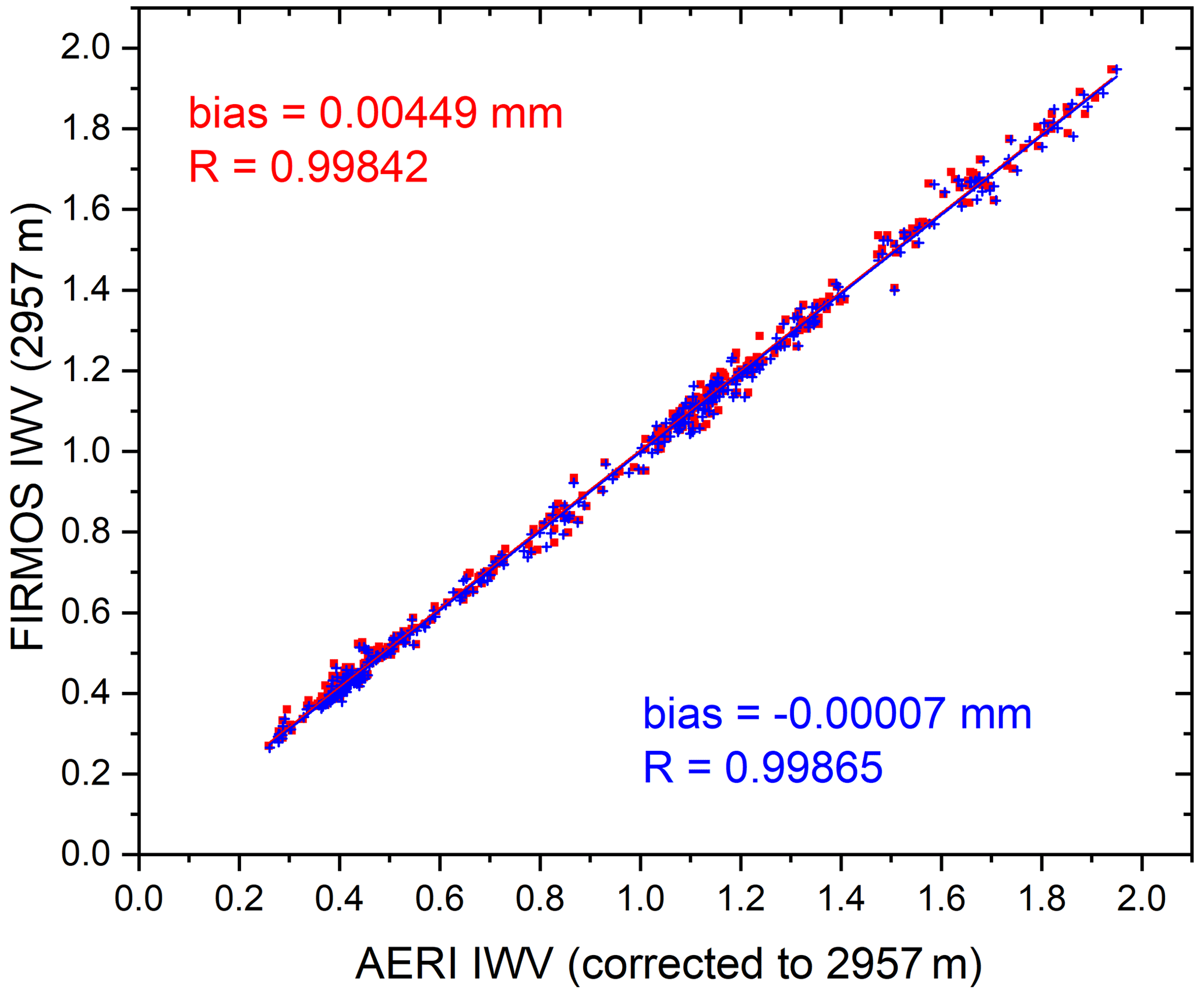
Figure 26IWV values calculated for the two instruments. Red squares: IWV retrieval from AERI spectra and FIRMOS spectra with frequency scale as is. Blue crosses: IWV retrieval from E-AERI and FIRMOS including a joint fit of frequency scale factors (for both instruments independently).
Note that the lower NESR in E-AERI spectra may be explained by E-AERI using a cooled detector (67 K), while FIRMOS uses a room-temperature detector. H2O continuum and line parameters used in the forward calculation and a priori assumptions on the shape of the H2O profile (the NCEP reanalysis as for the FIRMOS L2 data) are factors impacting the accuracy of the IWV retrieval; however, they are common to E-AERI and FIRMOS retrievals and can therefore be disregarded for the IWV intercomparison. Other factors are specific to the instruments and can cause biases between E-AERI and FIRMOS:
-
altitude difference of 4 m between the E-AERI and FIRMOS location;
-
frequency shifts in either or both E-AERI or FIRMOS spectra;
-
calibration errors.
The impact of the altitude difference on IWV (E-AERI: 2961 m a.s.l., FIRMOS: 2957 m a.m.s.l.) was corrected by calculating IWV at the two altitudes from the NCEP profile used as retrieval a priori. The resulting difference used for the altitude correction is 0.002 mm for the mean atmospheric state of the campaign, and therefore the error introduced by this altitude correction should be ≪0.002 mm.
In addition, FTS measurements can show small errors in the frequency scale due to tiny drifts of the calibration laser. As the measured spectrum is fitted to a theoretical spectrum, such frequency errors can propagate to IWV errors in the retrieval process. In fact, direct comparison of coincident FIRMOS and E-AERI spectra (Δt≤4 min) showed evidence of a small discrepancy in frequency scales. Therefore, we implemented a joint fit of a frequency scale factor frequency shift within our IWV retrieval. The resulting mean wavenumber scale factor is 1.0000555 for FIRMOS and 0.9999513 for E-AERI.
The impact from this joint frequency scale retrieval on IWV is shown in Fig. 26. The IWV retrievals with the original spectra are displayed as red squares and there is a bias of δIWV(FIRMOS-AERI) =0.0045 mm. For IWV retrievals with joint frequency scale fit (blue crosses), the bias is practically eliminated to δIWV(FIRMOS-AERI) =0.0002 mm. This bias of 0.0002 mm is negligible compared to the level of measured atmospheric IWV states (from 0.2 to 2 mm H2O); i.e. there are no indications of significant calibration errors in the spectral domain of the H2O rotational band.
In this paper, we describe the FIRMOS Fourier transform spectroradiometer and its performance in detecting the downwelling spectral radiance emitted by the atmosphere. FIRMOS is capable of measuring the atmospheric radiance in the spectral band from 100 to 1000 cm−1 (10–100 µm wavelength) with a spectral resolution of 0.3 cm−1. Its measurement range, in particular, covers the pure rotational band of water vapour in the FIR region, below 667 cm−1 (15 µm), allowing to improve the retrieval performance of water vapour and cloud microphysics. The dominant spectral noise on the calibrated spectrum (NESR) is on average equal to 2 mW m−2 sr−1 cm.
To sound the upper part of the atmosphere, this kind of measurement needs to be performed in extremely dry sites. For this reason, between December 2018 and February 2019, FIRMOS was deployed on the summit of Mount Zugspitze (Germany) at 2957 m a.m.s.l. Out of 838 spectra measured during the campaign, a set of 625 were identified as clear sky and employed to assess the instrument capabilities.
Using the statistical analysis of the difference between the measured spectra and the simulations obtained from the retrieval over the entire clear-sky dataset, we found that the average is comparable with the FIRMOS calibration error indicating the latter is well characterized while the standard deviation suggests a probable overestimation of the NESR.
The radiance measurements were validated with the summit station E-AERI spectroradiometer using the technique described in Tobin et al. (2006) to accurately account for the instruments different spectral characteristics and slightly different viewing geometry. The radiance differences demonstrate the very good agreement of the two instruments. In addition, the FIRMOS measurements were validated by comparing the retrieved IWV values with those obtained from E-AERI. We found a correlation index equal to 0.9986 and a very low bias between the retrieved IWV estimated about −0.00007 mm. This is another confirmation that the FIRMOS and E-AERI spectral measurements are equivalent in their common spectral range.
The retrieved profiles were also found in very good agreement both with the profiles provided by radiosondes launched from Garmisch–Partenkirchen, and by the Raman lidar measuring from UFS at 2675 m a.m.s.l., 700 m to the south-west of the summit station.
FIRMOS was developed to support the FORUM mission, which will be launched by ESA in 2027. FIRMOS was used to validate the measurement method and preliminary instrument design concepts by providing real measurements acquired during a field campaign, the data were used to support the feasibility studies of the mission (ESA, 2019).
In the future, to provide measurements very similar to those that will be delivered by FORUM, it is planned to adapt FIRMOS to stratospheric balloon platforms, this will require to improve instrument subsystems for near-vacuum operations and to cover the full spectral range from 100 to 1600 cm−1 in order to prepare a facility for cal/val activity of the satellite mission.
The full dataset of the 2-month campaign, including infrared spectra (FIRMOS and E-AERI) and all the additional information (lidars, dedicated RS), is available via the ESA campaign dataset website (Palchetti et al., 2020a; https://doi.org/10.5270/ESA-38034ee). ESA requires a free registration to inform users about issues concerning data quality and news on reprocessing. Information about the data formats are reported in README files within each data sub-directory.
LP designed the experiment and was chief scientist for the field campaign. RS was responsible for the local deployment. MB, GB, FD'A, AM, SV ,and LP designed, built, and characterized FIRMOS and carried out the Zugspitze campaign. CB and LP performed the L1 analysis. GDN implemented the clear-sky selection algorithm. SDB, MG, and GDN performed the L2 analysis, FB processed the L2 time series. CR performed the radio soundings and processed their measurements, and SDB and GDN performed the intercomparison analysis. HV and TT performed and processed the lidar measurements, and SDB and GDN performed the intercomparison analysis. MG and SDB performed the spectra intercomparison. RS and MR performed and processed the E-AERI measurements and carried out the IWV intercomparison. CB, GDN, FP, and LP prepared the paper, and CB coordinated the contributions from all co-authors. All authors commented on the paper.
At least one of the (co-)authors is a member of the editorial board of Atmospheric Measurement Techniques. The peer-review process was guided by an independent editor, and the authors also have no other competing interests to declare.
Publisher’s note: Copernicus Publications remains neutral with regard to jurisdictional claims in published maps and institutional affiliations.
This research has been supported by the European Space Agency (FIRMOS Project; contract no. 4000123691/18/NL/LF) and the Agenzia Spaziale Italiana (FORUM scienza project; grant no. 2019-20-HH.0). The dedicated balloon activities were partly funded by Helmholtz–Gemeinschaft (MOSES – Modular Observation Solutions for Earth Systems).
This paper was edited by Frank Hase and reviewed by two anonymous referees.
Bellisario, C., Brindley, H. E., Tett, S. F. B., Rizzi, R., Di Natale, G., Palchetti, L., and Bianchini, G.: Can downwelling far-infrared radiances over Antarctica be estimated from mid-infrared information?, Atmos. Chem. Phys., 19, 7927–7937, https://doi.org/10.5194/acp-19-7927-2019, 2019. a
Bhawar, R., Bianchini, G., Bozzo, A., Cacciani, M., Calvello, M. R., Carlotti, M., Castagnoli, F., Cuomo, V., Di Girolamo, P., Di Iorio, T., Di Liberto, L., di Sarra, A., Esposito, F., Fiocco, G., Fuà, D., Grieco, G., Maestri, T., Masiello, G., Muscari, G., Palchetti, L., Papandrea, E., Pavese, G., Restieri, R., Rizzi, R., Romano, F., Serio, C., Summa, D., Todini, G., and Tosi, E.: Spectrally resolved observations of atmospheric emitted radiance in the H2O rotation band, Geophys. Res. Lett., 35, L04812, https://doi.org/10.1029/2007GL032207, 2008. a
Bianchini, G., Carli, B., Cortesi, U., Del Bianco, S., Gai, M., and Palchetti, L.: Test of far-infrared atmospheric spectroscopy using wide-band balloon-borne measurements of the upwelling radiance, J. Quant. Spectrosc. Ra., 109, 1030–1042, https://doi.org/10.1016/j.jqsrt.2007.11.010, 2008. a, b, c
Bianchini, G., Castagnoli, F., Di Natale, G., and Palchetti, L.: A Fourier transform spectroradiometer for ground-based remote sensing of the atmospheric downwelling long-wave radiance, Atmos. Meas. Tech., 12, 619–635, https://doi.org/10.5194/amt-12-619-2019, 2019. a, b, c, d
Carli, B., Bazzini, G., Castelli, E., Cecchi-Pestellini, C., Del Bianco, S., Dinelli, B. M., Gai, M., Magnani, L., Ridolfi, M., and Santurri, L.: MARC: A code for the retrieval of atmospheric parameters from millimetre-wave limb measurements, J. Quant. Spectrosc. Ra., 105, 476–491, https://doi.org/10.1016/j.jqsrt.2006.11.011, 2007. a
Carlotti, M., Brizzi, G., Papandrea, E., Prevedelli, M., Ridolfi, M., Dinelli, B. M., and Magnani, L.: GMTR: Two-dimensional geo-fit multitarget retrieval model for Michelson Interferometer for Passive Atmospheric Sounding/Environmental Satellite observations, Appl. Optics., 45, 716–727, https://doi.org/10.1364/AO.45.000716, 2006. a
Clough, S. A., Shephard, M. W., Mlawer, E. J., Delamere, J. S., Iacono, M. J., Cady-Pereira, K., Boukabara, S., and Brown, P. D.: Atmospheric radiative transfer modeling: a summary of the AER codes, Short Communication, J. Quant. Spectrosc. Ra., 91, 233–244, 2005. a
Cox, C. V., Harries, J. E., Taylor, J. P., Green, P. D., Baran, A. J., Pickering, J. C., Last, A. E., and Murray, J. E.: Measurement and simulation of mid- and far-infrared spectra in the presence of cirrus, Q. J. Roy. Meteor. Soc., 136, 718–739, https://doi.org/10.1002/qj.596, 2010. a
Del Bianco, S., Carli, B., Gai, M., Laurenza, L. M., and Cortesi, U.: XCO2 retrieved from IASI using KLIMA algorithm, Ann. Geophys., 56, https://doi.org/10.4401/ag-6331, 2013. a
Delamere, J. S., Clough, S. A., Payne, V. H., Mlawer, E. J., Turner, D. D., and Gamache, R. R.: A far-infrared radiative closure study in the Arctic: Application to water vapor, J. Geophys. Res.-Atmos., 115, D17106, https://doi.org/10.1029/2009JD012968, 2010. a
Di Natale, G., Palchetti, L., Bianchini, G., and Del Guasta, M.: Simultaneous retrieval of water vapour, temperature and cirrus clouds properties from measurements of far infrared spectral radiance over the Antarctic Plateau, Atmos. Meas. Tech., 10, 825–837, https://doi.org/10.5194/amt-10-825-2017, 2017. a
Di Natale, G., Barucci, M., Belotti, C., Bianchini, G., D'Amato, F., Del Bianco, S., Gai, M., Montori, A., Sussmann, R., Viciani, S., Vogelmann, H., and Palchetti, L.: Comparison of mid-latitude single- and mixed-phase cloud optical depth from co-located infrared spectrometer and backscatter lidar measurements, Atmos. Meas. Tech., 14, 6749–6758, https://doi.org/10.5194/amt-14-6749-2021, 2021. a, b
ESA: FORUM Report for Mission Selection, Tech. Rep. ESA-EOPSM-FORM-RP-3549, European Space Agency, Noordwijk, the Netherlands, https://esamultimedia.esa.int/docs/EarthObservation/EE9-FORUM-RfMS-ESA-v1.0-FINAL.pdf (last access: 16 March 2023), 2019. a
Harries, J., Carli, B., Rizzi, R., Serio, C., Mlynczak, M., Palchetti, L., Maestri, T., Brindley, H., and Masiello, G.: The Far-infrared Earth, Rev. Geophys., 46, RG4004, https://doi.org/10.1029/2007RG000233, 2008. a
Kanamitsu, M., Ebisuzaki, W., Woollen, J., Yang, S.-K., Hnilo, J. J., Fiorino, M., and Potter, G. L.: NCEP?DOE AMIP-II Reanalysis (R-2), B. Am. Meteorol. Soc., 83, 1631–1644, https://doi.org/10.1175/BAMS-83-11-1631, 2002. a
Klanner, L., Höveler, K., Khordakova, D., Perfahl, M., Rolf, C., Trickl, T., and Vogelmann, H.: A powerful lidar system capable of 1 h measurements of water vapour in the troposphere and the lower stratosphere as well as the temperature in the upper stratosphere and mesosphere, Atmos. Meas. Tech., 14, 531–555, https://doi.org/10.5194/amt-14-531-2021, 2021. a, b, c
Maestri, T., Rizzi, R., Tosi, E., Veglio, P., Palchetti, L., Bianchini, G., Di Girolamo, P., Masiello, G., Serio, C., and Summa, D.: Analysis of cirrus cloud spectral signatures in the far infrared, J. Quant. Spectrosc. Ra., 141, 49–64, https://doi.org/10.1016/j.jqsrt.2014.02.030, 2014. a
Mast, J. C., Mlynczak, M. G., Cageao, R. P., Kratz, D. P., Latvakoski, H., Johnson, D. G., Turner, D. D., and Mlawer, E. J.: Measurements of downwelling far-infrared radiance during the RHUBC-II campaign at Cerro Toco, Chile and comparisons with line-by-line radiative transfer calculations, J. Quant. Spectrosc. Ra., 198, 25–39, https://doi.org/10.1016/j.jqsrt.2017.04.028, 2017. a
Mlawer, E. J., Turner, D. D., Paine, S. N., Palchetti, L., Bianchini, G., Payne, V. H., Cady-Pereira, K. E., Pernak, R. L., Alvarado, M. J., Gombos, D., Delamere, J. S., Mlynczak, M. G., and Mast, J. C.: Analysis of water vapor absorption in the far-infrared and submillimeter regions using surface radiometric measurements from extremely dry locations, J. Geophys. Res.-Atmos., 124, 8134–8160, https://doi.org/10.1029/2018JD029508, 2019. a, b
Mlynczak, M. and Johnson, D.: INFLAME: In-situ net flux within the atmosphere of the Earth, AGU Fall Meeting 2006, San Francisco USA, 11–15 December 2006, EOS Trans. AGU, vol. 87, issue 52, Fall Meeting Supplement, Abstract IN23B-04, 2006. a
Mlynczak, M. G., Cageao, R. P., Mast, J. C., Kratz, D. P., Latvakoski, H., and Johnson, D. G.: Observations of downwelling far-infrared emission at Table Mountain California made by the FIRST instrument, J. Quant. Spectrosc. Ra., 170, 90–105, https://doi.org/10.1016/j.jqsrt.2015.10.017, 2016. a
Palchetti, L., Belotti, C., Bianchini, G., Castagnoli, F., Carli, B., Cortesi, U., Pellegrini, M., Camy-Peyret, C., Jeseck, P., and Té, Y.: Technical note: First spectral measurement of the Earth's upwelling emission using an uncooled wideband Fourier transform spectrometer, Atmos. Chem. Phys., 6, 5025–5030, https://doi.org/10.5194/acp-6-5025-2006, 2006. a
Palchetti, L., Barucci, M., Belotti, C., Bianchini, G., Cluzet, B., D'Amato, F., Del Bianco, S., Di Natale, G., Gai, M., Khordakova, D., Montori, A., Oetjen, H., Rettinger, M., Rolf, C., Schuettemeyer, D., Sussmann, R., Viciani, S., Vogelmann, H., Wienhold, F. G.: FIRMOS – Technical Assistance for a Far-Infrared Radiation Mobile Observation System (EE9 Forum), ESA Earth Observation [data set], https://doi.org/10.5270/ESA-38034ee, 2020a. a
Palchetti, L., Brindley, H., Bantges, R., Buehler, S. A., Camy-Peyret, C., Carli, B., Cortesi, U., Bianco, S. D., Natale, G. D., Dinelli, B. M., Feldman, D., Huang, X. L., C.-Labonnote, L., Libois, Q., Maestri, T., Mlynczak, M. G., Murray, J. E., Oetjen, H., Ridolfi, M., Riese, M., Russell, J., Saunders, R., and Serio, C.: FORUM: Unique Far-Infrared Satellite Observations to Better Understand How Earth Radiates Energy to Space, B. Am. Meteorol. Soc., 101, E2030–E2046, https://doi.org/10.1175/BAMS-D-19-0322.1, 2020b. a, b
Palchetti, L., Barucci, M., Belotti, C., Bianchini, G., Cluzet, B., D'Amato, F., Del Bianco, S., Di Natale, G., Gai, M., Khordakova, D., Montori, A., Oetjen, H., Rettinger, M., Rolf, C., Schuettemeyer, D., Sussmann, R., Viciani, S., Vogelmann, H., and Wienhold, F. G.: Observations of the downwelling far-infrared atmospheric emission at the Zugspitze observatory, Earth Syst. Sci. Data, 13, 4303–4312, https://doi.org/10.5194/essd-13-4303-2021, 2021. a, b, c, d
Ridolfi, M., Del Bianco, S., Di Roma, A., Castelli, E., Belotti, C., Dandini, P., Di Natale, G., Dinelli, B. M., C.-Labonnote, L., and Palchetti, L.: FORUM Earth Explorer 9: Characteristics of Level 2 Products and Synergies with IASI-NG, Remote Sens.-Basel, 12, 1496, https://doi.org/10.3390/rs12091496, 2020. a
Rizzi, R., Arosio, C., Maestri, T., Palchetti, L., Bianchini, G., and Del Guasta, M.: One year of downwelling spectral radiance measurements from 100 to 1400 cm-1 at Dome Concordia: Results in clear conditions, J. Geophys. Res.-Atmos., 121, 10937–10953, https://doi.org/10.1002/2016JD025341, 2016. a
Rizzi, R., Maestri, T., and Arosio, C.: Estimate of Radiosonde Dry Bias From Far-Infrared Measurements on the Antarctic Plateau, J. Geophys. Res.-Atmos., 123, 3205–3211, https://doi.org/10.1002/2017JD027874, 2018. a
Rodgers, C. D.: Inverse methods for atmospheric sounding: theory and practice, Vol. 2, in: Series on atmospheric oceanic and planetary physics, World Scientific, Singapore, reprinted 2004, oCLC: 254137862, ISBN 981-02-2740-X, 2004. a, b, c, d
Sgheri, L., Belotti, C., Ben-Yami, M., Bianchini, G., Carnicero Dominguez, B., Cortesi, U., Cossich, W., Del Bianco, S., Di Natale, G., Guardabrazo, T., Lajas, D., Maestri, T., Magurno, D., Oetjen, H., Raspollini, P., and Sgattoni, C.: The FORUM end-to-end simulator project: architecture and results, Atmos. Meas. Tech., 15, 573–604, https://doi.org/10.5194/amt-15-573-2022, 2022. a
Sussmann, R., Reichert, A., and Rettinger, M.: The Zugspitze radiative closure experiment for quantifying water vapor absorption over the terrestrial and solar infrared – Part 1: Setup, uncertainty analysis, and assessment of far-infrared water vapor continuum, Atmos. Chem. Phys., 16, 11649–11669, https://doi.org/10.5194/acp-16-11649-2016, 2016. a, b
Tobin, D. C., Revercomb, H. E., Knuteson, R. O., Best, F. A., Smith, W. L., Ciganovich, N. N., Dedecker, R. G., Dutcher, S., Ellington, S. D., Garcia, R. K., Howell, H. B., LaPorte, D. D., Mango, S. A., Pagano, T. S., Taylor, J. K., van Delst, P., Vinson, K. H., and Werner, M. W.: Radiometric and spectral validation of Atmospheric Infrared Sounder observations with the aircraft-based Scanning High-Resolution Interferometer Sounder, J. Geophys. Res.-Atmos., 111, D09S02, https://doi.org/10.1029/2005JD006094, 2006. a, b, c
Trickl, T., Vogelmann, H., Giehl, H., Scheel, H.-E., Sprenger, M., and Stohl, A.: How stratospheric are deep stratospheric intrusions?, Atmos. Chem. Phys., 14, 9941–9961, https://doi.org/10.5194/acp-14-9941-2014, 2014. a
Trickl, T., Giehl, H., Neidl, F., Perfahl, M., and Vogelmann, H.: Three decades of tropospheric ozone lidar development at Garmisch-Partenkirchen, Germany, Atmos. Meas. Tech., 13, 6357–6390, https://doi.org/10.5194/amt-13-6357-2020, 2020a. a
Trickl, T., Vogelmann, H., Ries, L., and Sprenger, M.: Very high stratospheric influence observed in the free troposphere over the northern Alps – just a local phenomenon?, Atmos. Chem. Phys., 20, 243–266, https://doi.org/10.5194/acp-20-243-2020, 2020b. a, b
Turner, D. D. and Löhnert, U.: Information Content and Uncertainties in Thermodynamic Profiles and Liquid Cloud Properties Retrieved from the Ground-Based Atmospheric Emitted Radiance Interferometer (AERI), J. Appl. Meteorol. Clim., 53, 752–771, https://doi.org/10.1175/JAMC-D-13-0126.1, 2014. a
Turner, D. D. and Mlawer, E. J.: The Radiative Heating in Underexplored Bands Campaigns, B. Am. Meteorol. Soc., 91, 911–924, https://doi.org/10.1175/2010BAMS2904.1, 2010. a
Turner, D. D., Mlawer, E. J., Bianchini, G., Cadeddu, M. P., Crewell, S., Delamere, J. S., Knuteson, R. O., Maschwitz, G., Mlynczak, M., Paine, S., Palchetti, L., and Tobin, D. C.: Ground-based high spectral resolution observations of the entire terrestrial spectrum under extremely dry conditions, Geophys. Res. Lett., 39, L10801, https://doi.org/10.1029/2012GL051542, 2012. a
Vogelmann, H., Sussmann, R., Trickl, T., and Borsdorff, T.: Intercomparison of atmospheric water vapor soundings from the differential absorption lidar (DIAL) and the solar FTIR system on Mt. Zugspitze, Atmos. Meas. Tech., 4, 835–841, https://doi.org/10.5194/amt-4-835-2011, 2011. a
Vogelmann, H., Sussmann, R., Trickl, T., and Reichert, A.: Spatiotemporal variability of water vapor investigated using lidar and FTIR vertical soundings above the Zugspitze, Atmos. Chem. Phys., 15, 3135–3148, https://doi.org/10.5194/acp-15-3135-2015, 2015. a