the Creative Commons Attribution 4.0 License.
the Creative Commons Attribution 4.0 License.
 | 06 Jun 2023
The classification of atmospheric hydrometeors and aerosols from the EarthCARE radar and lidar: the A-TC, C-TC and AC-TC products
Abdanour Irbah
Julien Delanoë
Gerd-Jan van Zadelhoff
David P. Donovan
Pavlos Kollias
Bernat Puigdomènech Treserras
Shannon Mason
Robin J. Hogan
Aleksandra Tatarevic
The EarthCARE mission aims to probe the Earth's atmosphere by measuring cloud and aerosol profiles using its active instruments, the Cloud Profiling Radar (CPR) and ATmospheric LIDar (ATLID). The correct identification of hydrometeors and aerosols from atmospheric profiles is an important step in retrieving the properties of clouds, aerosols and precipitation. Ambiguities in the nature of atmospheric targets can be removed using the synergy of collocated radar and lidar measurements, which is based on the complementary spectral response of radar and lidar relative to atmospheric targets present in the profiles. The instruments are sensitive to different parts of the particle size distribution and provide independent but overlapping information in optical and microwave wavelengths. ATLID is sensitive to aerosols and small cloud particles, and CPR is sensitive to large ice particles, snowflakes and raindrops. It is therefore possible to better classify atmospheric targets when collocated radar and lidar measurements exist compared to using a single instrument. The cloud phase, precipitation and aerosol type within the column sampled by the two instruments can then be identified. ATLID-CPR target classification (AC-TC) is the product created for this purpose by combining the ATLID target classification (A-TC) and CPR target classification (C-TC). AC-TC is crucial for the subsequent synergistic retrieval of cloud, aerosol and precipitation properties. AC-TC builds upon previous target classifications using CloudSat and CALIPSO synergy while providing richer target classification using the enhanced capabilities of EarthCARE's instruments, specifically CPR's Doppler velocity measurements to distinguish snow and rimed snow from ice clouds and ATLID's lidar ratio measurements to objectively discriminate between different aerosol species and optically thin ice clouds. In this paper, we first describe how the single-instrument A-TC and C-TC products are derived from ATLID and CPR measurements. Then the AC-TC product, which combines the A-TC and C-TC classifications using a synergistic decision matrix, is presented. Simulated EarthCARE observations based on combined cloud-resolving and aerosol model data are used to test the processors generating the target classifications. Finally, the target classifications are evaluated by quantifying the fractions of ice and snow, liquid clouds, rain, and aerosols in the atmosphere that can be successfully identified by each instrument and their synergy. We show that radar–lidar synergy helps better detect ice and snow, with ATLID detecting radiatively important optically thin cirrus and cloud tops, while CPR penetrates most deep and highly concentrated ice clouds. The detection of rain and drizzle is entirely due to C-TC, while that of liquid clouds and aerosols is due to A-TC. The evaluation also shows that simple assumptions can be made to compensate for when the instruments are obscured by extinction (ATLID) or surface clutter and multiple scattering (CPR); this allows for the recovery of the majority of liquid cloud not detected by the active instruments.
- Article
(11483 KB) - Full-text XML
- BibTeX
- EndNote


Clouds and aerosols play an essential role in the Earth's radiation balance and condition the temperature of the atmosphere on very variable timescales. A large-scale knowledge of their life cycle and spatial extent is therefore important to understand the climate of the Earth and to predict weather conditions. The EarthCARE mission was designed to provide some answers to this complex subject, particularly for a better understanding of the interactions between clouds, aerosols and radiation, which is necessary for the improvement of numerical weather prediction models (Illingworth et al., 2015).
EarthCARE is a joint ESA (European Space Agency)/JAXA (Japan Aerospace Exploration Agency) mission scheduled for launch in 2024 (Wehr et al., 2023). The satellite will be in a sun-synchronous orbit with a 25 d repetition cycle and at low altitude (around 408 km) in order to maximise the sensitivity of its instruments (do Carmo et al., 2021). Its two active instruments are ATLID (ATmospheric LIDar), a high-spectral-resolution lidar (HSRL) operating at 355 nm, and CPR (Cloud Profiling Radar), a Doppler radar operating at 94 GHz. A full description of the payload is given in Wehr et al. (2023). EarthCARE's radar and lidar invite comparisons with the following active instruments in the A-Train constellation (Stephens et al., 2018): CloudSat's CPR (Stephens et al., 2008) and CALIOP (Cloud–Aerosol Lidar with Orthogonal Polarization) aboard CALIPSO (Winker et al., 2010). The larger antenna and lower orbit of EarthCARE's CPR offers around 7 dBZ higher sensitivity than CloudSat, and its Doppler capability will facilitate richer observations of cloud and precipitation by measuring the vertical motion of hydrometeors; more details on the specification of the two radars can be found in Burns et al. (2016) and Illingworth et al. (2015). ATLID's 355 nm wavelength means the backscattering properties of clouds and aerosols and the atmosphere will be different from those of CALIOP at 532 nm, while its smaller field of view and narrower filter will reduce daytime background noise. With its HSRL capability for distinguishing Rayleigh (molecular) from Mie (particulate) backscatter, ATLID will be better able to discriminate types of aerosol and optically thin ice clouds (Illingworth et al., 2015). The main advantage of joint radar–lidar observations is that the two instruments provide complementary spectral responses to the targets in the column that they sample; that is, each instrument is sensitive to different parts of the particle size distribution. Independent but overlapping information from the microwave and optical spectral domains is obtained by joint observations from radar and lidar. The lidar is sensitive to the smallest particles (aerosols, ice particles and cloud droplets), and the radar is sensitive to larger ones such as snowflakes and raindrops. Thus, some ambiguities in the detection made by one instrument will be compensated for by the sensitivities of the other. An essential first step before inferring the properties of cloud, precipitation and aerosols in a retrieval algorithm is to reliably locate and identify the types of targets detected throughout the atmospheric profile. In some respects, the two instruments detect complementary parts of the atmosphere – aerosol typing will rely only on lidar measurements, and precipitation will rely solely on radar observations – but the detection and identification of ice, liquid and mixed-phase clouds benefits enormously from the synergy of radar and lidar (Ceccaldi et al., 2013). In designing target classification processors for EarthCARE's active instruments, we therefore benefit from the past experiences of using radar–lidar measurements from ground-based (CloudNet; Illingworth et al., 2007) and satellite (DARDAR-MASK; Ceccaldi et al., 2013; Delanoë and Hogan, 2010) observations. The EarthCARE synergistic product is constructed differently than DARDAR-MASK, although both are basically based on the same approach. Indeed, the radar–lidar measurements are combined at each altitude grid point to create a synergistic target classification product in a single step thanks to the already existing and validated EarthCARE products, A-TC and C-TC. The EarthCARE production model (Eisinger et al., 2023) allows for target classifications from ATLID (A-TC) and CPR (C-TC) to be encapsulated in distinct L2a products, which are used for single-instrument retrieval products such as the CPR cloud and precipitation retrieval (C-CLD; Kollias et al., 2022) and ATLID ice cloud retrieval (A-ICE; Donovan et al., 2023a). A-TC and C-TC encode the types of targets relevant to each instrument, namely liquid clouds, ice clouds and aerosols by ATLID and liquid clouds, drizzle and rain, ice clouds, and snow by CPR. The single-instrument target classifications A-TC and C-TC are then merged, without the need to reanalyse their measurements, into the synergistic target classification product (AC-TC), which should, in all cases, be consistent with – or superior to – the single-instrument products. AC-TC is a necessary input to EarthCARE's synergistic retrieval of clouds, aerosols and precipitation (ACM-CAP; Mason et al., 2022). While EarthCARE's synergistic target classification will make use of the enhanced capabilities of ATLID and CPR to make distinctions in aerosol species and precipitation type that were not possible for CloudSat-CALIPSO, it is expected that AC-TC will facilitate continuity with DARDAR-MASK. Like DARDAR-MASK, the AC-TC product will also be used to derive important statistics of the spatial and temporal distributions and structures of aerosols, clouds and precipitation, as well as their properties and thermodynamic phase (e.g. Huang et al., 2012; Mason et al., 2014; Mioche et al., 2015, 2017; Mülmenstädt et al., 2015; Vérèmes et al., 2019; Listowski et al., 2019, 2020).
In this paper, we first describe how single-instrument target classifications are derived from ATLID (A-TC; Sect. 2) and CPR (C-TC; Sect. 3). The decision matrix used to produce the synergistic target classification AC-TC is then detailed in Sect. 4. The tests and results obtained with the processors developed for the calculation of A-TC, C-TC and AC-TC will then be presented (Sect. 5), making use of simulated data from one of the EarthCARE test scenes derived from high-resolution model data as described in Qu et al. (2022) and Donovan et al. (2023a). In Sect. 6, the performance of the single-instrument and synergistic target classifications will be evaluated by quantifying the extent to which they accurately resolve the amounts of aerosols, clouds and precipitation present in the numerical weather model used to create the simulated test scenes. Finally, we summarise the performance of the target classification products and discuss the contributions of AC-TC to EarthCARE science (Sect. 7).
The range-resolved ATLID observations provide information about the vertical and horizontal structure of aerosol and clouds and their respective sub-typing. Identification of these (sub-)types is based on the use of the ATLID depolarisation signals, temperature, altitude, the extinction and backscatter profiles, and the corresponding lidar ratio. For this retrieval, the ATLID target classification (A-TC) module has been created. The A-TC procedures are applied to layers which are assumed to be homogeneous. Both the layering determination and the subsequent classification procedures are called from either the large-scale aerosol (and thin cloud) extinction and backscatter (A-AER) algorithm or the optimal-estimation Extinction and Backscatter retrieval algorithm (A-EBD). The A-AER and A-EBD procedures are components of the ATLID profile processor (A-PRO) described in Donovan et al. (2023b). The A-PRO processor also generates the A-TC product.
The A-TC classification main inputs are per-layer estimates of the particulate (Mie) extinction (αMie) and backscatter (βMie), lidar ratio (S), the linear depolarisation ratio (δ), and the attenuated particulate backscatter (ATBM). Error estimates for all these quantities are also required. In addition to the lidar-derived quantities, meteorological data (e.g. temperature and tropopause height) are supplied by the ECMWF (European Centre for Medium-Range Weather Forecasts) in the form of the X-MET EarthCARE auxiliary product (Eisinger et al., 2023). The main algorithm follows a decision tree structure in which various conditional thresholds are applied. Here, a brief treatment is presented; more details can be found in Donovan et al. (2023b).
The creation of the target classification involves four main sub-procedures. The four main sub-procedures are as follows, with the output of each procedure serving as input to the subsequent ones:
- 1.
layering determination
- 2.
simple (fall-back) classification
- 3.
detailed classification
- 4.
hybrid-mode classification smoothing.
Each of these steps are described in turn in the following sub-sections.
2.1 Layer determination
The layer determination procedures that are implemented within A-PRO are necessary, in part, due to the need for averaging in order to increase the signal-to-noise ratio of the lidar-derived inputs. The procedures for determining layers are implemented as a part of the A-AER algorithm described in detail within Donovan et al. (2023b); here, a brief overview of the layer determination procedures is given. The layering determination is a two-step procedure, a coarse-layering determination and a subsequent layer-splitting procedure.
2.1.1 Coarse layering
The coarse layering is determined using the input ATLID-featuremask (A-FM). The A-FM product provides a probability mask for the existence of atmospheric features within the lidar profile product (van Zadelhoff et al., 2023b) at the native ATLID resolution. The A-FM is re-gridded to the joint standard grid (JSG; Eisinger et al., 2023) by selecting the maximum featuremask value present within each JSG pixel, except in the case of surface detections. Each data column is then treated in turn, and layer boundaries are assigned whenever
- 1.
a transition between clear-sky featuremask values (as determined by the threshold, e.g. 5) and significant featuremask values exists between two adjacent featuremask values,
- 2.
the absolute difference between two adjacent featuremask values exceeds a defined threshold,
- 3.
a transition between featuremask values exceeding the clear-sky threshold and attenuated or surface pixels exists,
- 4.
the lidar-scattering ratio () calculated by A-AER crosses a set threshold (e.g. 10).
Steps (1) and (2) produce layer boundaries where transitions between significant features and clear-sky exist or where transitions between weak and strong features exist. Step (3) assigns layer boundaries when the point of attenuation in the lidar signal is reached. Step (4) assigns layer boundaries when the absolute value of the change in R exceeds a given threshold, e.g. near the top and bottom of layers (e.g. water clouds) but not around layer peaks. As an option, layer boundaries can be assigned when the temperature crosses 0 ∘C and/or when the temperature crosses −40 ∘C (homogeneous-freezing threshold).
2.1.2 Layer splitting
After the coarse-layer structure is determined, each layer by itself is examined to see if the layer should be further subdivided. The basic idea is to test to see if it is valid to represent the layer as a homogeneous entity or if it is better to split the layer into a number of homogeneous sub-layers. The procedure relies on examining the behaviour of a reduced chi-squared goodness-of-fit variable applied to the scattering ratio, lidar ratio and the depolarisation ratio which is calculated for all possible sub-layering for up to four distinct sub-layers (depending on the extend of the coarse layer). For example, for the case of two sub-layers, we have the following:
where N is the number of sub-layers being considered (two in this case), and nl1 is the depth of the first sub-layer. In general,
where Q is used to represent the quantity in question, i.e. the A-AER-calculated scattering ratio (), the lidar ratio (extinction-to-backscatter ratio; ) and the linear depolarisation ratio (). The σs represent the appropriate uncertainty estimate, nc is the coarse-layer depth, and represents the mean of the quantity in question (R, S or δ) evaluated for the sub-layering structure in question. Only those quantities which have been successfully retrieved are used; e.g. if, for a layer, the S ratio is not valid, it is not used.
For each trial number of sub-layers, the lowest value of, e.g. in the case of two layers, or, e.g. for two sub-layers, is selected and forms the sequence . The sequence of values is then examined to decide on the number of sub-layers to assign to the coarse layer. The number of sub-layers is chosen if either
-
an increase in N results in a large drop in (i.e a relative decrease set by a defined threshold e.g. a factor of 10) compared to the proceeding value of N, or
-
a subsequent increase in N does not result in a relative decrease in that is better than some defined threshold (e.g. 10 %).
Once the optimal number of sub-layers is decided upon, the sub-layering structure corresponding to the selected value of is imposed upon the coarse layer, and the layering structure for the column in question is updated.
2.2 Simple classification
The simple-classification procedure serves as input to the more detailed-classification procedure and as a fall-back when the more detailed-classification procedure can not be (fully) applied due to e.g. not all input variables required for the detailed procedure being valid. The procedure can also alter the layering structure to ensure that layers do not span the tropopause.
The main steps of the simple-classification procedure are depicted in Fig. 1. First, a crude aerosol–cloud separation is performed using a threshold test based on the scattering ratio (R). The threshold itself (Rcld(z)) is a function of height and decreases with height as a function of atmospheric density, i.e.
where ρ is the atmospheric density. A threshold of Rcld=5 was found to work well for the test scenes. It should be mentioned that this value (along with any other thresholds mentioned in this work) is provisional and will be refined using actual observations in the commissioning phase of the mission after launch. For cloudy layers, the layer mean wet-bulb temperature, i.e. (where n is the extent of the layer), is compared to both the melting temperature and the homogeneous-freezing temperature. A second scattering ratio test, this one aimed at identify large scattering ratios associated with water clouds, is also applied (Rwater=10, which is density dependent in a manner similar to Rcld). Finally, for layers not yet assigned as being liquid or ice, the integrated-depolarisation-to-integrated-backscatter ratio is examined. Values of this ratio above 1×10⁴ are interpreted as being indicative of ice clouds.
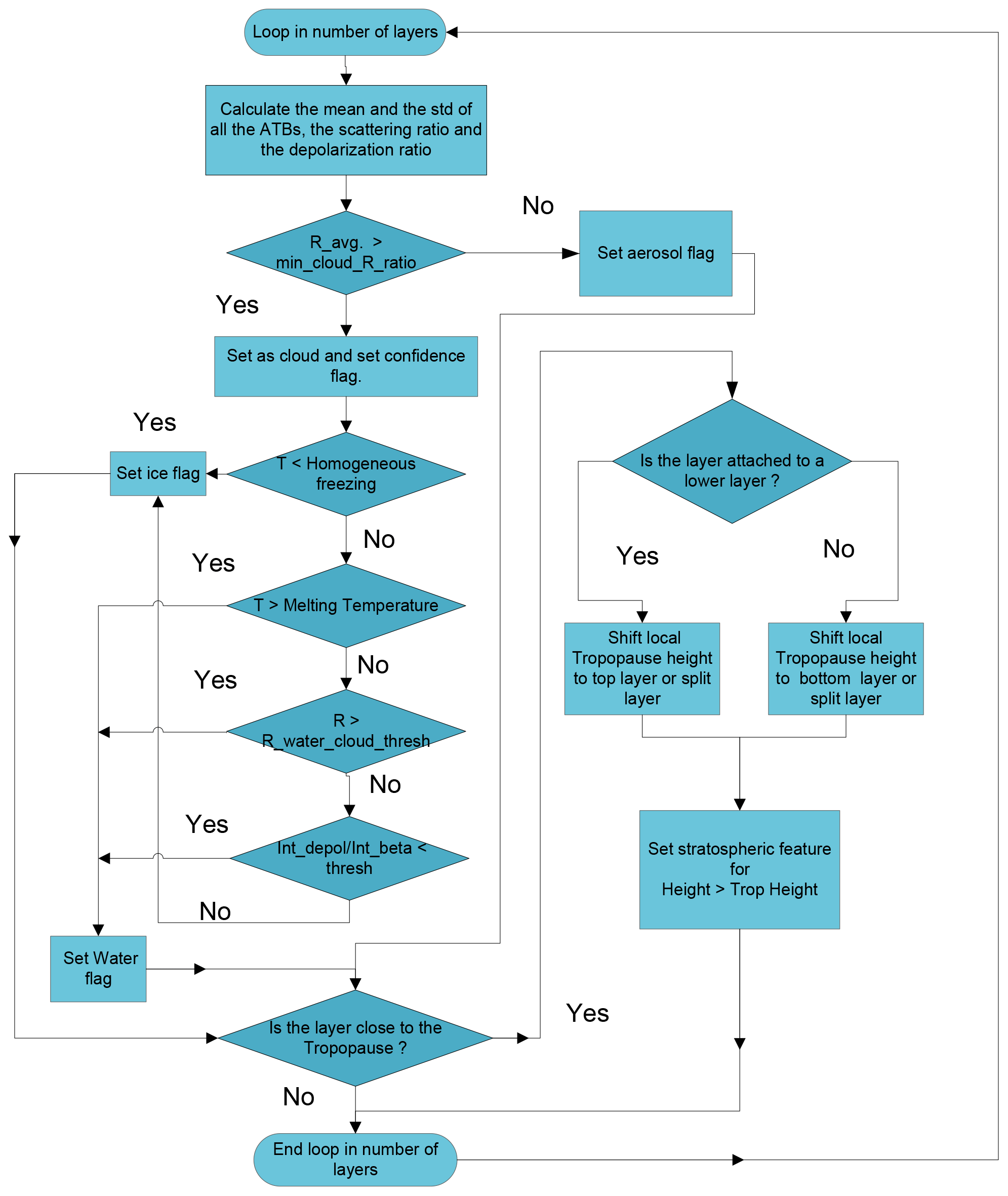
After the layer “simple class” has been assigned, layers spanning the tropopause height are further scrutinised. Layers which can be split while leaving no layer smaller than three pixels in vertical extent are split at the tropopause height. If this is not the case, then the tropopause level is itself adjusted. The logic for this procedure is linked to the fact that the tropopause height estimate may itself be uncertain.
2.3 Detailed classification
The main steps of the detailed-classification procedure are depicted in Fig. 2.
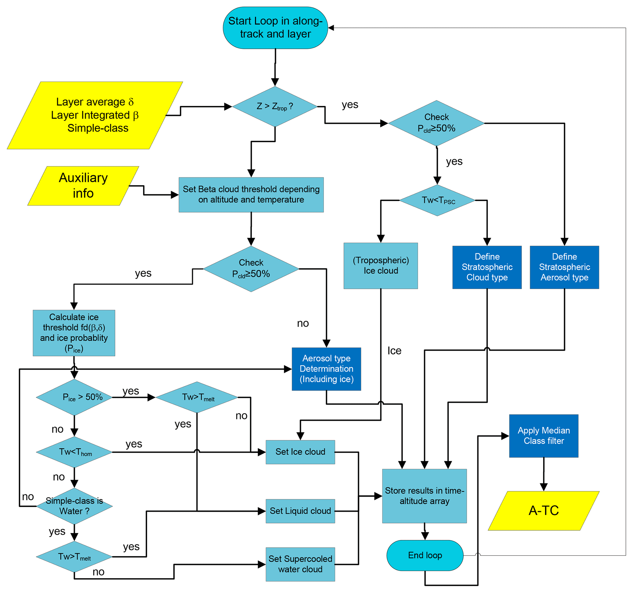
2.3.1 Tropospheric cloud and aerosol discrimination
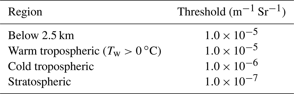
For layers whose top is at or below the tropopause level, the first step in the A-TC classification procedure is to perform the cloud–aerosol separation based on a threshold applied to the layer mean Mie backscatter. This threshold can be specified as a look-up table based on altitude and temperature. By default, four temperature–altitude regions are defined and presented in Table 1. The reader is reminded that it is expected that this scheme will be updated on the basis of observations during the commissioning phase. Layers that exceed the threshold are classified as being clouds. Layers that do not meet this threshold are provisionally treated as being aerosol or thin ice clouds in case the mean layer temperature is below freezing. Layers classified as being water clouds in the input simple classification will also be set to water clouds on the basis of this previous assignment.
Table 1ATLID default cloud backscatter thresholds (detailed procedure).
2.3.2 Cloud phase determination
Layers identified as cloud then undergo a cloud phase determination step. Here, the layer-integrated linear depolarisation ratio and attenuated backscatters are used in a manner similar to that used in CALIPSO data processing. Hu et al. (2009) showed that this combination of parameters can effectively discriminate ice from liquid and horizontally oriented ice crystals. The liquid water relationship was calculated using Monte-Carlo lidar radiative transfer simulation results (Hu et al., 2007) for a range of extinctions and particle sizes. For ATLID lidar, Monte Carlo simulations have shown that the relationship between layer-integrated attenuated backscatter and layer depolarisation is expected to be similar to those measured by CALIPSO (Donovan et al., 2015). Liquid layers whose layer mean temperature is below freezing are classified as supercooled water layers.
2.3.3 Aerosol type determination (including ice)
For areas classified as containing aerosols (or thin ice) only, A-TC contains procedures for assigning probabilistic aerosol types. For the aerosol classification, a suitable set of basic aerosol types must be defined. This basic set must be complete enough to reasonably encompass the range of types encountered in nature but should not be more extensive than justified by the measurements so that the basic number of types is tractable. The classification should allow the separation of natural and anthropogenic aerosols. The types need to be described consistently in terms of microphysical properties (size, shape and refractive index), which are used to represent them in scattering models, and in terms of optical and radiative properties, which are observed with the EarthCARE instruments and are used for the classification (lidar ratio, linear depolarisation ratio and Ångström exponent).
To assist all the EarthCARE processors, the Hybrid End-To-End Aerosol Classification (HETEAC) model for the EarthCARE mission (Wandinger et al., 2023) has been defined based on ground and aircraft observations. The HETEAC model aims to ensure that the different aerosol products from the multi-instrument platform are consistent for all EarthCARE processors, including the definition of the broadband optical properties needed for the EarthCARE radiative closure.
Based on the HETEAC framework, 2D-oriented Gaussian distributions in the linear depolarisation ratio δ and lidar ratio S are defined for each aerosol class (see Fig. 3). Each class is defined by a central δ, S position, effective Gaussian widths in each dimension and the correlation between δ and S.
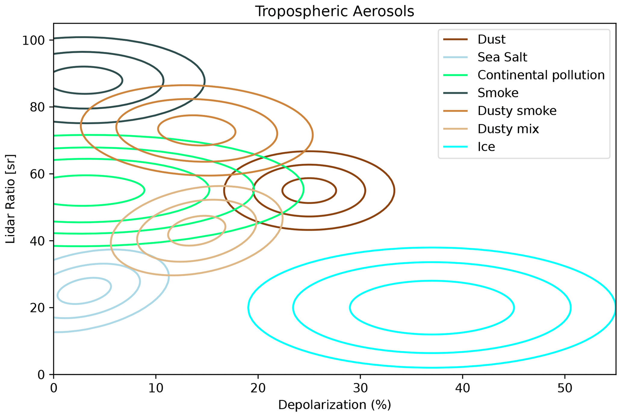
Figure 3Probability density distributions for the six aerosol types and ice crystals currently being used within A-TC.
All the classification parameters are defined in a configuration file to make the validation and updating of the algorithm to new parameterisations straightforward. The central δm, S positions and associated 1σ values for each of the particle types will need to be validated in a future effort. For each observed combination of the observed layer lidar ratio and depolarisation, the probability that the layer belongs to each defined class is calculated based on Gaussian statistics. The type probabilities are the main results from the procedure; however, the most probable type is provided in the output. In cases where a single type is not dominant or where all classes have a low associated probability, then an unknown classification may result.
2.3.4 Additional ice aerosol separation
Ice crystals are also treated as an aerosol type, since they span part of the δ–S parameter space not occupied by aerosols (see Fig. 3). This is used to further refine the separation between thin ice clouds from aerosol fields. This is required, since the backscatter-threshold-based cloud aerosol separation step applied earlier tends to produce halos of aerosol around upper-level ice clouds.
For layers identified as thin ice by the δ–S-based typing procedure, a further consistency check is applied to help ensure that the ice assignment made by the procedure is valid. The layer extinction is first compared to a configurable threshold of (m−1) (which was found to be suitable for the current test scenes). If the layer extinction does not exceed this threshold and if the probability that the layer may be an aerosol type (excluding the thin-ice type) exceeds a configurable threshold (e.g. 1 %), then the layer type is reassigned from the thin-ice category to the most probable aerosol type. In principle, the threshold can be specified as a function of height and/or temperature and is expected to be tuned when real observations are available.
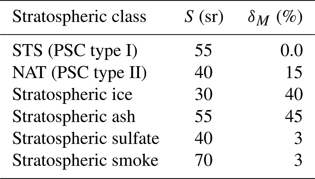
2.3.5 Stratospheric-layer classification
Layers whose tops are above the tropopause level are subjected to a similar classification procedure involving thresholds on the attenuated backscatter and examining the layer depolarisation ratio and lidar ratio. The following default stratospheric classes have been defined (see Table 2).
2.4 Class smoothing and outputs
After the classification procedures have been applied to all the layers in each column, a final additional step is performed. For areas classified as being weak targets, e.g. thin ice cloud and aerosols, a smoothing filter at height and along-track is applied to the classification in order to increase the homogeneity of the classification and remove any small gaps. The filtering performed is based on a hybrid-median (HM) filtering technique, which is very effective in removing single noise events and filling gaps. Since the HM technique uses only median values, there are no smoothing edge effects.
In the case of classifications, an integer-based scale is used where individual values will have very different meanings. The median of an array of values may not necessarily reflect the most common target and cannot be used in this case. To overcome this, the target type's frequency of occurrence is calculated, and the highest target type occurrences (modes) are used instead of the median.
In Fig. 4, the flow diagram of the weak target smoothing is shown. For the entire orbit, a box of size nhor×3 is defined around each pixel. Within each box, the highest particle type occurrence is calculated. The local position can only be updated when the initial classification is clear sky or ice cloud or when it contains one of the aerosol types. In those cases when a pixel is switched to clear sky while there is a confidently retrieved particle extinction or when a pixel is switched to ice while the temperature is greater than 0 ∘C, the original classification is retained. Any pixels which can not be defined due to the procedure and which were previously clear sky are set to unknown.
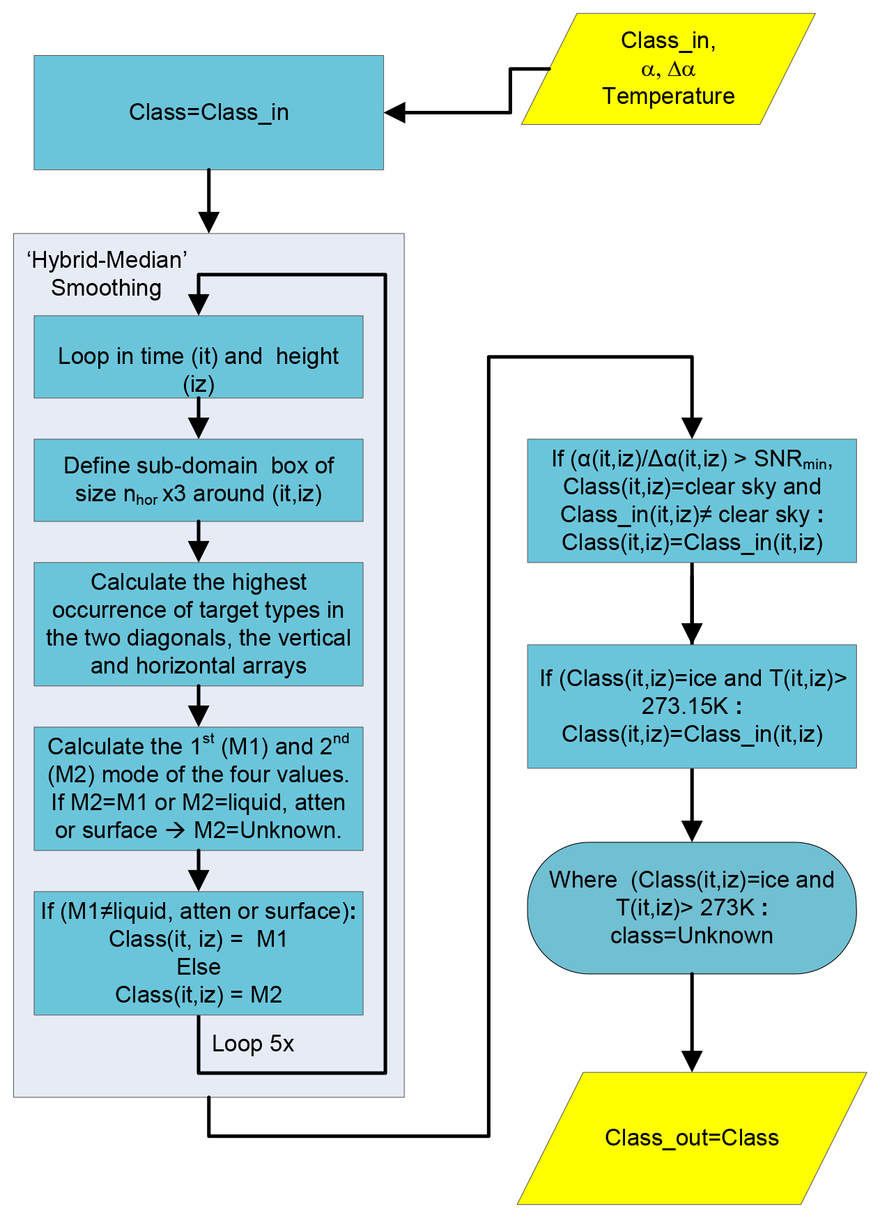
Figure 4Flow diagram depicting the smoothing strategy of A-TC weak targets to increase homogeneity. The same strategy is performed for the entire grid five times (large box) where any local weak target type (ice or aerosol type) is updated to the type with the highest occurrence in a nhor×3 local sub-domain. The final three boxes perform checks to ensure that no obvious misclassifications have been made.
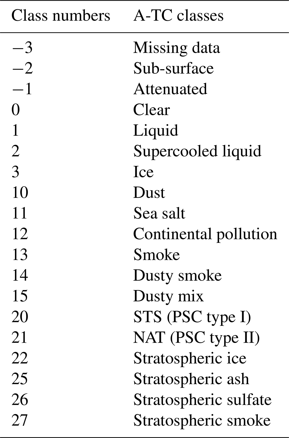
The classifications yielded by A-TC, and their numerical values as encoded in the target classification variable, are shown in Table 3. A-TC outputs are produced for three horizontal resolutions. These correspond to the high, low and medium resolutions used by the A-EBD algorithm component of the A-PRO processor (Donovan et al., 2023b). Variables in the AC-TC product also correspond to these three resolutions (see Sect. 4). The table contains information not directly related to the classification procedure described here but rather propagated from the ATLID-featuremask (A-FM; van Zadelhoff et al., 2023b) and A-PRO (e.g. attenuated regions). The information is provided on a pixel-by-pixel basis and not on a layer-by-layer basis (though the per-column layering used is available in A-PRO outputs).
Finally, it should be noted that, for the high-, medium- and low-resolution products, the layering structure is the same for each version, but the horizontal scale varies. High resolution corresponds to about 1 km along-track; medium is, by default, is 50 km; while low corresponds to 150 km. The medium and low horizontal scales are configurable with A-PRO.
The range-resolved CPR radar reflectivity and mean Doppler velocity measurements provide unprecedented information about the vertical and horizontal structure of clouds and precipitation. The CPR observations, along with information about the cloud and precipitation altitude, remove word-texture thickness, and temperature is used in the identification of the different types of clouds and precipitation and hydrometeor types. Such a CPR-based target classification is very important for the evaluation of global and regional numerical models. There is considerable heritage in target classification algorithms using range-resolved radar and lidar observations for both surface-based (e.g. Illingworth et al., 2007; Kollias et al., 2009) and space-based systems (Marchand et al., 2008; Mace and Zhang, 2014; Ceccaldi et al., 2013; Delanoë and Hogan, 2010).
The EarthCARE CPR target classification (C-TC) is based on a decision tree algorithm with fixed rules, and it is designed to work as a stand-alone product. The main steps of the detailed C-TC classification procedure are depicted in Fig. 5. In order to facilitate its use and integration in the synergistic target classification, we have adopted similar target classification definitions and names. Doppler velocity classification provides additional information about the quality or applicability of the mean Doppler velocity measurements for the cloud and precipitation retrieval algorithms.
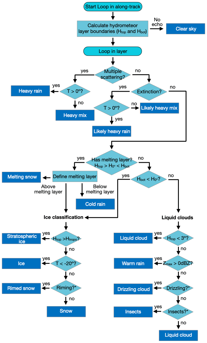
Figure 5Schematic of the C-TC detailed-classification procedure. (*) Refer to the text for a detailed explanation.
The first step in the C-TC algorithm is the objective determination of the boundaries (echo top and echo base) of the different hydrometeor layers observed in the atmospheric column sampled by the CPR. The output of the CPR featuremask algorithm (C-FMR; Kollias et al., 2022) is used to estimate the time series of the hydrometeor layer boundaries. We refer to these boundaries as hydrometeor layer boundaries and not cloud layer boundaries, since it is challenging when using only CPR measurements to discriminate between cloud and light precipitation in liquid clouds, and there is no clear definition of ice cloud versus precipitating ice. Thus, the reported boundaries report the vertical extent of both cloud and precipitation type hydrometeors in the atmospheric column.
The second step in the C-TC algorithm is the determination of the presence of the radar signature of the melting layer. The melting-layer detection algorithm is applied in hydrometeor layers with tops and boundary heights below and above the 0 ∘C wet-bulb isotherm. The methodology is based on the work of Geerts and Dawei (2004), with some additional criteria added and existing thresholds modified. First, local reflectivity maxima Zmax close to the freezing level (1 km above and 1 km below) are identified. These maxima are considered to be candidates for the bright band if (a) the reflectivity 500 m below (Zb) exceeds the reflectivity 500 m above (Za), (b) the local maximum reflectivity exceeds Za by at least 2.5 dB, and (c) the velocity gradient in a layer 500 m above the 0 ∘C wet-bulb isotherm and 500 m below the level of Zmax exceeds the threshold of 2 m s−1 km−1. If these conditions are satisfied, the level of Zmax represents the level where melting starts. Then the level of maximal value of Doppler velocity (z(Vdmax)) is determined in the layer between z(Zmax) and z(Zmax−800 m). The bottom of the melting layer is determined as the level above the z(Vdmax) where the absolute value of the vertical gradient of the Doppler velocity is minimal.
The third step is the cloud and precipitation type classification (Table 4). Using the estimated hydrometeor layer boundaries, the X-MET (Eisinger et al., 2023) temperature, melting-layer height boundaries, radar reflectivity and mean Doppler velocity, the rules described later in Sect. 3 are employed for the determination of different cloud and precipitation types.
3.1 Clear skies
If the C-FMR hydrometeor featuremask reports no significant meteorological origin echoes in the atmospheric column, then the atmospheric column is declared to be clear (at least with respect to the sensitivity of the CPR).
3.2 Ice classification
A layer is identified as ice if the base of the layer is above the height of the 0 ∘ wet-bulb isotherm. At temperatures lower than (homogeneous-ice-freezing regime), all CPR echoes are classified as ice clouds. At temperatures warmer than −20 ∘C, the following two additional solid precipitation categories are allowed: snow and rimed snow.
The following conditions have to be satisfied to identify the presence of a snow layer in each profile: 75 % of the pixels need to have a reflectivity and a Doppler velocity higher than −15 dBZ and 0.4 m s−1, respectively. It is important to note that the hydrometeor sedimentation Doppler velocities are first adjusted for density effects by referencing them to standard surface level conditions before they are used as input to the C-TC algorithm an indicator. The depth of the layer has to be greater than 300 m to be identified as snow.
In a detected snow layer at temperatures higher than −15 ∘C, in the presence of larger particles, a rapid increase in terms of Doppler velocity above 1 m s−1 (referenced in relation to surface level conditions) is treated as the signature of riming. Since rimed snow and snow aggregates can have similar values of radar reflectivity, the localisation of the rimed snow layer is based mainly on the vertical structure of Doppler velocity. The minimal vertical gradient of integrated Doppler velocity required to identify the riming is 0.5 m s−1 km−1. This velocity increase downwards cannot be accompanied by a reduction in radar reflectivity. If one or more of the ice layer boundaries is above the height of the tropopause, it is characterised as stratospheric ice cloud.
3.3 Liquid clouds
If the top of the hydrometeor layer is below the height of the −3 ∘C isotherm, then the layer (and all the layers below it) is classified as liquid cloud.
Liquid layers are further classified as non-precipitating (drizzle-free and slightly drizzling clouds) and liquid precipitating clouds (heavy drizzle and rain). Radar reflectivity has been traditionally used (in the absence of other complementary measurements such as lidar observations) to distinguish precipitating from non-precipitating liquid clouds (Kollias et al., 2011). Different radar reflectivity thresholds have been proposed in the literature, with values ranging between −25 and 0 dBZ (Frisch et al., 1995; Mace and Sassen, 2000; Krasnov and Russchenberg, 2005; Liu et al., 2008; Zhu et al., 2022). A general conclusion is that there is no unique threshold in any of the parameters that can be used to do the separation between drizzle-free and drizzling clouds. There is, rather, a probability of precipitation that increases within a range of reflectivity, a range of liquid water path (LWP) or a range of Doppler velocity. In addition, as suggested by Fox and Illingworth (1997) and Mace and Sassen (2000), the vertical structure of the radar reflectivity profile can be used in the estimation of the probability of the drizzle-free occurrence. In particular, a steady increase with altitude is a good indicator of drizzle-free conditions. In C-TC, the identification of drizzling clouds is based on the following two parameters: a CPR reflectivity threshold and the CPR-derived apparent cloud thickness (H) determined as the liquid cloud vertical extension. The CPR reflectivity threshold for detecting the presence of drizzle is set to −20 dBZ. This is based on the aforementioned literature and the impact of the CPR sampling volume on the reported radar reflectivity. If the maximum reflectivity Zmax exceeds −11 dBZ, then the presence of drizzle is assumed to be almost certain. On the other hand, if the profile maximum reflectivity Zmax is below −29 dBZ, then the presence of drizzle is ruled out. Thus, the overlap of possible drizzle or cloud-only conditions exists across the Zmax range of values between −29 and −11 dBZ. In this Zmax range, if the thickness H of the radar column exceeds 700 m, then the profile is classified as certainly drizzling. On the other hand, if the thickness H is lower than 400 m, i.e. three CPR range gates or less, the profile is identified as cloud-only drizzling. The CPR profiles that have thicknesses between 400 and 700 m and Zmax between −29 and −11 dBZ correspond to the overlapping-conditions regime.
In addition to the distinction between non-precipitating liquid clouds and drizzle-containing liquid clouds, we further classify liquid clouds as warm rain if Zmax in the column exceeds 0 dBZ.
3.4 Cold rain and insects
If a hydrometeor layer has a base below the height of the 0 ∘C wet-bulb isotherm and a top above the height of the −3 ∘C isotherm, then the layer below 0 ∘C is classified as cold rain (this could be rain originating from melting ice) and ice (ice cloud, snow or rimed snow) above the top of the melting layer. The procedure described in the ice clouds section is then applied to characterise the ice layer above the melting layer. If a melting layer was detected, then melting snow will overwrite the cold-rain pixels inside of the melting layer.
Over land and when the air temperature is not lower than 15 ∘C, there is a significant record of observations from profiling millimetre-wavelength radars (Luke et al., 2008; Chandra et al., 2013; Kollias et al., 2014; Lamer and Kollias, 2015) that suggest that most of the radar echoes are from deep insect layers. Furthermore, because of non-Rayleigh scattering, the insect radar reflectivity is typically below −20 dBZ. Based on the above information, all CPR echoes over land and below 3 km altitude with reflectivity lower than −20 dBZ and temperatures not lower than 15 ∘C are classified as insects.
3.5 Multiple scattering and extinction
Following Battaglia et al. (2011), multiple-scattering (MS) effects are detected computing the top-down integral of reflectivity I(z) values above a certain threshold Zthres. MS is likely to be encountered below the height H(MS) where I(z) exceeds a critical value Zthres. For the EarthCARE CPR technical specifications, the best statistical match to identify MS is achieved when Zthres is selected to be equal to 12 dBZ and when I(z) exceeds 41 dBZint. All values below the H(MS) level are classified as heavy rain or heavy mixed-phased precipitation if temperatures are below 0 ∘C.
When MS is not detected but the CPR does not provide measurements of the surface return echo, it is most likely because the receiver signal is completely saturated due to attenuation. All values between the ground surface and the first detected layer are classified as likely heavy rain or likely heavy mixed-phased precipitation if temperatures are below 0 ∘C.
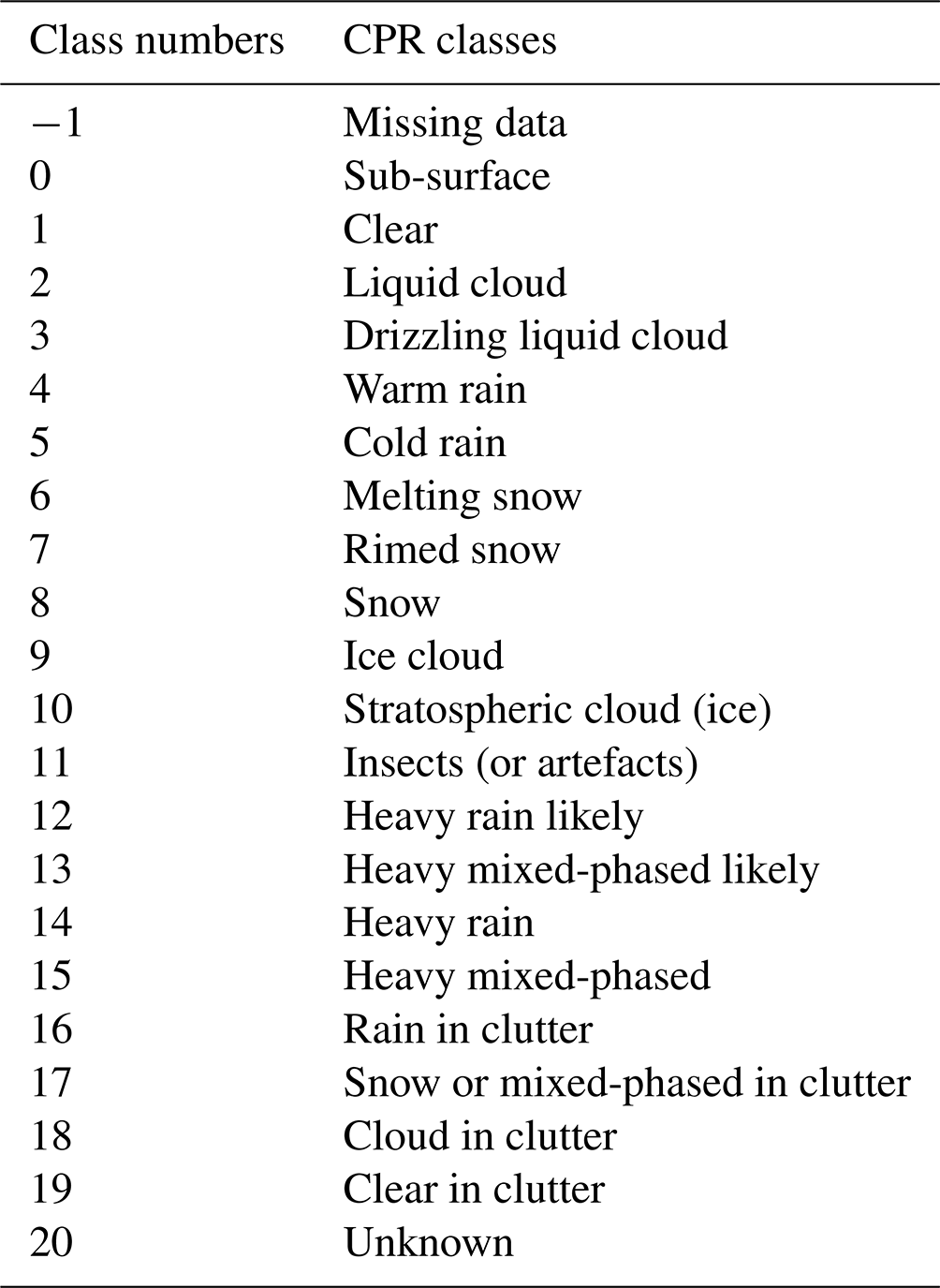
The values and descriptions of the CPR target classification are given in Table 4.
AC-TC is a synergistic product that combines ATLID and CPR observations and therefore provides information on horizontally and vertically resolved structures of different atmospheric targets (aerosols, clouds, rains, etc.). It takes up the essential information from the two instruments with the advantage of removing any ambiguity regarding the nature of the atmospheric targets thanks to the complementarity of the instrumental responses (see Sect. 4.1). This product is the result of prior knowledge acquired during the development and maintenance of DARDAR-MASK (Ceccaldi et al., 2013; Delanoë and Hogan, 2010, https://www.icare.univ-lille.fr/dardar/documentation-dardar-mask/, last access: 20 May 2023), which combines CloudSat and CALIPSO measurements. The AC-TC product will, however, incorporate the improvements in target classification provided by EarthCARE's new high-spectral-resolution lidar and Doppler radar capabilities, as shown below.
The AC-TC processor assigns all pixels in an EarthCARE granule to the classifications defined in Table 5 by merging A-TC and C-TC products according to a synergistic decision matrix (Fig. 6). Some preprocessing is needed for the input products so that the atmospheric profile obtained from each instrument has the same altitude sampling. ATLID and synergistic data products use a common joint standard grid (X-JSG; Eisinger et al., 2023), which is defined by the vertical resolution of ATLID (≈103 m) and along-track according to CPR (1 km, corresponding to ≈2 radar pixels), with an across-track sampling size of 1 km. A-TC and C-TC are defined on different vertical grids; ATLID data are on the X-JSG grid by definition, while C-TC is on the native-radar-sampling grid. Both vertical grids have an approximate 100 m sampling. The C-TC variables are regridded onto the X-JSG vertical grid using a nearest-neighbour approach, which will result in relatively small vertical displacement (a maximum 50 m offset) that is not expected to result in any noticeable issues. The top of the cloud will be defined by lidar signals due to its higher vertical resolution.
Table 5Definition of AC-target classes linked to the lidar–radar properties involved.
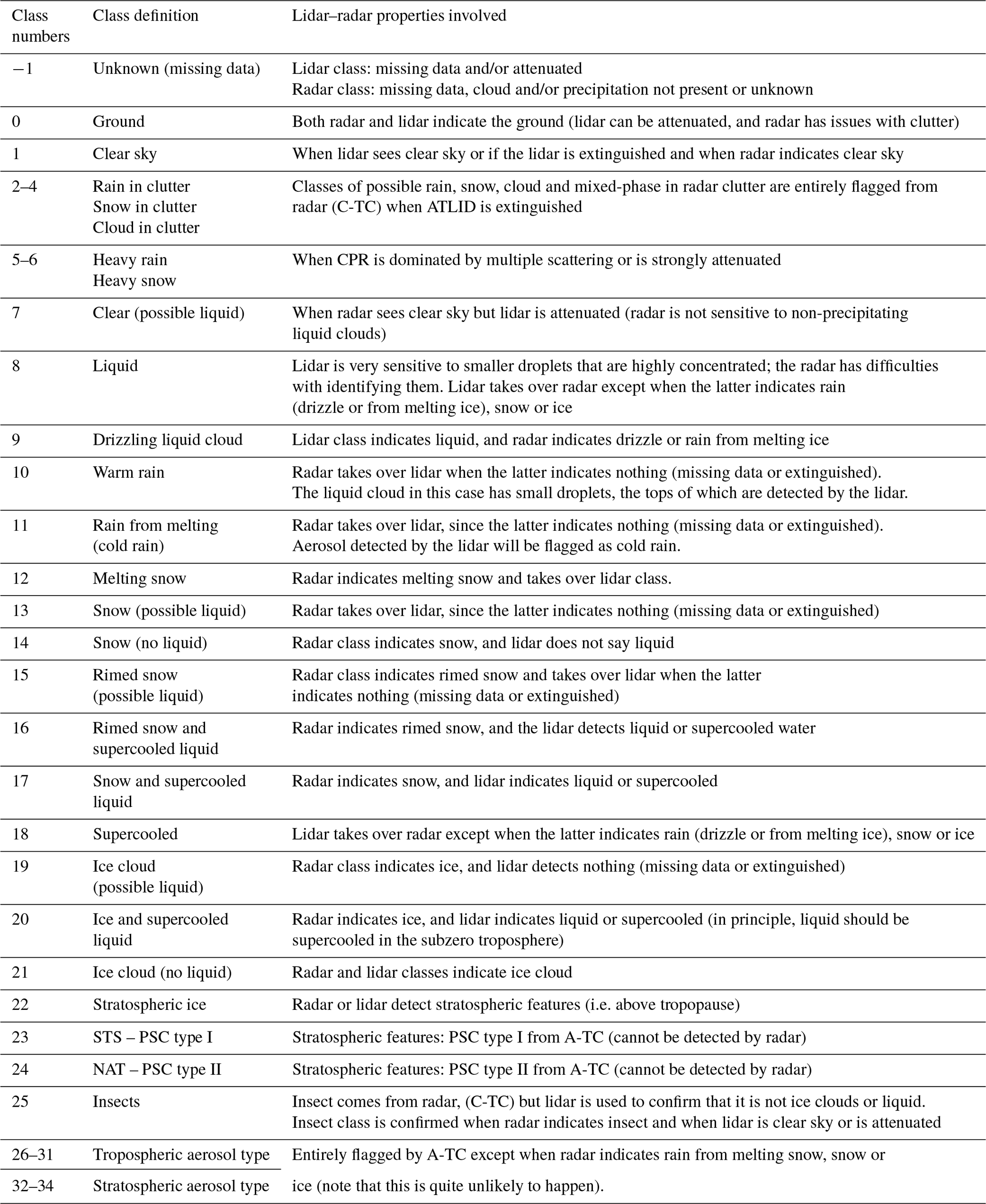
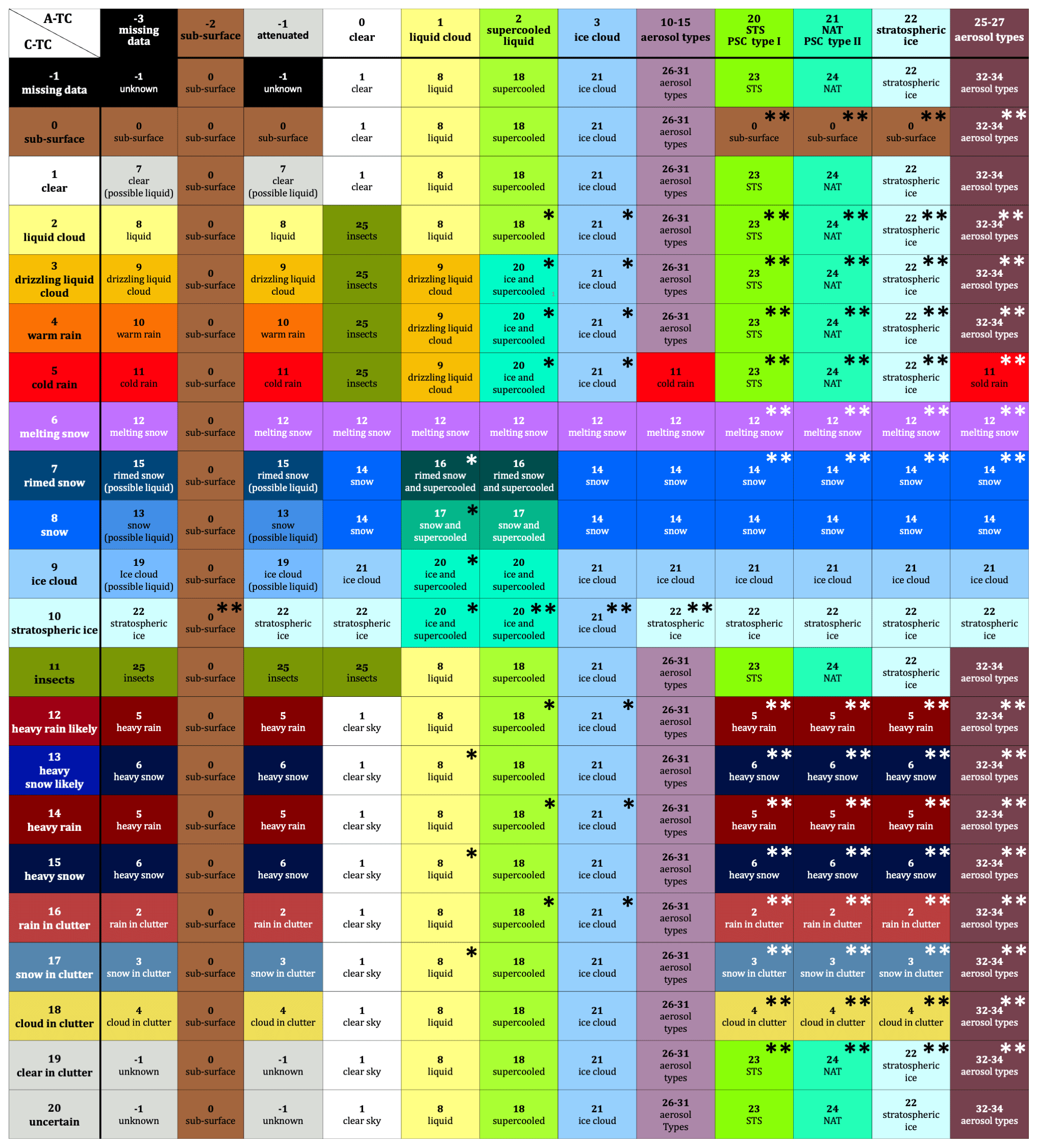
Figure 6The AC-TC decision matrix assigning the synergistic classification at each pixel based on A-TC classes (horizontal) and C-TC classes (vertical). Synergistic classifications are mostly assigned in ice and mixed-phase clouds; in most other situations, one instrument or another takes precedence. The decision matrix includes all combinations, including those that are physically unlikely or impossible except due to an error in the input products. The decision matrix assigns a common-sense interpretation to these conflicts, but occurrences of these instances will be tracked for the purposes of verification and quality assurance. Two such conflicts are denoted with asterisks; * indicates disagreements about temperature or thermodynamic phase, while indicates significant disagreement about altitude.
4.1 Decision matrix
The radar and lidar provide independent information of the same probed atmospheric regions in the microwave and optical domains, respectively. Radar can penetrate thick ice clouds and precipitation, while lidar can detect aerosols, ice clouds and liquid clouds. Target detection will then be based on the combination of signals from both instruments and will follow a decision tree. This process is described in this section. First of all, it is useful to recall the main information provided by the two instruments. The lidar retrieves information on the nature of hydrometeors thanks to the backscatter signals in the Mie channel, as well as their depolarisation. Strong Mie backscatter is the signature of either liquid clouds, of ice in high concentrations or of mixed-phase cloud. The radar reflectivity provides information on optically thick ice clouds and on larger precipitation particles (snow or rain). Radar measurements thus take precedence over lidar for the identification of rain, drizzle and snow. The parts of ice clouds detected by both instruments overlap at best, but neither instrument resolves the entire profile independently. These complementary properties of radar and lidar demonstrate the appeal of using a synergistic approach to produce a comprehensive classification of all hydrometeors and aerosols in the atmosphere. The AC-target classification is presented in Table 5, where the main instrumental properties according to which each class is defined are described in the third column. Each co-located pixel of the CPR and ATLID measurement profiles is assigned a class in Table 5 according to the probing properties of the instruments, resulting in the decision matrix shown in Fig. 6. Some instrument detection properties useful for filling the decision matrix summarised in Table 5 are recalled in the following Sect. 4.2 to 4.7
4.2 Liquid cloud
The detection of liquid cloud is challenging for CPR but is possible depending on the sensitivity and the presence of drizzle. On the other hand, the lidar is very sensitive to the highly concentrated small droplets and shows a very strong signal return. AC-TC distinguishes the following two types of liquid cloud: warm and supercooled. Supercooled liquid identified in A-TC can be co-located with ice clouds, snow and rimed snow in C-TC, in which case AC-TC returns a mixed-phase classification.
4.3 Ice cloud, snow, rimed snow and melting ice
Ice clouds can be detected by both radar and lidar. CPR will not be able to detect the optically thinnest ice clouds. As a result, when ice is identified either by A-TC or C-TC, AC-TC reports an ice or snow class. Furthermore, the magnitude and vertical structure of CPR's mean Doppler velocity measurement are used to distinguish between ice clouds, snow and rimed snow (see Sect. 3). Melting ice corresponds to the area where snowflakes melt and are converted into raindrops. This information comes from C-TC. Complementary information is used to classify mixed-phase cloud when A-TC indicates the presence of supercooled liquid and when C-TC identifies ice cloud, snow or rimed snow. When ATLID is extinguished, the C-TC classification is used, but the possible presence of liquid cloud is reflected in the target classification (i.e. liquid possible).
4.4 Rain
The above set of rules mainly distinguishes the different types of clouds but so far neglects precipitation and its determination. There are two types of rain, namely cold rain and warm rain, both referring to the types of clouds in which the rain originates. Rain assignment will therefore depend on C-TC only. In the warm-rain case, it is relatively straightforward; the liquid water cloud itself has small droplets, for which the top is detected by the lidar if the beam is not extinguished by higher cloud layers. The radar will start to detect the droplets when they grow into drizzle and raindrops. Cold rain originates from the melting of snow.
4.5 Aerosol
Due to their small size, aerosols cannot be detected by radar. Therefore the aerosol class only depends on lidar measurements, and the radar flag should indicate clear sky (or unknown or clutter). If the radar detects an echo, it is important to check the confidence level in the lidar flag – for example, if the radar detects ice cloud, the pixel will be treated as such. In all other cases, when an A-TC aerosol classification is available, AC-TC will inherit the corresponding aerosol type from A-TC.
4.6 Insects
The detection of insects comes from the radar measurement (see Sect. 3.4) in the absence of lidar measurements which could confirm that the radar is detecting another hydrometeor classification. When the radar identifies insects and the lidar classification reports clear sky (or attenuated), the pixel is maintained to the insect class. This target classification is rarely made by CloudSat; however, the increased sensitivity of the EarthCARE CPR might give rise to increased detection of insects. In the case of insects above clouds, the lidar signals should detect no Mie signals and no decrease in the Rayleigh signals. Also, the smearing of the radar signal due to the long pulse length has to be taken into account before assigning the insect flag to the radar return. In general, more than one pixel is needed to be sure that insects are detected. In principle, insect detection is considered if A-TC indicates clear sky and C-TC indicates liquid cloud or light rain. Note that insects can be erroneously detected if the lidar signal is very weak – for example, due to contamination by photons from the sun.
4.7 Ground or clear-sky detection and the unknown or clutter situation
The ground or sub-surface classification is assigned below the level at which the lidar detects a surface return. It is also assigned when the radar sees the ground and the lidar is attenuated or has data issues (missing data).
Clear sky is identified when lidar and radar both indicate clear sky. In the case where the lidar is extinguished (fully attenuated) and the radar indicates clear sky, the classification includes the possibility of liquid cloud targets.
The unknown classification occurs when there is no reliable information from both radar and lidar.
Concerning the radar surface clutter region, it essentially relies on a specific processing of the radar reflectivity signal coming from zones assumed to be close to the ground. The C-TC classes resulting from this processing will be taken as such for this region.
Simulated data is needed to test the methods and associated processors developed to calculate A-TC, C-TC and AC-TC. Three simulated scenes covering approximately one-eighth of an EarthCARE orbit (5000 km) were therefore developed, namely the scenes of Halifax (covering the mid-latitudes of the Northern Hemisphere passing over eastern Canada, the western Atlantic Ocean and the Caribbean), Baja (which crosses western Canada, the United States and the Baja Peninsula) and Hawaii (above the central Pacific Ocean beginning near Hawaii; Donovan et al., 2023a). AC-TC was also applied to the Baja and Hawaii scenes, but only the results for the Halifax scene are presented in this section. The results for the other two scenes are presented in a broader evaluation context in Mason et al. (2022). The Halifax scene is one of the three test scenes developed based on high-resolution cloud-resolving model data from the Environment and Climate Change Canada (ECCC) GEM (Global Environmental Multiscale) model merged with CAMS (Copernicus Atmosphere Monitoring Service) aerosol data. The construction of the model fields is described in detail in Qu et al. (2022). The radiative transfer and instrument simulation methods applied in order to produce EarthCARE ATLID, CPR, MSI and BBR (Wehr et al., 2023) simulated L1 data are described in Donovan et al. (2023a). The ECCC model scenes were produced to facilitate the development and testing of the EarthCARE processors implemented in the Payload Data Ground Segment (PDGS). Figures 7 and 8 show some sample true model fields along with simulated L1 ATLID and CPR data for the Halifax scene. In particular, the aerosol–cloud mass and effective radius extracted from the scene are shown along with the ATLID Mie, Rayleigh and cross-polar L1 attenuated backscatters, and the radar reflectivity. Even at the level of the L1 data, the complementarity of the lidar and radar fields is apparent. For example, the radar is not attenuated by the extensive clouds present near the centre of the scene. On the other hand, the lidar readily detects the aerosol fields and (supercooled-)liquid water clouds that are largely missed by the radar.
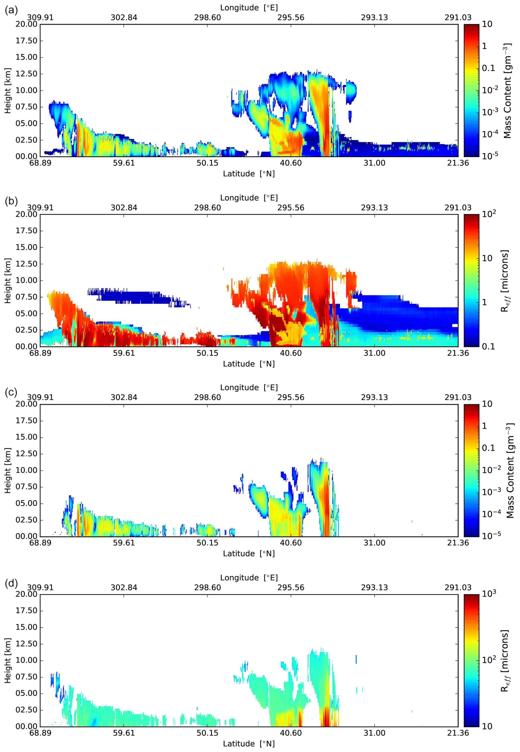
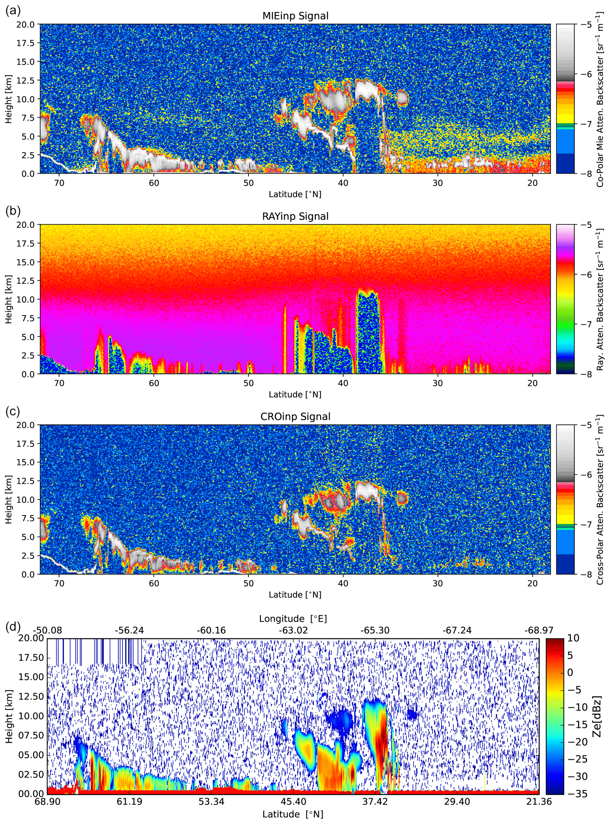
Figure 8In order from top to bottom: simulated ATLID cross-talk-corrected attenuated backscatters and simulated CPR radar reflectivity factor for the Halifax scene. Note that the stripy area in the top-left section of the radar reflectively panel corresponds to an area above the PRF-determined radar maximum altitude for that section of the orbit.
The AC-TC processor will produce the synergistic target classification product that takes the A-TC and C-TC products as inputs. Figure 9a and b show the ATLID and CPR target classifications corresponding to the ECCC Halifax scene (Donovan et al., 2023a).
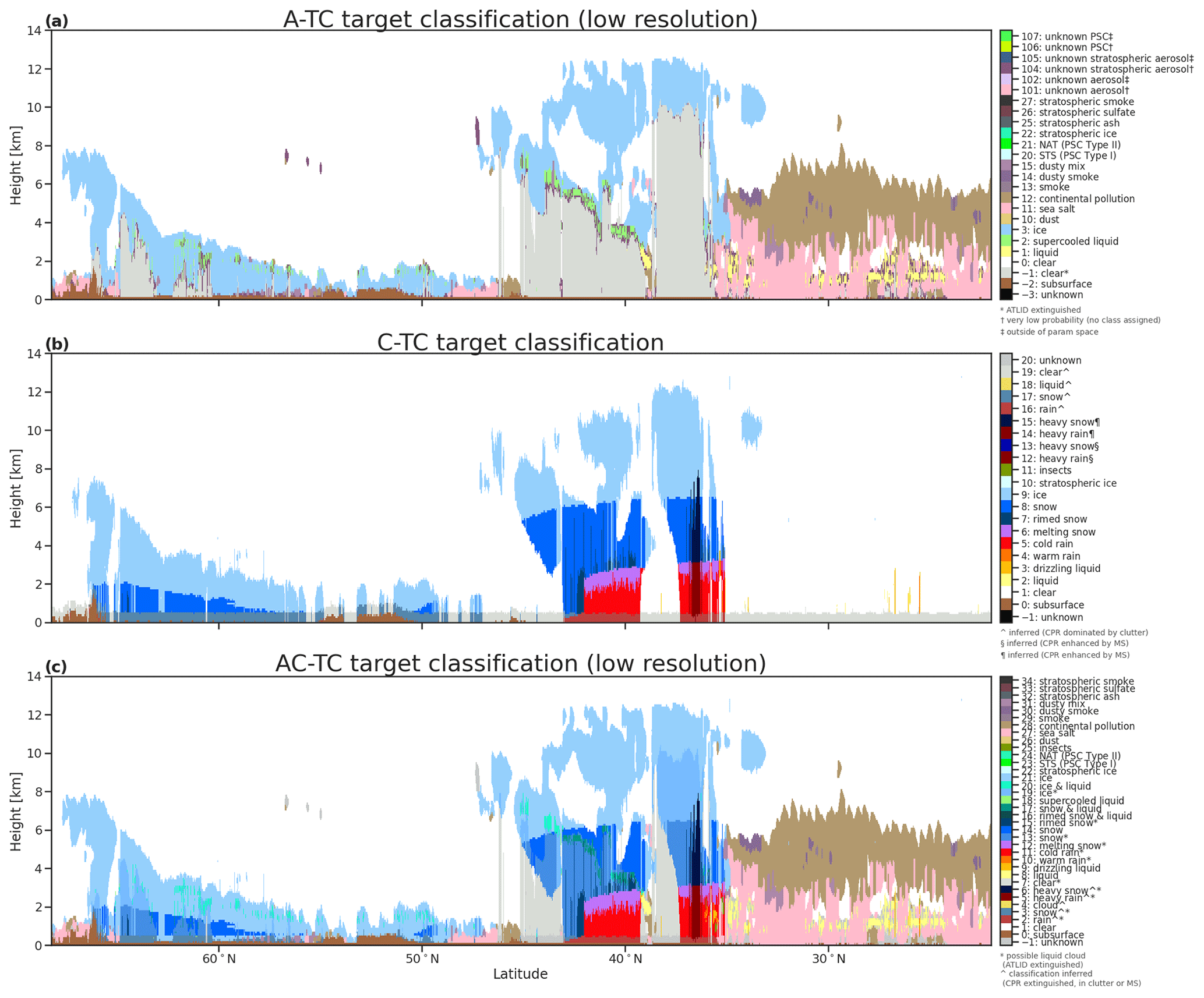
The A-TC algorithm is described in Sect. 2. Here, the ice clouds are, in general, well seen and classified by A-TC (Fig. 9a). As A-TC can only classify the targets up to the point where the lidar signal is attenuated, a substantial area marked as attenuated exists between about 35 and 45∘ N and is unclassified. Extensive supercooled liquid layers are also present in this region. The broken warm liquid clouds south of about 35∘ N are, in general, well detected by the lidar. The aerosol layers present south of about 35∘ N are broadly well classified by the A-TC; however, there are some areas of misclassification present here and there (the true classification should be continental pollution above about 2.5 km and sea salt below). Here, both aerosol types are non-depolarising so that the aerosol type is based on the layering determination and the lidar–ratio estimate from A-PRO (see Donovan et al., 2023b).
C-TC is based on the methodology discussed in Sect. 3. In the high-latitude (50 to 70∘ N) part of the Halifax scene, C-TC correctly identifies the echoes containing ice cloud and snow (see Fig. 9b). This classification is based on the temperature of the layer, while the separation between ice cloud and snow is based on temperature, radar reflectivity and Doppler velocity thresholds. At lower latitudes (39 to 43∘ N), a large-scale frontal precipitation system is observed, and a transition from snow to cold rain is correctly captured by C-TC. After a brief snow period, the hydrometeor layer base is warmer than 0 ∘C.
Using the CPR radar reflectivity and mean Doppler velocity and the X-MET based height of the 0 ∘C, the C-TC identifies the presence of melting snow. Above the melting layer, ice and snow hydrometeors are detected, and below the melting layer, cold rain is observed. Finally, at even lower latitudes (35 to 37∘ N), another mesoscale precipitation system is observed with a convective core. In the convective core, C-TC identifies the presence of rimed particles in the upper part of the layer and cold rain below. Overall, C-TC accurately captures most of the important features of the precipitation systems in the Halifax scene.
The AC-target classification is shown in Fig. 9c. The version shown is the low-resolution version based on the A-target classification with a long along-track integration length (see Sect. 2.4), which is reflected in the low-resolution AC-target classification. Medium- and high-resolution AC-TC target classification variables are also included in AC-TC product as well as A-TC target classification (all resolutions) and C-TC target classification variables. Figure 9c shows that the resolved structures resemble the union of those classified by the two instruments in Fig. 9a and b; specifically, ice cloud tops detected by A-TC expand upon the ice clouds resolved by C-TC; the large parts of the scene where ATLID is extinguished are filled in by the detection of snow, melting snow and rain in C-TC; and where C-TC reported clear skies, A-TC often provides the detection of aerosols layers. Synergistic classifications are possible where A-TC detects a layer of supercooled liquid and where C-TC detects ice clouds and snow; here, AC-TC is able to diagnose a range of mixed-phase classifications.
The AC-TC product, which incorporates A-TC at all resolutions and C-TC, can, on its own, be used to derive important statistics regarding the spatiotemporal distributions and structures of aerosols, clouds and precipitation, as well as their properties and thermodynamic phases (e.g. Mioche et al., 2015, 2017; Vérèmes et al., 2019; Listowski et al., 2019, 2020). It also facilitates the application of the ACM-CAP synergistic retrieval algorithm (Mason et al., 2022). Principally, it identifies the nature of the targets in each pixel and highlights classifications that are uncertain or ambiguous, thereby informing subsequent algorithms where they should perform a retrieval (e.g. an ice cloud algorithm would only be applied to pixels containing ice cloud) and in some cases the confidence that they should assign to the observations at each pixel (e.g. when the lidar is extinguished in ice cloud, so the presence of mixed-phase cloud cannot be ruled out). In addition, AC-TC will be ideal for deriving cloud fraction and cloud overlap on arbitrary model-type grids. It is therefore important to validate the target classification products using simulated scenes for which the expected result is known, as is the case with the Halifax scene of Fig. 9c.
The three test scenes (see Sect. 5) and the numerical model quantities used to create them (Sect. 5 and Qu et al., 2022) can be used to carry out an omniscient evaluation of the target classifications. In this section, we quantify the degree to which the spatial distributions of broad classes of hydrometeors or aerosols are accurately represented by the lidar, radar and synergistic target classifications. The capability of a target classification to recover the distribution of aerosols, clouds and precipitation can be considered volumetrically, which prioritises the optically thin or light-precipitation features that are often critical to radiation and energy budgets, or in a mass-weighted sense to focus on the total mass contents. The broad classes considered here are ice clouds and snow (Sect. 6.1), liquid clouds (Sect. 6.2), rain (Sect. 6.3), and aerosols (Sect. 6.4). The verification of each product compares the target classification against the mass content of water or aerosol species in the numerical model and assigns each pixel the status of hit (correct identification), miss (incorrectly classified as clear or another class, where a target exists in the model), false positive (a classification is made where no target exists in the model) or correct negative (correctly classified as clear or another class) after masking for sub-surface pixels and regions where the instrument is extinguished. For C-TC and AC-TC, additional statuses are included for correct inference and false inference in pixels where no detection is made due to surface clutter, attenuation or multiple scattering of the radar beam but where it may be possible to infer the presence of precipitation contiguous with the pixels above. These inferences are not made unilaterally within the target classification but are an interpretation of the classes that encode information about the limitations of the active instruments. The evaluation will show that, in some cases, these choices will result in some amount of false inferences, even while they improve the total fraction of hydrometeors that are accurately resolved.
While the Halifax scene is used to illustrate the evaluation of the target classifications, Fig. 10 provides the percentages of each class of hydrometeors that are correctly identified across all three test scenes (Halifax, Baja and Hawaii) by volume (fraction of pixels containing each constituent) and by mass content. The stacked bar charts indicate the fraction of each class that is undetected (i.e. reported as clear sky), accurately detected, inferred (i.e. may be contextually likely, such as in contiguous regions of surface clutter or within convective cores) or obscured (i.e. another classification is made or the instrument is extinguished, such as in the case of aerosols that are not detected in the presence of hydrometeors). This evaluation gives an indication of the fraction of targets that may be resolved by EarthCARE's active instruments within the limitations of their sensitivities and viewing geometry; however, we note that the three test scenes have not been designed to be statistically representative of the entire atmosphere, so this evaluation should not be interpreted as quantifying the global or long-term performance of EarthCARE's target classification products.
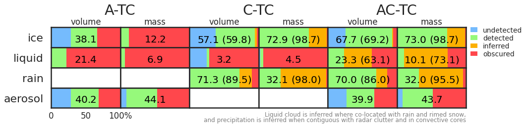
Figure 10Fractions of hydrometeors or aerosols correctly identified by A-TC, C-TC and AC-TC over the three simulated test scenes. For A-TC and AC-TC, the low-resolution version of the target classification is used. The volume fraction refers to the percentage of pixels on the joint standard grid that are correctly identified by the target classification as containing the constituent in question. The mass fraction is calculated as the percentage of the total water or aerosol mass content within correctly identified volumes, where the true mass content is defined by the numerical model fields from which the scenes are created. Values in parentheses indicate the total fraction including inferred classifications.
6.1 Ice clouds and snow
The synergy of radar and lidar is greatest in ice clouds and snow, which are well sampled by both instruments.
ATLID detects (Fig. 11a) most cloud top features, with the exception of very optically thin cloud edges. The difference between the volumetric and mass-weighted fractions detected in A-TC (Fig. 10) shows that around one-third of pixels containing some ice are undetected by ATLID, but these make a negligible contribution to the total mass of ice and snow in the scene. The penetration of ATLID varies significantly through the scene, from 1 to 2 km in the high-latitude mixed-phase clouds and deep convective clouds to up to 8 km through layered parts of the scene around 40∘ N; the most rapid extinction of ATLID occurs in the presence of mixed-phase clouds. Roughly another one-third of pixels containing ice cloud and snow across the three scenes are obscured by the extinction of ATLID. Across the three scenes, these obscured pixels contain almost 90 % of the mass of ice and snow.
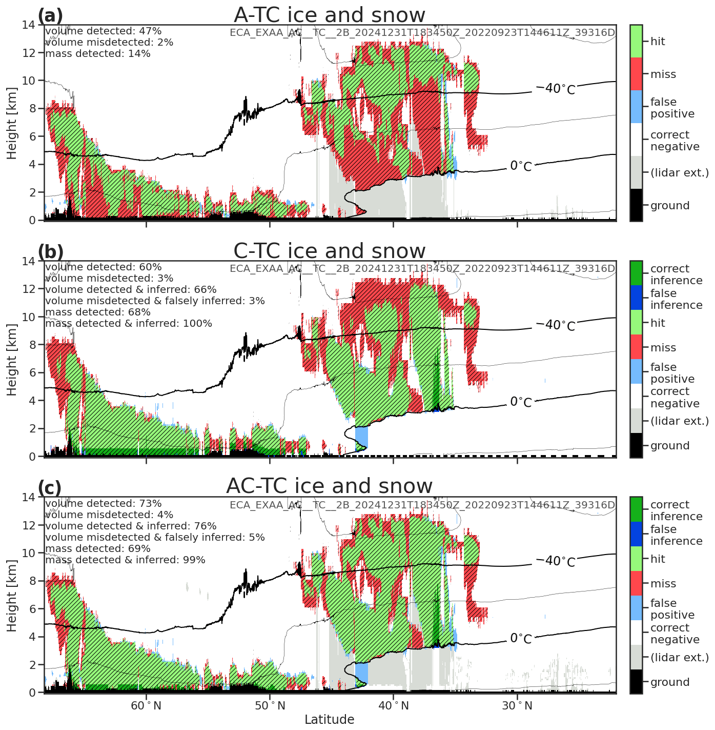
Figure 11An intercomparison of ATLID (a), CPR (b) and synergistic (c) detection of ice and snow target classifications for the Halifax scene. The volume fraction is calculated from the fraction of pixels detected compared to those containing any ice and snow in the GEM model after interpolation to the JSG (hatched areas). The mass fraction is based on the combined mass of ice cloud, snow, graupel and hail from the GEM model. The total fractions in C-TC and AC-TC include the inferred presence of ice and snow that cannot be detected directly by the instrument, such as within the ground clutter or where CPR is extinguished in deep convection. Atmospheric temperature contours from the model are overlaid. Grey shading indicates where each instrument is extinguished.
Despite its high sensitivity, the spatial coverage of ice cloud identified by C-TC (Fig. 11b) illustrates CPR's preferential sensitivity to larger particles. In the high-latitude mixed-phase cloud (50 to 63∘ N) and deep convective cloud (36 to 38∘ N) where ice growth and aggregation processes result in larger snowflakes, CPR resolves the cloud top nearly as accurately as ATLID; however, the high and optically thin clouds where particle sizes remain small (e.g. 38 to 48∘ N, where Fig. 7b shows ice clouds with effective radii less than 10 µm) contribute to the roughly 40 % of pixels containing ice that are not detected by CPR (Fig. 10). CPR is obscured by ground clutter in the lowest 0.5 km and is dominated by multiple scattering in the convective core (around 36∘ up to around 8 km). Across the three test scenes (Fig. 10), these obscured regions account for around 4 % of pixels but contain 25 % of the total mass of ice. Almost all of this ice and snow can be recovered because C-TC includes the likely identification of snow when contiguous with the surface clutter and of heavy precipitation within convective cores. This inference brings the coverage of CPR detection of ice clouds and snow to around 60 % by volume and more than 99 % by mass – however, the significant regions of cloud tops detected by ATLID and not by CPR are a reminder of the radiative importance of even very-low-water-content clouds.
The synergy of ATLID and CPR (Fig. 11c) allows for a more complete detection through the profile of ice clouds and snow (70 % by volume across the three scenes; Fig. 10) than is possible with either instrument alone. While the contribution of ATLID to detected ice clouds (around 10 % by volume) is around 0.1 % of the mass of ice and snow across the three scenes, the accurate detection of cloud tops from lidar is critical to EarthCARE's radiative closure. Ice at cloud edges or in virgae that goes undetected by both EarthCARE instruments represents around 26 % by volume and a negligible fraction by mass. Ultimately, AC-TC correctly identifies around 70 % of ice clouds and snow by volume, containing more than 99 % of the total ice water content, across the three simulated test scenes (Fig. 10).
6.2 Liquid
As noted in the descriptions of the single-instrument target classifications, CPR (Sect. 3) is most sensitive to the largest hydrometeors and rarely detects non-precipitating liquid cloud unless collocated with drizzle or rain. C-TC correctly identifies around 1 % of liquid clouds by volume in the Halifax scene (Fig. 12b) and around 3 % across all the test scenes (Fig. 10). We note that non-precipitating liquid clouds are not well represented in the present scenes, and the identification of liquid clouds in C-TC may be more effective in such cloud regimes. Conversely, A-TC (Sect. 2) capitalises on the strong signal returned from liquid clouds to detect the tops of liquid cloud layers, but its rapid extinction in a liquid results in no information about the physical depth of that layer or the possibility of layers below. The shallow layers of correctly identified liquid cloud in the Halifax scene (Fig. 12a) represent around 25 % of the volume of liquid clouds or around 7 % of total liquid water content in the scene; the grey shading in the figure shows the extinction of the instrument, while the hatching shows the true extent of liquid cloud in the model. Stated another way, across all three test scenes (Fig. 10) around 80 % of pixels containing liquid cloud and around 93 % of liquid water content are obscured by the extinction of the lidar signal. The synergistic classification of liquid cloud in AC-TC is therefore dominated by ATLID but includes possible-liquid-cloud classifications wherever ATLID is extinguished.
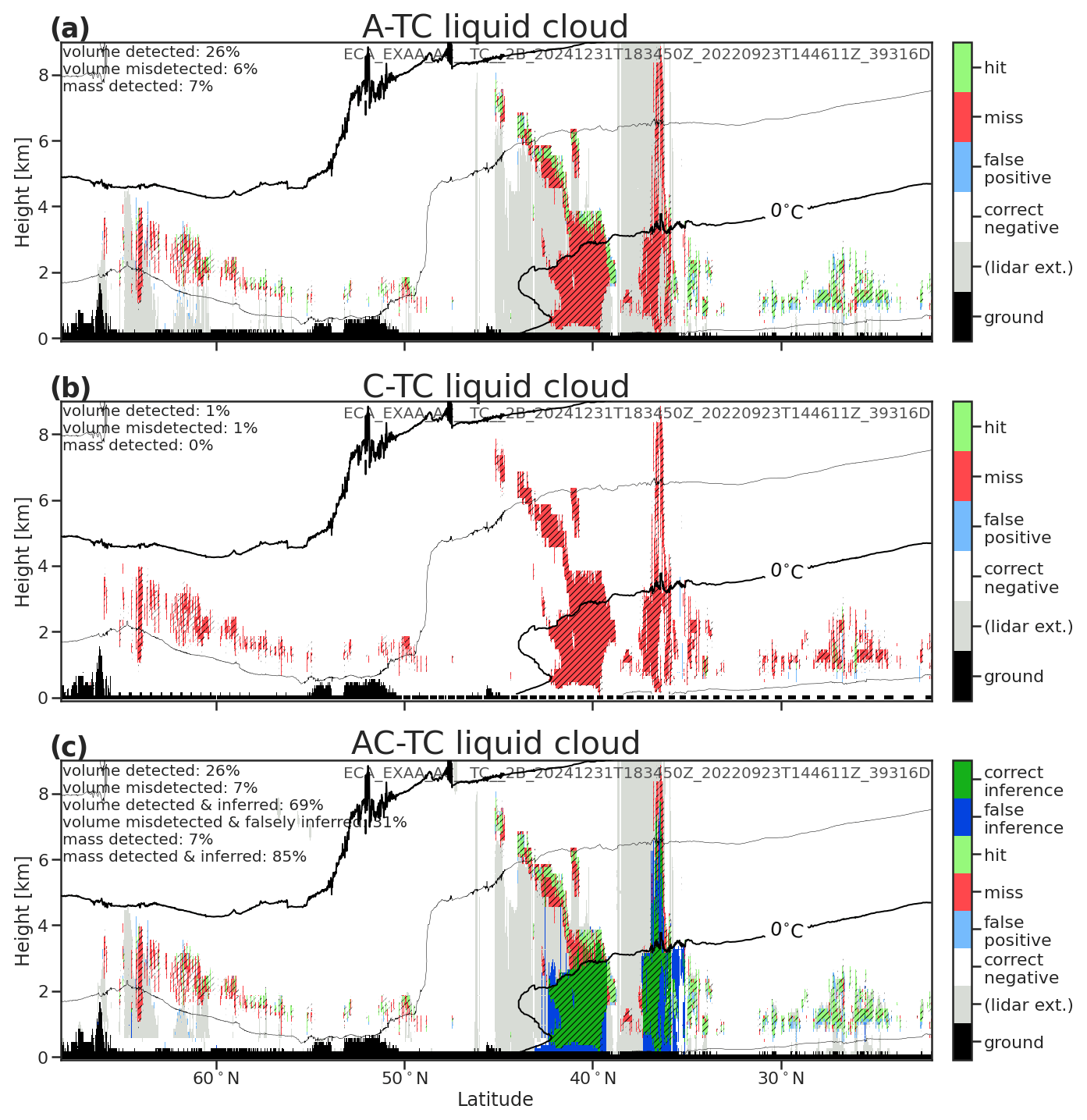
Figure 12An intercomparison of ATLID (a), CPR (b) and synergistic (c) detection of liquid target classifications for the Halifax scene. The volume fraction is calculated from the fraction of pixels detected compared to those containing any liquid cloud in the GEM model after interpolation to the JSG (hatched areas). The mass fraction is based on the mass of liquid cloud water from the GEM model. The total fractions in AC-TC include the inferred presence of liquid that cannot be detected directly by the instrument but may be inferred, such as being collocated with rain or where CPR is extinguished in deep convection. Atmospheric temperature contours from the model are overlaid. Grey shading indicates where each instrument is extinguished.
To explore the potential for recovering a greater fraction of liquid clouds – and motivated by a synergistic retrieval (ACM-CAP; Mason et al., 2022) that assimilates solar radiances, which include a strong signal from liquid clouds – we evaluate the simple inference that liquid cloud is found wherever CPR detects rain or rimed snow and wherever CPR signal is itself extinguished or strongly affected by multiple scattering in heavy precipitation. In all of these cases, it could be judged as likely that liquid cloud is present. For the Halifax scene, these inferred classifications (Fig. 12c) result in the correct identification of 65 % of liquid cloud by volume and up to 80 % of liquid water content; however, a significant number of false inferences is introduced due to the difference between widespread stratiform rain and the more complex spatial distribution of the liquid clouds. Across the three simulated test scenes, the assumption of liquid cloud in rain increases the volume fraction correctly identified to around 95 % and the mass fraction to nearly 99 %. The effect of this assumption on the synergistic retrievals of liquid cloud and the top-of-atmosphere shortwave radiative closure is evaluated in Mason et al. (2022) and Barker et al. (2023), respectively.
6.3 Rain
The detection of rain is made solely by CPR, so AC-TC inherits its identification of rain entirely from C-TC; hence, we only evaluate C-TC here. In the Halifax scene (Fig. 13), the majority of rain is correctly identified; some false positives near the melting layer are due to the ambiguous classification of melting snowflakes. A band of rain around 42∘ N is misclassified in the presence of a temperature inversion, wherein C-TC classifies snow rather than rain. The highly sensitive CPR detects even very light rain; its major limitations in the detection of rain are within the surface clutter and when CPR is fully extinguished or dominated by multiple scattering in heavy precipitation. C-TC correctly identifies around 68 % of rainy pixels, representing around 36 % of the total rain water content in the Halifax scene (or 75 % by volume and 32 % by mass across all three scenes; Fig. 10). Inferring the likely presence of rain in the surface clutter and in heavy precipitation brings the volume fraction detected to around 95 % and the mass fraction to around 98 %. While the ∼500 m surface clutter region of EarthCARE CPR is shallow compared to that of CloudSat, in mid-latitude stratiform rain, this may represent a significant part of the rain layer, with non-negligible contributions to radar-path-integrated attenuation. This significant result is that the heaviest precipitation – often concentrated in relatively narrow features wherein CPR will be completely extinguished – accounts for a majority of the total rain mass content.
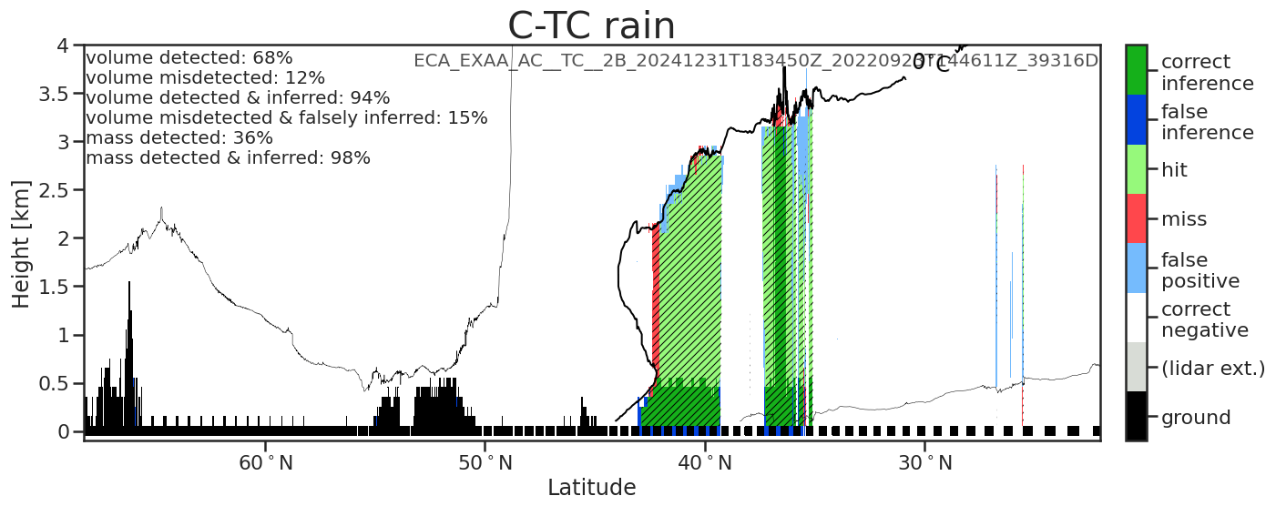
Figure 13An intercomparison of AC-TC detection of rain for the Halifax scene. The volume fraction is calculated from the fraction of pixels detected compared to those containing any rain in the GEM model after interpolation to the JSG (hatched areas). The mass fraction is based on the mass of rain from the GEM model. The total fractions in AC-TC include the inferred presence of rain that cannot be detected directly by the instrument but may be inferred, such as in regions of radar surface clutter contiguous with rain or where CPR is extinguished in deep convection. Atmospheric temperature contours from the model are overlaid. Grey shading indicates where each instrument is extinguished.
6.4 Aerosols
The detection of aerosols is made solely by ATLID, so we only evaluate A-TC here. The Halifax scene (Fig. 14) illustrates that some large areas of aerosols from the numerical model are not detected by A-TC; the target classification correctly identifies aerosols in around 38 % of pixels or around 43 % of aerosol mass content across the three test scenes. The aerosols that are undetected by the spaceborne lidar are either in low-concentration aerosol layers or are in parts of the atmosphere obscured by other hydrometeors. The aerosols that are below the sensitivity of the instrument include the elevated aerosol layer between 54 and 63 ∘ N in the Halifax scene, even when A-TC applies the longest horizontal integration scales, and at the edges of other layers. These missed aerosols represent around 30 % by volume across the three scenes and about 10 % of total aerosol mass content. The larger portion of missed aerosols is obscured by other targets; this represents around 32 % by volume and almost 50 % of the mass of aerosols across the three scenes.
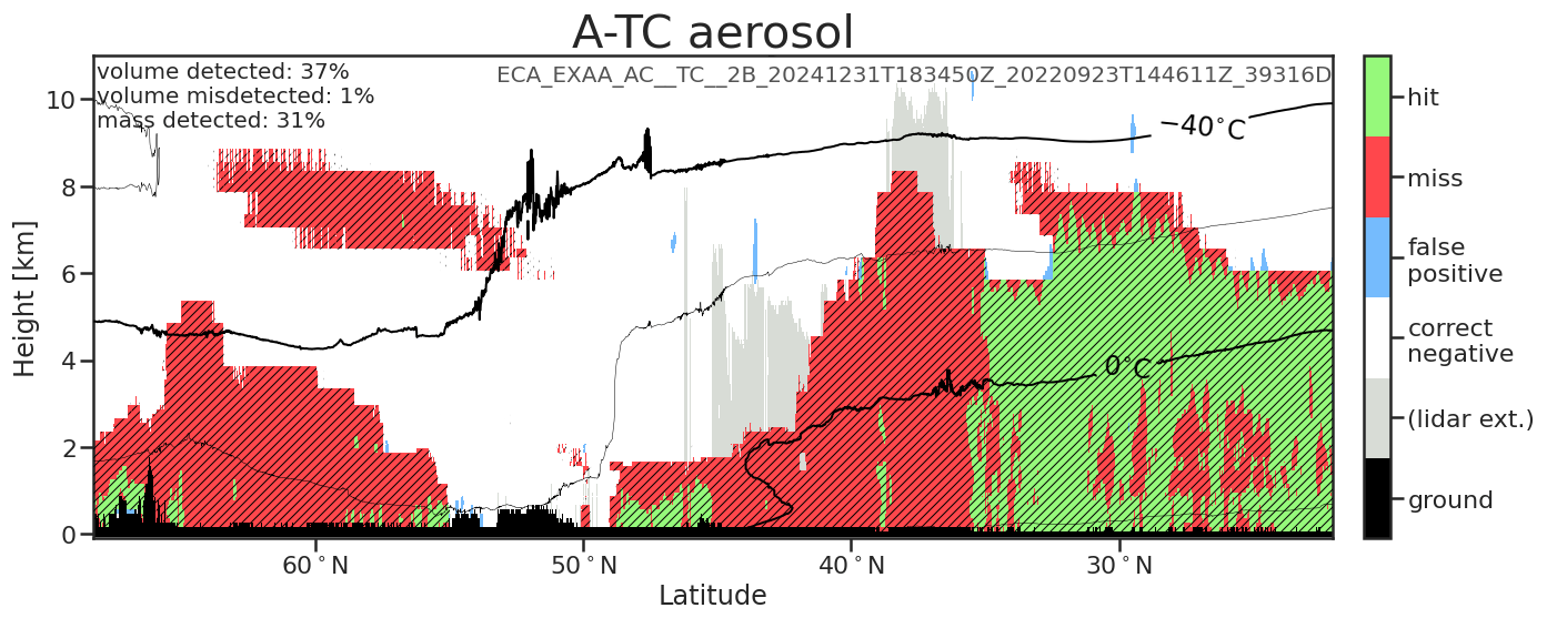
Figure 14An intercomparison of AC-TC detection of aerosol for the Halifax scene. The volume fraction is calculated from the fraction of pixels detected compared to those containing any aerosol in the GEM model after interpolation to the JSG (hatched areas). The mass fraction is based on the mass of aerosol from the GEM model. Atmospheric temperature contours from the model are overlaid.
False-positive identifications of aerosols are relatively rare but can be seen in the Halifax scene (Fig. 14) at the edges of ice clouds. Over the three test scenes, around 4 % of ice clouds by volume, representing a negligible fraction of total ice water content, are classified as aerosols, while around 6 % by volume and 7 % by mass of aerosols are classified as ice clouds.
The EarthCARE space mission is developed to probe the Earth's atmosphere, particularly for the measurement of profiles of clouds and aerosols which play an essential role in the balance of the Earth's radiative system. Its payload consists of a set of instruments to achieve these goals, including the high-spectral-resolution lidar ATLID and the CPR, a Doppler radar. A necessary condition for the retrieval of the physical properties of clouds, aerosols and precipitation from atmospheric profiles measured by each instrument is to accurately identify the presence of hydrometeors and aerosols. For this, a classification of atmospheric targets (hydrometeors and aerosols) has been established for each instrument, namely A-TC for ATLID target classification and C-TC for CPR target classification. The synergy between ATLID and CPR measurements can then be used to remove ambiguity in the target classifications. Indeed, ATLID is sensitive to the smallest particles (aerosols and cloud particles, even molecules), while the CPR is sensitive to the largest ones (large ice particles, snowflakes and raindrops). This is this same approach that was used in the analysis of the observations made with the lidar and the radar aboard CloudSat and CALIPSO, the two satellites of the A-Train constellation. It was this experience that led to the creation of the synergistic DARDAR-MASK products, which were leveraged by EarthCARE to create a similar product, AC-TC for ATLID CPR target classification. The novel capabilities of EarthCARE's active instruments are reflected in the single-instrument and synergistic target classifications; specifically, ATLID's measurement of lidar ratio is used to differentiate optically thin ice from aerosols and to accurately type different aerosol species (Sect. 2), while CPR's Doppler velocity measurements distinguish snow and rimed snow from ice cloud and provide vertically resolved information on the depth of the melting layer (Sect. 3).
How A-TC and C-TC classifications are derived from lidar and radar measurements was respectively described in Sects. 2 and 3. The Halifax scene, a numerical simulation of EarthCARE observations, is used to illustrate and test the different products created. The way the AC-TC classification is calculated from the A-TC and C-TC products, as well as the new radar–lidar synergy decision matrix created for EarthCARE, was detailed in Sect. 4. The tests and results obtained with the processors developed for the calculation of A-TC, C-TC and AC-TC were also presented. They showed that these products are correctly built when analysed with reference to the Halifax scene.
The production of simulated EarthCARE scenes has provided an opportunity for an omniscient evaluation by which we can quantify the detection efficiency of EarthCARE's active instruments and the benefits of their synergy (Sect. 6). The greatest area of radar–lidar synergy is in ice clouds, where A-TC and C-TC have areas of overlap (around 25 % of pixels containing ice clouds across the three test scenes) and complementary coverage with optically thin ice clouds seen only by ATLID (about 10 % by volume) and deep and precipitating ice seen only by CPR (about 30 % by volume).
The detection and classification of aerosols and liquid cloud are dominated by ATLID, and both are therefore strongly affected by the rapid extinction of the lidar; across the three test scenes, around 80 % of pixels containing liquid cloud were undetected due to extinction, while 30 % of pixels containing aerosols were obscured by extinction or by other targets (i.e. hydrometeors). The extinction of ATLID is communicated in AC-TC by the inclusion of possible-liquid classifications, which conveys the unknown presence of liquid cloud (or, indeed, aerosols) in parts of the atmosphere where only information from CPR is available. While C-TC includes liquid cloud classification, in practice, the radar signal is dominated by drizzle drops and snowflakes where present; hence, in parts of the profile where ATLID measurements are not available, the presence and physical depth of mixed-phase and liquid cloud layers remain difficult to diagnose. Indeed, across the three test scenes, less than 10 % of liquid cloud water was directly detected by ATLID. To better understand the extent of liquid clouds that are not apparent to ATLID, we have evaluated a simple set of assumptions that infer the presence of liquid cloud in areas co-located with the following three classifications made by CPR: all rain classes, rimed snow when ATLID is extinguished and the heavy precipitation classifications made when CPR is overwhelmed by multiple scattering and attenuation. Evaluation over the three test scenes showed that the coarse assumption allowed a majority of liquid cloud water content to be accounted for, specifically around 75 % of liquid water content, which is up from around 10 % directly detected by the active instruments. This evaluation using clouds from a numerical weather model shows a significant underestimation of liquid clouds by spaceborne radar–lidar synergy that has long been acknowledged, but difficult to quantify, in CloudSat-CALIPSO target classifications. Indeed, liquid cloud within rain is already assumed within CloudSat rain retrievals (Lebsock and L'Ecuyer, 2011). A simplified retrieval of liquid cloud based on these inferences is made in EarthCARE's synergistic retrieval algorithm (ACM-CAP) and is evaluated in Mason et al. (2022).
The classification of precipitation is solely informed by CPR; C-TC accurately identifies around two-thirds of all rainy pixels, representing around one-third of rain water content, across the three test scenes. Two limits on the detection of rain by CPR are radar ground clutter within around 500 m of the surface and when the radar signal is overcome by multiple scattering and attenuation in heavy precipitation. When cautious assumptions are made to infer the presence of rain in these situations – assuming rain is continuous to the surface through clutter when contiguous with rain detected above the surface clutter and in convective cores – more than 95 % of rain water content can be accounted for. Similar inferences can also be used to improve the detection of snow in C-TC and AC-TC; across the three test scenes, more than 30 % of ice water content was within deep convective cores or the surface clutter zone. All such inferred precipitation classes are distinguished within the C-TC and AC-TC products from those based directly on measurements; their inclusion is intended to prevent biases in the spatial distribution of precipitation provided by the target classification products, and they are used within the synergistic retrieval algorithm ACM-CAP to permit continuous (if more uncertain) retrievals of cloud and precipitation through heavy-precipitation features (Mason et al., 2022).
EarthCARE's target classification products build upon the success of DARDAR-MASK products from CloudSat-CALIPSO. The following three target classification algorithms and L2 data products have been introduced: A-TC for ATLID, C-TC for CPR and the synergistic product AC-TC. AC-TC will provide continuity with DARDAR-MASK while taking advantage of EarthCARE's novel capabilities, namely an improved detection of rimed snow from CPR's Doppler velocity and a probabilistic aerosol discrimination framework using ATLID's measurements of depolarisation and lidar ratio.
The EarthCARE Level-2 demonstration products from simulated scenes, including the A-TC, C-TC and AC-TC products discussed in this paper, are available from https://doi.org/10.5281/zenodo.7728948 (van Zadelhoff et al., 2023a).
All the authors of this paper, namely AI, JD, GJvZ, DD, PK, AT, SM, RJH and BPT contributed fairly with regard to the development of the studies that led to the results presented here. They also contributed equally to the writing and correction of the different parts of the paper for which they are responsible.
The contact author has declared that none of the authors has any competing interests.
Publisher’s note: Copernicus Publications remains neutral with regard to jurisdictional claims in published maps and institutional affiliations.
This article is part of the special issue “EarthCARE Level 2 algorithms and data products”. It is not associated with a conference.
This research has been supported by the European Space Agency (grant nos. 4000112030/15/NL/CT (DORSY) and 4000134661/21/NL/AD (CARDINAL)).
This paper was edited by Hajime Okamoto and reviewed by two anonymous referees.
Barker, H. W., Cole, J. N. S., Qu, Z., Villefranque, N., and Shephard, M.: Radiative closure assessment of retrieved cloud and aerosol properties for the EarthCARE mission: the ACMB-DF product, Atmos. Meas. Tech., in preparation, 2023. a
Battaglia, A., Augustynek, T., Tanelli, S., and Kollias, P.: Multiple scattering identification in spaceborne W-band radar measurements of deep convective cores, J. Geophys. Res., 116, D19201, https://doi.org/10.1029/2011JD016142, 2011. a
Burns, D., Kollias, P., Tatarevic, A., Battaglia, A., and Tanelli, S.: The performance of the EarthCARE Cloud Profiling Radar in marine stratiform clouds, J. Geophys. Res.-Atmos., 121, 14525–14537, https://doi.org/10.1002/2016JD025090, 2016. a
Ceccaldi, M., Delanoë, J., Hogan, R. J., Pounder, N. L., Protat, A., and Pelon, J.: From CloudSat-CALIPSO to EarthCare: Evolution of the DARDAR cloud classification and its comparison to airborne radar-lidar observations, J. Geophys. Res.-Atmos., 118, 7962–7981, https://doi.org/10.1002/jgrd.50579, 2013. a, b, c, d
Chandra, A. S., Kollias, P., and Albrecht, B. A.: Multiyear Summertime Observations of Daytime Fair-Weather Cumuli at the ARM Southern Great Plains Facility, J. Climate, 26, 10031–10050, https://doi.org/10.1175/JCLI-D-12-00223.1, 2013. a
Delanoë, J. and Hogan, R. J.: Combined CloudSat-CALIPSO-MODIS retrievals of the properties of ice clouds, J. Geophys. Res.-Atmos., 115, D00H29, https://doi.org/10.1029/2009JD012346, 2010. a, b, c
do Carmo, J. P., de Villele, G., Wallace, K., Lefebvre, A., Ghose, K., Kanitz, T., Chassat, F., Corselle, B., Belhadj, T., and Bravetti, P.: ATmospheric LIDar (ATLID): Pre-Launch Testing and Calibration of the European Space Agency Instrument That Will Measure Aerosols and Thin Clouds in the Atmosphere, Atmosphere, 12, 76, https://doi.org/10.3390/atmos12010076, 2021. a
Donovan, D. P., Klein Baltink, H., Henzing, J. S., de Roode, S. R., and Siebesma, A. P.: A depolarisation lidar-based method for the determination of liquid-cloud microphysical properties, Atmos. Meas. Tech., 8, 237–266, https://doi.org/10.5194/amt-8-237-2015, 2015. a
Donovan, D. P., Kollias, P., Velázquez Blázquez, A., and van Zadelhoff, G.-J.: The Generation of EarthCARE L1 Test Data sets Using Atmospheric Model Data Sets, EGUsphere [preprint], https://doi.org/10.5194/egusphere-2023-384, 2023a. a, b, c, d, e
Donovan, D. P., van Zadelhoff, G.-J., and Wang, P.: The EarthCARE lidar cloud and aerosol profile processor: the A-AER, A-EBD, A-TC and A-ICE products, Atmos. Meas. Tech., in preparation, 2023b. a, b, c, d, e
Eisinger, M., Wehr, T., Kubota, T., Bernaerts, D., Wallace, K., and Marnas, F.: The EarthCARE Mission – Science Data Processing Chain Overview, Atmos. Meas. Tech., in preparation, 2023b. a, b, c, d, e
Fox, N. I. and Illingworth, A. J.: The Retrieval of Stratocumulus Cloud Properties by Ground-Based Cloud Radar, J. Appl. Meteorol., 36, 485–492, https://doi.org/10.1175/1520-0450(1997)036<0485:TROSCP>2.0.CO;2, 1997. a
Frisch, A. S., Fairall, C. W., and Snider, J. B.: Measurement of Stratus Cloud and Drizzle Parameters in ASTEX with a Kα-Band Doppler Radar and a Microwave Radiometer, J. Atmos. Sci., 52, 2788–2799, https://doi.org/10.1175/1520-0469(1995)052<2788:MOSCAD>2.0.CO;2, 1995. a
Geerts, B. and Dawei, Y.: Classification and Characterization of Tropical Precipitation Based on High-Resolution Airborne Vertical Incidence Radar. Part I: Classification, J. Appl. Meteorol., 43, 1554–1566, 2004. a
Hu, Y., Vaughan, M., Liu, Z., Lin, B., Yang, P., Flittner, D., Hunt, B., Kuehn, R., Huang, J., Wu, D., Rodier, S., Powell, K., Trepte, C., and Winker, D.: The depolarization–attenuated backscatter relation: CALIPSO lidar measurements vs. theory, Opt. Express, 15, 5327–5332, 2007. a
Hu, Y., Winker, D., Vaughan, M., Lin, B., Omar, A., Trepte, C., Flittner, D., Yang, P., Nasiri, S. L., Baum, B., Holz, R., Sun, W., Liu, Z., Wang, Z., Young, S., Stamnes, K., Huang, J., and Kuehn, R.: CALIPSO/CALIOP Cloud Phase Discrimination Algorithm, J. Atmos. Ocean. Tech., 26, 2293–2309, https://doi.org/10.1175/2009JTECHA1280.1, 2009. a
Huang, Y., Siems, S. T., Manton, M. J., Protat, A., and Delanoë, J.: A study on the low-altitude clouds over the Southern Ocean using the DARDAR-MASK, J. Geophys. Res.-Atmos., 117, D18204, https://doi.org/10.1029/2012JD017800, 2012. a
Illingworth, A. J., Hogan, R. J., O'Connor, E. J., Bouniol, D., Delanoë, J., Pelon, J., Protat, A., Brooks, M. E., Gaussiat, N., Wilson, D. R., Donovan, D. P., Baltink, H. K., van Zadelhoff, G.-J., Eastment, J. D., Goddard, J. W. F., Wrench, C. L., Haeffelin, M., Krasnov, O. A., Russchenberg, H. W. J., Piriou, J.-M., Vinit, F., Seifert, A., Tompkins, A. M., and Willén, U.: Cloudnet, B. Am. Meteorol. Soc., 88, 883–898, https://doi.org/10.1175/BAMS-88-6-883, 2007. a, b
Illingworth, A. J., Barker, H. W., Beljaars, A., Ceccaldi, M., Chepfer, H., Clerbaux, N., Cole, J., Delanoë, J., Domenech, C., Donovan, D. P., Fukuda, S., Hirakata, M., Hogan, R. J., Huenerbein, A., Kollias, P., Kubota, T., Nakajima, T., Nakajima, T. Y., Nishizawa, T., Ohno, Y., Okamoto, H., Oki, R., Sato, K., Satoh, M., Shephard, M. W., Velázquez-Blázquez, A., Wandinger, U., Wehr, T., and van Zadelhoff, G.-J.: The EarthCARE Satellite: The Next Step Forward in Global Measurements of Clouds, Aerosols, Precipitation, and Radiation, B. Am. Meteorol. Soc., 96, 1311–1332, https://doi.org/10.1175/BAMS-D-12-00227.1, 2015. a, b, c
Kollias, P., Miller, M. A., Johnson, K. L., Jensen, M. P., and Troyan, D. T.: Cloud, thermodynamic, and precipitation observations in West Africa during 2006, J. Geophys. Res.-Atmos., 114, D00E08, https://doi.org/10.1029/2008JD010641, 2009. a
Kollias, P., Rémillard, J., Luke, E., and Szyrmer, W.: Cloud radar Doppler spectra in drizzling stratiform clouds: 1. Forward modeling and remote sensing applications, J. Geophys. Res.-Atmos., 116, D13201, https://doi.org/10.1029/2010JD015237, 2011. a
Kollias, P., Jo, I., Borque, P., Tatarevic, A., Lamer, K., Bharadwaj, N., Widener, K., Johnson, K., and Clothiaux, E. E.: Scanning ARM Cloud Radars. Part II: Data Quality Control and Processing, J. Atmos. Ocean. Tech., 31, 583–598, https://doi.org/10.1175/JTECH-D-13-00045.1, 2014. a
Kollias, P., Puidgomènech Treserras, B., Battaglia, A., Borque, P., and Tatarevic, A.: Processing reflectivity and Doppler velocity from EarthCARE’s cloud profiling radar: the C-FMR, C-CD and C-APC products, EGUsphere [preprint], https://doi.org/10.5194/egusphere-2022-1284, 2022. a, b
Krasnov, O. and Russchenberg, H.: A synergetic radar-lidar technique for the LWC retrieval in water clouds description and application to cloudnet data, in: The 11th Conference on Mesoscale Processes and the 32nd Conference on Radar Meteorology, Albuquerque, New Mexico, 23–29 October 2005, American Meteorology Society, 1–13, 2005. a
Lamer, K. and Kollias, P.: Observations of fair-weather cumuli over land: Dynamical factors controlling cloud size and cover, Geophys. Res. Lett., 42, 8693–8701, https://doi.org/10.1002/2015GL064534, 2015. a
Lebsock, M. D. and L'Ecuyer, T. S.: The retrieval of warm rain from CloudSat, J. Geophys. Res., 116, D20209, https://doi.org/10.1029/2011JD016076, 2011. a
Listowski, C., Delanoë, J., Kirchgaessner, A., Lachlan-Cope, T., and King, J.: Antarctic clouds, supercooled liquid water and mixed phase, investigated with DARDAR: geographical and seasonal variations, Atmos. Chem. Phys., 19, 6771–6808, https://doi.org/10.5194/acp-19-6771-2019, 2019. a, b
Listowski, C., Rojo, M., Claud, C., Delanoë, J., Rysman, J.-F., Cazenave, Q., and Noer, G.: New Insights Into the Vertical Structure of Clouds in Polar Lows, Using Radar-Lidar Satellite Observations, Geophys. Res. Lett., 47, e2020GL088785, https://doi.org/10.1029/2020GL088785, 2020. a, b
Liu, Y., Geerts, B., Miller, M., Daum, P., and McGraw, R.: Threshold radar reflectivity for drizzling clouds, Geophys. Res. Lett., 35, L03807, https://doi.org/10.1029/2007GL031201, 2008. a
Luke, E. P., Kollias, P., Johnson, K. L., and Clothiaux, E. E.: A Technique for the Automatic Detection of Insect Clutter in Cloud Radar Returns, J. Atmos. Ocean. Tech., 25, 1498–1513, https://doi.org/10.1175/2007JTECHA953.1, 2008. a
Mace, G. G. and Sassen, K.: A constrained algorithm for retrieval of stratocumulus cloud properties using solar radiation, microwave radiometer, and millimeter cloud radar data, J. Geophys. Res.-Atmos., 105, 29099–29108, https://doi.org/10.1029/2000JD900403, 2000. a, b
Mace, G. G. and Zhang, Q.: The CloudSat radar-lidar geometrical profile product (RL-GeoProf): Updates, improvements, and selected results, J. Geophys. Res.-Atmos., 119, 9441–9462, https://doi.org/10.1002/2013JD021374, 2014. a
Marchand, R., Mace, G. G., Ackerman, T., and Stephens, G.: Hydrometeor Detection Using Cloudsat—An Earth-Orbiting 94-GHz Cloud Radar, J. Atmos. Ocean. Tech., 25, 519–533, https://doi.org/10.1175/2007JTECHA1006.1, 2008. a
Mason, S., Jakob, C., Protat, A., and Delanoë, J.: Characterizing Observed Midtopped Cloud Regimes Associated with Southern Ocean Shortwave Radiation Biases, J. Climate, 27, 6189–6203, https://doi.org/10.1175/JCLI-D-14-00139.1, 2014. a
Mason, S. L., Hogan, R. J., Bozzo, A., and Pounder, N. L.: A unified synergistic retrieval of clouds, aerosols and precipitation from EarthCARE: the ACM-CAP product, EGUsphere [preprint], https://doi.org/10.5194/egusphere-2022-1195, 2022. a, b, c, d, e, f, g
Mioche, G., Jourdan, O., Ceccaldi, M., and Delanoë, J.: Variability of mixed-phase clouds in the Arctic with a focus on the Svalbard region: a study based on spaceborne active remote sensing, Atmos. Chem. Phys., 15, 2445–2461, https://doi.org/10.5194/acp-15-2445-2015, 2015. a, b
Mioche, G., Jourdan, O., Delanoë, J., Gourbeyre, C., Febvre, G., Dupuy, R., Monier, M., Szczap, F., Schwarzenboeck, A., and Gayet, J.-F.: Vertical distribution of microphysical properties of Arctic springtime low-level mixed-phase clouds over the Greenland and Norwegian seas, Atmos. Chem. Phys., 17, 12845–12869, https://doi.org/10.5194/acp-17-12845-2017, 2017. a, b
Mülmenstädt, J., Sourdeval, O., Delanoë, J., and Quaas, J.: Frequency of occurrence of rain from liquid-, mixed-, and ice-phase clouds derived from A-Train satellite retrievals, Geophys. Res. Lett., 42, 6502–6509, https://doi.org/10.1002/2015GL064604, 2015. a
Qu, Z., Donovan, D. P., Barker, H. W., Cole, J. N. S., Shephard, M. W., and Huijnen, V.: Numerical Model Generation of Test Frames for Pre-launch Studies of EarthCARE's Retrieval Algorithms and Data Management System, Atmos. Meas. Tech. Discuss. [preprint], https://doi.org/10.5194/amt-2022-300, in review, 2022. a, b, c, d
Stephens, G., Winker, D., Pelon, J., Trepte, C., Vane, D., Yuhas, C., L’Ecuyer, T., and Lebsock, M.: CloudSat and CALIPSO within the A-Train: Ten Years of Actively Observing the Earth System, B. Am. Meteorol. Soc., 99, 569–581, https://doi.org/10.1175/BAMS-D-16-0324.1, 2018. a
Stephens, G. G. L., Vane, D. D. G., Tanelli, S., Im, E., Durden, S., Rokey, M., Reinke, D., Partain, P., Mace, G. G., Austin, R., L'Ecuyer, T., Haynes, J., Lebsock, M., Suzuki, K., Waliser, D., Wu, D., Kay, J., Gettelman, A., Wang, Z., and Marchand, R.: CloudSat mission: Performance and early science after the first year of operation, J. Geophys. Res., 113, D00A18, https://doi.org/10.1029/2008JD009982, 2008. a
van Zadelhoff, G.-J., Barker, H. W., Baudrez, E., Bley, S., Clerbaux, N., Cole, J. N. S., de Kloe, J., Docter, N., Domenech, C., Donovan, D. P., Dufresne, J.-L., Eisinger, M., Fischer, J., García-Marañón, R., Haarig, M., Hogan, R. J., Hünerbein, A., Kollias, P., Koopman, R., Madenach, N., Mason, S. L., Preusker, R., Puigdomènech Treserras, B., Qu, Z., Ruiz-Saldaña, M., Shephard, M., Velázquez-Blazquez, A., Villefranque, N., Wandinger, U., Wang, P., and Wehr, T.: EarthCARE level-2 demonstration products from simulated scenes, Version 10.10, Zenodo [data set], https://doi.org/10.5281/zenodo.7728948, 2023a. a
van Zadelhoff, G.-J., Donovan, D. P., and Wang, P.: Detection of aerosol and cloud features for the EarthCARE lidar ATLID: the A-FM product, EGUsphere [preprint], https://doi.org/10.5194/egusphere-2023-145, 2023b. a, b
Vérèmes, H., Listowski, C., Delanoë, J., Barthe, C., Tulet, P., Bonnardot, F., and Roy, D.: Spatial and seasonal variability of clouds over the southwest Indian Ocean based on the DARDAR mask product, Q. J. Roy. Meteor. Soc., 145, 3561–3576, https://doi.org/10.1002/qj.3640, 2019. a, b
Wandinger, U., Floutsi, A. A., Baars, H., Haarig, M., Ansmann, A., Hünerbein, A., Docter, N., Donovan, D., van Zadelhoff, G.-J., Mason, S., and Cole, J.: HETEAC – the Hybrid End-To-End Aerosol Classification model for EarthCARE, Atmos. Meas. Tech., 16, 2485–2510, https://doi.org/10.5194/amt-16-2485-2023, 2023. a
Wehr, T., Kubota, T., Tzeremes, G., Wallace, K., Nakatsuka, H., Ohno, Y., Koopman, R., Rusli, S., Kikuchi, M., Eisinger, M., Tanaka, T., Taga, M., Deghaye, P., Tomita, E., and Bernaerts, D.: The EarthCARE Mission – Science and System Overview, EGUsphere [preprint], https://doi.org/10.5194/egusphere-2022-1476, 2023. a, b, c
Winker, D. M., Pelon, J., Coakley, J. A., Ackerman, S. A., Charlson, R. J., Colarco, P. R., Flamant, P., Fu, Q., Hoff, R. M., Kittaka, C., Kubar, T. L., Le Treut, H., Mccormick, M. P., Mégie, G., Poole, L., Powell, K., Trepte, C., Vaughan, M. A., and Wielicki, B. A.: The CALIPSO Mission, B. Am. Meteorol. Soc., 91, 1211–1230, https://doi.org/10.1175/2010BAMS3009.1, 2010. a
Zhu, Z., Kollias, P., Luke, E., and Yang, F.: New insights on the prevalence of drizzle in marine stratocumulus clouds based on a machine learning algorithm applied to radar Doppler spectra, Atmos. Chem. Phys., 22, 7405–7416, https://doi.org/10.5194/acp-22-7405-2022, 2022. a
- Abstract
- Introduction
- ATLID target classification: A-TC
- CPR target classification: C-TC
- The synergistic target classification: AC-TC
- Case study: tests with the Halifax scene
- Evaluation
- Conclusion
- Data availability
- Author contributions
- Competing interests
- Disclaimer
- Special issue statement
- Financial support
- Review statement
- References