the Creative Commons Attribution 4.0 License.
the Creative Commons Attribution 4.0 License.
 | 09 Jun 2023
Cloud and precipitation microphysical retrievals from the EarthCARE Cloud Profiling Radar: the C-CLD product
Bernat Puidgomènech Treserras
Alessandro Battaglia
Pavlos Kollias
Aleksandra Tatarevic
Frederic Tridon
The Earth Clouds, Aerosols and Radiation Explorer (EarthCARE) satellite mission is a joint endeavour developed by the European Space Agency (ESA) and the Japan Aerospace Exploration Agency (JAXA) and features a 94 GHz Doppler Cloud Profiling Radar. This paper presents the theoretical basis of the cloud and precipitation microphysics (C-CLD) EarthCARE Level 2 (L2) algorithm. The C-CLD algorithm provides the best estimates of the vertical profiles of water mass content and hydrometeor characteristic size, obtained from radar reflectivity, path-integrated signal attenuation and hydrometeor sedimentation Doppler velocity estimates using optimal estimation (OE) theory. To obtain the forward model relations and the associated uncertainty, an ensemble-based method is used. This ensemble consists of a collection of in situ measured drop size distributions that cover natural microphysical variability. The ensemble mean and standard deviation represent the forward model relations and their microphysics-based uncertainty. The output variables are provided on the joint standard grid horizontal and EarthCARE Level 1b (L1b) vertical grid (1 km along track and 100 m vertically). The OE framework is not applied to liquid-only clouds in drizzle-free and lightly drizzling conditions, where a more statistical approach is preferred.
- Article
(6421 KB) - Full-text XML
- BibTeX
- EndNote


Clouds and precipitation systems play a critical role in Earth's energy and hydrological cycle (Stephens et al., 2010, 2012). The accurate representation of cloud and precipitation systems in numerical models is essential for improving the predictability of weather and climate models. While surface-based observatories (Illingworth et al., 2007; Mather and Voyles, 2013; Kollias et al., 2020) can provide high-resolution observations suitable for process studies, satellite-based active remote sensors have the potential to obtain global estimates of cloud and precipitation microphysics and dynamics (Battaglia et al., 2020b). The National Aeronautics and Space Administration (NASA) A-Train satellite constellation (Stephens et al., 2002, 2018) first demonstrated the potential of active remote sensing from space. The Earth Clouds, Aerosols and Radiation Explorer (EarthCARE) mission (Wehr et al., 2023) scheduled for launch in 2024 features the first spaceborne Cloud Profiling Radar (CPR) with Doppler capability (Illingworth et al., 2015; Kollias et al., 2022a, b). The EarthCARE CPR observations will offer a unique opportunity for the collection of a global dataset of vertical motions and microphysics in clouds and precipitation.
Compared to CloudSat, the EarthCARE CPR has higher sensitivity (5–6 dB more sensitive), better vertical sampling (100 versus 240 m), higher along-track resolution (500 versus 1100 m) and a smaller instantaneous field of view (IFOV, 800 versus 1400 m) and includes Doppler velocity measurements and improved detection in the lowest atmosphere levels (Illingworth et al., 2015; Battaglia et al., 2020b; Burns et al., 2016; Lamer et al., 2019; Kollias et al., 2014). Based on these characteristics, the EarthCARE CPR is expected to provide an improved set of CPR observables, i.e. radar reflectivity, path-integrated attenuation (PIA) and Doppler velocity, which after their post-processing and quality control by the CPR processor (C-PRO) algorithms (Kollias et al., 2022b) will be used for the development of the CPR-only cloud and precipitation microphysics (C-CLD) product.
The long record of CloudSat observations and the parallel development and validation of the CloudSat data products provide a strong heritage for the C-CLD algorithm development. In particular, the use of the CloudSat CPR path-integrated attenuation (PIA in dB) for estimating the total liquid water path (LWP) in the atmospheric column and for constraining surface and profile estimates of the rainfall rate (Haynes et al., 2009; Lebsock and L'Ecuyer, 2011) is applied in a similar manner in C-CLD. Another factor that influenced the C-CLD algorithm development is the development of sophisticated ground-based networks such as the U.S. Department of Energy Atmospheric Radiation Measurement (ARM) observatories and the pan-European Aerosol, Clouds and Trace Gases Research Infrastructure (ACTRIS) (Illingworth et al., 2007; Mather and Voyles, 2013; Kollias et al., 2020). The measurements from these surface-based networks have stimulated the development of several algorithms that utilize the combination of radar reflectivity and mean Doppler velocity (Delanoë et al., 2007; Heymsfield et al., 2008; Mason et al., 2018; Oue et al., 2019). These efforts highlighted the information content of the Doppler velocity that is a new EarthCARE CPR observable from space compared to CloudSat. In addition, the C-CLD algorithm utilizes our latest understanding of solid hydrometeors scattering at 94 GHz (Hogan and Westbrook, 2014; Kneifel et al., 2020) and the availability of extensive ground-based observations of particle size distributions (Williams, 2012; von Lerber et al., 2017).
The C-CLD cloud and precipitation retrieval algorithm is based on a profile-by-profile approach. At each profile, it uses information available from the radar-only measurements provided in the form of the following products, as described by Kollias et al. (2022b): the CPR feature mask and radar reflectivity (C-FMR), CPR cloud Doppler (C-CD) parameters, and CPR target classification (C-TC). The C-CLD algorithm derives the best estimates of cloud and precipitation microphysics that feed into the composite cloud and aerosol profiles product (ACM-COM, ATmospheric LIDar–Cloud Profiling Radar–MultiSpectral Instrument composite; Cole et al., 2022) as explained in Eisinger et al. (2023). The main retrieved quantities consist of the water mass content and particle characteristic size. First, the output of the C-TC hydrometeor classification is used to determine the occurrence of the specific hydrometeor type (ice cloud, snow, rimed snow, melting snow, cold rain, warm rain, non-drizzling liquid cloud, drizzling liquid cloud). This information is used to determine which branch of the C-CLD retrieval will be employed.
As illustrated in the flowchart shown in Fig. 1, the C-CLD processor contains specific algorithms designed to retrieve distinct cloud system types:
- a.
liquid cloud retrieval with the separation between non-drizzling and drizzling liquid clouds;
- b.
ice cloud retrieval and precipitation retrieval with specific algorithms designed to retrieve ice cloud, snow, riming snow, cold rain and warm rain.
The optimal estimation (OE) variational approach is applied as described in Rodgers (2000). It is based on a Gauss–Newton minimization algorithm that allows for a quantitative evaluation of the uncertainty in the retrieved quantities. The forward model within the OE approach maps two moments of the particle size distribution (PSD), the particle characteristic size (Dm; i.e. mean-mass-weighted equivalent melted diameter) and mass water content (MC) to the CPR reflectivity and Doppler velocity (previously corrected in C-CD for vertical air motion).
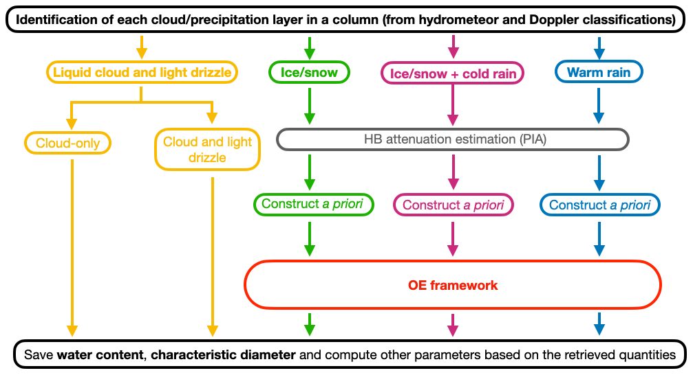
Figure 1Cloud and precipitation retrieval scheme flow chart. OE theory is applied in the retrieval of solid and liquid precipitating clouds. The retrievals in the liquid clouds and lightly drizzling clouds (yellow box) are not performed using the OE method. HB: Hitschfeld and Bordan (1954).
The OE method is not applied for retrieval of drizzle-free clouds (i.e. non-precipitating liquid clouds) and for lightly drizzling clouds (group a). This is justified by the following facts.
-
In the case of drizzle-free clouds, observed Doppler velocity does not provide any relevant information (fall velocity of the cloud droplet is negligible), so the reflectivity is the only measurement available.
-
In the case of lightly drizzling clouds, the observed Doppler velocity could be heavily dominated by vertical air motion, leading to a large uncertainty in the reflectivity-weighted velocity. Moreover, the observed reflectivity is, in general, dominated by drizzle.
Therefore, a retrieval approach involving the optimal estimation method and much simpler methods based on the use of power-law relationships will result in similar uncertainties in microphysical parameters. The main retrieved variables for liquid clouds and drizzle are liquid water content and particle effective diameter, i.e. the ratio of the third and the second PSD moments. Note that the case of heavy drizzle is included in the rain retrieval, as a subcategory of warm rain.
The individual algorithms will now be described in detail in the next sections.
2.1 Liquid cloud and light-drizzle retrieval
Two distinct situations are analysed: non-precipitating liquid clouds and clouds that generate light drizzle. These two scenarios do not overlap spatially with each other or with pixels classified as precipitation, where the OE algorithm is used. When a radar volume is classified as a liquid cloud or light drizzle, an appropriate power-law formula is utilized to estimate the combined liquid water content of the cloud and any drizzle that may be present. In the case of the OE retrieval, the liquid water path is one of the retrieved state vector unknowns. Once retrieved, it is distributed adiabatically in the column to provide an estimate of the liquid water content. The algorithm clearly distinguishes between the cloud water and the precipitation mass content, with the latter being equal to 0 for liquid clouds and light drizzle.
2.1.1 Drizzle-free clouds
The cloud liquid water content (LWC) vertical structure is determined from the reflectivity values using the relationship LWC−Ze, derived in a power-law form:
where 〈A〉 is an average value assumed constant across the whole height (Frisch et al., 1998). This relationship assumes that both the cloud droplets' number concentration and the PSD spectral width are constant with height. While this is reasonable in marine clouds (e.g. Miles et al., 2000), Löhnert and Crewell (2003) concluded that this assumption is the dominant error factor in continental clouds. If a measurable PIA signal is available, we can estimate the liquid water path (LWP) and subsequently estimate the parameter 〈A〉. Otherwise, two constant values of 4.7 and 2.4 g mm−3 m are assumed over land and ocean, for 〈A〉, respectively.
The corresponding cloud LWP obtained from such an approximation is evaluated against the estimated cloud mass content adiabatic profile that represents an average in-cloud profile, independent of the reflectivity vertical variability with LWC increasing with the distance from the cloud base, as
where the term in the square brackets accounts for a decrease in adiabaticity in the thicker clouds as proposed in Wood et al. (2009), z0w is a scaling parameter set to 500 m, Γw is the average vertical gradient of the change in adiabatic LWC (parameterized in Eq. B1), hcb is the height of the cloud base and fwN is a normalization factor that is set to 1. In the case of unreliable LWP estimates (i.e. when there is more than one cloud layer and the PIA corresponding to the cloud is smaller than 2 dB), a minimum and a maximum limit of the adiabatic profile (0.3LWCad and 0.9LWCad, respectively) is enforced on the estimate from the power-law formula.
The cloud effective radius is computed as a mean between the relationship proposed by Fox and Illingworth (1997),
and a relation derived for a lognormal PSD with a spectra width of 0.38 µm reported by Miles et al. (2000) as an average value,
In Eqs. (3) and (4), reff is in micrometres; Z is in mm6 m−3; and the number concentration Ncl is per cubic centimetres and is assumed to be equal to 288 and 74 over land and ocean, respectively (Miles et al., 2000).
2.1.2 Lightly drizzling clouds
The retrieval of LWC for lightly drizzling clouds combines two estimates:
-
the LWC derived from reflectivity based on power laws derived by Sauvageot and Omar (1987) and Baedi et al. (2000),
and a linear interpolation between these two for the intermediary reflectivity regime (−22 to −15 dBZ);
-
the LWC profile derived from the adiabatic model (Eq. 2) with fwN set to fit LWP estimates, if present, or otherwise set to 1.
The final LWCs are computed by combining the LWCad derived from the adiabatic model and LWCZ from the reflectivity profile. The used LWC–Z relation for drizzling conditions represents an average relation and can introduce a large bias, mainly close to the cloud base and cloud top; in such regions, large differences between LWCad and LWCZ are expected. Therefore, in the calculation of the LWC the weight attached to LWCZ is progressively reduced where the absolute relative difference between LWCad and LWCZ becomes large.
Note that the estimate of the liquid water content reported here includes both cloud and drizzle water content.
2.2 Optimal estimation framework components
For solid/liquid precipitation and ice clouds, the C-CLD algorithm applies a variational approach (Rodgers, 2000). It assimilates radar measurements and aims at balancing these data with the prior information to provide an optimal estimate of the state vector. Gauss–Newton iterations are used to find the best solution, which allows for a quantitative evaluation of the uncertainty in the retrieved quantities. This approach has been applied to similar radar-based microphysical retrievals in the past years (Lebsock and L'Ecuyer, 2011; Szyrmer et al., 2012; Battaglia et al., 2016, 2020c; Tridon et al., 2019a; Mason et al., 2017) and in the EarthCARE synergistic microphysical retrieval product (ACM-CAP, ATmospheric LIDar–Cloud Profiling Radar–MultiSpectral Instrument CAPTIVATE; Mason et al., 2022).
Radar measurements depend on a number of microphysical properties of hydrometeors in the sampled volume, including the particle size distribution (PSD) and, for solid-phase particles, the shape and mass distribution. Assumptions on any of the parameters listed above lead to a variety of microphysical relations reported in the literature between radar observables and microphysical properties (e.g. Protat et al., 2007; Matrosov and Turner, 2018). To assess the effect of the uncertainty associated with the microphysical description, the ensemble-based method is used to obtain the forward model relations and the associated simulation uncertainty. The ensemble consists of a number of particle size distributions collected at the ground for the Global Precipitation Measurement (GPM) mission ground validation programme (Dolan et al., 2018). Scattering models are applied to these data to map the microphysical quantities to the radar observables. The ensemble mean relations and its spread, defined as 1 standard deviation, represent the forward model relations and their microphysics associated uncertainty, respectively.
2.2.1 State vector
The PSD is parameterized using the concept of double-moment normalization. Following Delanoë et al. (2005), the normalizing moments are defined as
where p is the moment, D is the equivalent liquid sphere diameter and Dmax is the diameter of the largest particle. The ratio of the fourth and the third moment represents the mean-mass-weighted melted diameter and is used as the size scaling parameter, while M3 is proportional to the water-equivalent mass content that controls the magnitude of the PSD. Dmax is set to be equal to 5 mm or 2.5Dm, whichever value is smaller. By selecting M3 and M4 moments, the PSD can be expressed as
where f represents functional forms that are reported in the literature, derived from large datasets for each given hydrometeor category.
The goal of the C-CLD algorithm is to retrieve two moments of the PSD, i.e. the mass content, MC, and Dm, from radar reflectivity and Doppler velocity measurements. Therefore, the vector of the retrieval unknowns has the following form:
where N is the total number of the CPR range gates, regardless of whether they include ice/snow or rain. It is important to note that we do not use a separate notation for the mass content of ice and rain in this study, although it is commonly referred to as “ice water content” (IWC) and “rain water content” (RWC) in the literature. In case of warm- and cold-rain retrieval, the vector x also includes the cloud liquid water path with liquid water content distributed according to Eq. (2). In cold rain, the attenuation of the melting layer is an additional unknown. Note that the errors in the variables in the logarithmic units can be converted to fractional errors in the variable in the linear scale by the following error propagation formula:
where z=10x and x is either log 10Dm or log 10MC, e.g. the root mean square error in log 10z of 0.3 corresponds to the fractional error of 69 % in z.
2.2.2 Vector of measurements
The forward model maps the retrieved microphysical parameters to the space of radar measurements (attenuated radar reflectivity Zm; Doppler velocity corrected for air motion UD; and, in some cases, path-integrated attenuation).
The equivalent reflectivity factor for a radar operating at the wavelength λ is given by
where σb is the backscattering cross-section of a particle and Kw is the dielectric factor of liquid water at a reference temperature and frequency. For this study, Kw is assumed to be equal to 3.195+1.667i, which represents its value at 10 ∘C according to the model of Turner et al. (2016). The reflectivity is usually expressed in mm6 m−3 or, due to its high variability, in logarithmic units of dBZ .
When analysing millimetre wavelength radar data, the attenuation due to gases (mainly water vapour and oxygen) and the one caused by hydrometeors cannot be neglected (Battaglia et al., 2020b; Tridon et al., 2020; Lamer et al., 2019). The measured reflectivity at distance r from the radar is given by or, in more commonly used logarithmic units, , where k is the so-called specific attenuation given in decibels per unit length; its component associated with the hydrometeors can be computed as the extinction cross-section-weighted (σe) integral of the PSD:
Over waterbodies, the total path-integrated attenuation (PIA ) can be estimated from the surface return, and then it is used as an additional observational constraint.
The mean Doppler velocity is the backscattering-weighted line-of-sight velocity (vLOS) of targets relative to the radar:
Here, positive velocities correspond to downward motions (away from the CPR).
The CPR processor (C-PRO; Kollias et al., 2022b) derives an estimate of the CPR measurements with their associated uncertainties. This includes the attenuated radar reflectivity, the PIA provided by the C-FMR product and the sedimentation Doppler velocity (C-CD product). The estimation of the sedimentation velocity from raw EarthCARE CPR Doppler velocity measurements is a multistep, complex process consisting of non-uniform beam-filling correction; velocity unfolding; spatial averaging; and finally the sedimentation velocity estimate, where the contribution of the vertical air motion has been removed (based on the methodology of Kalesse and Kollias, 2013). The C-CLD algorithm takes in radar reflectivity, sedimentation velocity and PIA measurements as inputs. The measurement vector is composed of 2N+1 entries, and it is given by
where N is the number of retrieval layers. However, because the normalized radar cross-section of the surface over land varies widely depending on factors such as vegetation, surface slope, soil moisture and snow cover, estimates of PIA are only provided over the ocean. The retrieval is still performed without PIA estimates, but results are significantly more uncertain and should be used with caution.
The vertical resolution of the retrieval matches the radar sampling, and it is equal to 100 m. Note that the actual vertical resolution of the radar is 500 m, which implies a factor of 5 oversampling. Thanks to a large antenna (2.5 m) and low aircraft altitude (400 km), the CPR is expected to achieve an unprecedented result in space sensitivity and collect measurements as low as −36 dBZ.
2.2.3 OE procedure
The aim of the OE is to provide the most probable value of the microphysical state vector x given the information provided by the measurements and prior knowledge about the state of the atmosphere. This is done by an iterative search that minimizes the cost function Φ:
Here, F denotes the forward model (radar simulator), represents the sum of the measurement error covariance matrix Rm and the forward model error covariance matrix RF, and Ra represents the prior covariance matrix. The measurement errors are assumed to be uncorrelated, and so the matrix Rm is diagonal. The reflectivity and Doppler velocity errors depend mainly on the number of independent samples and on the signal-to-noise ratio (SNR); for a typical measurement, they are 1 dB and 0.2 m s−1, respectively. An uncertainty estimation of the PIA is more complex (e.g. it depends on the surface characteristics within the radar field of view), but it is provided by the C-PRO (for more detail on the PIA estimator, see Kollias et al., 2022b). A smoothness constraint is introduced in the form of the Twomey–Tikhonov matrix RTT, including a scaling coefficient, as described in Hogan (2006). The state vector at the ith iteration can be found using Gauss–Newton minimization steps, i.e.
where J denotes the Jacobian (gradient) of the forward model F. Usually, after a few iterations, the algorithm converges to the minimum that provides the final solution. If convergence criteria are not met within a set number of iterations, the state variables are set to the missing value.
The advantage of using the OE approach is that it provides a method for propagating errors in the measurements and uncertainties in the algorithm assumptions. The error covariance matrix Rx associated with the retrieval variables is given as
The diagonal elements of Rx provide the estimates of the variance of x, i.e. decimal logarithm of the retrieved quantities (MC and Dm). The off-diagonal elements give the cross-correlations between errors. The errors for any related quantity, like precipitation rate, can be computed by propagating these errors.
2.3 Warm rain
2.3.1 Forward model of rain reflectivity, attenuation and Doppler velocities
For rain, a gamma model is used to analytically approximate the PSD shape, i.e. the function f in Eq. (8) is
where Γ denotes the gamma function and μ is a shape-controlling parameter. Schulte et al. (2022) have demonstrated that, in warm-rain retrievals, single-moment PSD models can lead to large biases, of the order of 100 %, when retrieving rain rates. The selection of the shape parameter μ is based on the methodology presented by Williams et al. (2014), where the expected value of μ is found for a given Dm, based on the statistical analysis of in situ microphysical measurements. In this study, in situ PSD data collected during field campaigns and from the permanent sites of the ground validation programme of the Global Precipitation Measurement mission (GPM; Hou et al., 2014) are exploited (for more detail, see Mróz et al., 2019). The analysis is restricted to the measurements from the two-dimensional video disdrometer (2DVD; Kruger and Krajewski, 2002) with a series of quality checks performed beforehand. These checks include discarding frozen precipitation or insufficient PSD sampling that happens for small rainfall rates (≤0.1 mm h−1) and large sizes (Dm≥4 mm) that disdrometers are not well suited to capture (Guyot et al., 2019). These filtering criteria are set to have statistically and physically meaningful PSDs. The final dataset includes almost 150 000 samples of rainy measurements over different latitudes, thus thoroughly covering natural variability.
Our analysis confirmed previous findings of Williams et al. (2014) about the microphysical properties of PSDs (i.e. the mass-weighted standard deviation of D); the so-called PSD width (σm) is highly correlated with Dm, and its expected value is given by
where σm and Dm are in millimetres. Although these statistics are based on binned PSD measurements with no underlying assumptions about the PSD shape, they can be translated into a gamma-model-specific relation via giving
For the forward model simulation, backscattering and extinction cross-sections are computed with the T-matrix approximation assuming the axial-ratio formula of Brandes et al. (2005). The Doppler velocity is computed using the raindrop terminal fall speed as determined by Gunn and Kintzer (1949). It is assumed that the PSD shape can be parameterized by Eq. (19) with μ given by Eq. (21) to reduce the number of free parameters in the retrieval. The uncertainty in such an approximation was estimated via analysis of the radar simulations for the binned PSDs collected at the ground. The forward model errors for the reflectivity, specific attenuation and mean Doppler velocity are 0.42 dB, 10 % and 0.12 m s−1, respectively. Note that the specific attenuation uncertainty is given in terms of a fractional error, as it strongly varies with the absolute value. The simulated radar observables corresponding to the in situ PSD measurements and the forward model parameterization used in this study can be found in Appendix A1.
2.3.2 Cloud liquid water correction
A crucial component in the warm-rain algorithm for W-band radars is the cloud liquid water correction (Haynes et al., 2009; Battaglia et al., 2020a). The following strategy has been followed: first, the cloud boundaries are identified based on the lifting condensation level (cloud bottom) and by the highest altitude of the detectable reflectivity (cloud top); then the shape of the profile of cloud MC given by Eq. (2) is attributed to the measurement column. Once the shape is fixed, the magnitude of the liquid water content is controlled by the cloud liquid water path (CLWP) that, in the logarithmic units, is one of the retrieved unknowns. Because the radar reflectivity of cloud droplets is much smaller than the one of raindrops, the retrieval of log 10(CLWP) is mainly driven by the PIA estimate.
2.3.3 A priori
One of the essential elements of the OE procedure is the initial estimation of the microphysical parameter values along with their uncertainties. This can be done by providing climatological statistics based on long-term observations. This approach usually involves very large uncertainties that correspond to the natural variability in the rain microphysics. Alternatively, a much more constrained a priori estimate can be obtained by statistical analysis of in situ PSD measurements in relation to their radar simulations, as was done by Tridon et al. (2019b). For example, an estimate of the mean value and standard deviation of log 10Dm and log 10MC in correspondence to a given reflectivity range (Z±SD(Z)) can be provided. This approach is adopted in this study.
The a priori information on log 10Dm and log 10MC is obtained from the rain microphysics statistics, and their corresponding reflectivity simulations collected in the PSD dataset are described in Sect. 2.3.1. Regression analysis reveals a moderate correlation with the Pearson correlation coefficient (CC) of 0.53 between the state vector parameters via the following linear formula:
The root mean square error (RMSE) of this fit is estimated to be 0.33 B for mm. Since the PSD dataset does not include small raindrop sizes, we use regressions (21) and (22) together with the related uncertainties to supplement the in situ data with a low precipitation rate and/or low reflectivity points. This leads to the following a priori relations in rain:
Uncertainties in these relations over the whole range of reflectivity values are estimated to be 0.15 and 0.2 B, respectively (i.e. a factor of 1.41 and 1.58), representing the maximum RMSE value for PSD simulations partitioned into 1 dB reflectivity bins from −15 to 32 dBZ. Note that, for large reflectivity, the slope of the Z–Dm relation is very small compared to the uncertainty estimate, which indicates a weak correlation between these parameters. In practice, it reduces the Z–Dm relationship to the climatological value of log 10Dm provided by the in situ dataset.
The derived regressions require effective reflectivity estimates; therefore, the radar measurements are corrected for attenuation by using the Hitschfeld and Bordan (1954) methodology before a priori estimates are derived.
The expected value of the cloud liquid water path is estimated to be weakly related to the rain water path (RWP), i.e.
This formula is based on the statistical analysis of warm-rain simulations over the Cabo Verde islands described in Sect. 3.
2.4 Ice and snow
Large natural variability in ice microphysics results in a variety of solid-phase hydrometeor structure models. In this study, the mass of the snowflakes is modelled using the parameterization of Morrison et al. (2009), where riming is simulated by filling the gaps between the ice crystal branches with supercooled liquid droplets (Heymsfield, 1982). The mass of snowflakes is parameterized by the power-law formula of m[kg]=α(D[m])β, with α and β varying for different size regimes. For the unrimed aggregate, it is assumed that α=0.01 and β=2, agreeing with the simulations (e.g. Leinonen and Szyrmer, 2015; Westbrook et al., 2004) and in situ measurements of aggregates (Brown and Francis, 1995; Erfani and Mitchell, 2017; Moisseev et al., 2017). For sizes where the power-law formula would exceed the mass of solid ice spheres, the latter is used. In riming conditions, the smallest aggregates are fully filled with rime and they grow by accretion, so their mass–size relation follows the one for graupel (α=86.6, β=3). During riming, large aggregates do not increase their size due to the collection of supercooled droplets, but they only increase their mass proportionally to their projected surface area and the amount of supercooled liquid water the snowflake passes through. This implies that the exponent in the mass–size formula for partially rimed snow remains the same as for unrimed aggregates (β=2) and it is only α that increases with the degree of riming. It is implicitly assumed that the mass of rimed aggregates is always larger than or equal to the mass of unrimed snow; therefore the maximum between the power-law formulas for rimed and unrimed aggregates is taken. For more detail on this conceptual model, see Mroz et al. (2021b) and their Fig. 1, which shows the transition points between different mass–size relationship regimes. With this parameterization, a degree of riming is fully represented by the value of α that is equal to 0.01 for unrimed aggregates and reaches 0.5 for heavily rimed large graupel particles. The OE retrieval for snow profiles is performed for five different values of α, and the one that provides the lowest cost function (see Eq. 15) is used as a final state estimate.
2.4.1 Forward model of ice reflectivity, attenuation and Doppler velocities
The scattering properties of snow particles are obtained by using discrete dipole approximation corresponding to realistic snowflake shapes (see Leinonen et al., 2016). These snowflakes are composed of dendrites of different sizes, and they are subject to various degrees of riming. In the computations, the radar is pointing vertically, the particles are aerodynamically aligned with the maximum dimension oriented horizontally and particles are discretized to a collection of 40 µm dipoles. The original dataset of Leinonen et al. (2016) is complemented by large aggregates generated by the authors using the same aggregation model (https://github.com/jleinonen/aggregation, last access: 1 October 2022). The terminal velocity of particles is simulated for standard atmospheric conditions (relative humidity of 50 %, ∘C, mbar) using the parameterization of Böhm (1992). The physical and scattering properties of individual snowflakes are freely available at https://doi.org/10.5281/zenodo.7510186 (Mroz and Leinonen, 2023). The velocity UD(p,T) at any temperature T and pressure p is computed via an air density correction as suggested by Foote and du Toit (1969):
Consistency between the microphysical parameterization and radar simulations is achieved by assuming that the scattering properties of snowflakes are functions of their mass and size only. For this purpose, for a selected mass–size formula (i.e. a selected degree of riming, α), the scattering database is searched for aggregates in the proximity of that relation. More specifically, for a given size D only snowflakes that satisfy are considered; i.e. the mass is within a factor of 2 of the formula. Next, depending on the distance from the expected mass–size relation, the particle is assigned its weight, . The scattering properties for a given mass (and α) are computed by locally fitting a fifth-degree polynomial to the decimal logarithm of the cross-sections as a function of log 10m. The fitting of logarithmic values is adopted because of the large variability in the cross-sections with respect to the mass. Moreover, it reduces the variability in the averaged variables. The terminal velocities are fitted without the logarithmic transformation.
Once the snowflake density model is chosen and the corresponding scattering and falling velocity simulators are obtained, it is necessary to characterize the particle size distribution so that the description of the forward model of snow is complete. Due to the complexity of snow crystal shapes, the wide range of their densities, the ambiguities in the size definition (von Lerber et al., 2017) and the related difficulties in the PSD measurements, we decided not to use in situ snow PSD measurements to derive their statistical properties. Instead, it is assumed that the rain that was captured by the disdrometers of the GPM ground validation programme formed from snow melting and thus, by taking into account the differences in raindrop and snowflake terminal velocities, can be used to fully describe the natural variability in PSDs in snow. Implicitly, we assume that melting is the only process that occurs while snowflakes melt; i.e. no collision coalescence, breakup, condensation or evaporation takes place. By doing so, the particle size distributions in rain (Nr) and snow (Ns) are linked via the following relation:
where Vr and Vs denote the terminal velocity in rain and snow, respectively, and Deq is the equivalent melted diameter. The statistics about the microphysical properties of rain derived in Sect. 2.3.1 translate naturally, through melting-only assumption formula (27), into characteristics of snow. In particular, the PSD of snow, after melting, converts into the gamma PSD (Eq. 19) with . The radar forward model is obtained by combining the electromagnetic and microphysical properties of snow. The scattering properties for selected values of α are shown in Fig. A2.
2.4.2 A priori
The a priori profiles of MC and Dm are generated using the empirical relations that take Z and temperature into account. Estimates of the mass content and a priori Dm are based on the relationships provided by Matrosov and Heymsfield (2008, 2017):
The reflectivity profiles are corrected for attenuation before the above relationships are applied. First, the cloud liquid water correction is performed. In the presence of riming, a constant amount of supercooled LWC (SLWC) is present across the ice layer for all pixels flagged as riming snow in the C-TC product. Attenuation is computed according to the parameterization provided in Sect. A2, and the reflectivity profile is corrected for the SLWC attenuation. Then the ice profile is further corrected for ice attenuation using the Hitschfeld and Bordan (1954) approach with the two-way attenuation coefficient proposed by Protat et al. (2019):
In the presence of a PIA measurement, if the attenuation is overestimated, the LWC is reduced to match the PIA. On the other hand, if the correction underestimates the PIA, the coefficient in the Z–k relation is scaled to match the PIA.
2.5 Cold rain
The cold-rain retrieval capitalizes on the modelling for the liquid phase described in Sect. 2.3 and on the solid phase described in Sect. 2.4. In cold rain, in the layer where temperatures become warmer than 0 ∘C, hydrometeors transition between the solid and liquid phases. This region is very well identified by the target classification (C-TC). The modelling for Doppler velocities and reflectivities for the solid and the liquid phase follows what is described in Sects. 2.3.1 and 2.4.1. The melting layer is not modelled, and observables within the melting layer are not fitted as in Tridon et al. (2019b). The melting layer attenuation coefficient is estimated to be proportional to the mean rain rate underneath:
with γML=2.6 and δML=0.87 as proposed by Matrosov (2008). This estimate is used as a soft constraint only; i.e. the bright band extinction is added to the vector of the unknown variables. During the OE iterations, the difference between its expected and state vector value is minimized, assuming the uncertainty in the Matrosov (2008) formula to be a factor of 2. The liquid cloud content (in logarithmic units) is also retrieved in cold rain. It is assumed that the liquid cloud is distributed between the freezing level and the height of the lifting condensation level (LCL) according to Eq. (2). Due to the high uncertainty regarding the occurrence of the cloud and its possible water content, it is assumed that the a priori estimate of the cloud water path (CWP) is very small, i.e. 0.1 g m−2, which has no effect on the radar measurements. The relative uncertainty in this estimate is set to be 100 dB, which reflects no prior knowledge of this parameter.
Unlike the retrieval of snow profiles, the cold-rain retrieval is performed for one value of α only. Selection of the best α value is based on the continuity of the mass flux between the solid and the liquid phase, and it follows these steps: first, utilizing Eqs. (A1) and (A2), the mass content and the characteristic size of rain below the melting layer are estimated from the mean Doppler velocity and radar reflectivity measurements corrected for attenuation using the PIA-constrained Hitschfeld and Bordan (1954) technique. Once the water content and the size of rain are known, the radar simulations in the ice part are performed for logarithmically sampled values of α ranging from 0.01 to 0.5, assuming that the equivalent melted diameter Dm and the precipitation rate in rain and ice are the same; i.e. melting is the only process within the melting zone (Mróz et al., 2021a). Then, the difference between the radar simulations and the measurements in the radar bin above the melting zone is computed for all considered values of α, taking into account corresponding measurement uncertainties. Finally, an α value that minimizes this distance is selected for the retrieval.
The validation of the algorithm was performed with the synthetic precipitation scenes generated by Global Environmental Multiscale (GEM) model (Côté et al., 1998; Girard et al., 2014).
3.1 Warm rain
The C-CLD algorithm has been tested with warm-rain simulations over the Cabo Verde islands. The cloud microphysical processes were represented by the Predicted Particle Properties (P3) two-moment bulk microphysics scheme (Morrison and Milbrandt, 2015; Milbrandt et al., 2016). In the P3 scheme, the ice-phase hydrometeors are represented by three ice categories whose physical properties evolve continuously and were proved sufficient to represent the co-existence of cloud ice particles of different sizes (Qu et al., 2022). In addition to the three distinct ice species, rain and cloud droplets are also simulated. The horizontal resolution of the simulation is 250 m, which allows for resolving fine-scale convective cells that are characteristic of warm rain. The readers are referred to Qu et al. (2022) for more detail.
To simulate the radar measurements, the effective reflectivity and the specific attenuation of rain are estimated using formulas (A1) and (A3) in each model bin. The cloud contribution is simulated with an exponential PSD and summed up with the rain components. Then, the attenuated reflectivity, at the native model resolution, is computed by integrating the attenuation along the vertical path. The resulting three-dimensional reflectivity field is averaged horizontally over 3×3 pixels to provide a resolution of 0.75×0.75 km2 that is comparable with the one of the EarthCARE CPR. Similarly, the mean Doppler velocity is first simulated at the native resolution. Next, it is averaged over 3×3 pixels using the attenuated reflectivity (in the linear units) as the weights. This provides the Doppler measurements at the radar scale. An estimate of the PIA aims to reflect as closely as possible the values that would be observed with the surface reference technique. The normalized radar cross-section, σ0 [dB], is assumed to be uniform in the field of view. Then, the apparent PIA is given by
where PIAi denotes the path-integrated attenuation in the ith column and n=9 is the number of the spatially averaged profiles of the simulations. The water mass content, similarly to the reflectivity field, is averaged over nine neighbouring pixels. The characteristic size at the radar resolution is the mean of the fine-scale Dm values weighted by the corresponding mass content. Both rain and cloud components are taken into account in the state and measurement vector computations. The ice and snow species are neglected in these simulations because only warm-rain columns are considered.
Contour frequency altitude diagrams (CFADs) of the radar observables simulated for the warm-rain profiles are shown in Fig. 2. The freezing level is located at about 5 km. Two distinct hydrometeor populations can be seen in the reflectivity and in the Doppler velocity data. In the dominant mode, the cloud top height is about 1 km above the freezing level, where the Doppler measurements do not exceed 1.5 m s−1. This corresponds to raindrop diameters less than 0.3 mm (Fig. A1c) that are characteristic of drizzle and cloud droplets. The velocity tends to increase towards the ground, indicating an increase in the size of the raindrops caused either by collision-coalescence processes or growth by condensation. The reflectivity profiles reach their maximum at approximately 4 km, and then they tend to decrease toward the ground, which may be due to the signal attenuation, a decrease in the water mass content, non-Rayleigh scattering effects (Kollias et al., 2002) or a combination of some of these factors. The secondary mode of the radar observables corresponds to more shallow precipitation columns, with the cloud top height between 2 and 4 km above the ground. This suggests the presence of a liquid cloud at this altitude too. Although similar peak reflectivity values are observed, the Doppler velocity is reduced compared to the deeper profiles, indicating smaller rain drops with a higher concentration and thus completely different microphysics. The presented simulations cover precipitation rates up to 15 mm h−1, with a mean value of 0.4 mm h−1. This is reflected in the PIA values, normalized by the cloud top height, shown in Fig. 2c.
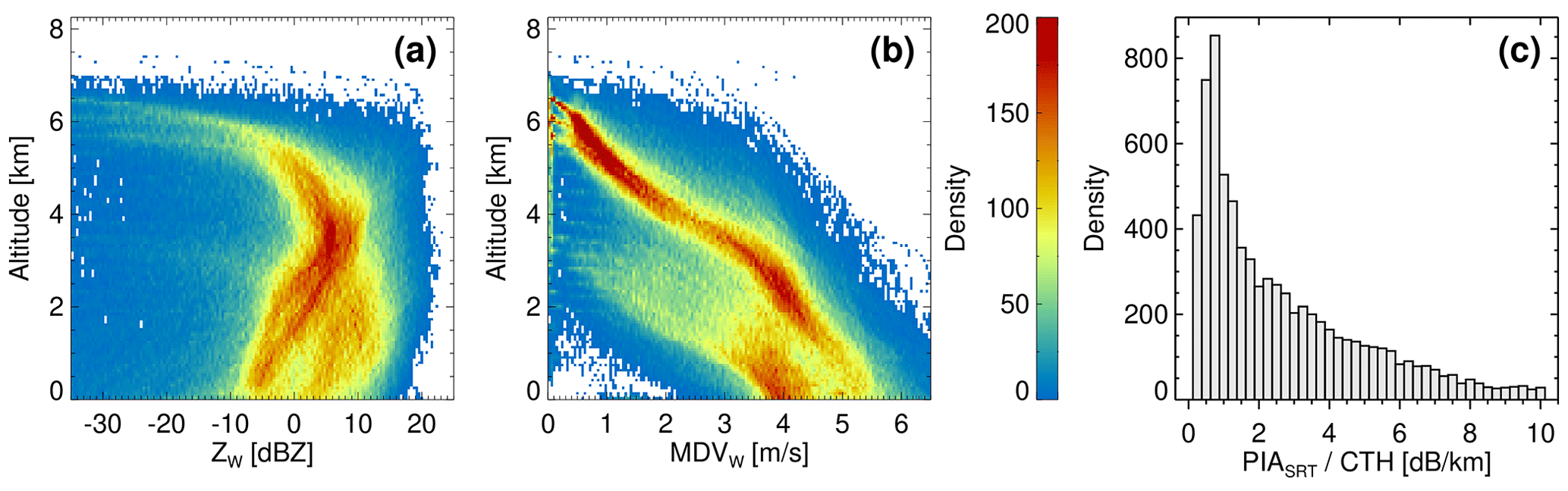
Figure 2Contour frequency altitude diagrams of the (a) radar reflectivity (ZW) and (b) mean Doppler velocity (MDVW) of the warm-rain profiles used for the C-CLD validation. Panel (c) shows a histogram of the PIASRT estimates (one-way) normalized by the cloud top height (CTH).
Validation of the retrieval was performed using approximately 8000 warm-rain columns, and its performance is illustrated in Fig. 3. The algorithm accuracy and precision are quantified by the mean error (ME) and root mean square error (RMSE) in the retrieved variables. The correlation coefficient (r) and normalized RMSE , where SD(x) denotes the standard deviation of x) are computed as additional quality metrics. Since the considered variables are given in the logarithmic units, i.e. log 10CLWP, log 10MC and log 10Dm, the ME and RMSE are given in bels (B). On average, the algorithm is overestimating the liquid cloud water path by about 32 % ( B and 100.12≈1.32). For profiles with higher cloud water content, the overestimation is reduced but scattered more around the 1–1 line. An opposite behaviour is observed for rain; the algorithm underestimates the rain MC by approximately 26 % (ME=0.13 B and ) to compensate for the PIA overestimation due to the cloud droplets. The retrieval of Dm shows very good accuracy; for mm, the algorithm tends to underestimate the characteristic size only by 5 % ( B). Because the same forward model was used for the retrieval and the scene simulations, the systematic underestimation for large sizes is believed to be caused by non-uniform beam-filling (NUBF) effects; i.e. the antenna-pattern-averaged mean Doppler velocity is smaller than the Doppler velocity corresponding to the footprint-averaged Dm because of the shadowing effect due to attenuation in correspondence to the fraction of the footprint with larger reflectivities (see Fig. 9 in Mroz et al., 2018). The precision of the algorithm is greatly reduced when PIA estimates are not assimilated in the retrieval, which is reflected in a reduction in the correlation coefficient and an increase in the RMSE values, as can be seen in Fig. 3d and e. The RMSE value increases from 0.24 and 0.27 to 0.48 and 0.45 B, while the correlation drops from 0.81 and 0.94 to 0.31 and 0.76 for CWP and rain MC, respectively. The estimate of the characteristic size is not affected by the lack of PIA measurements because it is mainly retrieved from the Doppler velocity measurements.
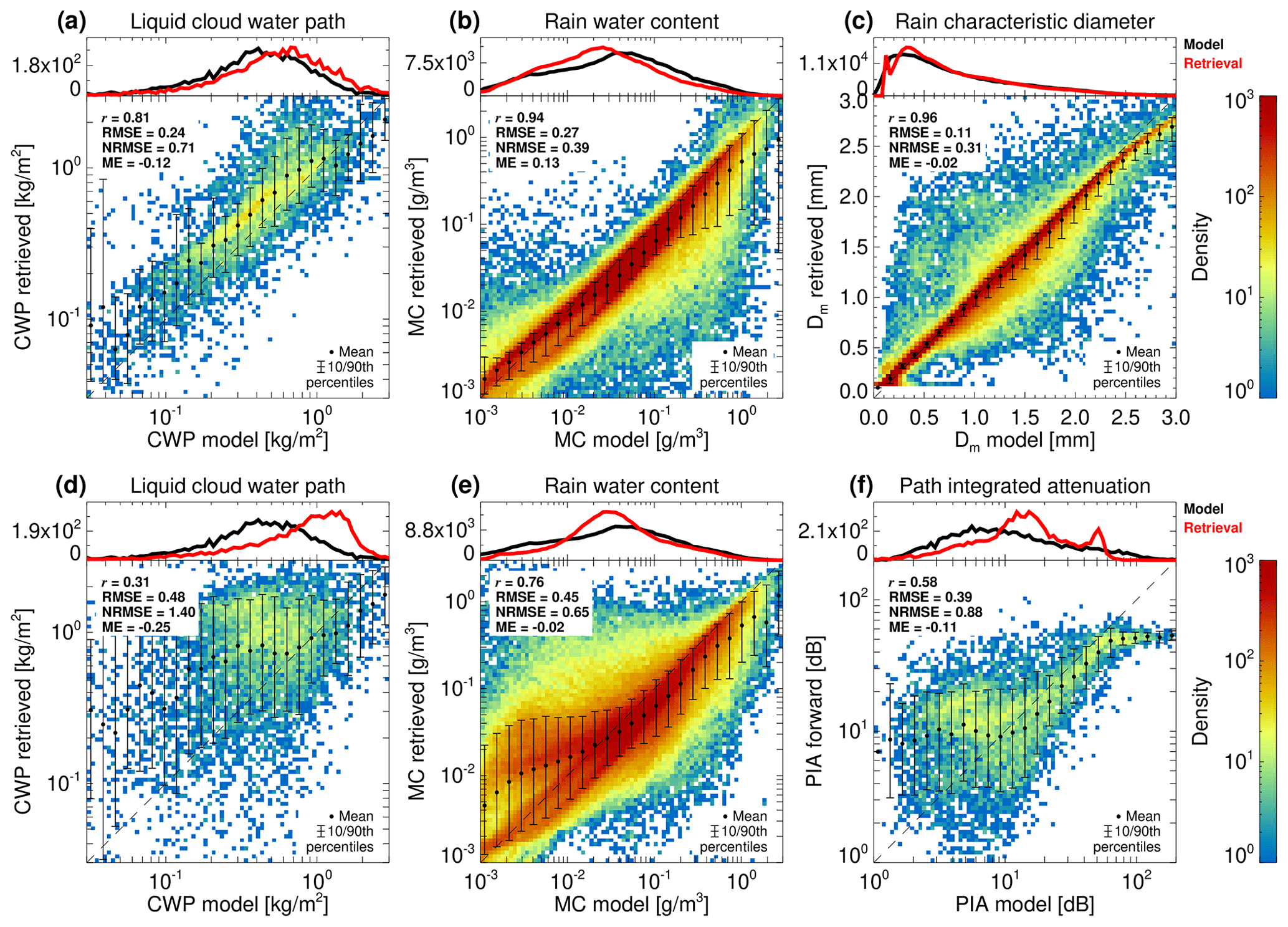
Figure 3The warm-rain algorithm performance histograms. The x axis represents the model values, while the y axis corresponds to the retrieval. Panels (a), (b) and (c) show the cloud liquid water path, rain water content and rain characteristic diameter, respectively. Panels (d), (e) and (f) show the cloud liquid water path, rain water content and forward path-integrated attenuation when assuming that the PIA is not available. The reported values of the ME, RMSE, normalized RMSE (NRMSE) and correlation coefficient (r) are calculated for unknowns in the logarithmic units, i.e. log 10CLWP, log 10MC and log 10Dm.
When PIA measurements are available, the simulated PIA is practically the same as the one being assimilated, with small differences due to the assumed error in the PIA measurements (i.e. 1 dB), giving a correlation of 0.99 and RMSE of 0.07 dB. When the PIA measurements are not available, the algorithm estimates the PIA using the maximum value of the reflectivity profile and the value close to the surface. While this approximation is useful, the lack of an integral constraint makes the correlation between measured and retrieved PIA drop to 0.58 and the RMSE increase to 0.39 dB as shown in Fig. 3f. When raindrops are present in the CPR radar sampling volume, they dominate the CPR observables. In this case, the information provided by the radar reflectivity and mean Doppler velocity is not sufficient to predict the PIA values reported by the model well. This results in a tendency to overestimate the amount of liquid cloud water content and thus to overestimate the observed attenuation.
The quality of the mass content retrieval can be further improved when the PIA estimate based on the surface reference technique (Eq. 32) is corrected for NUBF. We quantify this by replacing the PIASRT estimate with the fine-scale antenna-pattern-averaged attenuation values. In that case, the bias and RMSE in the rain MC estimate are reduced by 14 percentage points for both metrics. This indicates the need for more research on the NUBF and the related forward model adjustments, even in the case of satellite systems with such small footprints as the EarthCARE CPR (Battaglia et al., 2020a).
3.2 Cold rain and snow
The cold-rain and snow retrieval was applied to all the simulated scenes; in Fig. 4 the “Halifax” scene over eastern Canada is presented (for more detail on the simulated scenes, see Donovan et al., 2023). The left-hand side panels show the model output, while the right-hand side panels depict the retrieval and the simulated radar observables. The first part of the scene is occupied by light and moderate snow, with the cloud tops below 5 km. The second part presents ice clouds reaching 8 km and the associated stratiform precipitation with the melting layer between 2 and 3 km a.s.l., clearly highlighted by a sharp change in the Doppler signal. The cold-rain part features a heavy precipitation band associated with convection where the rain rates exceed 10 mm h−1.
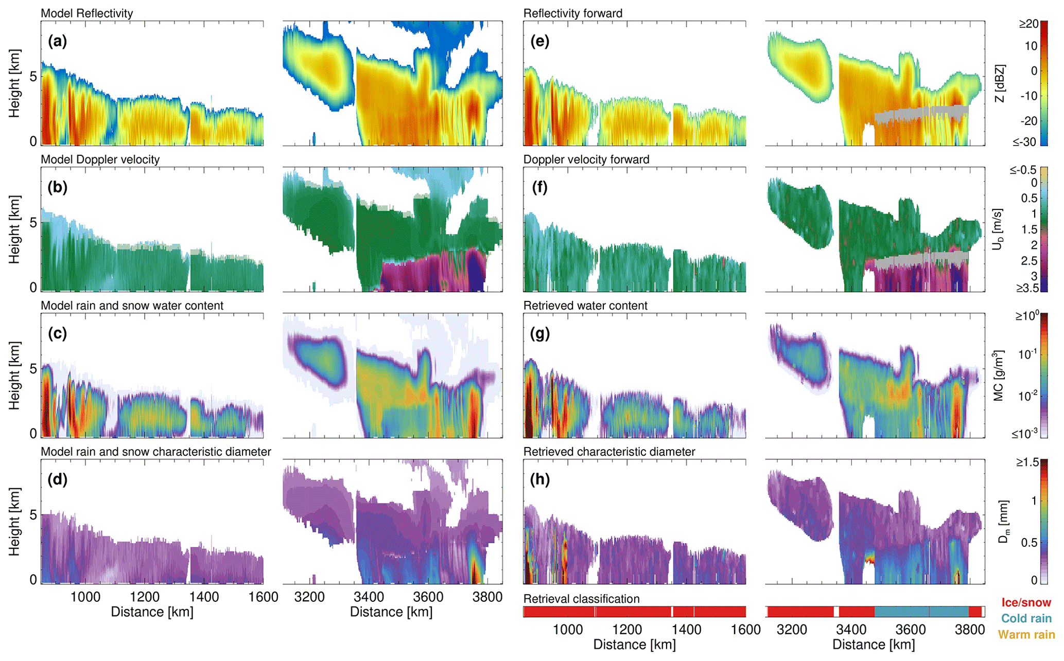
Figure 4Panels (a), (b), (c) and (d) show the model radar reflectivity, Doppler velocity, mass content and mean-mass-weighted characteristic diameter for the ice and cold-rain regions of the Halifax scene. Panels (e), (f), (g) and (h) show the forward radar reflectivity and Doppler velocity and the retrieved mass content and mean-mass-weighted characteristic diameter applied to all regions, where dBZ. The grey band represents the melting layer where the retrieval is not applied.
Overall, the C-CLD algorithm reliably reproduces the radar measurements corresponding to the precipitation structure, and despite being designed for stratiform rain, it performs relatively well even for convective profiles characterized by moderate precipitation conditions. The largest differences between the simulations and the retrieval within the stratiform rain systems are observed around the along-track distance of 3450 km close to the ground. The problem that affects these profiles is a misclassification in the C-TC product of pixels with a mixture of ice and rain as pure-snow columns. This leads to erroneously large Dm estimates and failure of the algorithm. The worst performance of the algorithm is observed for the retrieval of Dm in snow. Due to limited information content about the density of ice in the instrument illuminated volume, different degrees of riming tested by the algorithm can provide comparable cost function values. Therefore, the choice of the final solution may not be entirely accurate. Future work on the algorithm should focus on including such ambiguities in the final uncertainty estimates of the state vector.
Statistics on the retrieval accuracy based on all the scenes are presented in Fig. 5. The results for snow microphysical parameters combine the solid-phase part of cold-rain profiles and pure-snow profiles. These statistics correspond to radar reflectivity values in excess of −21 dBZ, where Doppler velocity is considered reliable, and the retrieval shows a full potential of Z and UD measurements. The snow MC retrieval is strongly correlated with the model output, with a slight tendency to underestimate. The reported RMSE of 0.23 B corresponds to a fractional uncertainty of 53 %. The retrieval of Dm is more ambiguous (which is reflected in higher values of NRMSE) due to the limited variability in Doppler measurements with snow size, especially in the case of low-density ice (Fig. A2). Moreover, due to non-Rayleigh effects the reflectivity is not a monotonic function of the size, which additionally hampers the retrieval. This results in a moderate correlation coefficient of 0.68. As expected, the sizing retrieval in rain has a higher correlation and lower RMSE values than in ice due to the tighter relationship between the size and mean Doppler velocity. Like in the case of warm rain, the algorithm underestimates sizes above 0.6 mm and underestimates the MC values. However, in cold rain these differences are more pronounced because, in addition to NUBF effects, they are amplified by differences between the forward model used in retrieval and the one used in GEM simulations (not shown). Our forward model provides higher Doppler velocity for sizes exceeding 0.7 mm and smaller velocities below this size, which explains differences in the retrieved size. These differences propagate further into the MC retrieval. For Dm<0.7 mm the radar reflectivity increases with size, so an overestimate in Dm causes negative bias in the MC retrieval. When Dm>0.7 mm, reflectivity decreases, and thus the MC is underestimated also for large raindrops.
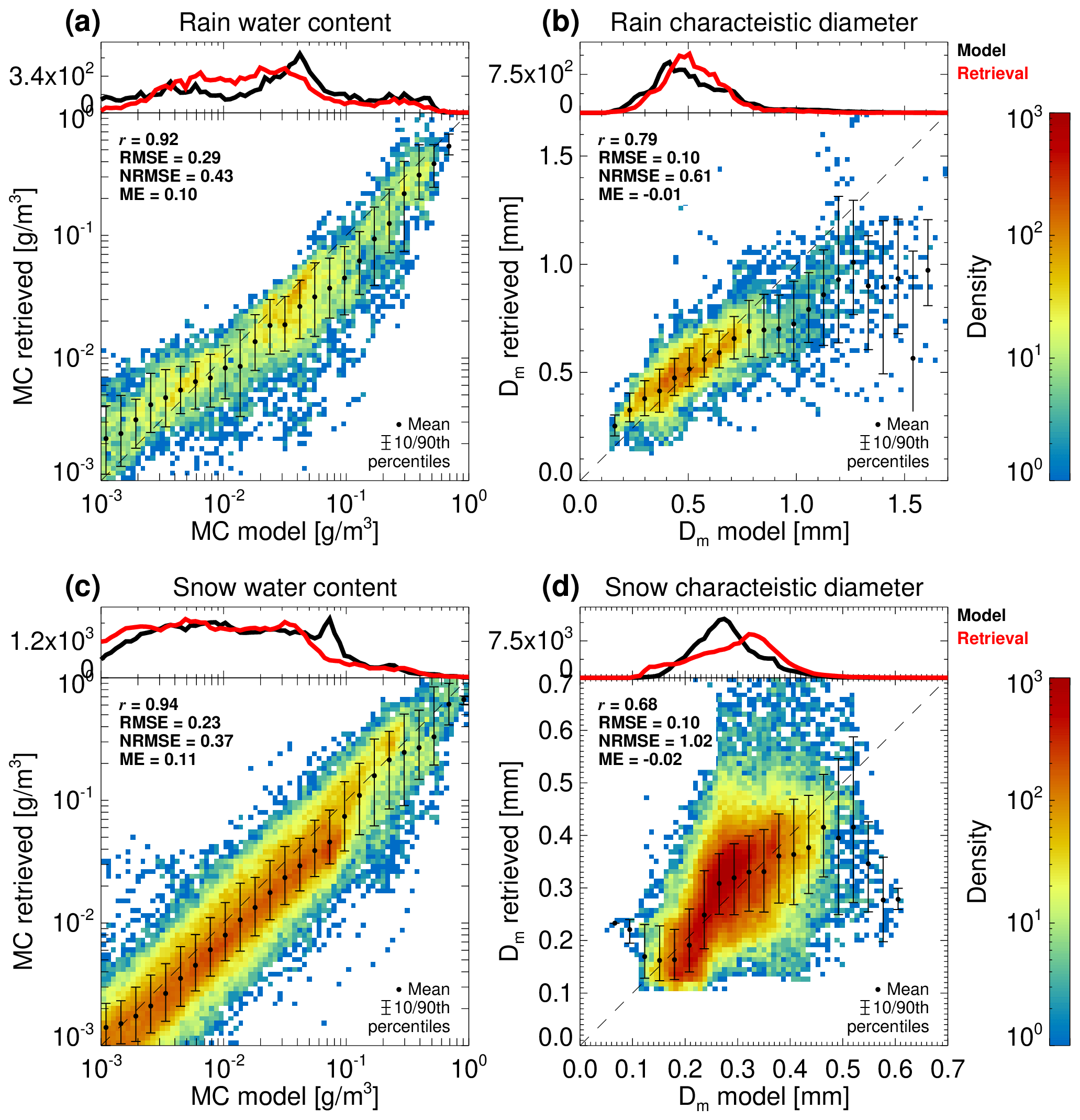
Figure 5The algorithm performance histograms based on the three GEM scenes. The x axis represents the model values, while the y axis corresponds to the retrieval. Panels (a) and (b) show the rain water content and rain characteristic diameter. Panels (c) and (d) show the snow water content and snow characteristic diameter. The profiles with significant contributions of graupel and hail and the regions at cloud tops where the measurements are not very well constrained (large UD error) are excluded from the analysis.
3.3 Stability and sensitivity of the optimal estimation biases in the measurements, the forward model and the a priori estimate
The calibration of radar systems and correct assumptions on microphysics are paramount for the accuracy of remote sensing retrievals. This is presented in Fig. 6, where the precision of the C-CLD algorithm in rain with various error sources is tested. The quality of the retrieval is quantified in terms of the NRMSE. First, the sensitivity of the retrieval to biases in the measurements is tested by adding a constant offset in the forward model to the radar reflectivity and the Doppler velocity. Note that this is equivalent to adding a bias with an opposite sign to the measurements; thus the calibration errors and model biases are tested simultaneously. As expected, the retrieval of the MC is mainly affected by the biases in the reflectivity, which is manifested in the valley-like shape of a local minimum, with the RMSE changing mainly along log 10MC direction. Having said that, some compensation effects are also observed; i.e. the RMSE shows little variability if Z and UD are simultaneously increased or decreased according to the direction given by the valley shape as shown in Fig. 6a. This is due to the characteristics of the forward model, namely the fact that the reflectivity depends on both the size and the mass content of rain. Thus, for a fixed mass, deviations in the reflectivity are compensated for by changes in Dm corresponding to changes in the Doppler velocity. The accuracy of the retrieval of log 10Dm is also driven mainly by one variable, the mean Doppler velocity. As for the other unknowns, biases in the Doppler velocity measurements can be, at least to a certain degree, compensated by an offset in the reflectivity. However, due to a very constrained relation between Dm and UD, the compensation is not as effective as for the MC retrieval and is mainly driven by the Z–Dm relationship used for the a priori estimate.
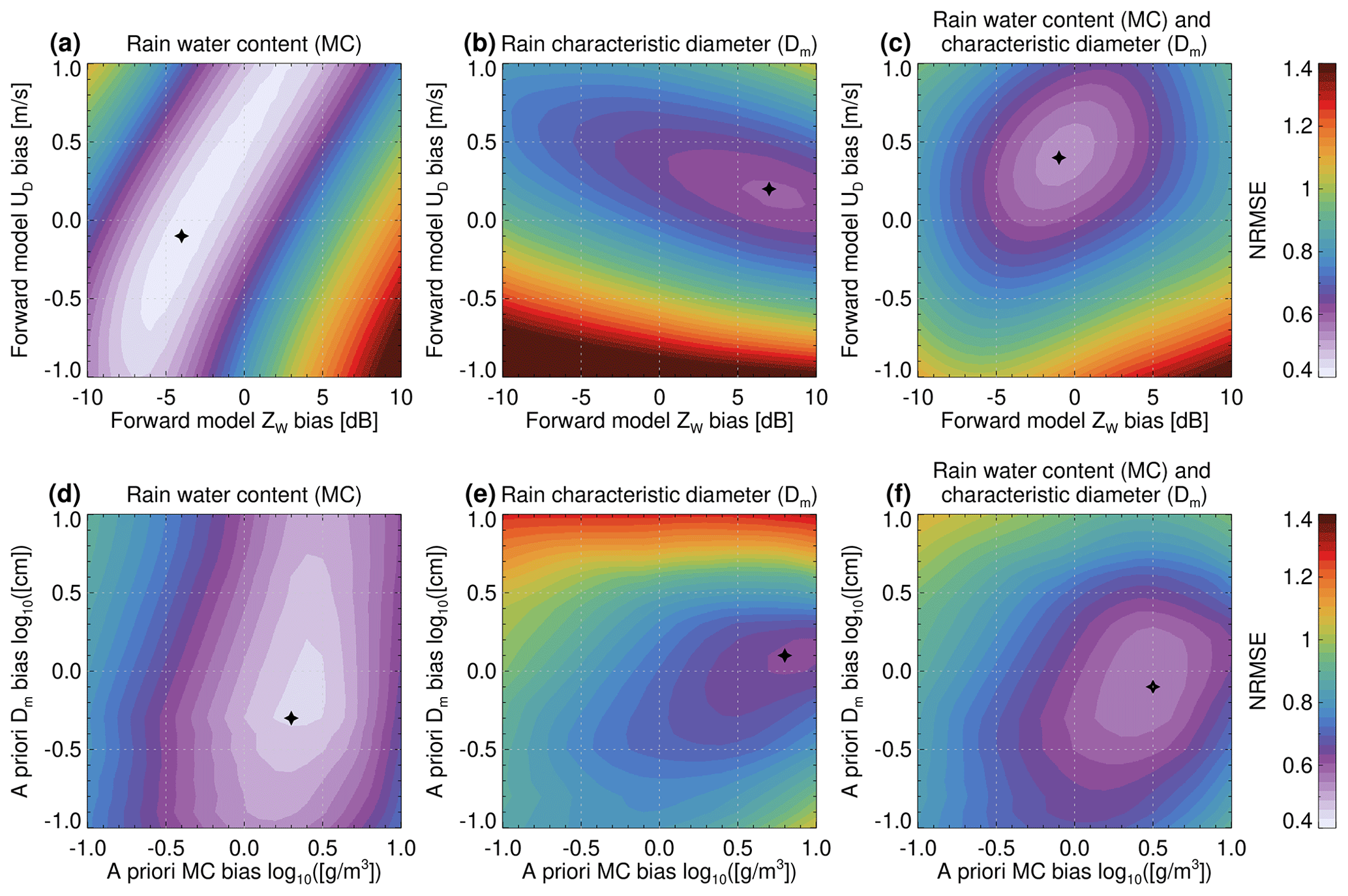
Figure 6The accuracy of the C-CLD algorithm applied to the Halifax scene quantified by the NRMSE of Dm and MC. This evaluation takes into account the impact of (a, b, c) radar simulator bias and (d, e, f) a priori assumption bias in MC and Dm estimates. Panels (c) and (f) display the average NRMSE values for MC and Dm. The cross symbolizes the location of the minimum NRMSE.
The position of a local minimum of the average of the NRMSE in log 10Dm and log 10MC indicates the “reference” point that provides the best possible retrieval. As can be seen, the minimum is shifted away from the origin, which indicates differences between the forward model used in the retrieval and the one used for simulations. An offset of 0.4 m s−1 and −1 dB in UD and Z, respectively, would improve the reported retrieval uncertainties, but we decided not to alter our radar simulator as there is no evidence of the GEM model assumptions being superior to those used in the retrieval.
A similar analysis was performed to quantify the effect of the a priori assumption on the quality of the retrieval. As expected, the retrieval of Dm is mainly affected by its a priori estimate, and the same applies to the retrieval of MC. The error in the MC estimation resulting from differences between forward models (or calibration errors) can be reduced by changing the a priori assumptions, and the optimal retrieval is obtained if log 10MC is increased by approximately 0.5 (i.e. a factor of 3.2). This indicates that for a given reflectivity value in rain, the mean mass content in the GEM model is larger than our a priori estimate. It raises the question of whether the Z–MC relationship, based on the PSD measurements at the ground (which typically fail in detecting small raindrops and low rain rates), which provides the basis of our forward model, is applicable in the low-precipitation-rate regime (Z<10 dBZ) that constitutes the majority of the profiles tested here.
3.4 The added value of the Doppler measurements
The EarthCARE radar mission is a follow-up of the highly successful CloudSat spaceborne radar mission. A number of studies on clouds and precipitation properties were conducted based on the CloudSat measurements (Stephens et al., 2018; Luo et al., 2008; Matrosov and Heymsfield, 2008; Tourville et al., 2015). The EarthCARE CPR is more sensitive (5–6 dB); has better vertical and horizontal sampling; has a smaller instantaneous field of view; and, most of all, has Doppler measurement capabilities. With all of these assets, it is vital to determine what improvement in the understanding of the properties of precipitation and clouds will be brought by the new mission.
The analysis presented here focuses on the Doppler velocity measurements value and their impact on the retrieval. The evaluation is based on comparison of the retrieval statistics with and without Doppler information assimilation. For this purpose, the C-CLD algorithm is applied once more to the Halifax scene, this time assuming no Doppler measurements. As expected, this results in reduced quality of the characteristic-size estimate. In rain, the correlation coefficient between Dm from the model and the retrieved one drops from 0.79 (for the original algorithm) to 0.47 in the no-Doppler setting. Similarly, the RMSE is approximately doubled for the reduced-input retrieval. This decreased confidence in the size estimate propagates to the retrieval of the rain water content, and it results in an RMSE increase from 0.29 to 0.44 B. The correlation drops from 0.92 to 0.79. Importantly, the lack of velocity measurements has no effect on the accuracy of the retrievals, with the mean error being almost non-affected.
The restriction of the measurement vector to radar reflectivity only has a small effect on the retrieval in the snow/ice. The RMSE and the ME statistics are virtually unchanged. Having said that, the correlation coefficient of the snow characteristic size decreases from 0.68 to 0.36 for no-Doppler retrieval. All the retrieved sizes oscillate in a narrow range of values between 0.2 and 0.3 mm that corresponds to the a priori estimates for the range of the observed reflectivities. This shows that Doppler measurements are relevant to estimating the size of snowflakes. Insignificant differences in the RMSE values between the size retrievals with and without velocity observations are due to the relative uncertainty in the velocity observations; i.e. the assumed measurement uncertainty of 0.2 m s−1 gives a large fractional uncertainty in snow, where falling velocity often does not exceed 1 m s−1.
One of the advantages of OE algorithms is the ability to quantify the amount of information provided by an individual measurement. This is achieved by comparing the state vector uncertainties before and after the measurements are assimilated by the algorithm (Shannon and Weaver, 1949). In geometrical terms, the information content of an observation is defined as the ratio between the volume enclosed by 1 standard deviation of the prior and posterior probability density function of X. For Gaussian distributions, this can be computed as follows:
where denotes the determinant of a matrix and Rx and Ra are posterior and prior covariance matrices defined in Sect. 2.2.3 (see Eq. 2.73 in Rodgers, 2000). The computation of (Eq. 18) for different instrument configurations does not require multiple runs of the computationally expensive algorithm. Instead, once the retrieval has converged, the diagonal elements of the matrix that correspond to selected measurements can be set to 0 to mimic instrument shutdown. This allows for the quantification of information content for all measurements together, for just radar reflectivity or just Doppler velocity or even for a single measurement at a given height in the column as shown in Fig. 7b and c.
To ensure a fair comparison among various regimes, the subsequent analysis focuses solely on quantifying the information content of the measurement in relation to estimates of mass content and characteristic size. Factors such as a reduction in uncertainty in melting layer attenuation or liquid cloud water content are not taken into consideration, as these variables are not present in all OE retrievals.
The amount of information provided by EarthCARE CPR measurements varies depending on the size and type of the hydrometeor being observed. In general, radar reflectivity provides more information for ice and snow, while mean Doppler velocity is more informative for rain. This trend is particularly noticeable in cold-rain columns, where the information content of reflectivity decreases from 3.2 to 2.5 nat (natural unit of information) as the hydrometeor transitions from a solid to liquid phase. In contrast, the information content of Doppler velocity increases from 2 to 2.5 nat during the same transition. The Doppler velocity measurements are useful for decreasing uncertainty in precipitation size estimation, particularly in rain, where the information content can surpass 2.5 nat. In snow, the observed sedimentation velocities have a smaller dynamic range, which results in reduced information content. High information content of radar reflectivity in ice can be attributed to an effective reduction in the uncertainty in the ice water content.
The amount of information is not uniform for a given measurement or hydrometeor type, as it depends also on the precipitation size. This non-uniformity in the information content is most apparent in warm-rain profiles, but it is also evident if rain pixels from Halifax simulations are compared with the “Cabo Verde” scene, where the retrieved sizes tend to be larger. In the case of reflectivity in warm rain, the information content is the highest at the top of the precipitation column, where particles are smaller than approximately 0.8 mm. Then, it reaches a minimum at the raindrop size that is the most efficient for the backscattering radar reflectivity signal (see the radar reflectivity maximum in Fig. A1a). For sizes larger than 0.8–0.9 mm, the information content is approximately 2 nat. A similar behaviour is observed for Doppler velocity but with a less pronounced minimum at 1 mm, where a reduction in the slope of UD is observed. The maximum in the information content is observed for Dm=0.4 mm.
The total amount of information available from EarthCARE CPR measurements ranges from 3 to 4.4 nat, depending on factors such as hydrometeor type, ice-to-rain layer thickness ratio and particle size. Upon analysis of individual components, it is evident that, in snow and cold rain, the radar reflectivity profile (with PIA) provides the most information out of all measurements considered. It is followed by the Doppler velocity profile, as demonstrated in Fig. 7d. In contrast, in warm rain, both reflectivity and velocity measurements carry a similar amount of information. This trend also applies when considering only the liquid-phase precipitation in cold-rain profiles, as can be seen in the lower portion of Fig. 7b and c.
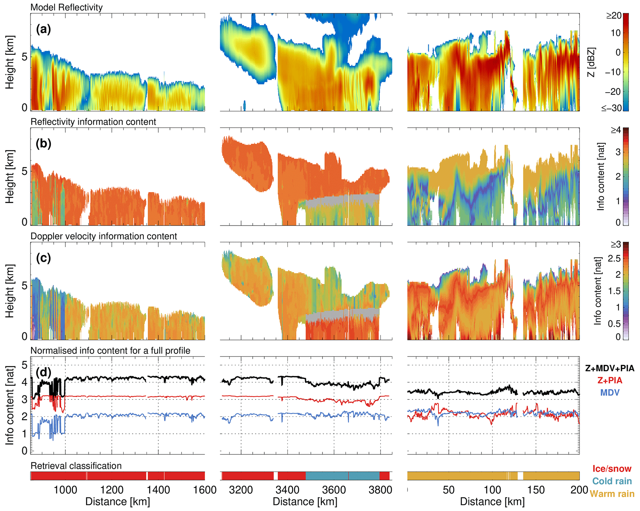
Figure 7Information content for different measurements. Panel (a) shows the radar reflectivity for the context. Panel (b) displays the information content for individual measurements of radar reflectivity in the column. Similarly, panel (c) shows information content for individual measurements of Doppler velocity, and panel (d) shows the information content of an entire profile of measurements, as indicated in the legend. To ensure consistency across the different profiles, the information content values have been normalized by the number of retrieval levels.
The analysis presented here shows that the Doppler measurements are particularly valuable in remote sensing retrievals because they offer additional information that complements the measurements of reflectivity and PIA. In fact, the information content from all measurements combined () is typically about 1 nat greater than the information content of reflectivity and PIA alone, demonstrating the significance of Doppler observations. That said, it is important to note that the information content of Z and PIA summed with the information content of UD is larger than the information content of all measurements. Thus, there is some overlap between the information content of Doppler velocity and reflectivity, and they are not entirely independent. Furthermore, it is interesting to note that the information content of Doppler velocity is comparable for all considered regimes, while the reflectivity measurements are more advantageous in ice and cold rain.
The cloud and precipitation microphysics (C-CLD) algorithm is an EarthCARE Level 2 (L2) data product that utilizes measurements from the EarthCARE 94 GHz Doppler Cloud Profiling Radar (CPR) to provide microphysical information about cloud and precipitation systems. The C-CLD algorithm primarily uses an optimal estimation (OE) approach that balances the information provided by the CPR with a priori knowledge on the climatology of cloud and precipitation systems. The algorithm is designed to retrieve profiles of two moments of the PSD drop size, namely the mass content and mean-mass-weighted diameter, owing to the information content provided by the CPR. When dealing with drizzle-free and lightly drizzling warm clouds, the OE framework is replaced with climatological relationships between the measured reflectivities and the microphysical parameters of interest.
A large dataset of in situ, surface-based observations is used to reduce the number of free parameters and to obtain the forward model relations with the corresponding uncertainties. To maintain water mass flux through the melting layer, only small perturbations from this condition are allowed. Additionally, a one-dimensional parameterization is proposed for representing a wide range of ice particle densities, from unrimed snowflakes to dense graupel particles.
The C-CLD retrieval framework has been applied to EarthCARE CPR simulated observations from high-resolution weather systems simulations occurring in three different climatological regimes (Donovan et al., 2023): tropical climate, humid continental climate bordering on an oceanic climate (Halifax) and mid-latitude conditions over North America (Baja). The CPR reflectivity and Doppler radar measurements provide sufficient information to retrieve, with high confidence, two moments of the PSD, especially in rain due to the added value of the Doppler measurements, which, in stratiform rain, are closely related to the raindrop fall speed and thus to its mean size. On average, the mean-mass-weighted diameter (Dm) of rain can be estimated within a precision of 23 % with negative bias reported for large sizes. As a result, the estimate of rain mass content (MC) is also captured well by matching the radar reflectivity to the observations. The uncertainty in the MC estimate is estimated to be 67 % for all the GEM simulation scenes combined. Despite more complex and ambiguous scattering properties of ice particles, errors in the ice mass content are smaller than in rain, and they are equal to 53 % for profiles including either snow-only or cold rain. This unexpected result may indicate differences in the forward model used in GEM simulations and in the retrieval of rain or difficulties in separating path-integrated attenuation (PIA) into the liquid cloud, melting layer and rain components. The retrieval of Dm of ice is the most challenging; it is characterized by the lowest correlation coefficient and the highest value of the normalized root mean square error among all the considered unknowns. The variety of snowflake morphology and the corresponding diversity in the relation between particle size and terminal velocity results in uncertainties of 23 %.
Due to the high susceptibility of W-band measurements to signal attenuation, the quality of the retrieval is strongly reduced when the path-integrated attenuation estimates are not assimilated. This is reflected in the degradation of the quality of the mass content retrieval in warm-rain conditions; i.e. the RMSE in log 10MC increases from 0.27 to 0.45 B, while the correlation coefficient is reduced from 0.97 to 0.75.
The reported uncertainties are heavily dependent on the forward model accuracy and on the measurement calibration biases. The performed analysis revealed that, due to some differences in the fall velocities used in the GEM model and in the C-CLD retrieval framework, a systematic overestimation (underestimation) of small (large) raindrop sizes is present. These errors, combined with discrepancies in the reflectivity forward model, result in a negative bias of the rain mass content. The differences between the simulators are attributed to the different particle size distribution shape assumptions. Although the difference between the radar simulators was not systematic (i.e. it has a different sign depending on the rain characteristic size), the bias in the mass content retrieval was. This shows how susceptible to model and/or measurement biases the optimal estimation framework is and how important the calibration of the EarthCARE reflectivity and Doppler velocity (Battaglia and Kollias, 2014) will be.
Despite the detection of differences between the GEM simulations and our radar model, the algorithm was not fine-tuned to match model assumptions due to the lack of evidence that the model could reflect reality better than the long-term particle size distribution statistics. This paper aims at providing a physical basis for the retrieval, and so the modifications of the forward model or of a priori assumptions are left for the calibration–validation activity period after the launch of the satellite.
Thanks to its large antenna, CPR's unprecedented fine horizontal resolution minimizes the impact of two of the challenges of spaceborne radar-based precipitation remote sensing: multiple scattering (Battaglia et al., 2010; Matrosov et al., 2008; Matrosov and Battaglia, 2009) and non-uniform beam filling (NUBF; Tanelli et al., 2012). Since the horizontal resolution of the model simulations is finer than the one of the radar, errors related to NUBF are quantified and included in the reported total algorithm errors, with small biases observed. Furthermore, negligible multiple scattering effects were simulated and reported to the flag produced in C-PRO (Kollias et al., 2022b).
The CloudSat mission radar measurements and the information about clouds and precipitation derived from them provide a strong heritage for the C-CLD product development. However, this legacy poses a challenge for consistency of the retrieved parameters for the two missions. Continuity between the products is important for evaluation of the long-term trends in precipitation statistics and climate change studies. To address this issue, the information content of Doppler measurements and their impact on the retrieval must be carefully evaluated. The knowledge about the cloud and precipitation properties gained with this additional measurement can be transferred to the reflectivity-only algorithm via refinement of the a priori assumptions. The updated C-CLD algorithm (i.e. without Doppler measurements and considering differences in the instrument specifications) can be applied to the CloudSat measurements and compared to its products for an assessment of potential biases. In the case of detection of systematic differences, the CloudSat dataset can be reprocessed to provide a consistent long-term cloud and precipitation record.
Our preliminary analysis shows that the amount of information provided by EarthCARE CPR measurements varies depending on the size and type of hydrometeor observed, with reflectivity more informative for ice and snow and mean Doppler velocity for rain. The Doppler velocity measurements are particularly useful in reducing uncertainty in precipitation size estimation, especially for rain. The non-uniformity in the information content is most apparent in warm-rain profiles, where the size of particles is evolving with height. The maximum in the information content of UD is observed for Dm=0.4 mm. The analysis reveals that the Doppler measurements complement the measurements of reflectivity and PIA, and the information content of all measurements combined is typically about 1 nat greater than the information content of reflectivity and PIA alone.
Further development of the algorithm is necessary to ensure its effectiveness in a wider range of weather conditions. The GEM simulations used in this study do not include weather systems with raindrops or snowflakes larger than 1 mm. These conditions are particularly challenging for W-band retrievals due to significant signal attenuation and saturation of radar reflectivity and Doppler measurements (Mróz et al., 2019). To improve the credibility of a priori estimates in the drizzle size particle regime, more in situ measurements are required. This aspect should be addressed during the calibration–validation activities. Moreover, characterizing the shape of the liquid cloud mass content profiles is essential for reducing uncertainties in path-integrated attenuation simulations and retrieved rain and snow mass content below the liquid cloud top. As suggested by Battaglia and Panegrossi (2020), this issue can be mitigated by the inclusion of the W-band brightness temperatures in the observables adopted in the derivation of the C-FMR product. In addition, in order to produce realistic transitions in the retrieved state vector between consecutive profiles, future algorithms could make use of the two-dimensional information provided by the radar. In addition, future algorithms could leverage the two-dimensional information from the radar to create seamless transitions between consecutive profiles. This not only preserves the horizontal continuity of the state vector but also enables accurate quantification and correction of NUBF effects. Additionally, using a two-dimensional approach can aid in detecting liquid clouds that may be present within precipitation. These clouds typically have long correlation lengths and are easier to spot outside of precipitation zones where larger hydrometeors are not masking them. Once these clouds are detected in these areas, their location within precipitation can be inferred through continuity. Finally, future work should include cross-validation with the other precipitation products, e.g. ACM-CAP (Mason et al., 2023), which provides a synergistic retrieval of the hydrometeor properties based on the full suite of sensors on board the EarthCARE satellite. This latter product should provide more accurate estimates due to the increased information content provided by the other instruments.
Here, we report the parameterizations of the scattering properties at 94 GHz that are used in C-CLD. These relations link the CPR observables (reflectivity Ze and Doppler velocity UD) with two state vector parameters (Dm and MC) in terms of power laws. This simplifies the analytical computation of the Jacobian.
A1 Rain
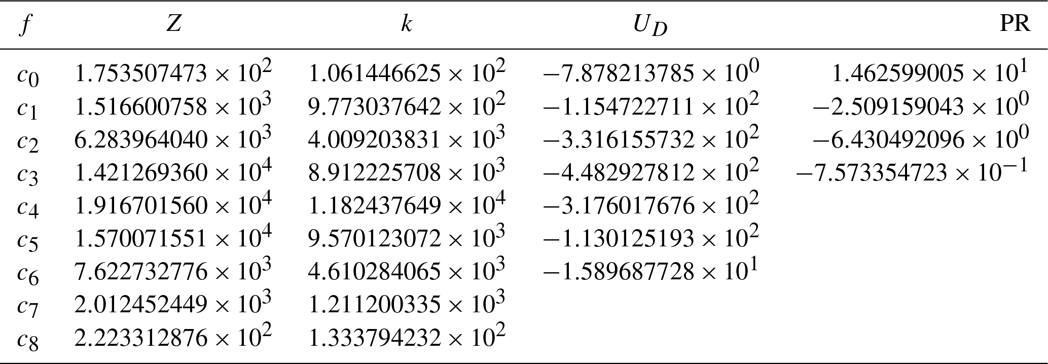
The radar observables and PSD moments are approximated by polynomials in and y=log 10Dm[cm], i.e.
where the coefficients for and PR are given in Table A1. The degree of the fitting polynomial results from its high accuracy in replicating the simulations for the gamma PSD model over a broad range of characteristic rain sizes, i.e. from 0.1 to 3.5 mm.
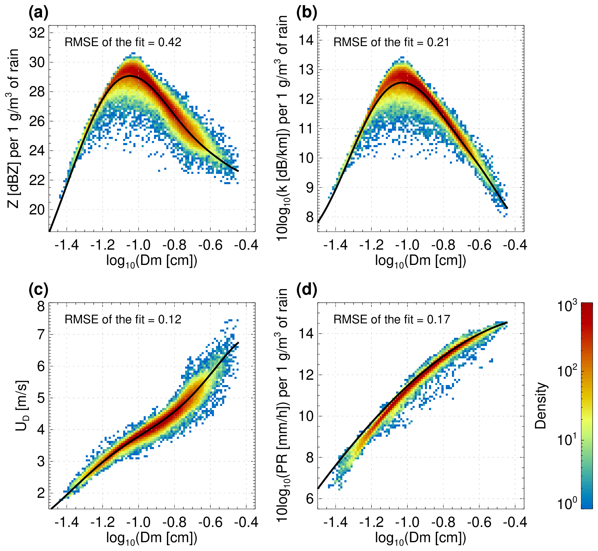
Figure A1Two-dimensional histograms of the radar-observable simulations corresponding to the in situ PSD measurements at the ground. (a) Radar reflectivity factor in dBZ per 1 g m−3 of rain. (b) 10log 10 of the (one-way) specific attenuation in dB km−1 per 1 g m−3 of rain. (c) Mean Doppler velocity in standard atmospheres. (d) Precipitation rate in standard atmospheric conditions (15 ∘C, 1013.25 mbar) per 1 g m−3 of rain. The black line shows the simulations for the gamma PSD model with that is used as a forward model.
A2 Cloud attenuation coefficients
The two-way attenuation coefficient in dB km−1 g−1 m3 is parameterized as a quadratic function of the temperature expressed in Celsius with the zeroth-, the first- and the second-order coefficients equal to . This replicates the empirically verified model at 94 GHz very well (Tridon et al., 2020, Fig. 1) with a maximum of about 8.5 dB km−1 g−1 m3 at 271.8 K decreasing to 7 dB km−1 g−1 m3 at 245.7 and at 297.8 K.
A3 Ice
As in the case of rain, the radar observables and PSD moments are approximated by polynomials in and y=log 10Dm [cm]. These polynomials are of different degrees, and their coefficients depend on the degree of riming. Therefore, it is impractical to list all the coefficients here. Instead, these tables are freely available at https://doi.org/10.5281/zenodo.7529739 (Mroz, 2023). Figure A2 shows the scattering properties as parameterized in the forward model for five selected degrees of riming. Note that while attenuation and Doppler velocities tend to increase with melted diameter, reflectivities reach maximum values in correspondence to sizes between 0.4 and 0.8 mm.
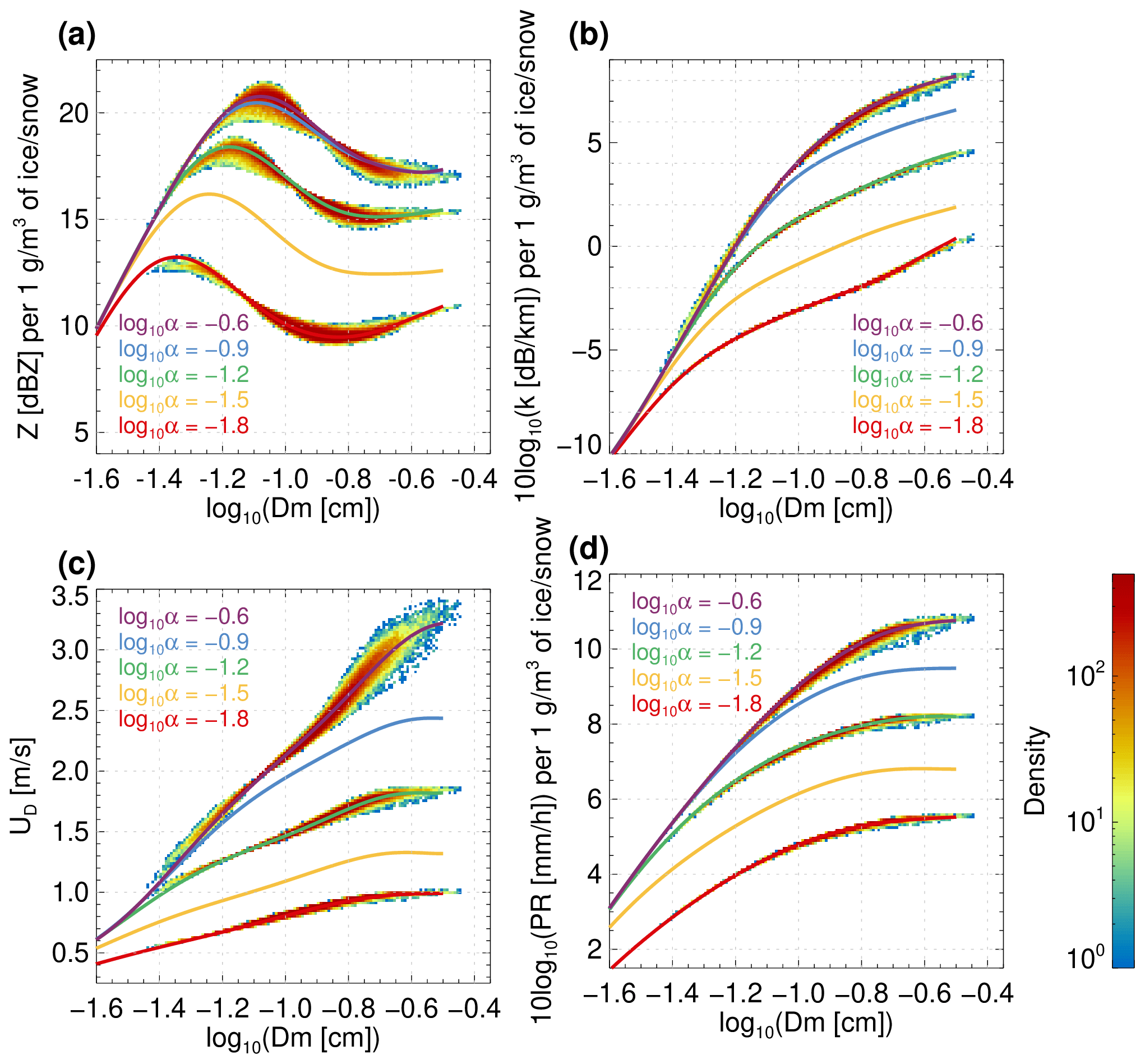
Figure A2Ice-scattering properties as parameterized in the forward model as a function of the equivalent melted size; different colours correspond to different degrees of riming (α). For selected values of α, the histograms in the background show the gamma PSD modelling corresponding to the rain PSD measurements collected at the ground based on the “melting-only” assumption (see Sect. 2.4.1). The line represents . All the simulations are performed for 1 g m−3 of snow. (a) Radar reflectivity factor is in decibels relative to Z. (b) 10log 10 of the (one-way) specific attenuation is in decibels per kilometre. (c) Mean Doppler velocity is in standard atmospheres. (d) Precipitation rate is in standard atmospheres.
The vertical gradient of the change in adiabatic LWC is calculated as in Rogers and Yau (1989) and is parameterized as
with = .
The EarthCARE Level 2 demonstration products from simulated scenes, including the C-CLD product discussed in this paper, are available from https://doi.org/10.5281/zenodo.7311704 (van Zadelhoff et al., 2022). The dataset of single-scattering properties of large snow aggregates used in this study is available at https://doi.org/10.5281/zenodo.7510186 (Mroz and Leinonen, 2023). Parametrization of scattering properties in the W-band for a population of ice particles is available at https://doi.org/10.5281/zenodo.7529739 (Mroz, 2023).
KM led the preparation of the paper and developed the retrieval scheme. KM and BPT performed the analysis presented here. AB and PK advised on the methodology of the algorithm. BPT and AT led the Fortran implementation of the algorithm. BPT generated all the figures. FT contributed to the development of the W-band radar simulator. The manuscript was written by KM, BPT, AB and PK.
The contact author has declared that none of the authors has any competing interests.
Publisher's note: Copernicus Publications remains neutral with regard to jurisdictional claims in published maps and institutional affiliations.
This article is part of the special issue “EarthCARE Level 2 algorithms and data products”. It is not associated with a conference.
Work done by Kamil Mroz and Alessandro Battaglia was performed under a contract with the National Centre for Earth Observation. This research used the ALICE High Performance Computing facility at the University of Leicester. Work done by Bernat Puidgomènech Treserras and Pavlos Kollias was supported by the European Space Agency (ESA) under the Clouds, Aerosol, Radiation – Development of INtegrated ALgorithms (CARDINAL) project.
This research has been supported by the European Space Agency (grant no. RFQ/3-17010/20/NL/AD) and the National Centre for Earth Observation (grant no. RP18G0088).
This paper was edited by Robin Hogan and reviewed by two anonymous referees.
Baedi, R., de Wit, J., Russchenberg, H., Erkelens, J., and Poiares Baptista, J.: Estimating effective radius and liquid water content from radar and lidar based on the CLARE98 data-set, Phys. Chem. Earth Pt. B, 25, 1057–1062, https://doi.org/10.1016/S1464-1909(00)00152-0, 2000. a
Battaglia, A. and Kollias, P.: Using ice clouds for mitigating the EarthCARE Doppler radar mispointing, IEEE T. Geosci. Remote, 53, 2079–2085, https://doi.org/10.1109/TGRS.2014.2353219, 2014. a
Battaglia, A. and Panegrossi, G.: What Can We Learn from the CloudSat Radiometric Mode Observations of Snowfall over the Ice-Free Ocean?, Remote Sens.-Basel, 12, 3285, https://doi.org/10.3390/rs12203285, 2020. a
Battaglia, A., Tanelli, S., Kobayashi, S., Zrnic, D., Hogan, R. J., and Simmer, C.: Multiple-scattering in radar systems: A review, J. Quant. Spectrosc. Ra., 111, 917–947, https://doi.org/10.1016/j.jqsrt.2009.11.024, 2010. a
Battaglia, A., Mroz, K., Lang, T., Tridon, F., Tanelli, S., Tian, L., and Heymsfield, G. M.: Using a multiwavelength suite of microwave instruments to investigate the microphysical structure of deep convective cores, J. Geophys. Res.-Atmos., 121, 9356–9381, https://doi.org/10.1002/2016JD025269, 2016. a
Battaglia, A., Kollias, P., Dhillon, R., Lamer, K., Khairoutdinov, M., and Watters, D.: Mind the gap – Part 2: Improving quantitative estimates of cloud and rain water path in oceanic warm rain using spaceborne radars, Atmos. Meas. Tech., 13, 4865–4883, https://doi.org/10.5194/amt-13-4865-2020, 2020a. a, b
Battaglia, A., Kollias, P., Dhillon, R., Roy, R., Tanelli, S., Lamer, K., Grecu, M., Lebsock, M., Watters, D., Mroz, K., Heymsfield, G., Li, L., and Furukawa, K.: Spaceborne Cloud and Precipitation Radars: Status, Challenges, and Ways Forward, Rev. Geophys., 58, e2019RG000686, https://doi.org/10.1029/2019RG000686, 2020b. a, b, c
Battaglia, A., Tanelli, S., Tridon, F., Kneifel, S., Leinonen, J., and Kollias, P.: Satellite precipitation measurement, in: Adv. Global Change Res., vol. 1, chap. 13: Triple-frequency radar retrievals, Springer, ISBN: 978-3-030-24567-2, 2020c. a
Böhm, J. P.: A general hydrodynamic theory for mixed-phase microphysics. Part I: drag and fall speed of hydrometeors, Atmos. Res., 27, 253–274, https://doi.org/10.1016/0169-8095(92)90035-9, 1992. a
Brandes, E. A., Zhang, G., and Vivekanandan, J.: Corrigendum, J. Appl. Meteorol., 44, 186–186, https://doi.org/10.1175/1520-0450(2005)44<186:C>2.0.CO;2, 2005. a
Brown, P. R. A. and Francis, P. N.: Improved Measurements of the Ice Water Content in Cirrus Using a Total-Water Probe, J. Atmos. Ocean. Tech., 12, 410–414, 1995. a
Burns, D., Kollias, P., Tatarevic, A., Battaglia, A., and Tanelli, S.: The performance of the EarthCARE Cloud Profiling Radar in marine stratiform clouds, J. Geophys. Res.-Atmos., 121, 14525–14537, https://doi.org/10.1002/2016JD025090, 2016. a
Cole, J. N. S., Barker, H. W., Qu, Z., Villefranque, N., and Shephard, M. W.: Broadband Radiative Quantities for the EarthCARE Mission: The ACM-COM and ACM-RT Products, Atmos. Meas. Tech. Discuss. [preprint], https://doi.org/10.5194/amt-2022-304, in review, 2022. a
Côté, J., Gravel, S., Méthot, A., Patoine, A., Roch, M., and Staniforth, A.: The operational CMC–MRD global environmental multiscale (GEM) model. Part I: Design considerations and formulation, Mon. Weather Rev., 126, 1373–1395, https://doi.org/10.1175/1520-0493(1998)126<1373:TOCMGE>2.0.CO;2, 1998. a
Delanoë, J., Protat, A., Testud, J., Bouniol, D., Heymsfield, A. J., Bansemer, A., Brown, P. R. A., and Forbes, R. M.: Statistical properties of the normalized ice particle size distribution, J. Geophys. Res., 110, D10201, https://doi.org/10.1029/2004JD005405, 2005. a
Delanoë, J., Protat, A., Bouniol, D., Heymsfield, A., Bansemer, A., and Brown, P.: The Characterization of Ice Cloud Properties from Doppler Radar Measurements, J. Atmos. Sci., 46, 1682–1698, https://doi.org/10.1175/JAM2543.1, 2007. a
Dolan, B., Fuchs, B., Rutledge, S. A., Barnes, E. A., and Thompson, E. J.: Primary Modes of Global Drop Size Distributions, J. Atmos. Sci., 75, 1453–1476, https://doi.org/10.1175/JAS-D-17-0242.1, 2018. a
Donovan, D. P., Kollias, P., Velázquez Blázquez, A., and van Zadelhoff, G.-J.: The Generation of EarthCARE L1 Test Data sets Using Atmospheric Model Data Sets, EGUsphere [preprint], https://doi.org/10.5194/egusphere-2023-384, 2023. a, b
Eisinger, M., Wehr, T., Kubota, T., Bernaerts, D., and Wallace, K.: The EarthCARE Mission – Science Data Processing Chain Overview, Atmos. Meas. Tech., in preparation, 2023. a
Erfani, E. and Mitchell, D. L.: Growth of ice particle mass and projected area during riming, Atmos. Chem. Phys., 17, 1241–1257, https://doi.org/10.5194/acp-17-1241-2017, 2017. a
Foote, G. B. and du Toit, P. S.: Terminal Velocity of Raindrops Aloft, J. Appl. Meteorol., 8, 249–253, 1969. a
Fox, N. I. and Illingworth, A. J.: The Retrieval of Stratocumulus Cloud Properties by Ground-Based Cloud Radar, J. Appl. Meteorol., 36, 485–492, https://doi.org/10.1175/1520-0450(1997)036<0485:TROSCP>2.0.CO;2, 1997. a
Frisch, A. S., Feingold, G., Fairall, C. W., Uttal, T., and Snider, J. B.: On cloud radar and microwave radiometer measurements of stratus cloud liquid water profiles, J. Geophys. Res., 103, 23195–23198, https://doi.org/10.1029/98JD01827, 1998. a
Girard, C., Desgagné, M., McTaggart-Cowan, R., Côté, J., Charron, M., Gravel, S., Lee, V., Patoine, A., Qaddouri, A., Roch, M., Spacek, L., Tanguay, M., Vaillancourt, P., and Zadra, A.: Staggered vertical discretization of the Canadian environmental multiscale (GEM) model using a coordinate of the log-hydrostatic-pressure type, Mon. Weather Rev., 142, 1183–1196, https://doi.org/10.1175/MWR-D-13-00255.1, 2014. a
Gunn, R. and Kintzer, G. D.: The terminal velocity of fall for water droplets in stagnant air, J. Meteorol., 6, 243–248, https://doi.org/10.1175/1520-0469(1949)006<0243:TTVOFF>2.0.CO;2, 1949. a
Guyot, A., Pudashine, J., Protat, A., Uijlenhoet, R., Pauwels, V. R. N., Seed, A., and Walker, J. P.: Effect of disdrometer type on rain drop size distribution characterisation: a new dataset for south-eastern Australia, Hydrol. Earth Syst. Sci., 23, 4737–4761, https://doi.org/10.5194/hess-23-4737-2019, 2019. a
Haynes, J. M., L'Ecuyer, T. S., Stephens, G. L., Miller, S. D., Mitrescu, C., Wood, N. B., and Tanelli, S.: Rainfall retrieval over the ocean with spaceborne W-band radar, J. Geophys. Res., 114, D00A22, https://doi.org/10.1029/2008JD009973, 2009. a, b
Heymsfield, A. J.: A Comparative Study of the Rates of Development of Potential Graupel and Hail Embryos in High Plains Storms, J. Atmos. Sci., 39, 2867–2897, https://doi.org/10.1175/1520-0469(1982)039<2867:ACSOTR>2.0.CO;2, 1982. a
Heymsfield, A. J., Protat, A., Bouniol, D., Austin, R. T., Hogan, R. J., Delanoë, J., Okamoto, H., Sato, K., van Zadelhoff, G.-J., Donovan, D. P., and Wang, Z.: Testing IWC Retrieval Methods Using Radar and Ancillary Measurements with In Situ Data, J. Appl. Meteorol. Clim., 47, 135–163, https://doi.org/10.1175/2007JAMC1606.1, 2008. a
Hitschfeld, W. and Bordan, J.: Errors inherent in the radar measurement of rainfall at attenuating wavelengths, J. Meteorol., 11, 58–67, https://doi.org/10.1175/1520-0469(1954)011<0058:EIITRM>2.0.CO;2, 1954. a, b, c, d
Hogan, R. J.: A variational scheme for retrieving rainfall rate and hail reflectivity fraction from polarization radar, J. Appl. Meteorol., 46, 1544–1564, https://doi.org/10.1175/JAM2550.1, 2006. a
Hogan, R. J. and Westbrook, C. D.: Equation for the microwave backscatter cross section of aggregate snowflakes using the Self-Similar Rayleigh-Gans Approximation, J. Atmos. Sci., 71, 3292–3301, https://doi.org/10.1175/JAS-D-13-0347.1, 2014. a
Hou, A. Y., Kakar, R. K., Neeck, S., Azarbarzin, A. A., Kummerow, C. D., Kojima, M., Oki, R., Nakamura, K., and Iguchi, T.: The Global Precipitation Measurement Mission, B. Am. Meteorol. Soc., 95, 701–722, https://doi.org/10.1175/BAMS-D-13-00164.1, 2014. a
Illingworth, A. J., Hogan, R. J., Connor, E. J. O., Bouniol, D., Brooks, M. E., Delanoë, J., Donovan, P., Eastment, J. D., Gaussiat, N., Goddard, J. W. F., Haeffelin, M., Baltink, H. K., Krasnov, O. A., Pelon, J., Piriou, J.-M., Protat, A., Russchenberg, H. W. J., Seifert, A., Tompkins, A. M., van Zadelhoff, G.-J., Vinit, F., Willen, U., Wilson, D. R., and Wrench, C. L.: CLOUDNET: continuous evaluation of cloud profiles in seven operational models using ground-based observations, B. Am. Meteorol. Soc., 88, 883–898, https://doi.org/10.1175/BAMS-88-6-883, 2007. a, b
Illingworth, A. J., Barker, H. W., Beljaars, A., Ceccaldi, M., Chepfer, H., Clerbaux, N., Cole, J., Delanoë, J., Domenech, C., Donovan, D. P., Fukuda, S., Hirakata, M., Hogan, R. J., Huenerbein, A., Kollias, P., Kubota, T., Nakajima, T., Nakajima, T. Y., Nishizawa, T., Ohno, Y., Okamoto, H., Oki, R., Sato, K., Satoh, M., Shephard, M. W., Velázquez-Blázquez, A., Wandinger, U., Wehr, T., and van Zadelhoff, G.-J.: The EarthCARE Satellite: The Next Step Forward in Global Measurements of Clouds, Aerosols, Precipitation, and Radiation, B. Am. Meteorol. Soc., 96, 1311–1332, https://doi.org/10.1175/BAMS-D-12-00227.1, 2015. a, b
Kalesse, H. and Kollias, P.: Climatology of High Cloud Dynamics Using Profiling ARM Doppler Radar Observations, J. Climate, 26, 6340–6359, https://doi.org/10.1175/JCLI-D-12-00695.1, 2013. a
Kneifel, S., Leinonen, J., Tyynela, J., Ori, D., and Battaglia, A.: Satellite precipitation measurement, in: Adv. Global Change Res., vol. 1, chap. 15: Scattering of Hydrometeors, Springer, ISBN: 978-3-030-24567-2, 2020. a
Kollias, P., Albrecht, B. A., and Marks, F.: Why Mie? Accurate Observations of Vertical Air Velocities and Raindrops Using a Cloud Radar, B. Am. Meteorol. Soc., 83, 1471–1483, https://doi.org/10.1175/BAMS-83-10-1471, 2002. a
Kollias, P., Jo, I., Borque, P., Tatarevic, A., Lamer, K., Bharadwaj, N., Widener, K., Johnson, K., and Clothiaux, E. E.: Scanning ARM Cloud Radars. Part II: Data Quality Control and Processing, J. Atmos. Ocean. Tech., 31, 583–598, https://doi.org/10.1175/JTECH-D-13-00045.1, 2014. a
Kollias, P., Bharadwaj, N., Clothiaux, E. E., Lamer, K., Oue, M., Hardin, J., Isom, B., Lindenmaier, I., Matthews, A., Luke, E. P., Giangrande, S. E., Johnson, K., Collis, S., Comstock, J., and Mather, J. H.: The ARM Radar Network: At the Leading-edge of Cloud and Precipitation Observations, B. Am. Meteorol. Soc., 101, E588–E607, https://doi.org/10.1175/BAMS-D-18-0288.1, 2020. a, b
Kollias, P., Battaglia, A., Lamer, K., Treserras, B. P., and Braun, S. A.: Mind the Gap – Part 3: Doppler Velocity Measurements From Space, Frontiers in Remote Sensing, 3, 860284, https://doi.org/10.3389/frsen.2022.860284, 2022a. a
Kollias, P., Puidgomènech Treserras, B., Battaglia, A., Borque, P., and Tatarevic, A.: Processing reflectivity and Doppler velocity from EarthCARE’s cloud profiling radar: the C-FMR, C-CD and C-APC products, EGUsphere [preprint], https://doi.org/10.5194/egusphere-2022-1284, 2022b. a, b, c, d, e, f
Kruger, A. and Krajewski, W. F.: Two-Dimensional Video Disdrometer: A Description, J. Atmos. Ocean. Tech., 19, 602–617, 2002. a
Lamer, K., Puigdomènech Treserras, B., Zhu, Z., Isom, B., Bharadwaj, N., and Kollias, P.: Characterization of shallow oceanic precipitation using profiling and scanning radar observations at the Eastern North Atlantic ARM observatory, Atmos. Meas. Tech., 12, 4931–4947, https://doi.org/10.5194/amt-12-4931-2019, 2019. a, b
Lebsock, M. D. and L'Ecuyer, T. S.: The retrieval of warm rain from CloudSat, J. Geophys. Res., 116, D20209, https://doi.org/10.1029/2011JD016076, 2011. a, b
Leinonen, J. and Szyrmer, W.: Radar signatures of snowflake riming: A modeling study, Earth Space Sci., 2, 346–358, https://doi.org/10.1002/2015EA000102, 2015. a
Leinonen, J., Lebsock, M. D., Stephens, G. L., and Suzuki, K.: Improved Retrieval of Cloud Liquid Water from CloudSat and MODIS, J. Appl. Meteorol. Clim., 55, 1831–1844, https://doi.org/10.1175/JAMC-D-16-0077.1, 2016. a, b
Löhnert, U. and Crewell, S.: Accuracy of cloud liquid water path from ground-based microwave radiometry. Part I. Dependency on Cloud model statistics, Radio Sci., 38, 8041, https://doi.org/10.1029/2002RS002654, 2003. a
Luo, Z., Stephens, G. L., Emanuel, K. A., Vane, D. G., Tourville, N., and Haynes, J.: On the Use of CloudSat and data for estimating Hurricane Intensity, IEEE Geosci. Remote S., 5, 13–16, https://doi.org/10.1109/LGRS.2007.905341, 2008. a
Mason, S., Hogan, R. J., Donovan, D., van Zadelhoff, G.-J., Kollias, P., Tresseras, B. P., Qu, Z., Cole, J., Hünerbein, A., and Docter, N.: An intercomparison of EarthCARE cloud, aerosol and precipitation retrieval products, Atmos. Meas. Tech., in preparation, 2023. a
Mason, S. L., Chiu, J. C., Hogan, R. J., and Tian, L.: Improved rain rate and drop size retrievals from airborne Doppler radar, Atmos. Chem. Phys., 17, 11567–11589, https://doi.org/10.5194/acp-17-11567-2017, 2017. a
Mason, S. L., Chiu, C. J., Hogan, R. J., Moisseev, D., and Kneifel, S.: Retrievals of Riming and Snow Density From Vertically Pointing Doppler Radars, J. Geophys. Res.-Atmos., 123, 13807–13834, https://doi.org/10.1029/2018JD028603, 2018. a
Mason, S. L., Hogan, R. J., Bozzo, A., and Pounder, N. L.: A unified synergistic retrieval of clouds, aerosols and precipitation from EarthCARE: the ACM-CAP product, EGUsphere [preprint], https://doi.org/10.5194/egusphere-2022-1195, 2022. a
Mather, J. H. and Voyles, J. W.: The ARM climate research facility: a review of structure and capabilities, B. Am. Meteorol. Soc., 94, 377–392, https://doi.org/10.1175/BAMS-D-11-00218.1, 2013. a, b
Matrosov, S.: Assessment of Radar Signal Attenuation Caused by the Melting Hydrometeor Layer, IEEE T. Geosci. Remote, 46, 1039–1047, https://doi.org/10.1109/TGRS.2008.915757, 2008. a, b
Matrosov, S. Y. and Battaglia, A.: Influence of multiple scattering on CloudSat measurements in snow: a model study, Geophys. Res. Lett., 36, L12806, https://doi.org/10.1029/2009GL038704, 2009. a
Matrosov, S. Y. and Heymsfield, A. J.: Estimating ice content and extinction in precipitating cloud systems from CloudSat radar measurements, J. Geophys. Res., 113, D00A05, https://doi.org/10.1029/2007JD009633, 2008. a, b
Matrosov, S. Y. and Heymsfield, A. J.: Empirical Relations between Size Parameters of Ice Hydrometeor Populations and Radar Reflectivity, J. Appl. Meteorol. Clim., 56, 2479–2488, https://doi.org/10.1175/JAMC-D-17-0076.1, 2017. a
Matrosov, S. Y. and Turner, D. D.: Retrieving Mean Temperature of Atmospheric Liquid Water Layers Using Microwave Radiometer Measurements, J. Atmos. Ocean. Tech., 35, 1091–1102, https://doi.org/10.1175/JTECH-D-17-0179.1, 2018. a
Matrosov, S. Y., Battaglia, A., and Rodriguez, P.: Effects of Multiple Scattering on Attenuation-Based Retrievals of Stratiform Rainfall from CloudSat, J. Atmos. Ocean. Tech., 25, 2199–2208, https://doi.org/10.1175/2008JTECHA1095.1, 2008. a
Milbrandt, J., Bélair, S., Faucher, M., Vallée, M., Carrera, M. A., and Glazer, A.: The Pan-Canadian High Resolution (2.5 km) Deterministic Prediction System, Weather Forecast., 31, 1791–1816, https://doi.org/10.1175/WAF-D-16-0035.1, 2016. a
Miles, N. L., Verlinde, J., and Clothiaux, E. E.: Cloud Droplet Size Distributions in Low-Level Stratiform Clouds, J. Atmos. Sci., 57, 295–311, https://doi.org/10.1175/1520-0469(2000)057<0295:CDSDIL>2.0.CO;2, 2000. a, b, c
Moisseev, D., von Lerber, A., and Tiira, J.: Quantifying the effect of riming on snowfall using ground-based observations, J. Geophys. Res.-Atmos., 122, 4019–4037, https://doi.org/10.1002/2016JD026272, 2017. a
Morrison, H. and Milbrandt, J. A.: Parameterization of cloud microphysics based on the prediction of bulk ice particle properties. Part I: Scheme description and idealized tests, J. Atmos. Sci., 72, 287–311, https://doi.org/10.1175/JAS-D-14-0065.1, 2015. a
Morrison, H., Thompson, G., and Tatarskii, V.: Impact of Cloud Microphysics on the Development of Trailing Stratiform Precipitation in a Simulated Squall Line: Comparison of One- and Two-Moment Schemes, Mon. Weather Rev., 137, 991–1007, https://doi.org/10.1175/2008MWR2556.1, 2009. a
Mroz, K.: Single Scattering properties at W-band of ice populations, Version 0.1, Zenodo [data set], https://doi.org/10.5281/zenodo.7529739, 2023. a, b
Mroz, K. and Leinonen, J.: Microwave Single Scattering Properties Database (Horizontally Aligned Aggregates of Dendrites), Version 1.0, Zenodo [data set], https://doi.org/10.5281/zenodo.7510186, 2023. a, b
Mroz, K., Battaglia, A., Lang, T. J., Tanelli, S., and Sacco, G. F.: Global Precipitation Measuring Dual-Frequency Precipitation Radar Observations of Hailstorm Vertical Structure: Current Capabilities and Drawbacks, J. Appl. Meteorol. Clim., 57, 2161–2178, https://doi.org/10.1175/JAMC-D-18-0020.1, 2018. a
Mróz, K., Battaglia, A., Kneifel, S., D'Adderio, L. P., and Dias Neto, J.: Triple-frequency Doppler retrieval of characteristic raindrop size, Earth Space Sci., 7, e2019EA000789, https://doi.org/10.1029/2019EA000789, 2019. a, b
Mróz, K., Battaglia, A., Kneifel, S., von Terzi, L., Karrer, M., and Ori, D.: Linking rain into ice microphysics across the melting layer in stratiform rain: a closure study, Atmos. Meas. Tech., 14, 511–529, https://doi.org/10.5194/amt-14-511-2021, 2021a. a
Mroz, K., Battaglia, A., Nguyen, C., Heymsfield, A., Protat, A., and Wolde, M.: Triple-frequency radar retrieval of microphysical properties of snow, Atmos. Meas. Tech., 14, 7243–7254, https://doi.org/10.5194/amt-14-7243-2021, 2021b. a
Oue, M., Kollias, P., Shapiro, A., Tatarevic, A., and Matsui, T.: Investigation of observational error sources in multi-Doppler-radar three-dimensional variational vertical air motion retrievals, Atmos. Meas. Tech., 12, 1999–2018, https://doi.org/10.5194/amt-12-1999-2019, 2019. a
Protat, A., Delanoë, J., Bouniol, D., Heymsfield, A. J., Bansemer, A., and Brown, P.: Evaluation of Ice Water Content Retrievals from Cloud Radar Reflectivity and Temperature Using a Large Airborne In Situ Microphysical Database, J. Appl. Meteorol. Clim., 46, 557–572, https://doi.org/10.1175/JAM2488.1, 2007. a
Protat, A., Rauniyar, S., Delanoë, J., Fontaine, E., and Schwarzenboeck, A.: W-Band (95 GHz) Radar Attenuation in Tropical Stratiform Ice Anvils, J. Atmos. Ocean. Tech., 36, 1463–1476, https://doi.org/10.1175/JTECH-D-18-0154.1, 2019. a
Qu, Z., Korolev, A., Milbrandt, J. A., Heckman, I., Huang, Y., McFarquhar, G. M., Morrison, H., Wolde, M., and Nguyen, C.: The impacts of secondary ice production on microphysics and dynamics in tropical convection, Atmos. Chem. Phys., 22, 12287–12310, https://doi.org/10.5194/acp-22-12287-2022, 2022. a, b
Rodgers, C. D.: Inverse methods for atmospheric sounding: theory and practice, World Scientific, River Edge, NJ, 238 pp., https://doi.org/10.1142/3171, 2000. a, b, c
Rogers, R. R. and Yau, M. K.: A short course in cloud physics, Butterworth-Heinemann, Woburn, MA, USA, 290 pp., ISBN: 9780080570945, 1989. a
Sauvageot, H. and Omar, J.: Radar Reflectivity of Cumulus Clouds, J. Atmos. Ocean. Tech., 4, 264–272, https://doi.org/10.1175/1520-0426(1987)004<0264:RROCC>2.0.CO;2, 1987. a
Schulte, R. M., Kummerow, C. D., Klepp, C., and Mace, G. G.: How Accurately Can Warm Rain Realistically Be Retrieved with Satellite Sensors? Part I: DSD Uncertainties, J. Appl. Meteorol. Clim., 61, 1087–1105, https://doi.org/10.1175/JAMC-D-21-0158.1, 2022. a
Shannon, C. E. and Weaver, W.: The Mathematical Theory of Communication, University of Illinois Press, Urbana, IL, ISBN 10: 0252725468, 1949. a
Stephens, G., Winker, D., Pelon, J., Trepte, C., Vane, D., Yuhas, C., LÉcuyer, T., and Lebsock, M.: CloudSat and CALIPSO within the A-Train: Ten Years of Actively Observing the Earth System, B. Am. Meteorol. Soc., 99, 569–581, https://doi.org/10.1175/BAMS-D-16-0324.1, 2018. a, b
Stephens, G. L., Vane, D. G., Boain, R. J., Mace, G. G., Sassen, K., Wang, Z., Illingworth, A. J., O'connor, E. J., Rossow, W. B., Durden, S. L., Miller, S. D., Austin, R. T., Benedetti, A., and Mitrescu, C. A.: THE CLOUDSAT MISSION AND THE A-TRAIN, B. Am. Meteorol. Soc., 83, 1771–1790, https://doi.org/10.1175/BAMS-83-12-1771, 2002. a
Stephens, G. L., L'Ecuyer, T., Forbes, R., Gettelmen, A., Golaz, J.-C., Bodas-Salcedo, A., Suzuki, K., Gabriel, P., and Haynes, J.: Dreary state of precipitation in global models, J. Geophys. Res., 115, D24211, https://doi.org/10.1029/2010JD014532, 2010. a
Stephens, G. L., Li, J., Wild, M., Clayson, C., Loeb, N., Kato, S., L'Ecuyer, T., Stackhouse, P., Lebsock, M., and Andrews, T.: An update on Earth's energy balance in light of the latest global observations, Nat. Geosci., 5, 691–696, https://doi.org/10.1038/ngeo1580, 2012. a
Szyrmer, W., Tatarevic, A., and Kollias, P.: Ice clouds microphysical retrieval using 94-GHz Doppler radar observations: Basic relations within the retrieval framework, J. Geophys. Res., 117, D14203, 117, https://doi.org/10.1029/2011JD016675, 2012. a
Tanelli, S., Sacco, G. F., Durden, S., and Haddad, Z: Impact of non-uniform beam filling on spaceborne cloud and precipitation radar retrieval algorithms, in: Remote Sensing of the Atmosphere, Clouds, and Precipitation IV, edited by: Hayasaka, T., Nakamura, K., and Im, E., SPIE, 8523, 852308, https://doi.org/10.1117/12.977375, 2012. a
Tourville, N., Stephens, G., DeMaria, M., and Vane, D.: Remote Sensing of Tropical Cyclones: Observations from CloudSat and A-Train Profilers, B. Am. Meteorol. Soc., 96, 609–622, https://doi.org/10.1175/BAMS-D-13-00282.1, 2015. a
Tridon, F., Battaglia, A., Chase, R. J., Turk, F. J., Leinonen, J., Kneifel, S., Mroz, K., Finlon, J., Bansemer, A., Tanelli, S., Heymsfield, A. J., and Nesbitt, S. W.: The Microphysics of Stratiform Precipitation During OLYMPEX: Compatibility Between Triple-Frequency Radar and Airborne In Situ Observations, 124, 8764–8792, https://doi.org/10.1029/2018JD029858, 2019a. a
Tridon, F., Planche, C., Mroz, K., Banson, S., Battaglia, A., Van Baelen, J., and Wobrock, W.: On the Realism of the Rain Microphysics Representation of a Squall Line in the WRF Model. Part I: Evaluation with Multifrequency Cloud Radar Doppler Spectra Observations, Mon. Weather Rev., 147, 2787–2810, https://doi.org/10.1175/MWR-D-18-0018.1, 2019b. a, b
Tridon, F., Battaglia, A., and Kneifel, S.: Estimating total attenuation using Rayleigh targets at cloud top: applications in multilayer and mixed-phase clouds observed by ground-based multifrequency radars, Atmos. Meas. Tech., 13, 5065–5085, https://doi.org/10.5194/amt-13-5065-2020, 2020. a, b
Turner, D. D., Kneifel, S., and Careddu, M. P.: An Improved Liquid Water Absorption Model at Microwave Frequencies for Supercooled Liquid Water Clouds, J. Atmos. Ocean. Tech., 33, 33–44, https://doi.org/10.1175/JTECH-D-15-0074.1, 2016. a
van Zadelhoff, G.-J., Barker, H. W., Baudrez, E., Bley, S., Clerbaux, N., Cole, J. N. S., de Kloe, J., Docter, N., Domenech, C., Donovan, D. P., Dufresne, J.-L., Eisinger, M., Fischer, J., García-Marañón, R., Haarig, M., Hogan, R. J., Hünerbein, A., Kollias, P., Koopman, R., Madenach, N., Mason, S. L., Preusker, R., Puigdomènech Treserras, B., Qu, Z., Ruiz-Saldaña, M., Shephard, M., Velázquez-Blazquez, A., Villefranque, N., Wandinger, U., Wang, P., and Wehr, T.: EarthCARE level-2 demonstration products from simulated scenes, Version 10.01, Zenodo [data set], https://doi.org/10.5281/zenodo.7311704, 2022. a
von Lerber, A., Moisseev, D., Bliven, L. F., Petersen, W., Harri, A.-M., and Chandrasekar, V.: Microphysical Properties of Snow and Their Link to Ze–S Relations during BAECC 2014, J. Appl. Meteorol. Clim., 56, 1561–1582, https://doi.org/10.1175/JAMC-D-16-0379.1, 2017. a, b
Wehr, T., Kubota, T., Tzeremes, G., Wallace, K., Nakatsuka, H., Ohno, Y., Koopman, R., Rusli, S., Kikuchi, M., Eisinger, M., Tanaka, T., Taga, M., Deghaye, P., Tomita, E., and Bernaerts, D.: The EarthCARE Mission – Science and System Overview, EGUsphere [preprint], https://doi.org/10.5194/egusphere-2022-1476, 2023. a
Westbrook, C. D., Ball, R. C., Field, P. R., and Heymsfield, A. J.: Theory of growth by differential sedimentation, with application to snowflake formation, Phys. Rev. E, 70, 021403, https://doi.org/10.1103/PhysRevE.70.021403, 2004. a
Williams, C. R.: Vertical Air Motion Retrieved from Dual-Frequency Profiler Observations, J. Atmos. Ocean. Tech., 29, 1471–1480, https://doi.org/10.1175/JTECH-D-11-00176.1, 2012. a
Williams, C. R., Bringi, V. N., Carey, L. D., Chandrasekar, V., Gatlin, P. N., Haddad, Z. S., Meneghini, R., Munchak, S. J., Nesbitt, S. W., Petersen, W. A., Tanelli, S., Tokay, A., Wilson, A., and Wolff, D. B.: Describing the Shape of Raindrop Size Distributions Using Uncorrelated Raindrop Mass Spectrum Parameters, J. Appl. Meteorol. Clim., 53, 1282–1296, https://doi.org/10.1175/JAMC-D-13-076.1, 2014. a, b
Wood, R., Kubar, T. L., and Hartmann, D. L.: Understanding the Importance of Microphysics and Macrophysics for Warm Rain in Marine Low Clouds. Part II: Heuristic Models of Rain Formation, J. Atmos. Sci., 66, 2973–2990, https://doi.org/10.1175/2009JAS3072.1, 2009. a
- Abstract
- Introduction
- Description of the algorithm
- Validation of the algorithm
- Conclusions
- Appendix A: Parameterization of scattering properties in the W-band
- Appendix B: Other parameterizations
- Data availability
- Author contributions
- Competing interests
- Disclaimer
- Special issue statement
- Acknowledgements
- Financial support
- Review statement
- References