An explicit formulation for the retrieval of the overlap function in an elastic and Raman aerosol lidar

We derive an explicit (i.e., non-iterative) formula for the retrieval of the overlap function in an aerosol lidar with both elastic and Raman N₂ and/or O₂ channels used for independent measurements of aerosol backscatter and extinction coefficients. The formula requires only the measured, range-corrected elastic and the corresponding Raman signals, plus an assumed lidar ratio. We assess the influence of the lidar ratio error in the overlap function retrieval and present retrieval examples.

1 Introduction

At near ranges, lidar signals suffer from a varying overlap between the emitted laser beam and the field of view of the receiving optical assembly. The overlap function of a lidar system can be defined as the ratio between the power scattered by a scattering volume at a given range that reaches the photodetector (excluding transmission losses) and the power scattered by the same scattering volume that reaches the telescope aperture (Comeron et al., 2011). This ratio is a function of range, especially at short ranges, and depends on the optical and geometrical arrangement of the transmitting and receiving optics of the instrument. The key parameters determining the overlap function are those related to the laser beam features (diameter, shape and divergence), receiver optical properties (telescope diameter, focal length and field stop diameter), and relative location and alignment between transmitter and receiver optical axes (Halldórsson and Langerholc, 1978; Lefrère, 1982). In a perfectly aligned system, the overlap function is 0 at the telescope aperture level and progressively grows up to a constant value, where all the backscattered radiation collected by the telescope aperture, or at least a constant proportion of it, reaches the photodetector. In practical cases, misalignments may make the overlap function dependence on range depart from the ideal behavior just described.

The existence of a varying overlap prevents the system from trustfully providing lidar signals for ranges below the altitude at which the overlap attains a constant value, thus limiting the minimum operational range of the lidar instrument. To reduce these overlap issues, some systems duplicate their receivers, enabling both far- and near-range telescopes and detectors and combining their respective signals for reconstructing a lidar signal with an extended (towards the lower end) constant overlap range. For example, Polly^XT systems (Engelmann et al., 2016) use this type of solution, and their full overlap altitude is reduced down to ∼100 m. Alternatives when such a hardware-based extension of the operational range is not possible rely on the calculation or estimation of the overlap function and on the correction of the detected signals from the effect of the varying overlap. Several authors have developed theoretical calculations of the overlap function using the transmitter and the receiver optical parameters, both on an analytical basis (Sassen and Dodd, 1982; Ancellet et al., 1986; Kuze et al., 1998; Stelmaszczyk et al., 2005; Comeron et al., 2011) and by relying on ray-tracing procedures (e.g., Kumar and Rocadenbosch, 2013). However, such theoretical approaches are in many cases not practical because most of the system parameters in which they are based on are not easily measurable (Kokkalis, 2017), and they change, sometimes unpredictably and unnoticeably, with time. Alternatives to theoretical calculations are based on experimental estimations relying on practical field lidar measurements and inversions. A first proposal, presented by Sasano et al. (1979), is based on the assumption of a homogeneous atmosphere up to distances above the full overlap altitude. In many cases, this method is not practical, first, because its applicability depends on the state of the atmosphere and, second, because in order to assure the required atmospheric homogeneity, it demands a horizontal alignment of the lidar line of sight that is not always possible. Further contributions, making different assumptions about the atmospheric conditions, were proposed by Tomine et al. (1989), Dho et al. (1997) and Vande Hey et al. (2011).

A comparison with a reference system not affected (or less affected) by the varying overlap has been proposed by Guerrero-Rascado et al. (2010). Hu et al. (2005) proposed retrieving the overlap profile by comparing Raman signals with radiosonde profiles; Povey et al. (2012) performed a nonlinear regression using optical analysis combined with measured aerosol optical thickness; Mahagammulla Gamage et al. (2019) obtained the overlap profile as a by-product of a retrieval of temperature profiles with multiple pure rotational Raman channels, using an optimal estimation method. For motor-controlled lidars, a beam-mapping procedure has been proposed by Di Paolantonio et al. (2022).

Up to date, one of the best-established and widely accepted methods was presented by Wandinger and Ansmann (2002). This approach assumes that the lidar system has a Raman channel to independently retrieve the aerosol extinction coefficient and relies on the fact that, under the assumption of the same overlap function for the elastic and the Raman channels, the Raman inversion of the backscatter coefficient is not affected by the incomplete overlap. Further contributions, including an analysis of the effect of the lidar ratio (LR) used, were reported by Li et al. (2016).

In this paper, we present an alternative formulation for the retrieval of the overlap function based on the same principles as the one discussed in Wandinger and Ansmann (2002), i.e., the fact that the backscatter coefficient retrieved by the Raman method is not affected by the incomplete overlap. However, unlike in the Wandinger and Ansmann method, our formulation results in an explicit formula that does not require iterative inversions of the backscatter coefficient by both the Raman (Ansmann et al., 1992) and Klett (Klett, 1985; Sasano et al., 1985) methods. Section 2 develops the proposed formulation. In Sect. 3 we assess the effect of an erroneous lidar ratio on the retrieved overlap function. Examples based on real measurements are presented in Sect. 4. Conclusions and outlook are summed up in Sect. 5.

2 Overlap retrieval

The proposed method uses, like Wandinger and Ansmann (2002), the elastic and Raman signals backscattered by an air volume under the excitation of one of the emitted wavelengths of an aerosol lidar. First, let us consider the expression of the range-corrected elastic lidar signal, X(R), affected by an overlap function, O(R), R being the range to the lidar, where the aerosol and molecular components of the extinction coefficient are written using the corresponding lidar ratios at the elastic wavelength, S_a0(R) and S_m0 (Bucholtz, 1995; D'Amico et al., 2016) respectively:

$$\begin{array}{}\text{(1)}& \begin{array}{rl}X\left(R\right)& =AO\left(R\right)\left[{\mathit{\beta }}_{\mathrm{a}\mathrm{0}}\right(R)+{\mathit{\beta }}_{\mathrm{m}\mathrm{0}}(R\left)\right]\\ & \exp \left\{-\mathrm{2}{\int }_{\mathrm{0}}^R\left[S_{\mathrm{a}\mathrm{0}}\right(x\left){\mathit{\beta }}_{\mathrm{a}\mathrm{0}}\right(x)+S_{\mathrm{m}\mathrm{0}}{\mathit{\beta }}_{\mathrm{m}\mathrm{0}}(x\left)\right]\mathrm{d}x\right\},\end{array}\end{array}$$

where A is an instrument constant, and β_a0(R) and β_m0(R) are respectively the aerosol and molecular components of the backscatter coefficient at the emitted wavelength λ₀. To avoid using the instrument constant, we look for an aerosol-free range, R_m, at which the aerosol backscatter coefficient can be assumed to be 0 and where β_m0(R_m) can be estimated from the pressure and the temperature provided by a radiosonde or by using a standard model of the atmosphere. We assume as well that at that range the overlap function has attained a constant value that we set conventionally to O(R_m)=1; we have at that range

$$\begin{array}{}\text{(2)}& \begin{array}{rl}X\left(R_{\mathrm{m}}\right)& =A{\mathit{\beta }}_{\mathrm{m}\mathrm{0}}\left(R_{\mathrm{m}}\right)\\ & \exp \left\{-\mathrm{2}{\int }_{\mathrm{0}}^{R_{\mathrm{m}}}\left[S_{\mathrm{a}\mathrm{0}}\right(x\left){\mathit{\beta }}_{\mathrm{a}\mathrm{0}}\right(x)+S_{\mathrm{m}\mathrm{0}}{\mathit{\beta }}_{\mathrm{m}\mathrm{0}}(x\left)\right]\mathrm{d}x\right\}.\end{array}\end{array}$$

Dividing Eq. (1) by Eq. (2) and reordering terms, we obtain

$$\begin{array}{}\text{(3)}& \begin{array}{rl}& O\left(R\right)\left[{\mathit{\beta }}_{\mathrm{a}\mathrm{0}}\right(R)+{\mathit{\beta }}_{\mathrm{m}\mathrm{0}}(R\left)\right]\exp [-\mathrm{2}{\int }_{R_{\mathrm{m}}}^R{S}_{\mathrm{a}\mathrm{0}}(x\left){\mathit{\beta }}_{\mathrm{a}\mathrm{0}}\right(x\left)\mathrm{d}x\right]\\ & ={\mathit{\beta }}_{\mathrm{m}\mathrm{0}}\left(R_{\mathrm{m}}\right){\displaystyle \frac{X\left(R\right)}{X\left(R_{\mathrm{m}}\right)}}\exp \left[\mathrm{2}{S}_{\mathrm{m}\mathrm{0}}{\int }_{R_{\mathrm{m}}}^R{\mathit{\beta }}_{\mathrm{m}\mathrm{0}}\right(x\left)\mathrm{d}x\right].\end{array}\end{array}$$

Now we follow steps similar to those leading to the well-known Klett's formula (Klett, 1985; Gimmestad and Roberts, 2010) but explicitly keeping the overlap function in the equations. Multiplying both members of Eq. (3) by

$$S_{\mathrm{a}\mathrm{0}}\left(R\right)\exp [-\mathrm{2}{\int }_{R_{\mathrm{m}}}^R{S}_{\mathrm{a}\mathrm{0}}(x\left){\mathit{\beta }}_{\mathrm{m}\mathrm{0}}\right(x\left)\mathrm{d}x\right],$$

we obtain

$$\begin{array}{}\text{(4)}& \begin{array}{rl}& O\left(R\right)S_{\mathrm{a}\mathrm{0}}\left(R\right)\left[{\mathit{\beta }}_{\mathrm{m}\mathrm{0}}\right(R)+{\mathit{\beta }}_{\mathrm{a}\mathrm{0}}(R\left)\right]\\ & \exp \left\{-\mathrm{2}{\int }_{R_{\mathrm{m}}}^R{S}_{\mathrm{a}\mathrm{0}}\left(x\right)\left[{\mathit{\beta }}_{\mathrm{a}\mathrm{0}}\right(x)+{\mathit{\beta }}_{\mathrm{m}\mathrm{0}}(x\left)\right]\mathrm{d}x\right\}\\ & ={\mathit{\beta }}_{\mathrm{m}\mathrm{0}}\left(R_{\mathrm{m}}\right){\displaystyle \frac{X\left(R\right)S_{\mathrm{a}\mathrm{0}}\left(R\right)}{X\left(R_{\mathrm{m}}\right)}}\\ & \exp \left\{\mathrm{2}{\int }_{R_{\mathrm{m}}}^R[S_{\mathrm{m}\mathrm{0}}-S_{\mathrm{a}\mathrm{0}}(x\left)\right]{\mathit{\beta }}_{\mathrm{m}\mathrm{0}}\left(x\right)\mathrm{d}x\right\}.\end{array}\end{array}$$

In the left-hand member of Eq. (4) we recognize that

$$\begin{array}{}\text{(5)}& \begin{array}{rl}& S_{\mathrm{a}\mathrm{0}}\left(R\right)\left[{\mathit{\beta }}_{\mathrm{m}\mathrm{0}}\right(R)+{\mathit{\beta }}_{\mathrm{a}\mathrm{0}}(R\left)\right]\\ & \exp \left\{-\mathrm{2}{\int }_{R_{\mathrm{m}}}^R{S}_{\mathrm{a}\mathrm{0}}\left(x\right)\left[{\mathit{\beta }}_{\mathrm{a}\mathrm{0}}\right(x)+{\mathit{\beta }}_{\mathrm{m}\mathrm{0}}(x\left)\right]\mathrm{d}x\right\}\\ & =-{\displaystyle \frac{\mathrm{1}}{\mathrm{2}}}{\displaystyle \frac{\mathrm{d}}{\mathrm{d}R}}\exp \left\{-\mathrm{2}{\int }_{R_{\mathrm{m}}}^R{S}_{\mathrm{a}\mathrm{0}}\left(x\right)\left[{\mathit{\beta }}_{\mathrm{a}\mathrm{0}}\right(x)+{\mathit{\beta }}_{\mathrm{m}\mathrm{0}}(x\left)\right]\mathrm{d}x\right\},\end{array}\end{array}$$

with which Eq. (4) can be rewritten as

$$\begin{array}{}\text{(6)}& \begin{array}{rl}& {\displaystyle \frac{\mathrm{d}}{\mathrm{d}R}}\exp \left\{-\mathrm{2}{\int }_{R_{\mathrm{m}}}^R{S}_{\mathrm{a}\mathrm{0}}\left(x\right)\left[{\mathit{\beta }}_{\mathrm{a}\mathrm{0}}\right(x)+{\mathit{\beta }}_{\mathrm{m}\mathrm{0}}(x\left)\right]\mathrm{d}x\right\}\\ & =-\mathrm{2}{\mathit{\beta }}_{\mathrm{m}\mathrm{0}}\left(R_{\mathrm{m}}\right){\displaystyle \frac{X\left(R\right)}{X\left(R_{\mathrm{m}}\right)O\left(R\right)}}{S}_{\mathrm{a}\mathrm{0}}\left(R\right)\\ & \exp \left\{\mathrm{2}{\int }_{R_{\mathrm{m}}}^R[S_{\mathrm{m}\mathrm{0}}-S_{\mathrm{a}\mathrm{0}}(x\left)\right]{\mathit{\beta }}_{\mathrm{m}\mathrm{0}}\left(x\right)\mathrm{d}x\right\}.\end{array}\end{array}$$

Integrating both members of Eq. (6) between R_m and R and rearranging terms one obtains

$$\begin{array}{}\text{(7)}& \begin{array}{rl}& \exp \left\{-\mathrm{2}{\int }_{R_{\mathrm{m}}}^R{S}_{\mathrm{a}\mathrm{0}}\left(x\right)\left[{\mathit{\beta }}_{\mathrm{a}\mathrm{0}}\right(x)+{\mathit{\beta }}_{\mathrm{m}\mathrm{0}}(x\left)\right]\mathrm{d}x\right\}\\ & =\mathrm{1}-\mathrm{2}{\displaystyle \frac{{\mathit{\beta }}_{\mathrm{m}\mathrm{0}}\left(R_{\mathrm{m}}\right)}{X\left(R_{\mathrm{m}}\right)}}{\int }_{R_{\mathrm{m}}}^R{\displaystyle \frac{X\left(x\right)}{O\left(x\right)}}{S}_{\mathrm{a}\mathrm{0}}\left(x\right)\\ & \exp \left\{\mathrm{2}{\int }_{R_{\mathrm{m}}}^x[S_{\mathrm{m}\mathrm{0}}-S_{\mathrm{a}\mathrm{0}}\left(x^{\prime }\right)]{\mathit{\beta }}_{\mathrm{m}\mathrm{0}}\left(x^{\prime }\right)\mathrm{d}{x}^{\prime }\right\}\mathrm{d}x.\end{array}\end{array}$$

Substituting the right member of Eq. (7) for $\exp \left\{-\mathrm{2}{\int }_{R_{\mathrm{m}}}^R{S}_{\mathrm{a}\mathrm{0}}\left(x\right)\left[{\mathit{\beta }}_{\mathrm{a}\mathrm{0}}\right(x)+{\mathit{\beta }}_{\mathrm{m}\mathrm{0}}(x\left)\right]\mathrm{d}x\right\}$ in the left-hand member of Eq. (4) and rearranging terms we arrive at

$$\begin{array}{}\text{(8)}& \begin{array}{rl}& O\left(R\right)\left[{\mathit{\beta }}_{\mathrm{m}\mathrm{0}}\right(R)+{\mathit{\beta }}_{\mathrm{a}\mathrm{0}}(R\left)\right]\\ & ={\mathit{\beta }}_{\mathrm{m}\mathrm{0}}\left(R_{\mathrm{m}}\right)X\left(R\right)\exp \left\{\mathrm{2}{\int }_{R_{\mathrm{m}}}^R[S_{\mathrm{m}\mathrm{0}}-S_{\mathrm{a}\mathrm{0}}(x\left)\right]{\mathit{\beta }}_{\mathrm{m}\mathrm{0}}\left(x\right)\mathrm{d}x\right\}\\ & \cdot \mathit{\{}X\left(R_{\mathrm{m}}\right)-\mathrm{2}{\mathit{\beta }}_{\mathrm{m}\mathrm{0}}\left(R_{\mathrm{m}}\right){\int }_{R_{\mathrm{m}}}^R{\displaystyle \frac{X\left(x\right)}{O\left(x\right)}}{S}_{\mathrm{a}\mathrm{0}}(x)\\ & \cdot \exp \mathit{\left\{}\mathrm{2}{\int }_{R_{\mathrm{m}}}^x\right[S_{\mathrm{m}\mathrm{0}}-S_{\mathrm{a}\mathrm{0}}\left(x^{\prime }\right)\left]{\mathit{\beta }}_{\mathrm{m}\mathrm{0}}\left(x^{\prime }\right)\mathrm{d}{x}^{\prime }\mathit{\right\}}\mathrm{d}x{\mathit{\}}}^{-\mathrm{1}}.\end{array}\end{array}$$

Note that Eq. (8) is Klett's solution of the lidar equation (Klett, 1985; Sasano et al., 1985), except for the overlap function appearing in its left-hand member and in the integral in the denominator in its right-hand member.

Now, from the Raman inversion method we obtain, assuming that the overlap functions of both the elastic and the Raman channels are the same, a backscatter coefficient not affected by the varying overlap (Ansmann et al., 1992):

$$\begin{array}{}\text{(9)}& \begin{array}{rl}{\mathit{\beta }}_{\mathrm{a}\mathrm{0}}\left(R\right)& +{\mathit{\beta }}_{\mathrm{m}\mathrm{0}}\left(R\right)\\ & ={\displaystyle \frac{X\left(R\right)X_R\left(R_{\mathrm{m}}\right){\mathit{\beta }}_{\mathrm{m}\mathrm{0}}\left(R\right)}{X\left(R_{\mathrm{m}}\right)X_R\left(R\right)}}\\ & {\displaystyle \frac{\exp \left\{-{\int }_R^{R_{\mathrm{m}}}\left[{\mathit{\alpha }}_{\mathrm{a}\mathrm{0}}\right(x)+S_{\mathrm{m}\mathrm{0}}{\mathit{\beta }}_{\mathrm{m}\mathrm{0}}(x\left)\right]\mathrm{d}x\right\}}{\exp \left\{-{\int }_R^{R_{\mathrm{m}}}\left[{\mathit{\alpha }}_{\mathrm{a}R}\right(x)+S_{\mathrm{m}R}{\mathit{\beta }}_{\mathrm{m}R}(x\left)\right]\mathrm{d}x\right\}}},\end{array}\end{array}$$

with X_R(R) being the range-corrected Raman signal; α_aR(R) and β_mR(R) the aerosol extinction and the molecular backscatter coefficients respectively, both at the Raman-shifted wavelength λ_R; and S_mR the molecular lidar ratio at λ_R (D'Amico et al., 2016). If we divide Eq. (8) by Eq. (9), we finally arrive at the formula

$$\begin{array}{}\text{(10)}& \begin{array}{rl}O\left(R\right)& ={\displaystyle \frac{{\mathit{\beta }}_{\mathrm{m}\mathrm{0}}\left(R_{\mathrm{m}}\right)X\left(R_{\mathrm{m}}\right)X_R\left(R\right)}{X_R\left(R_{\mathrm{m}}\right){\mathit{\beta }}_{\mathrm{m}\mathrm{0}}\left(R\right)}}\\ & \times \exp \left\{\mathrm{2}{\int }_{R_{\mathrm{m}}}^R\left[S_{\mathrm{a}\mathrm{0}}\left(x\right)-S_{\mathrm{m}\mathrm{0}}\right]{\mathit{\beta }}_{\mathrm{m}\mathrm{0}}\left(x\right)\mathrm{d}x\right\}\\ & \exp \left\{{\int }_R^{R_{\mathrm{m}}}\left[S_{\mathrm{m}\mathrm{0}}{\mathit{\beta }}_{\mathrm{m}\mathrm{0}}\right(x)-S_{\mathrm{m}R}{\mathit{\beta }}_{\mathrm{m}R}(x\left)\right]\mathrm{d}x\right\}\\ & \exp \left\{{\int }_R^{R_{\mathrm{m}}}\left[{\mathit{\alpha }}_{\mathrm{a}\mathrm{0}}\right(x)-{\mathit{\alpha }}_{\mathrm{a}R}(x\left)\right]\mathrm{d}x\right\}\\ & \cdot \mathit{\{}X\left(R_{\mathrm{m}}\right)-\mathrm{2}{\mathit{\beta }}_{\mathrm{m}\mathrm{0}}\left(R_{\mathrm{m}}\right){\int }_{R_{\mathrm{m}}}^R{\displaystyle \frac{X\left(x\right)}{O\left(x\right)}}{S}_{\mathrm{a}\mathrm{0}}(x)\\ & \exp \mathit{\left\{}\mathrm{2}{\int }_{R_{\mathrm{m}}}^x\right[S_{\mathrm{a}\mathrm{0}}\left(x^{\prime }\right)-S_{\mathrm{m}\mathrm{0}}\left]{\mathit{\beta }}_{\mathrm{m}\mathrm{0}}\left(x^{\prime }\right)\mathrm{d}{x}^{\prime }\mathit{\right\}}\mathrm{d}x{\mathit{\}}}^{-\mathrm{1}}.\end{array}\end{array}$$

If we knew the aerosol differential transmission term $\exp \left\{{\int }_R^{R_{\mathrm{m}}}\left[{\mathit{\alpha }}_{\mathrm{a}\mathrm{0}}\right(x)-{\mathit{\alpha }}_{\mathrm{a}R}(x\left)\right]\mathrm{d}x\right\}$ and the aerosol lidar ratio S_a0 (the other terms are assumed to be known because they are either measured or derived from radiosonde measurements), Eq. (10) could be solved iteratively for O(R) by assuming an initial O(R) in the right-hand member of Eq. (10) (e.g., O(R)=1, or the immediately previous overlap function assumed as valid for the system). This will give a new O(R) estimate that would be substituted again in the right hand of Eq. (10), and the procedure will continue until O(R) converges.

However, it is also possible to obtain an explicit expression for O(R) by casting Eq. (9) into the form of a Volterra integral equation (Mathews and Walker, 1970; Sect. 11-5), which, in turn, can be converted into a first-degree differential equation that can be integrated using standard techniques (Mathews and Walker, 1970; Sect. 1-1; see Appendix A for details). To do that, we call

$$\begin{array}{}\text{(11)}& f\left(R\right)={\displaystyle \frac{\mathrm{1}}{O\left(R\right)}}\end{array}$$

and define the functions g(R), ϕ(R) and ψ(R) as

$$\begin{array}{}\text{(12)}& \begin{array}{rl}g\left(R\right)& ={\displaystyle \frac{X_R\left(R_{\mathrm{m}}\right){\mathit{\beta }}_{\mathrm{m}\mathrm{0}}\left(R\right)}{{\mathit{\beta }}_{\mathrm{m}\mathrm{0}}\left(R_{\mathrm{m}}\right)X_R\left(R\right)}}\\ & \times \exp \left\{-\mathrm{2}{\int }_R^{R_{\mathrm{m}}}\left[S_{\mathrm{a}\mathrm{0}}\right(x)-S_{\mathrm{m}}(x\left)\right]{\mathit{\beta }}_{\mathrm{m}\mathrm{0}}\left(x\right)\mathrm{d}x\right\}\\ & \exp \left\{-{\int }_R^{R_{\mathrm{m}}}\left[S_{\mathrm{m}\mathrm{0}}{\mathit{\beta }}_{\mathrm{m}\mathrm{0}}\right(x)-S_{\mathrm{m}R}{\mathit{\beta }}_{\mathrm{m}R}(x\left)\right]\mathrm{d}x\right\}\\ & \exp \left\{-{\int }_R^{R_{\mathrm{m}}}\left[{\mathit{\alpha }}_{\mathrm{a}\mathrm{0}}\right(x)-{\mathit{\alpha }}_{\mathrm{a}R}(x\left)\right]\mathrm{d}x\right\},\end{array}\end{array}$$

$$\begin{array}{}\text{(13)}& \begin{array}{rl}\mathit{\varphi }\left(R\right)& ={\displaystyle \frac{\mathrm{2}{X}_R\left(R_{\mathrm{m}}\right){\mathit{\beta }}_{\mathrm{m}\mathrm{0}}\left(R\right)}{X\left(R_{\mathrm{m}}\right)X_R\left(R\right)}}\\ & \times \exp \left\{-\mathrm{2}{\int }_R^{R_{\mathrm{m}}}\left[S_{\mathrm{a}\mathrm{0}}\right(x)-S_{\mathrm{m}}(x\left)\right]{\mathit{\beta }}_{\mathrm{m}\mathrm{0}}\left(x\right)\mathrm{d}x\right\}\\ & \exp \left\{-{\int }_R^{R_{\mathrm{m}}}\left[S_{\mathrm{m}\mathrm{0}}{\mathit{\beta }}_{\mathrm{m}\mathrm{0}}\right(x)-S_{\mathrm{m}R}{\mathit{\beta }}_{\mathrm{m}R}(x\left)\right]\mathrm{d}x\right\}\\ & \exp \left\{-{\int }_R^{R_{\mathrm{m}}}\left[{\mathit{\alpha }}_{\mathrm{a}\mathrm{0}}\right(x)-{\mathit{\alpha }}_{\mathrm{a}R}(x\left)\right]\mathrm{d}x\right\}\end{array}\end{array}$$

and

$$\begin{array}{}\text{(14)}& \mathit{\psi }\left(R\right)=X\left(R\right)S_{\mathrm{a}\mathrm{0}}\left(R\right)\exp \left\{\mathrm{2}{\int }_R^{R_{\mathrm{m}}}\left[S_{\mathrm{a}\mathrm{0}}\right(x)-S_{\mathrm{m}\mathrm{0}}]{\mathit{\beta }}_{\mathrm{m}\mathrm{0}}\left(x\right)\mathrm{d}x\right\}.\end{array}$$

Then, following the steps detailed in Appendix A, one arrives at the explicit form of the overlap function

$$\begin{array}{}\text{(15)}& \begin{array}{rl}O\left(R\right)& ={\displaystyle \frac{{\mathit{\beta }}_{\mathrm{m}\mathrm{0}}\left(R_{\mathrm{m}}\right)X_R\left(R\right)}{{\mathit{\beta }}_{\mathrm{m}}\left(R\right)X_R\left(R_{\mathrm{m}}\right)}}\\ & \exp \left\{\mathrm{2}{\int }_R^{R_{\mathrm{m}}}\left[S_{\mathrm{a}\mathrm{0}}\right(x)-S_{\mathrm{m}\mathrm{0}}]{\mathit{\beta }}_{\mathrm{m}\mathrm{0}}\left(x\right)\mathrm{d}x\right\}\\ & \exp \left\{{\int }_R^{R_{\mathrm{m}}}\left[S_{\mathrm{m}\mathrm{0}}{\mathit{\beta }}_{\mathrm{m}\mathrm{0}}\right(x)-S_{\mathrm{m}R}{\mathit{\beta }}_{\mathrm{m}R}(x\left)\right]\mathrm{d}x\right\}\\ & \exp \mathit{\left\{}{\int }_R^{R_{\mathrm{m}}}\right[{\mathit{\alpha }}_{\mathrm{a}\mathrm{0}}\left(x\right)-{\mathit{\alpha }}_{\mathrm{a}R}\left(x\right)\left]\mathrm{d}x\mathit{\right\}}\\ & \exp \mathit{\{}\mathrm{2}{\displaystyle \frac{X_R\left(R_{\mathrm{m}}\right)}{X\left(R_{\mathrm{m}}\right)}}{\int }_R^{R_{\mathrm{m}}}{\displaystyle \frac{S_{\mathrm{a}\mathrm{0}}\left(x\right){\mathit{\beta }}_{\mathrm{m}\mathrm{0}}\left(x\right)X\left(x\right)}{X_R\left(x\right)}}\\ & \exp (-{\int }_x^{R_{\mathrm{m}}}[S_{\mathrm{m}\mathrm{0}}{\mathit{\beta }}_{\mathrm{m}\mathrm{0}}\left(x^{\prime }\right)-S_{\mathrm{m}R}{\mathit{\beta }}_{\mathrm{m}R}\left(x^{\prime }\right)\left]\mathrm{d}{x}^{\prime }\right)\\ & \exp (-{\int }_x^{R_{\mathrm{m}}}[{\mathit{\alpha }}_{\mathrm{a}\mathrm{0}}\left(x^{\prime }\right)-{\mathit{\alpha }}_{\mathrm{a}R}\left(x^{\prime }\right)\left]\mathrm{d}{x}^{\prime }\right)\mathrm{d}x\mathit{\}}.\end{array}\end{array}$$

Note that every term in Eqs. (10) and (15), except the aerosol lidar ratio profile S_a0(R) and the aerosol extinction coefficients, can either be obtained directly from the elastic and Raman lidar signals (X(R) and X_R(R)) or be calculated from the pressure and temperature provided by a radiosonde or by using a standard model of the atmosphere (β_m0(R) and β_mR(R)). Note as well that if a purely rotational Raman channel is used, the differential molecular and aerosol transmission terms respectively $\exp \left\{{\int }_R^{R_{\mathrm{m}}}\left[S_{\mathrm{m}\mathrm{0}}{\mathit{\beta }}_{\mathrm{m}\mathrm{0}}\right(x)-S_{\mathrm{m}R}{\mathit{\beta }}_{\mathrm{m}R}(x\left)\right]\mathrm{d}x\right\}$ and $\exp \left\{{\int }_R^{R_{\mathrm{m}}}\left[{\mathit{\alpha }}_{\mathrm{a}\mathrm{0}}\right(x)-{\mathit{\alpha }}_{\mathrm{a}R}(x\left)\right]\mathrm{d}x\right\}$ can safely be ignored in Eqs. (10) and (15). In Appendix B we assess the error committed when a vibro-rotational Raman channel is used and the wavelength differences can no longer be neglected.

Although based on the same principles as the iterative method proposed in Wandinger and Ansmann (2002), the formulation of Eq. (15) has the advantages of not requiring iterations (admittedly, not a decisive issue with the current computing technology) and, more importantly, providing insight into the effect of the assumed aerosol lidar ratio on the retrieved overlap function (see Sect. 3) and the systematic error incurred when the differential aerosol transmission at the emitted and Raman wavelengths cannot be neglected (see Appendix B).

3 Influence of the lidar ratio

To assess the influence of the assumed lidar ratio on the overlap function retrieval we substitute in Eq. (10) the expressions of X(R) and X_R(R) that would correspond to a given aerosol distribution

$$\begin{array}{}\text{(16a)}& {\displaystyle }\begin{array}{rl}X\left(R\right)& =AO\left(R\right)\left[{\mathit{\beta }}_{\mathrm{m}\mathrm{0}}\right(R)+{\mathit{\beta }}_{\mathrm{a}\mathrm{0}}(R\left)\right]\\ & \exp \mathit{\{}-\mathrm{2}{\int }_{\mathrm{0}}^R[{\mathit{\alpha }}_{\mathrm{a}\mathrm{0}}\left(x\right)+S_{\mathrm{m}\mathrm{0}}{\mathit{\beta }}_{\mathrm{m}\mathrm{0}}\left(x\right)\left]\mathrm{d}x\mathit{\right\}},\end{array}\text{(16b)}& {\displaystyle }\begin{array}{rl}{X}_R\left(R\right)& =BO\left(R\right){\mathit{\beta }}_{\mathrm{m}R}\left(R\right)\exp \mathit{\{}-{\int }_{\mathrm{0}}^R[{\mathit{\alpha }}_{\mathrm{a}\mathrm{0}}\left(x\right)+{\mathit{\alpha }}_{\mathrm{a}R}\left(x\right)]\\ & +\left[S_{\mathrm{m}\mathrm{0}}{\mathit{\beta }}_{\mathrm{m}\mathrm{0}}\right(x)+S_{\mathrm{m}R}{\mathit{\beta }}_{\mathrm{m}R}(x\left)\right]\mathrm{d}x\mathit{\}},\end{array}\end{array}$$

where A and B are instrument constants. We also assume that we may use an erroneous lidar ratio

$$\begin{array}{}\text{(17)}& S_{\mathrm{a}\mathrm{0}}^{\prime }\left(R\right)=S_{\mathrm{a}\mathrm{0}}\left(R\right)+\mathrm{\Delta }{S}_{\mathrm{a}\mathrm{0}}\left(R\right),\end{array}$$

where S_a0(R) is the “true” lidar ratio (actually unknown) and ΔS_a0(R) the deviation from it. Using $S_{\mathrm{a}\mathrm{0}}^{\prime }\left(R\right)$ in Eq. (15) and replacing in it the expressions of X(R) and X_R(R) given by Eqs. (16), we find, after some boring and cumbersome but otherwise straightforward algebraic developments, the surprisingly simple result

$$\begin{array}{}\text{(18)}& O^{\prime }\left(R\right)=O\left(R\right)\exp [-\mathrm{2}{\int }_R^{R_{\mathrm{m}}}\mathrm{\Delta }{S}_{\mathrm{a}\mathrm{0}}(x\left){\mathit{\beta }}_{\mathrm{a}\mathrm{0}}\right(x\left)\mathrm{d}x\right],\end{array}$$

where O^′(R) is the overlap function found, different from the true one, O(R), because of the error ΔS_a0 in the lidar ratio.

One reaches the following conclusions from Eq. (18):

• a.

  If the atmosphere measured to retrieve the overlap function was aerosol-free, i.e., β_a0(R)=0 for all ranges, the assumed lidar ratio (hence ΔS_a0) would be irrelevant, since Eq. (18) would lead to $O^{\prime }\left(R\right)=O\left(R\right)$.

• b.

  Likewise, if there is no aerosol for any range $R_T<R<R_{\mathrm{m}}$, in that range $O^{\prime }\left(R\right)=O\left(R\right)$ regardless of the assumed lidar ratio.

• c.

  If ΔS_a0(x)>0, then $O^{\prime }\left(R\right)<O\left(R\right)$ in the range with aerosol.

• d.

  If ΔS_a0(x)<0, then $O^{\prime }\left(R\right)>O\left(R\right)$ in the range with aerosol.

Note that because β_a0 tends to be larger at shorter wavelengths, the sensitivity of the retrieved overlap function to an error in the assumed lidar ratio is expected to be larger at shorter wavelengths.

4 Example results

We have used Eq. (15) to obtain estimates of the overlap function at 355 and 532 nm of the lidar of the Universitat Politècnica de Catalunya (UPC), a combined eight-channel multispectral Raman–elastic backscatter lidar that is described in Kumar et al. (2011), with the modification in the UV branch of the wavelength separation unit described in Zenteno-Hernández et al. (2021) to implement a ${\mathrm{N}}_{\mathrm{2}}/{\mathrm{O}}_{\mathrm{2}}$ purely rotational Raman channel at 354 nm. This instrument belongs to the European Aerosol Research Lidar Network (EARLINET), currently integrated into the Aerosol, Clouds and Trace Gases Research Infrastructure (ACTRIS). To retrieve the overlap function at 355 nm, we have used the purely rotational Raman channel, which provides a higher signal-to-noise ratio than the vibro-rotational one (Zenteno-Hernández et al., 2021). For the overlap function at 532 nm we used the elastic signal return and the signal of the N₂ vibro-rotational Raman channel at 607 nm.

To illustrate the effect of the assumed aerosol lidar ratio, we have chosen two nighttime measurements (60 min measurement on 11 November 2021 starting at 20:41 UTC and 60 min measurement on 1 December 2021 starting at 01:44 UTC) corresponding to situations with a relatively low aerosol load.

Figure 1 presents the range-corrected, Rayleigh-fitted lidar signals used for computing the overlap profiles. The 11 November signals were fitted to the Rayleigh profile between 4 and 6 km because of the presence of clouds (partially visible in the plot) from 6.3 km upwards. The 1 December signals were fitted between 7 and 11 km. In both cases, the lidar signals fit to the Rayleigh profile with great accuracy in the interval from 4 to 6 km (to 8 km in the case of 1 December), indicating an aerosol-free atmosphere.

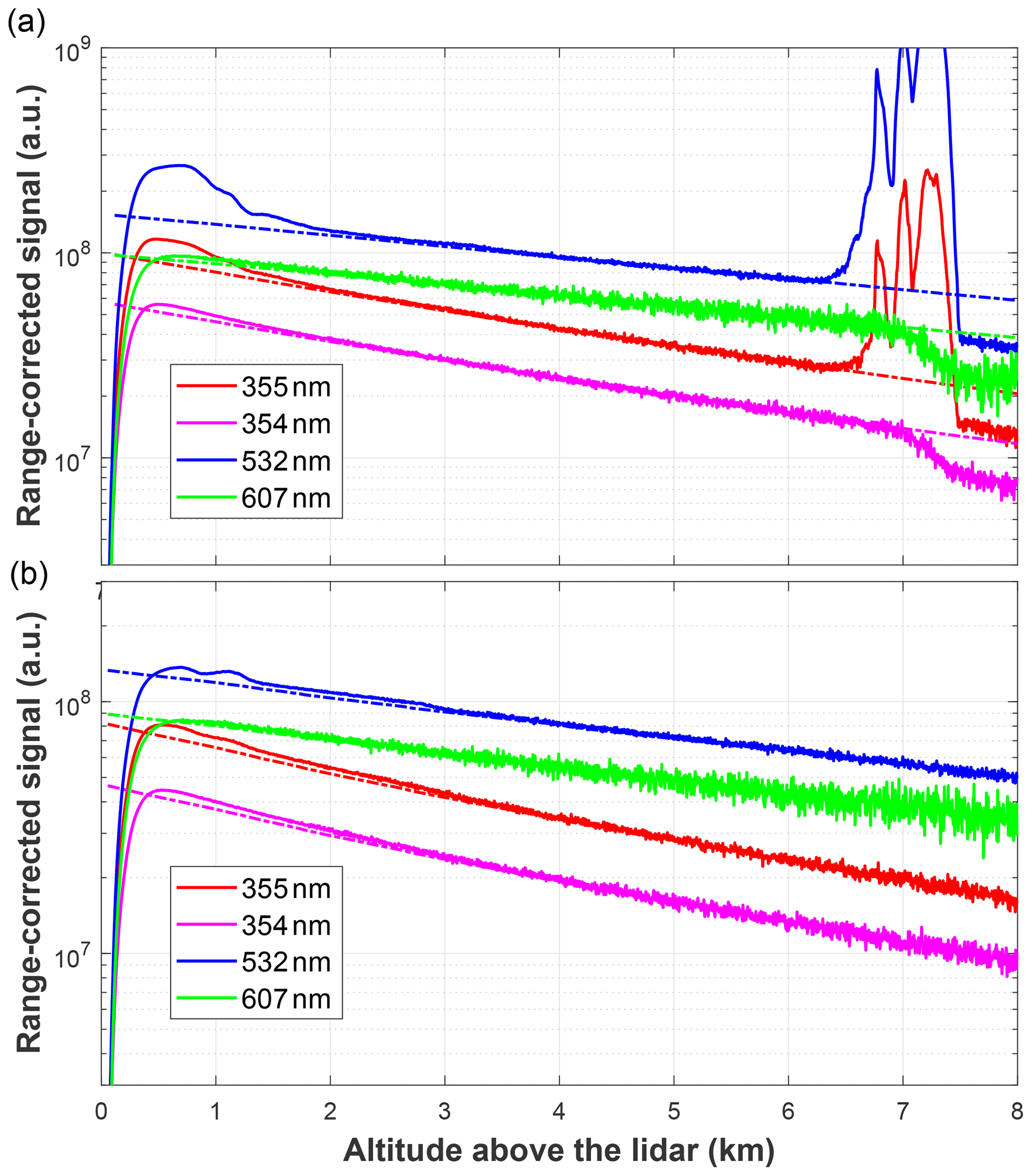
Figure 1 Range-corrected, Rayleigh-fitted lidar signals used in the example. The lidar signals (plotted with a solid line) were fitted to a Rayleigh profile (plotted with a dash-dotted line) obtained from the closest available radiosonde. (a) Signals from the 11 November 2021 measurement at 20:41 UTC, with radiosonde from 12 November 2021 at 00:00 UTC. (b) Signals from the 1 December 2021 measurement at 01:44 UTC, with radiosonde from 1 December 2021 at 00:00 UTC.

Figure 2 presents the backscatter coefficients obtained with the Raman method (Eq. 9; no smoothing applied to the signals) at 355 and 532 nm, neglecting the difference between the aerosol extinction coefficients at the emitted and Raman wavelengths. Note that this approximation is very well justified when the Raman channel is a purely rotational one, as in the case of the backscatter coefficient at 355 nm, since the two signals employed are at almost the same wavelength. Figure 2 shows that the aerosol backscatter coefficient at both wavelengths was much lower for the 1 December measurement than for the 11 November one. It also shows that the backscatter coefficient for the same day is higher at the shorter wavelength. Figure 2 also warns of a possible breakdown of the equal-overlap function hypothesis for the elastic and Raman channels, more clearly seen examining the profiles of 1 December: while the 532 nm aerosol backscatter coefficient shows a reasonable behavior until very low altitudes, the 355 nm one has a sudden fall below approximately 400 m. For this reason, in this particular case of optical alignment we should distrust the overlap function retrieval below that height for all cases.

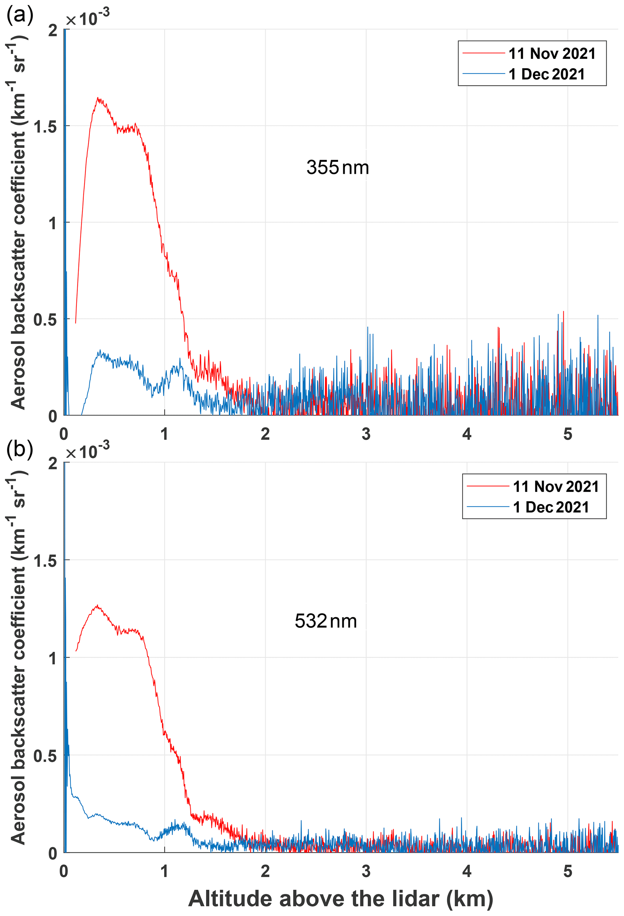
Figure 2 Aerosol backscatter coefficient using the Raman method formula. Upper graph: nominally at 355 nm using the 355 nm elastic channel and the 354 nm purely rotational channel. Lower graph: nominally at 532 nm using the 532 nm elastic channel and the 607 nm vibro-rotational Raman channel.

Figure 3 shows the results of the overlap function retrieval with our formulation (Eq. 15; neglecting the differential aerosol transmission terms $\exp \left\{{\int }_R^{R_{\mathrm{m}}}\left[{\mathit{\alpha }}_{\mathrm{a}\mathrm{0}}\right(x)-{\mathit{\alpha }}_{\mathrm{a}R}(x\left)\right]\mathrm{d}x\right\}$ assumed 1; see Appendix B for the assessment of the error bound entailed by this assumption) for three “reasonable” lidar ratios (25, 50 and 75 sr) from the 11 November 2021 measurement. The reference height is taken at 6 km, where the Rayleigh fit of the signals indicates the absence of aerosol (in agreement with the profiles of Figs. 1 and 2). The detected lidar signal sequences are noisy, especially the Raman ones, whereas the overlap function cannot have steep or sudden variations at far ranges; therefore, a smoothing procedure, coupled with a Monte Carlo routine to assess the residual error bars, has been employed. An overlap profile retrieved with the original noisy sequences (only for 50 sr lidar ratio) is plotted as well.

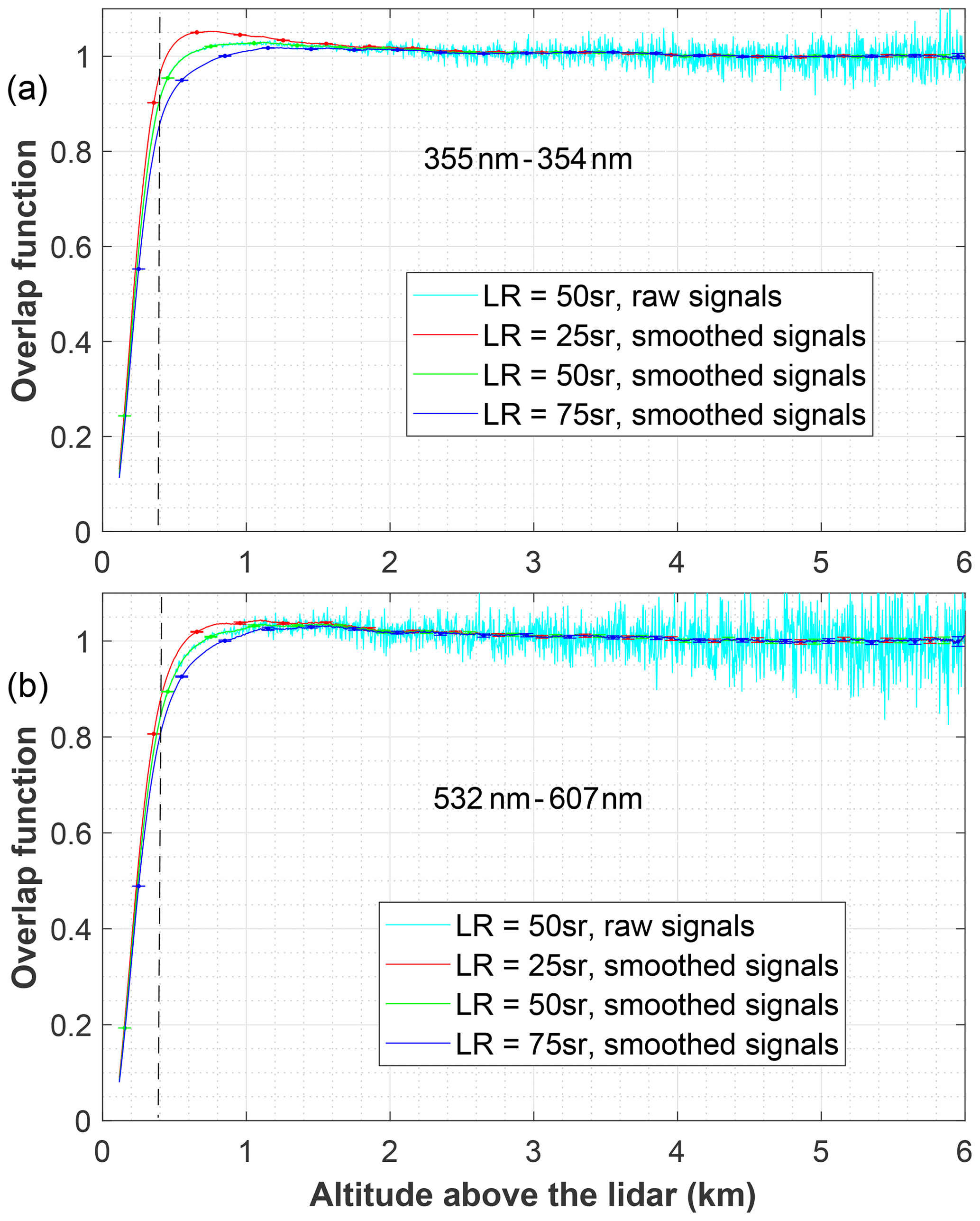
Figure 3 Overlap functions retrieved assuming different lidar ratios (LRs) at 355 nm (a) and 532 nm (b) from measurements carried out on 11 November 2021. A smoothing procedure described in the text has been applied, and error bars are shown. As a reminder of the applied smoothing, a raw result for a 50 sr lidar ratio is shown in light blue. The vertical discontinuous line marks the 400 m height below which the correction is to be mistrusted.

The raw elastic and Raman signal sequences detected by our lidar were fitted to a Rayleigh reference profile obtained from a nearby radiosonde. The sequences were corrected in range as well, being all the processes common in lidar inversion techniques. The result of this process leads to X(n) and X_R(n), standing for elastic and Raman signal sequences. Previous (noisy) estimates of the overlap profiles were calculated with these sequences.

These sequences were then smoothed to reduce the remaining noise, especially in the segments corresponding to high altitudes. This smoothing uses an adaptive sliding average approach. Each sample of the smoothed sequence was calculated as

$$\begin{array}{}\text{(19)}& X_{X\mathit{\_}\mathrm{sm}}\left(n\right)={\displaystyle \frac{\mathrm{1}}{L+\mathrm{1}}}\sum _{i=n-L/\mathrm{2}}^{n+L/\mathrm{2}}{X}_X\left(i\right),\end{array}$$

where the sub-index X stands for either elastic or Raman. The averaging window length L varies from 1 to 150 (3.75 to 562.5 m considering the raw range resolution of our lidar) as n grows. For low altitudes (low n) the noise is not significant, and the expected lidar signals show relevant variations, so L must be short, while it can be made longer for sequence segments corresponding to farther ranges, especially in the molecular zone.

The noise of these signals is estimated by comparing the non-smoothed sequences with the smoothed one. The estimation of this noise is necessary to create the different realizations in a Monte Carlo strategy to compute the error bars of the overlap estimation. Considering that the sequences have been smoothed by performing a (L+1)-long average, the standard deviation of the nth sample is estimated as (Papoulis and Pillai, 2002)

$$\begin{array}{}\text{(20)}& \mathrm{\Delta }{X}_X\left(n\right)={\displaystyle \frac{\mathrm{1}}{\sqrt{L+\mathrm{1}}}}\sqrt{{\displaystyle \frac{\mathrm{1}}{\mathrm{2}L+\mathrm{1}}}\sum _{i=n-L}^{n+L}\left[X_X\right(i)-X_{X\mathit{\_}\mathrm{sm}}(i){]}^{\mathrm{2}}}.\end{array}$$

The uncertainty of the calculated overlap profiles is estimated by using a common Monte Carlo approach. With the statistics obtained with Eqs. (19) and (20), N_MC (usually N_MC≈100) pairs of statistically independent elastic and Raman signal sequences are synthesized. Each of these synthesized sequences are generated as

$$\begin{array}{}\text{(21)}& X_{X\mathit{\_}k}\left(n\right)=X_{X\mathit{\_}\mathrm{sm}}\left(n\right)+e_{X\mathit{\_}k}\left(n\right),\end{array}$$

where each e_{X_k}(n) is a realization of a Gaussian random variable with 0 average and standard deviation ΔX_X(n).

With these N_MC sequence pairs, N_MC overlap profiles Ov_k(n) are calculated. The average overlap profiles Ov(n) and error bars ΔOv(n) presented in the next figures have been calculated as (Papoulis and Pillai, 2002)

$$\begin{array}{}\text{(22)}& \text{Ov}\left(n\right)={\displaystyle \frac{\mathrm{1}}{N_{\mathrm{MC}}}}\sum _{k=\mathrm{1}}^{\mathrm{100}}{\text{Ov}}_k\left(n\right),\end{array}$$

$$\begin{array}{}\text{(23)}& \mathrm{\Delta }\text{Ov}\left(n\right)=\sqrt{{\displaystyle \frac{\sum _{k=\mathrm{1}}^{N_{\mathrm{MC}}}\left[{\text{Ov}}_k\right(n)-\text{Ov}(n){]}^{\mathrm{2}}}{\left(N_{\mathrm{MC}}-\mathrm{1}\right)}}}.\end{array}$$

In Fig. 4 the retrieved overlap functions from data of 1 December 2021 are represented for the same assumed lidar ratios as in Fig. 3. Because we have arbitrarily normalized the profile to the reference height, where the overlap function has reached a stable value, values greater than 1, as shown in Figs. 2 and 3, at lower ranges are possible and reveal a non-perfect alignment, in particular, a slight crossing between the laser beam and the receiver field-of-view axes, leading to a loss of energy from the far range (see for example Fig. 1a in Kokkalis, 2017, with laser tilt A_tilt, half-width laser beam divergence (LBD) and receiver field of view (RFOV) fulfilling the conditions $A_{\mathrm{tilt}}+\text{LBD}>\text{RFOV}$ and $A_{\mathrm{tilt}}-\text{LBD}<\text{RFOV}$). As expected (Sect. 3), being the aerosol backscatter coefficients at both wavelengths lower in this measurement, the difference between the overlaps obtained with different lidar ratios is lower than for 11 November. Also, because the backscatter coefficient at 532 nm is lower than at 355 nm, the differences in the retrieved overlap functions are less sensitive to the guessed lidar ratio at the former wavelength, being in fact almost negligible. An overlap profile retrieved with the original noisy sequences (for LR =50 sr) is plotted as well. Although using a different, explicit non-iterative formulation, the method presented in this paper relies on the same basis as the one given by Ulla Wandinger and Albert Ansmann. The reader can check that for the same measured data and assumed lidar ratio both methods for a sufficient number of iterations in Wandinger and Ansmann (2002) yield indistinguishable results.

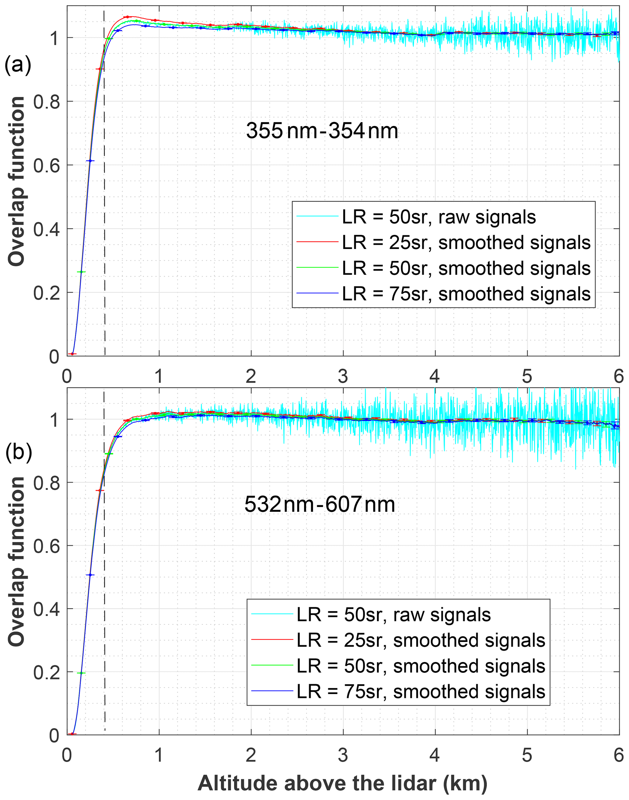
Figure 4 Overlap functions retrieved assuming different lidar ratios (LRs) at 355 nm (a) and 532 nm (b) from measurements carried out on 1 December 2021. The same smoothing procedure and method to obtain error bars as in Fig. 2 have been employed. As in Fig. 2, the vertical dashed line marks the range below which the retrieval is subject to caution. As a reminder of the applied smoothing, a raw result for a 50 sr lidar ratio is shown in light blue.

5 Conclusions

Based on the same principle as in Wandinger and Ansmann (2002), i.e., that the aerosol backscatter coefficient derived by the Raman method (Ansmann et al., 1992) is not affected by the lidar range-varying overlap (under the assumption of the same overlap function for the elastic and the Raman channels), a new formulation for deriving the overlap function of an aerosol lidar system equipped with Raman channels has been presented. As input data, the method uses the elastic and Raman signals and a guess of the lidar ratio corresponding to the emitted wavelength of interest. The novelty of our approach consists of the derivation of an explicit formula in which no iterations have to be performed.

Results of the formula are illustrated with two examples, both with a low aerosol load but one of them with a much lower load than the other, showing the effect of the guessed lidar ratio on the overlap function retrievals.

The explicit formula allows one to assess the errors committed when an erroneous lidar ratio is used (Sect. 3), showing, as already stated by Wandinger and Ansmann (2002), that the retrieval of the overlap function is less prone to errors when performed in clear atmospheres. It also makes it possible to find systematic error bounds associated with the uncertainty in the different aerosol transmissions at the elastic and the Raman wavelengths when Raman vibro-rotational channels are used (Appendix B). Section 3 also cautions against trying to derive a lidar ratio using the corrected-for-overlap signal. Actually, one could be tempted to think of the following procedure: an overlap function is retrieved using a guessed aerosol lidar ratio; with that overlap function, the Raman signal is corrected, and an aerosol extinction coefficient is calculated, which, divided by the aerosol backscatter, gives a new lidar ratio, which is in turn used to retrieve a new overlap function, and so on. However, Eq. (18) shows that this procedure does not converge, for if a too low lidar ratio is used as the first guess, the overlap function will be enhanced in the range with aerosol; when correcting with this enhanced overlap function, the Raman signal will be suppressed, which will give rise to an aerosol extinction coefficient lower than due and, consequently, to a lower new lidar ratio. A similar reasoning goes on if the guessed aerosol lidar ratio is too high. The determination of the required lidar ratio from Raman inversions needs atmospheric regions with both significant aerosol load and stable overlap. However, in cases with regions where both conditions are fulfilled, using the retrieved lidar ratio for overlap estimations requires assuming that the type of aerosol is uniform down to the ground. Moreover, as seen in Sect. 3, in aerosol-loaded scenarios, errors in the lidar ratio determination yield greater errors in the estimation of the overlap profile. A more conservative approach is to stay with situations with a low aerosol load at low altitudes and use the aerosol backscatter profiles derived with the Raman method (e.g., Fig. 2) together with a sun- or lunar-photometer aerosol optical depth (AOD) measurement and find the aerosol lidar ratio that, multiplied by the integrated aerosol backscatter coefficient, would yield the AOD measured by the photometer. However, these techniques are out of the scope of this paper, which aims only at presenting the explicit formulation of the overlap function and discussing the effect of the assumed lidar ratio on the retrieved profiles.

Appendix A: Derivation of the explicit form of the overlap function

We outline here the mathematical details to obtain Eq. (15). Using the definitions of Eqs. (12), (13) and (14), Eq. (10) can be written as the Volterra integral equation

$$\begin{array}{}\text{(A1)}& f\left(R\right)=g\left(R\right)+\mathit{\varphi }\left(R\right){\int }_R^{R_{\mathrm{m}}}f\left(x\right)\mathit{\psi }\left(x\right)\mathrm{d}x,\end{array}$$

which is amenable to a differential equation. In order to do that, we define the function

$$\begin{array}{}\text{(A2)}& u\left(R\right)={\int }_R^{R_{\mathrm{m}}}f\left(x\right)\mathit{\psi }\left(x\right)\mathrm{d}x,\end{array}$$

which, substituting into Eq. (A1), yields

$$\begin{array}{}\text{(A3)}& f\left(R\right)=g\left(R\right)+u\left(R\right)\mathit{\varphi }\left(R\right).\end{array}$$

We next take the derivative Eq. (A2)

$$\begin{array}{}\text{(A4)}& {\displaystyle \frac{\mathrm{d}}{\mathrm{d}R}}u\left(R\right)=-f\left(R\right)\mathit{\psi }\left(R\right)\end{array}$$

and substitute Eq. (A3) on it to obtain, after reordering terms,

$$\begin{array}{}\text{(A5)}& {\displaystyle \frac{\mathrm{d}}{\mathrm{dR}}}u\left(R\right)+\mathit{\varphi }\left(R\right)\mathit{\psi }\left(R\right)u\left(R\right)=-g\left(R\right)\mathit{\psi }\left(R\right).\end{array}$$

To integrate that equation, we define an integrating factor $\exp \left[{\int }_R^{R_{\mathrm{m}}}\mathit{\varphi }\right(x\left)\mathit{\psi }\right(x\left)\mathrm{d}x\right]$ and multiply both members of Eq. (A5) by it, which allows us to recast the equation as

$$\begin{array}{}\text{(A6)}& \begin{array}{rl}{\displaystyle \frac{\mathrm{d}}{\mathrm{d}R}}& \left\{u\left(R\right)\exp \left[{\int }_R^{R_{\mathrm{m}}}\mathit{\varphi }\left(x\right)\mathit{\psi }\left(x\right)\mathrm{d}x\right]\right\}\\ & =-g\left(R\right)\mathit{\psi }\left(R\right)\exp \left[{\int }_R^{R_{\mathrm{m}}}\mathit{\varphi }\left(x\right)\mathit{\psi }\left(x\right)\mathrm{d}x\right].\end{array}\end{array}$$

Integrating both members of Eq. (A6) between R and R_m and noting that, by construction, u(R_m)=0, leads to

$$\begin{array}{}\text{(A7)}& \begin{array}{rl}u\left(R\right)& =\exp \left[{\int }_R^{R_{\mathrm{m}}}\mathit{\varphi }\left(x\right)\mathit{\psi }\left(x\right)\mathrm{d}x\right]{\int }_R^{R_{\mathrm{m}}}g\left(x\right)\mathit{\psi }\left(x\right)\\ & \exp \left[-{\int }_x^{R_{\mathrm{m}}}\mathit{\varphi }\left(x^{\prime }\right)\mathit{\psi }\left(x^{\prime }\right)\mathrm{d}{x}^{\prime }\right]\mathrm{d}x.\end{array}\end{array}$$

Finally, taking the derivatives of both members of Eq. (A7) and considering Eq. (A4) one obtains

$$\begin{array}{}\text{(A8)}& \begin{array}{rl}f\left(R\right)& =g\left(R\right)+\mathit{\varphi }\left(R\right)\exp \left[{\int }_R^{R_{\mathrm{m}}}\mathit{\varphi }\left(x\right)\mathit{\psi }\left(x\right)\mathrm{d}x\right]\\ & \underset{R}{\overset{R_{\mathrm{m}}}{\int }}g\left(x\right)\mathit{\psi }\left(x\right)\exp \left[-{\int }_x^{R_{\mathrm{m}}}\mathit{\varphi }\left(x^{\prime }\right)\mathit{\psi }\left(x^{\prime }\right)\mathrm{d}{x}^{\prime }\right]\mathrm{d}x.\end{array}\end{array}$$

In our case, $g\left(R\right)=\frac{\mathrm{1}}{\mathrm{2}}\frac{X\left(R_{\mathrm{m}}\right)}{{\mathit{\beta }}_{\mathrm{m}\mathrm{0}}\left(R_{\mathrm{m}}\right)}\mathit{\varphi }\left(R\right)$ (see Eqs. 12 and 13), which makes

$$\begin{array}{}\text{(A9)}& O\left(R\right)={\displaystyle \frac{\mathrm{1}}{f\left(R\right)}}={\displaystyle \frac{\mathrm{2}{\mathit{\beta }}_{\mathrm{m}\mathrm{0}}\left(R_{\mathrm{m}}\right)}{X\left(R_{\mathrm{m}}\right)\mathit{\varphi }\left(R\right)\exp \left[{\int }_R^{R_{\mathrm{m}}}\mathit{\varphi }\right(x\left)\mathit{\psi }\right(x\left)\mathrm{d}x\right]}}.\end{array}$$

Appendix B: Systematic error bounds

We assess the error incurred in the estimation of O(R) (Eq. 15) when neglecting the difference in molecular lidar ratios and the differential aerosol transmission term.

We start by noting that (Bucholtz, 1995; D'Amico et al., 2016) the molecular lidar ratio at a wavelength λ can be written as

$$\begin{array}{}\text{(B1)}& S_{\mathrm{m}\mathit{\lambda }}=S_{\mathrm{m}}\left(\mathrm{1}+{\displaystyle \frac{{\mathit{\delta }}_{n\mathit{\lambda }}}{\mathrm{2}}}\right),\end{array}$$

with $S_{\mathrm{m}}=\frac{\mathrm{8}\mathit{\pi }}{\mathrm{3}}$, and δ_nλ is the depolarization factor that takes into account the anisotropy of the air molecules (Bucholtz, 1995). We can then write the terms S_m0β_m0(x)−S_mRβ_mR(x) in Eq. (15) as

$$\begin{array}{}\text{(B2)}& \begin{array}{rl}{S}_{\mathrm{m}\mathrm{0}}{\mathit{\beta }}_{\mathrm{m}\mathrm{0}}\left(x\right)& -S_{\mathrm{m}R}{\mathit{\beta }}_{\mathrm{m}R}\left(x\right)=S_{\mathrm{m}}\left[{\mathit{\beta }}_{\mathrm{m}\mathrm{0}}\right(x)-{\mathit{\beta }}_{\mathrm{m}R}(x\left)\right]\\ & +{\displaystyle \frac{S_{\mathrm{m}}}{\mathrm{2}}}\left[{\mathit{\delta }}_{n\mathrm{0}}{\mathit{\beta }}_{\mathrm{m}\mathrm{0}}\right(x)-{\mathit{\delta }}_{nR}{\mathit{\beta }}_{\mathrm{m}R}(x\left)\right],\end{array}\end{array}$$

where, for a vibro-rotational Raman channel, $\frac{S_{\mathrm{m}}}{\mathrm{2}}\left[{\mathit{\delta }}_{n\mathrm{0}}{\mathit{\beta }}_{\mathrm{m}\mathrm{0}}\right(x)-{\mathit{\delta }}_{nR}{\mathit{\beta }}_{\mathrm{m}R}(x\left)\right]>\mathrm{0}$.

The terms α_a0(x)−α_aR(x) can be written as

$$\begin{array}{}\text{(B3)}& {\mathit{\alpha }}_{\mathrm{a}\mathrm{0}}\left(x\right)-{\mathit{\alpha }}_{\mathrm{a}R}\left(x\right)=\left[\mathrm{1}-{\left({\displaystyle \frac{{\mathit{\lambda }}_{\mathrm{0}}}{{\mathit{\lambda }}_R}}\right)}^{a\left(x\right)}\right]{\mathit{\alpha }}_{\mathrm{a}\mathrm{0}}\left(x\right),\end{array}$$

with a(x) being the Ångström exponent, which is in general positive.

By examining Eqs. (15), (B2) and (B3), it is seen that

$$\begin{array}{}\text{(B4)}& O\left(R\right)>O_{\mathrm{0}}\left(R\right),\end{array}$$

with O₀(R) defined as

$$\begin{array}{}\text{(B5)}& \begin{array}{rl}{O}_{\mathrm{0}}\left(R\right)& ={\displaystyle \frac{{\mathit{\beta }}_{\mathrm{m}\mathrm{0}}\left(R_{\mathrm{m}}\right)X_R\left(R\right)}{{\mathit{\beta }}_{\mathrm{m}\mathrm{0}}\left(R\right)X_R\left(R_{\mathrm{m}}\right)}}\\ & \exp \left\{\mathrm{2}{\int }_R^{R_{\mathrm{m}}}\left[S_{\mathrm{a}\mathrm{0}}\right(x)-S_{\mathrm{m}\mathrm{0}}]{\mathit{\beta }}_{\mathrm{m}\mathrm{0}}\left(x\right)\mathrm{d}x\right\}\\ & \exp \left\{S_{\mathrm{m}}{\int }_R^{R_{\mathrm{m}}}\left[{\mathit{\beta }}_{\mathrm{m}\mathrm{0}}\right(x)-{\mathit{\beta }}_{\mathrm{m}R}(x\left)\right]\mathrm{d}x\right\}\\ & \exp \mathit{\{}\mathrm{2}{\displaystyle \frac{X_R\left(R_{\mathrm{m}}\right)}{X_{\mathrm{m}}}}{\int }_R^{R_{\mathrm{m}}}{\displaystyle \frac{S_{\mathrm{a}\mathrm{0}}\left(x\right){\mathit{\beta }}_{\mathrm{m}\mathrm{0}}\left(x\right)X\left(x\right)}{X_R\left(x\right)}}\\ & \exp \left(-S_{\mathrm{m}}{\int }_x^{R_{\mathrm{m}}}[{\mathit{\beta }}_{\mathrm{m}\mathrm{0}}\left(x^{\prime }\right)-{\mathit{\beta }}_{\mathrm{m}R}\left(x^{\prime }\right)]\mathrm{d}{x}^{\prime }\right)\mathrm{d}x\mathit{\}},\end{array}\end{array}$$

i.e., ignoring the difference in the aerosol transmissions at the elastic and Raman wavelengths and

$$\begin{array}{}\text{(B6)}& \begin{array}{rl}& O\left(R\right)<O_{\mathrm{0}}\left(R\right)\\ & \times \exp \mathit{\left\{}{\displaystyle \frac{S_{\mathrm{m}}}{\mathrm{2}}}{\int }_R^{R_{\mathrm{m}}}\right[{\mathit{\delta }}_{n\mathrm{0}}{\mathit{\beta }}_{\mathrm{m}\mathrm{0}}\left(x\right)-{\mathit{\delta }}_{nR}{\mathit{\beta }}_{\mathrm{m}R}\left(x\right)\left]\mathrm{d}x\mathit{\right\}}\\ & \exp \mathit{\left\{}\right[\mathrm{1}-{\left({\displaystyle \frac{{\mathit{\lambda }}_{\mathrm{0}}}{{\mathit{\lambda }}_R}}\right)}^{a_{max}}\left]{\text{AOD}}_{\mathrm{0}}\mathit{\right\}}\\ & \exp \mathit{\{}-\mathit{\{}\mathrm{2}{\displaystyle \frac{X_R\left(R_{\mathrm{m}}\right)}{X_{\mathrm{m}}}}{\int }_R^{R_{\mathrm{m}}}{\displaystyle \frac{S_{\mathrm{a}\mathrm{0}}\left(x\right){\mathit{\beta }}_{\mathrm{m}\mathrm{0}}\left(x\right)X\left(x\right)}{X_R\left(x\right)}}\\ & \exp (-S_{\mathrm{m}}{\int }_x^{R_{\mathrm{m}}}[{\mathit{\beta }}_{\mathrm{m}\mathrm{0}}\left(x^{\prime }\right)-{\mathit{\beta }}_{\mathrm{m}R}\left(x^{\prime }\right)\left]\mathrm{d}{x}^{\prime }\right)\\ & \mathrm{d}x{\mathit{\}}}^{\exp \left\{-\frac{S_{\mathrm{m}}}{\mathrm{2}}{\int }_R^{R_{\mathrm{m}}}\left[{\mathit{\delta }}_{n\mathrm{0}}{\mathit{\beta }}_{\mathrm{m}\mathrm{0}}\right(x)-{\mathit{\delta }}_{nR}{\mathit{\beta }}_{\mathrm{m}R}(x\left)\right]\mathrm{d}x\right\}\exp \left\{-[\mathrm{1}-{\left(\frac{{\mathit{\lambda }}_{\mathrm{0}}}{{\mathit{\lambda }}_R}\right)}^{a_{max}}]{\text{AOD}}_{\mathrm{0}}\right\}-\mathrm{1}}\mathit{\}},\end{array}\end{array}$$

with AOD₀ being the aerosol optical depth at the wavelength λ₀ and a_max the maximum Ångström exponent found along the lidar line of sight.

As an example, the upper-bound factor $O\left(R\right)/O_{\mathrm{0}}\left(R\right)$ according to Eq. (B6), with the data used to obtain the lower panel of Fig. 3 and S_a=50 sr, AOD₀=0.05 and $a_{max}=\mathrm{1.3}$, is given in Fig. B1. We see as well that considering $S_{\mathrm{m}\mathrm{0}}=S_{\mathrm{m}R}=S_{\mathrm{m}}$ has only a small impact on the bound.

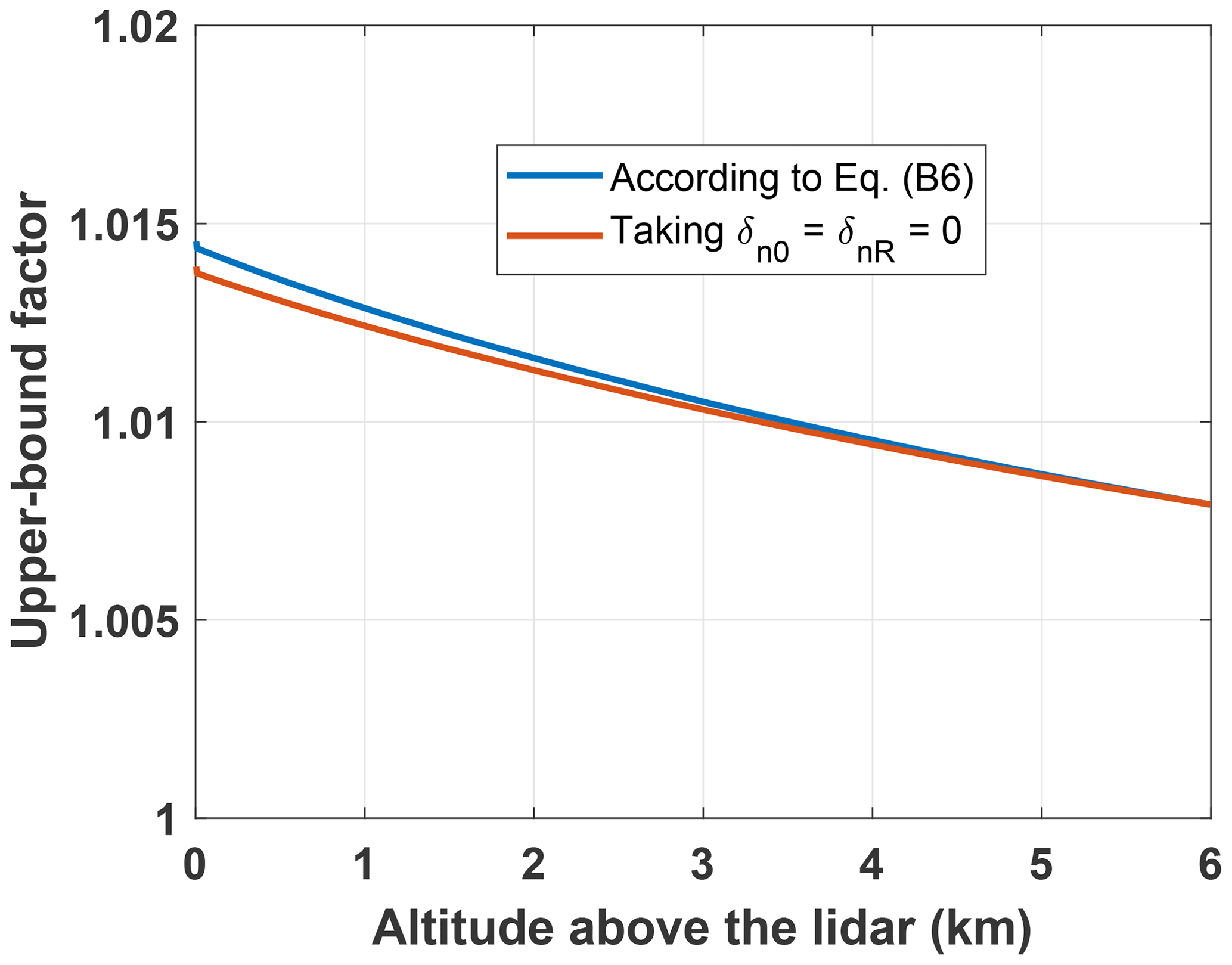
Figure B1 Upper-bound factor of the overlap function obtained with the wavelength combination 532–607 nm for the measurement of 1 December 2021, assuming a 50 sr aerosol lidar ratio, a 0.05 aerosol optical depth and a 1.3 maximum Ångström exponent.