Analysis of 2D airglow imager data with respect to dynamics using machine learning

We demonstrate how machine learning can be easily applied to support the analysis of large quantities of excited hydroxyl (OH^*) airglow imager data. We use a TCN (temporal convolutional network) classification algorithm to automatically pre-sort images into the three categories “dynamic” (images where small-scale motions like turbulence are likely to be found), “calm” (clear-sky images with weak airglow variations) and “cloudy” (cloudy images where no airglow analyses can be performed). The proposed approach is demonstrated using image data of FAIM 3 (Fast Airglow IMager), acquired at Oberpfaffenhofen, Germany, between 11 June 2019 and 25 February 2020, achieving a mean average precision of 0.82 in image classification. The attached video sequence demonstrates the classification abilities of the learned TCN.

Within the dynamic category, we find a subset of 13 episodes of image series showing turbulence. As FAIM 3 exhibits a high spatial (23 m per pixel) and temporal (2.8 s per image) resolution, turbulence parameters can be derived to estimate the energy diffusion rate. Similarly to the results the authors found for another FAIM station (Sedlak et al., 2021), the values of the energy dissipation rate range from 0.03 to 3.18 W kg⁻¹.

1 Introduction

Airglow imagers are a well-established method for studying UMLT (upper mesosphere–lower thermosphere) dynamics. As the shortwave infrared (SWIR) radiation of excited hydroxyl (OH^*) between approx. 82 and 90 km height (von Savigny, 2015; Wüst et al., 2017, 2020) is known to be the brightest diffuse emission during the nighttime (Leinert et al., 1998; Rousselot et al., 1999), atmospheric dynamics is observed using airborne (Wüst et al., 2019) or ground-based SWIR cameras (Taylor, 1997; Nakamura et al., 1999; Hecht et al., 2014; Pautet et al., 2014; Hannawald, 2016, 2019; Sedlak et al., 2016, 2021). OH^* measurements are also possible from satellites, where they can be made in limb- or nadir-viewing geometry (see Table 1 of Wüst et al., 2023, for limb instruments). The limb measurements address mainly the SWIR range and are mostly used for deriving information about the OH^* layer height and thickness. Nadir-looking instruments, however, such as VIIRS DNB (Day/Night Band nightglow imagery from the Visible Infrared Imaging Radiometer Suite) on board Suomi NPP (Suomi National Polar-orbiting Partnership) and JPSS-1 (Joint Polar Satellite System 1), which have been used for analyses of atmospheric dynamics until now, measure in the VIS (visible) range. In contrast to imager systems using an all-sky lens, which enable us to observe the entire dynamical situation of the nocturnal sky, operating an imager with a lens of long focal length and narrow aperture angles provides the opportunity to observe small-scale dynamical features in the UMLT with a high spatial resolution. This includes not only instability features of gravity waves, such as “ripples” (Peterson, 1979; Taylor and Hapgood, 1990; Li et al., 2017), but also turbulence (Hecht et al., 2021; Sedlak et al., 2016, 2021). Previous studies at Oberpfaffenhofen (Sedlak et al., 2016) and Otlica, Slovenia (Sedlak et al., 2021), using the high-resolution airglow imager FAIM 3 (Fast Airglow IMager) have shown that the observation of turbulent episodes in the OH^* layer is possible with this kind of instrument.

Turbulence marks the end of the life cycle of breaking gravity waves (Hocking, 1985). Having become dynamically or convectively unstable, the wave can no longer propagate and eventually breaks down developing eddies. Within this inertial subrange of turbulence, energy is cascaded to smaller and smaller structures until it is dissipated via viscous damping, causing a heating effect on the atmosphere. Observing turbulence episodes with high-resolution airglow imagers, the respective energy dissipation rate can be derived from the image series by reading out the typical length scale L of the eddies and the root-mean-square velocity U, i.e., the velocity of single eddy patches relative to the background motion (Hecht et al., 2021; Sedlak et al., 2021).

The energy dissipation rate ϵ is given by

$$\begin{array}{}\text{(1)}& \mathit{ϵ}=C_{\mathit{ϵ}}{\displaystyle \frac{U^{\mathrm{3}}}{L}}\end{array}$$

(Chau et al., 2020), where C_ϵ≈1 (Gargett, 1999). The results in Sedlak et al. (2021) suggest that, locally and within a few minutes, the heating rate driven by the turbulent breakdown of gravity waves can be as large as the daily chemical heating rates in the mesopause region (Marsh, 2011). Thus, one has to assume that this dynamically driven effect is of great importance for the energy budget of the atmosphere and needs to be included realistically in modern climate models.

In order to derive statistically reliable and also global information about gravity wave energy deposition in the UMLT, more and more high-resolution airglow imagers need to be deployed at different locations around the world. The largest challenge is to identify turbulence episodes in a rapidly growing data set of airglow images. While in former studies turbulence episodes were found by manual inspection (Sedlak et al., 2016, 2021), this will not be feasible anymore with much larger quantities of data.

When it comes to image recognition, artificial intelligence (AI) is a field that has seen tremendous progress in recent years (Fujiyoshi et al., 2019; Horak and Sablatnig, 2019; Guo et al., 2022). In particular, algorithms using neural networks (NNs) show a very good performance in identifying different objects in images and also have a quite efficient computation time. Using these methods to detect turbulence in airglow images presents several challenges that complicate the use of off-the-shelf image recognition algorithms:

• Turbulent movement manifests itself in a wide variety of shapes and structures.

• Structures in the OH^* layer appear blurred, and contrasts are strongly dominated by clouds.

• Turbulence can often only be identified in the dynamic course of a video sequence; single images of a turbulent episode are easily confused with clouds.

• The number of images showing turbulence is much smaller than the number of images showing no turbulence; thus there is an essential imbalance of available training data for the different categories.

All these aspects have the consequence that a direct extraction of turbulent episodes from the entire measurement data set is very difficult. However, some existing approaches exhibit promising advantages that could help in finding turbulence episodes. In this work, we show how NN-based methods can be combined into an algorithm that is easy to use and performs well in strongly reducing the database where turbulence can likely be found. We demonstrate the application and performance of this practical approach on OH^* airglow image data of the FAIM 3 instrument acquired at Oberpfaffenhofen, Germany, between 11 June 2019 and 25 February 2020.

Our goal is to explain our approach in a way that it is relatively easy to apply for airglow scientists who do not specialize in AI. Therefore, the description of the classification algorithm (Sect. 3) is in more detail than for example the introduction of the airglow instrument or the data preparation (Sect. 2).

2 Instrumentation and data preparation

The OH^* airglow imager FAIM 3 is based on the short-wave infrared (SWIR) camera Cheetah CL by Xenics nv. The system has already been described in Sedlak et al. (2016); therefore, only the most important information is given here.

The SWIR camera consists of a 512 × 640 pixels InGaAs focal plane array, which is sensitive to infrared radiation with a wavelength between 0.9 and 1.7 µm. Images are acquired automatically during each night (solar zenith angle > 100^∘) with a temporal resolution of 2.8 s. Since June 2019 measurements have been performed at the German Aerospace Center (DLR) site at Oberpfaffenhofen (48.09^∘ N, 11.28^∘ E), Germany, with a zenith angle of 34^∘ and an azimuthal angle of 204^∘ (SSW direction). Due to the aperture angles of 5.9 and 7.3^∘, this results in a trapezium-shaped field of view (FOV) in the mean OH^* emission height at ca. 87 km with size 175 km² (13.0–13.9 km × 13.1 km) and a mean spatial resolution of 23 m per pixel. The FOV is located ca. 80 km south of Augsburg, Germany.

The database used in this work consists of nocturnal image series acquired between 11 June 2019 and 25 February 2020. During this period, measurements were performed during 258 nights. Analyzing keograms, 95 (37 %) of these nights show complete cloud coverage and prevent analyses based on airglow observations. The remaining 163 nights exhibit a clear sky either all of the time or at least temporarily (at least ca. 30 min), so the OH^* layer is visible in a total of 188 episodes (it is possible that a single night may have several clear episodes interspersed with cloudy episodes).

The images are prepared for analysis by performing a flat-field correction and transforming each of them onto an equidistant grid (for further details see Hannawald et al., 2016). In order to completely remove any pattern remnants, such as reflections of the objective lens in the window, the average image of each episode (a pixel-wise mean of all images in that episode) is subtracted from the individual images.

3 Image classification with neural networks

3.1 Label classes

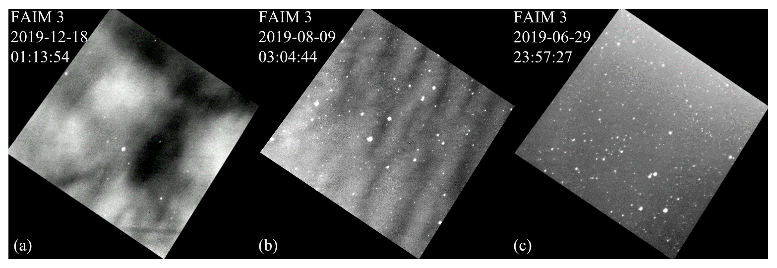
When looking at the temporal course of the image data, three main types of observation can be distinguished, which we use as label classes for the classification algorithm (typical examples of these label classes are shown in Fig. 1):

Figure 1 Typical examples of the three label classes: (a) cloudy, (b) dynamic and (c) calm.

• Cloudy. These are episodes of clouds or cloud fragments moving through the image (Fig. 1a). These cloudy episodes are too short or too faint to be recognized during keogram analysis (see Sect. 2). The image series are characterized by sharp contrasts and fast movement of coherent structures (compared with structures in the “dynamic” class). Often (but not necessarily) stars are covered by the clouds.

• Dynamic. These are cloud-free episodes with pronounced moving OH^* airglow structures (Fig. 1b), including waves and eddies. OH^* dynamics can be distinguished from cloud movement due to slower velocities, blurrier edges and (except for extended wave fields) more isotropic movements.

• Calm. These are cloud-free episodes with weak movement in the OH^* layer (Fig. 1c). The images appear quite homogeneous and hardly change in the temporal course.

The goal of the classification algorithm is to automatically and reliably identify the dynamic label class. In a subsequent step, which is not part of this work, these episodes can then be analyzed with respect to turbulence.

3.2 Image features

We calculated a set of 1-dimensional features for each image series that we believe help to distinguish the categories introduced in Sect. 3.1.

The mean value and standard deviation are calculated for every image. The mean value feature is calculated based on the assumption that “cloudy” episodes have a higher intensity than “calm” episodes due to reflections from ground lights or the moon. The standard deviation of the label class calm is expected to be lower, whereas the label class cloudy is expected to have higher values, since clouds exhibit both very bright areas (strongly reflecting clouds) and very dark areas (shades or small clear-sky gaps in the cloud coverage). Both the mean and the standard deviation of the label class cloudy are expected to have intermediate values between those of the calm and cloudy classes. We refer to these two features (mean value and standard deviation) as the basic features.

They are supplemented by three texture-based features derived from the grey level co-occurrence matrix (GLCM) as described in Zubair and Alo (2019). Homogeneity is the first of these three texture-based features and is a method of measuring the similarity of neighboring pixels in an image. If its value is particularly high, it suggests a high similarity of adjacent pixels (Zhou et al., 2017). This may indicate a positive correlation with the label class calm. The second texture-based feature, dissimilarity, is inversely correlated to homogeneity and thus could help to identify the episodes containing a lot of motion. The third texture-based feature, uniformity, is particularly high if the image has uniform structures. On the other hand, this value is very small as soon as the image contains heterogeneous structures.

Additionally, features which are based on a 2-dimensional fast Fourier transform (2D-FFT) as described in Hannawald et al. (2019) are derived for each image. They are called the “PSD” feature group in the following. As in Sedlak et al. (2021), the 2D-FFT is applied to a squared cutout centered at the image center with side length 406 pixels (9.3 km). This results in 2-dimensional spectra, which depend on the zonal and the meridional wavenumber. They are integrated over these wavenumbers such that the power spectral density (PSD) as a function of horizontal wavenumber k is derived. According to Kolmogorov (1991), the log(PSD)–log(k) shows different slopes, which depend on whether the observed field is in the buoyancy (dominating energy transport by waves), the inertial (energy cascades to smaller scales) or the viscous subrange (viscous damping of movements). Therefore, the feature slope is derived as the linear fit in the log(PSD)–log(k) plot. Then, the PSD is integrated over all k and the change in this value per time step is calculated. This feature is called DiffIPSD (differences in integrated PSD) and takes into account the fact that clouds tend to cause stronger fluctuations over time than during clear-sky episodes. Last, the PSD is integrated over all k and over the whole night. This feature is denoted IPSD (integrated PSD).

In total, we calculate eight different features for each image. They are summarized again in Table 1 for a better overview.

Table 1 Image features used with the classification algorithm.

3.3 Data basis for the classification algorithm

The features introduced in the last subsection were calculated for every fifth image. This results in a temporal resolution of 14 s and data set of approximately 240 000 time steps. About 105 000 time steps are assigned to the label class calm, 65 000 to cloudy and 70 000 to dynamic. This data set is divided into three parts: training, validation and test data. The partition is performed as follows: first, the list of all measured nights is arranged chronologically and divided into parts with 10 measured nights each. From these parts, one measured night is randomly selected and assigned to the test data. From the remaining nine measured nights, two are randomly assigned to the validation data. The remaining seven measured nights are assigned to the training data. This results in approximately 70 % training data, 20 % validation data and 10 % test data by looking at the total number of time steps. All features of the three data sets were independently normalized to the range 0 to 1. Before normalization, the outliers (lowest and highest 0.05 quantile) were replaced by the highest value of the lowest 0.05 quantile and the lowest value of the highest 0.05 quantile respectively.

The training data set is used to train a neural network, and at the end of an epoch (one training cycle of the whole training data set), the result and the learning progress are checked using the validation data set. After running through all 100 epochs and additional possible manual adjustments to the classification procedure, the final quality of a classifier is determined on the test data set. This procedure serves, among other things, to avoid overfitting to the training data set. In order to use this procedure properly, the training, validation and test data must be different from each other. In our case, this is ensured by dividing the complete data set into training, validation and test data set by complete nights and not by individual parts of a night. Features from one night may be more similar to each other than features from different nights, which could lead to inadvertent overfitting if parts of a night were used for the partitioning into the training, validation and test data set.

3.4 Classification algorithm

A neural network consists of an input and an output layer as well as one or more hidden layers in between (in the latter case, the network is called “deep”). Each layer is composed of one or more neurons, which work like biological neurons: multiple input signals are passed to a neuron. If the aggregated inputs exceed a certain strength, the neuron is activated and transmits a signal to its outputs. For artificial neurons, we assume that the incoming signal (for all but the input layer) is the weighted sum from other neurons' outputs plus a bias. The activation of the artificial neuron happens according to an activation function (e.g., rectified linear unit, ReLU, as described in Nair and Hinton, 2010). The different hidden layers are used to learn the true output. This is done by optimizing the weights and the bias for each neuron.

The goal of our neural network is to assign a FAIM image to one of the three label classes calm, cloudy or dynamic. Hence, the output layer of our NN has three neurons. Each output neuron represents a label class and is supposed to output the probability of the respective class given the input features. These three output probabilities are combined in a vector, the prediction vector.

Since considering a sequence of images instead of an individual image often simplifies the discrimination between the different classes, our neural network uses sequences as input. In our case these are sequences of the abovementioned features and not sequences of images. The sequences of features are derived from several consecutive images that are located symmetrically in time around the original image that is to be classified.

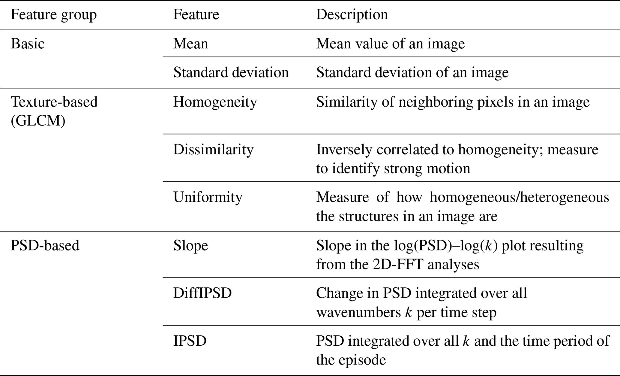
In order to attribute one image to a specific class, we used a temporal convolutional network (TCN; see, e.g., Bai et al., 2018) in the TensorFlow Keras implementation of Rémy (2020). TCNs are based on dilated convolutions, so at each neuron of the hidden layer, a convolution takes place. In our case, the input is a time series stored in x. Each temporal component of x consists of the eight features mentioned before and is calculated from the same image. Thus x is 2-dimensional and of size T×8, with T being the length of the time series. The kernel k is a function (details are given later) with which our input x is convolved. It is 2-dimensional with dimension $(\mathrm{2}r+\mathrm{1})\times \mathrm{8}$: 2r+1 is its temporal length (i.e., k is defined at $-r,-(r-\mathrm{1}),\mathrm{\dots },-\mathrm{1},\mathrm{0},\mathrm{1},\mathrm{\dots },(r-\mathrm{1}),r$, where r can be chosen) and 8 is due to the eight features per time step. d is the dilation factor (d∈N).

The dilated convolution is then calculated as follows:

$$\begin{array}{}\text{(2)}& x^{\prime }\left(t\right)=\left(x{*}_{d}k\right)\left(t\right)={\sum }_{a=-r}^r{x}^T(\mathit{t}\mathbf{-}\mathit{d}\mathit{a})\cdot \mathit{k}\mathbf{\left(}\mathit{a}\mathbf{\right)}.\end{array}$$

The result of the dilated convolution x(t) is a scalar (in contrast to x(t-da), which is the vector of features at time t-da, and k(a), which is a vector of length 8). The dilation factor d leads to the fact that, for the computation of x^′, not every temporal component of x but every dth temporal component of x is taken. From the range of the running index a, which goes from −r to r, it becomes clear that we have here a so-called non-causal convolution; i.e., for the calculation of x^′ at time t, values of x at time points later than t (i.e., values referring to the future) are included. The values of kernel k represent the weights mentioned at the beginning of this section. So, through the training process, the kernel and therefore the weights as well as the bias are optimized for each hidden layer in order to achieve the true classification.

In TCNs, these dilated convolutions are stacked, which is visualized for two dilations in Fig. 2. The dilation factor increases by a factor of 2 with each additional stacked dilated convolution. This makes sure that all information from the input sequence contributes (in a modified way) to the output and allows large input sequences with only a few layers.

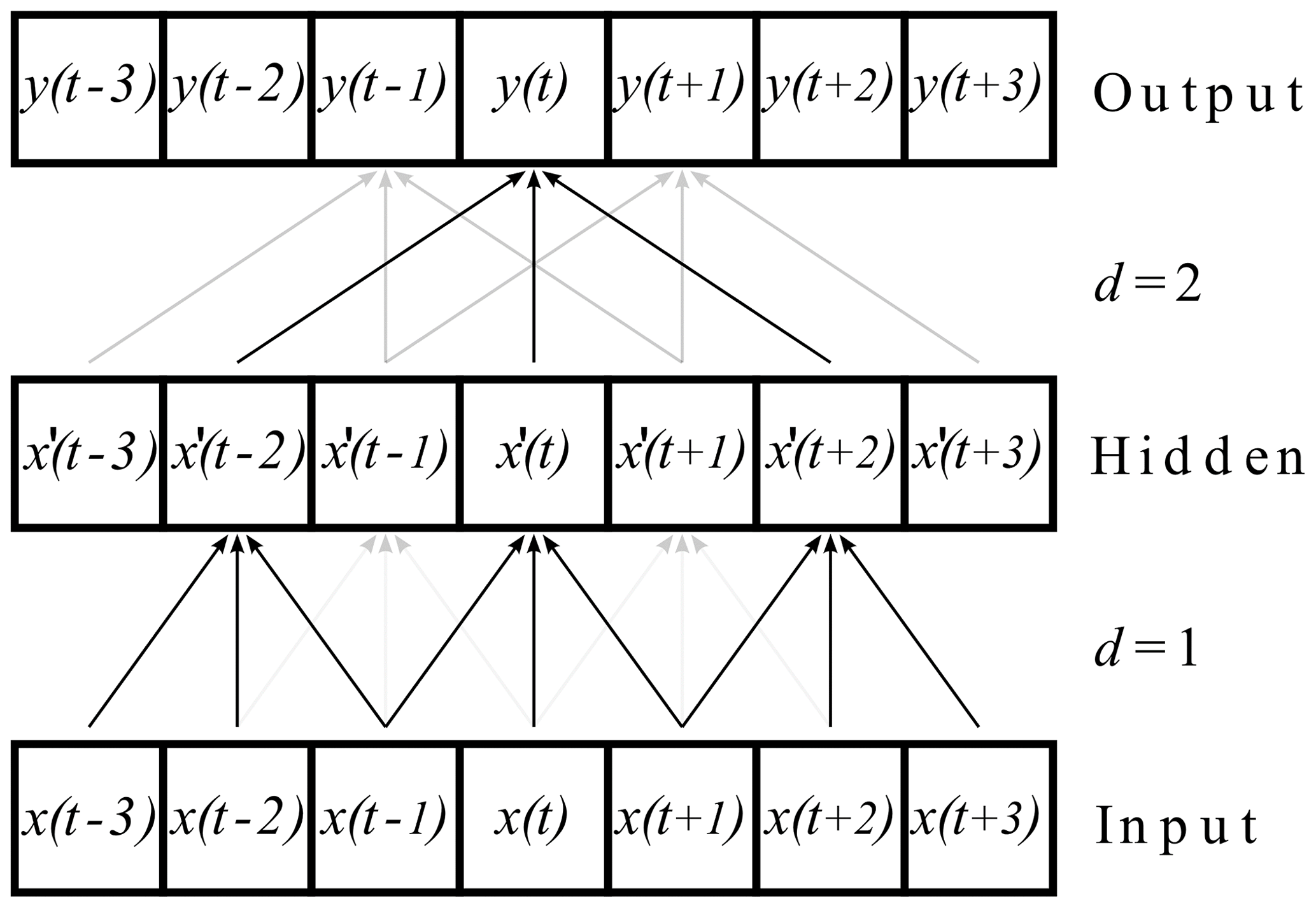
Figure 2 Stacked dilated convolutions applied to a time series x(t). The output is denoted with y(t). The dilated convolutions have the dilation factors $d=\mathrm{1},\mathrm{2}$ and a kernel of length 3 (according to Bai et al., 2018). In order to avoid a shortening of the time series in each step, the series are enlarged by zeros at the beginning and the end (also called zero padding).

We constructed and trained two TCN instances for different sequence lengths. The short sequence includes features of 13 time steps, which corresponds to a time of approximately 3 min. The long sequence includes features of 61 time steps, which corresponds to a time span of approximately 14 min. These two different sequence lengths were used so that one TCN (TCN₁₃), on one hand, has a way of reacting well to short-term events. On the other hand, the greater information content of a long sequence can be used, so the second TCN (TCN₆₁) can better classify unclear episodes. The two sequence lengths lead to two independent classifications by the respective TCN for the same point in time.

We always used a kernel size of 3 for the dilated convolutions. Furthermore, for the input sequence length of 13, the dilation factors for the TCN₁₃ were $d=\mathrm{1},\mathrm{2}$, while for the input sequence length of 61, the dilation factors for that TCN were $d=\mathrm{1},\mathrm{2},\mathrm{4},\mathrm{8}$. Comparing the given sequence length of 13 for the given dilation factors 1 and 2 with the sequence length from Fig. 2 for the same dilation factors, a difference between the theory and implementation can be noticed. This is a known property of the given implementation (https://github.com/philipperemy/keras-tcn/issues/207, last access: 21 June 2023, https://github.com/philipperemy/keras-tcn/issues/196, last access: 21 June 2023). The implementation always achieves a maximum sequence length with a dilation factor less than required in theory. For example, a maximum sequence length of 13 does not require the theoretical dilation factors of $d=\mathrm{1},\mathrm{2},\mathrm{4}$; it only requires $d=\mathrm{1},\mathrm{2}$.

The number of filters (number of different stacked dilated convolutions applied to every feature sequence) is 16. This results in approximately 3000 trainable parameters for TCN₁₃ and 6000 trainable parameters for TCN₆₁.

After describing the basic idea of a TCN as introduced in Bai et al. (2018), we also would like to give the most important information about the implementation of the TCN. For this the TCN used so-called residual blocks as described in Bai et al. (2018). A residual block consists of two hidden layers (each hidden layer comprises the weighting of the signals using dilated convolutions, the activation of the neurons and the processed signals) and a skip connection. The skip connection allows us to jump over hidden layers. As the activation function we used the rectified linear unit (ReLU) in the residual block (Nair and Hinton, 2010) and, due to the classification task, the softmax function in the output layer. Softmax ensures, among other aspects, that the individual values of the prediction vector, i.e., the output of the neural network, can be interpreted as a probability. The weights in the residual block are normalized during the training process with weight normalization as introduced in Salimans and Kingma (2016) and for temporal convolution networks suggested in Bai et al. (2018).

One challenge when using neural networks is to avoid overfitting; i.e., the network only memorizes the training data. In order to prevent this, we used a dropout regularization as proposed in Srivastava et al. (2014), with the ratio of 0.3 in the residual block as well as in the layer before the output layer. That means randomly 30 % of the inputs of neurons in each of these layers are switched off during the training of the network. Additionally, Gaussian noise is added to the time series before it is passed to the TCN. The architecture of our TCN is displayed in Fig. 3.

Figure 3 The input is a sequence of length 13 with 8 features at each time step. It has the dimensions 8 × 13. The first layer is a Gaussian noise layer, which is only active during training and adds slight normally distributed noise to the input data (standard deviation = 0.01). Afterwards the 8 × 13 data points are passed to the TCN and there to the first residual block. This residual block implements a 1-dimensional dilated convolution with a dilation factor of d= 1 and kernel length of 3. Since we have 16 filters (16 different initialized kernels), this also leads to 16 output features. The number of time steps remains the same. Afterwards, the same is repeated in the second residual block, only with the dilation factor increased to d= 2. The last step in the TCN is picking up the black-marked middle element of the 13 time steps since only this element contains information about the complete time sequence. This is done with the help of a so-called lambda layer. Finally, we map the 16 features resulting from the TCN to the three output neurons with a fully connected layer and the softmax function as the activation function. In this representation, the dropout regularization in the residual blocks as well as in the output layer (with a factor of 0.3) is not shown.

As mentioned at the beginning of this section, the class prediction of each image is stored in a vector. The length of the vector is equal to the number of classes. Since we have three classes, the vector is 3-dimensional. The ground truth classification vector has a single entry equal to 1 and two entries equal to zero because each image is manually assigned to a single label class. This kind of classification encoding is called a one-hot classification vector. The prediction vector of our learned classifier also has three entries, and every entry gives the predicted probability of the respective label class. We calculate the mean vector of the two prediction vectors for a sequence length of 13 and 61 and call this the “combined classifier”, whose entries can also be interpreted as a probability for the respective label class. To retrieve information about the quality of the classification and to learn, the difference between the classification vector and the prediction vector needs to be measured; this is done by the “categorical cross-entropy” metric which is explained in Murphy (2012). This is repeated for all inputs in a batch and the resulting average is called loss. This loss has to be minimized based on the adjustment of the trainable parameters (i.e., weights and biases of the different neurons), which can be done using a gradient-based optimizer. Our TCN was trained by the Adam optimizer, which was introduced in Kingma and Ba (2014). A starting learning rate of 0.05 provided the best results. The learning rate was additionally (to the adjustments of the Adam optimizer) adjusted at the beginning of all 100 training epochs in the following way: after each epoch the learning rate was reduced by a factor of exp(−0.2). After 25 epochs and multiples thereof, the learning rate was increased to approximately 70 % of the last maxima. This principle of such a so-called cycling learning rate was proposed in Smith (2017) and leads to the fact that only a range around the perfect learning rate has to be found instead of a perfectly fitting learning rate.

During the training process we saved the model with the lowest loss on the validation data, also estimated by the categorical cross-entropy metric.

Due to the large number of data, it is most important that sequences predicted as dynamic are actually dynamic episodes. This can be measured by the precision. The precision P_i of a label class i is the quotient of correctly positive predicted time steps of a label class $t_{{\mathrm{p}}_i}$ and all time steps that are assigned by the classifier to a label class (i.e., the sum of the correctly positive and the false positive predicted time steps $t_{{\mathrm{p}}_i}+f_{{\mathrm{p}}_i})$:

$$\begin{array}{}\text{(3)}& P_i={\displaystyle \frac{t_{{\mathrm{p}}_i}}{t_{{\mathrm{p}}_i}}}+f_{{\mathrm{p}}_i}.\end{array}$$

The counterpart to precision is recall R_i (of a label class i), which is calculated by dividing the correctly positive predicted time steps of a label class $t_{{\mathrm{p}}_i}$ by all the time steps manually assigned to a label class (i.e., the sum of the correctly positive predicted and the false negative predicted time steps $t_{{\mathrm{p}}_i}+f_{{\mathrm{N}}_i})$:

$$\begin{array}{}\text{(4)}& R_i={\displaystyle \frac{t_{{\mathrm{p}}_i}}{t_{{\mathrm{p}}_i}+f_{{\mathrm{N}}_i}}}.\end{array}$$

Therefore, recall is a measure of how many time steps of a label class are actually recognized by the classifier, whereas precision only evaluates the time steps assigned to a label class by the classifier and thereby determines the proportion of all correctly assigned time steps.

Thresholds can be defined to determine at what value a prediction is assigned to a label class. For example, if a threshold value of zero is set for the output neuron of the label class dynamic, all time steps will be assigned to the label class dynamic. In this case, the recall is at its maximum value of 1, whereas the precision is usually at its minimum, since there is normally a large number of false positive time steps. If the threshold value is now increased step by step, recall decreases and precision increases at the same time.

For each threshold value, a value pair of precision and recall can now be formed. Plotting recall versus precision and calculating the area under the curve, we get the so-called “average precision” (AP) of a respective label class, which can reach the maximum value of 1 (see Fig. 4). This is a reliable quality metric for the detection of a label class of a classifier independent of the thresholds used. Calculating the mean value of all average precision values, i.e., for calm, dynamic and cloudy, gives the mean average precision of a classifier.

3.5 Analysis of the classification algorithm

According to the precision–recall curves on the test data set (Fig. 4), the combined classifier achieves a mean average precision of 0.82. Taking a closer look at all average precision values reveals the following result.

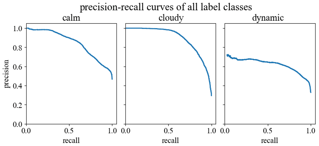
Figure 4 Precision–recall curves of all three label classes on the test data. Each value pair of precision and recall is based on a threshold value which decides whether a prediction is assigned to a label class or not. These thresholds start at a high level and are decreased constantly until a recall of 1.0 is achieved. This is done for all label classes separately. The area under the precision–recall curve is called the average precision (AP) of the label class.

The average precision for the actual target label class dynamic is 0.63. If we consider the same statistical measures on the non-target label classes calm and cloudy, we achieve an average precision of 0.85 for the label class calm and an average precision of 0.90 for the label class cloudy.

For our combined classifier, we used features instead of whole images. In order to determine the importance of individual features groups for detection, we derived the precision values by omitting one of the three groups of features (basic, texture and PSD features). If we omit the feature groups basic features or texture features, we only detect tiny changes in the average precision of the label classes calm and cloudy. The decrease in the average precision of the label class dynamic is a bit higher while omitting the basic feature group instead of the texture feature group. This leads to a slightly lower mean average precision by omitting the basic feature group compared to the texture feature group. The greatest influence on all statistical measures is the PSD feature group. Omitting this feature group leads to a decrease of approximately 10 % in every average precision value. Therefore, the mean average precision also decreases by approximately 10 %.

So far, we have reported the general metrics of the neural network. To sum it up, the prediction of the label class cloudy has given the best results, followed by calm and with some distance dynamic.

Since our goal is the identification of dynamic episodes, we adjusted the classification criteria to optimize the precision of the label class dynamic. This configuration was modified according to the validation data and tested on the test data in the final step. The classification criteria are specified as follows.

First, we set thresholds for whether predictions are assigned to a label class or not. This is done using Fig. 5, which shows the precision and recall for each label class as a function of the threshold values.

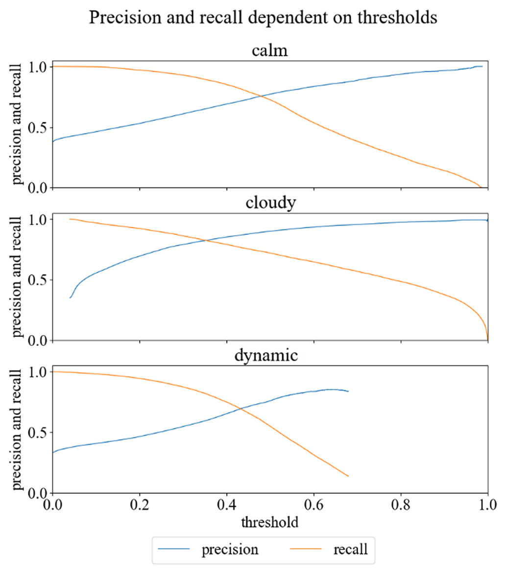
Figure 5 Precision and recall dependent on thresholds (on validation data) for all three label classes calm, cloudy and dynamic.

We have chosen threshold values 0.35 for the label class clouds and 0.5 for the label class calm, since the precision and recall of these two label classes are almost identical for these threshold values on the validation data set. For the label class dynamic we have chosen 0.5 as the threshold. In contrast to the other label classes, precision is higher than recall in order to optimize the precision of the label class dynamic. Due to these individual thresholds, it is possible that the final classifier suggests no label class or more than one label class for some time steps.

If time steps are not assigned to any label class, we classify them as “unsure”. If the classifier suggests more than one label class for a time step, the label class with the highest average precision wins the prediction.

Applying this procedure to the test data leads to the following confusion matrices and statistical measures (Tables 2, 3 and 4).

In confusion matrices, the manual classifications are plotted in the vertical direction and the automatic predictions in the horizontal direction. Correct predictions are therefore on the main diagonal, whereas incorrect predictions are on the secondary diagonal. This allows us to not only identify label classes that can be well distinguished, but also label classes that are more difficult to distinguish.

Table 2 Confusion matrix of the combined classifier, with thresholds of 0.35 for the label class cloudy, 0.5 for the label class calm and 0.5 for the label class dynamic. The bold values represent the diagonal of the confusion matrix, i.e., the number of points for which the predicted label is equal to the true label.

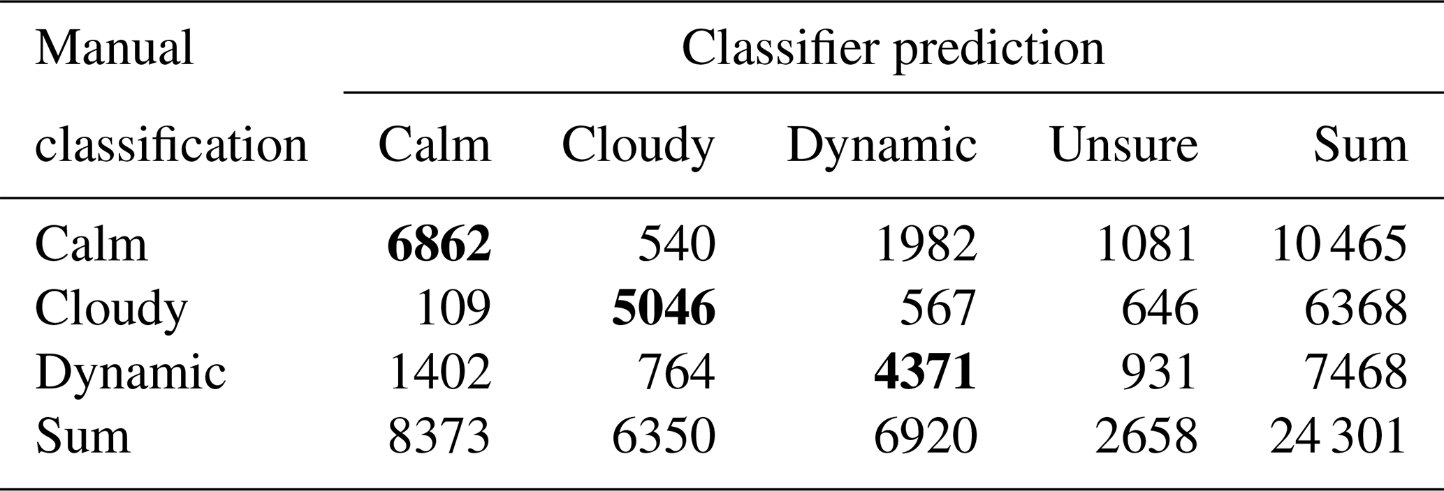
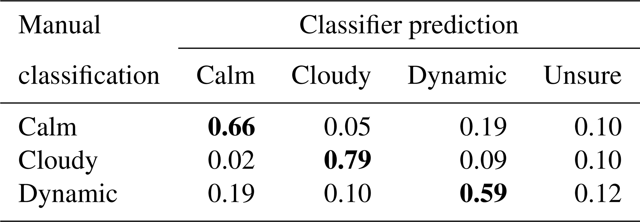
The confusion matrix displayed in Table 2 presents a detailed look at every manual classification and prediction of the combined classifier. As the number of manual classifications differs in each label class, drawing a conclusion on the quality of the classifier's predictions regarding the confusion of individual label classes is quite difficult. Therefore, we also display a normalized version of the confusion matrix in Table 3. Each row is normalized by the sum of each row, so the results in Table 3 are independent of the number of manual classifications in each label class.

Table 3 Normalized confusion matrix of the classifier displayed in Table 2. Each row in the confusion matrix is divided by the sum of the row, which is equal to the sum of classifications in the corresponding label class.

Before we go into the details of the confusion matrices in Tables 2 and 3, we briefly focus on the statistical measures which are calculated based on the confusion matrix in Table 2. The statistical measures precision, recall and overall accuracy are presented in Table 4.

Table 4 Statistical measures precision, recall and overall accuracy calculated by the confusion matrix of Table 2.

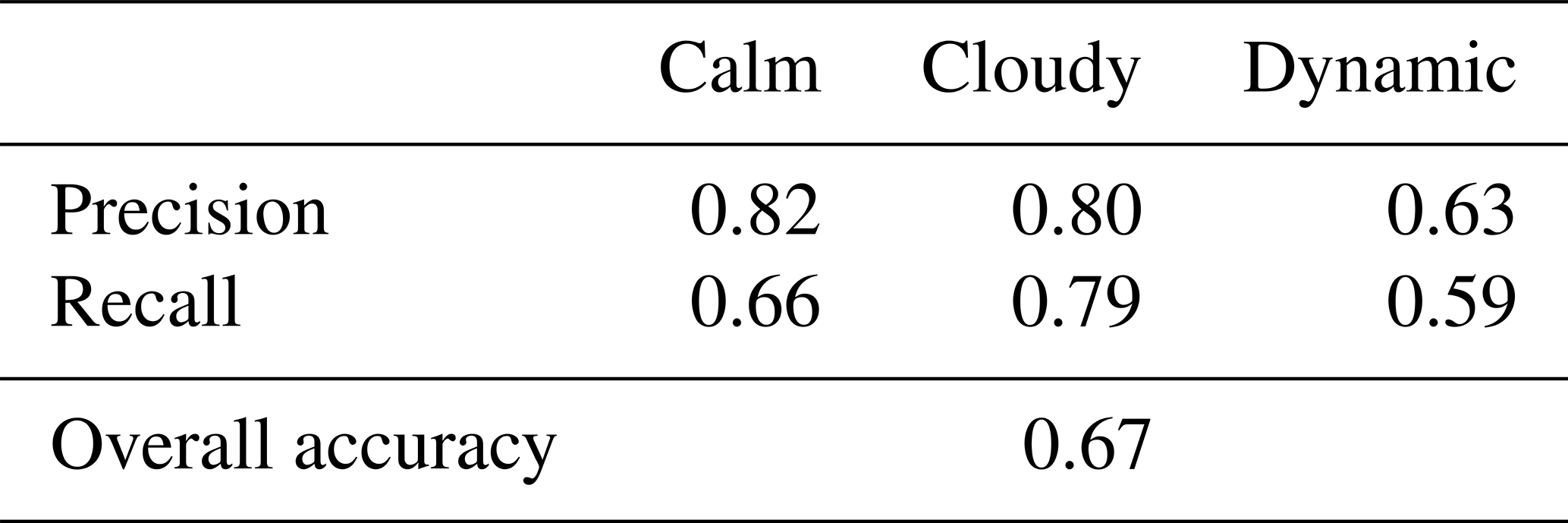
As we have seen before, Table 4 also shows that the combined classifier gives the best results for the label class cloudy, followed by calm and with some distance dynamic. There is just little difference between precision and recall in both label classes cloudy and dynamic, while the recall of the label class calm is much lower than its precision.

This is initially unexpected because we adjusted our thresholds in a way that recall and precision for the label classes calm and dynamic are almost on the same level. However, this can be explained by the confusion matrix in Tables 2 and 3. First, the label classes calm and dynamic have a high potential of being mixed up: 19 % of the episodes classified as calm are predicted as dynamic and vice versa. Secondly, all label classes occur at similar frequencies in the validation data set. So, if we compare this to the test data set, we can see (in the column “Sum”) that there are far more calm classifications than dynamic classifications. Combining these two aspects, it is on the one hand clear that the precision of the label class is boosted by the large number of calm classifications and therefore higher than the recall of the label class calm. On the other hand, a larger number of calm classifications leads (due to the high potential of mixed-up predictions between calm and dynamic) to a large number of predictions of dynamic which were originally classified as calm. This decreases the precision of the label class dynamic.

The confusion matrix in Table 2 suggests that there are in total more dynamic predictions which are originally classified with the label class calm than vice versa. But we have also seen that there are by far more calm classifications than dynamic classifications. Due to these aspects, the confusion matrix in Table 3 is normalized by the sum of each row, which means by the number of classifications of each label class. This confusion matrix shows that the proportion of mixed-up calm and dynamic timestamps in relation to the number of classifications of each label class is the same in both directions (19 % of the label classes calm or dynamic). It also shows that the lower recall of the label class dynamic (0.59) compared to the label class calm (0.66) is mainly caused by the increased number of cloudy predictions in relation to the total number of classifications when the timestamps are classified as dynamic.

It has been shown that the imbalance of the test data set and the mix-up between calm and dynamic predictions have a large influence on the statistical measures. Therefore, as a next step, calm predictions which are classified as dynamic and dynamic predictions which are classified as calm will be investigated. All these episodes are categorized as mispredicted or misclassified (Table 5).

Table 5 Overview of calm and dynamic episodes categorized as mispredicted and misclassified.

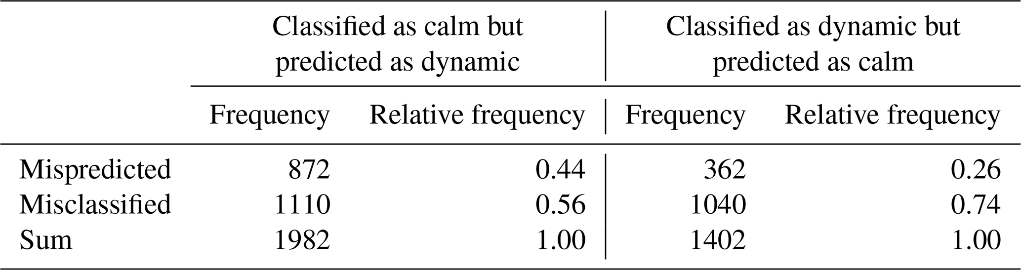
Table 5 shows that in both cases most of the time steps that are considered wrongly predicted are actually misclassified and not mispredicted. The relative frequency of mispredicted episodes is higher in the case of classified as calm but predicted as dynamic than in the opposite case. This can be partly explained by gravity wave structures, which are classified as dynamic and often predicted as calm, which leads to the assumption that our classifier or our features are not able to detect these structures.

In a further next step, the data classified as dynamic are used to find turbulence episodes. To determine the frequency of turbulence episodes in this label class, all sequences of the test data set predicted as dynamic were viewed and split into three categories: turbulence if rotating structures of nearly cylindrical shape can be detected, potentially turbulence if rotating structures can be suspected but not clearly detected and no turbulence if no structures can be observed that are relatable to rotating cylinders. Examples of these three categories can be seen in Video 1 (see video supplement to this article). The intervals of these three categories are discussed in detail within the next section.

Table 6 Categorization of all as dynamic predicted timestamps into three categories: turbulence, potentially turbulence and no turbulence.

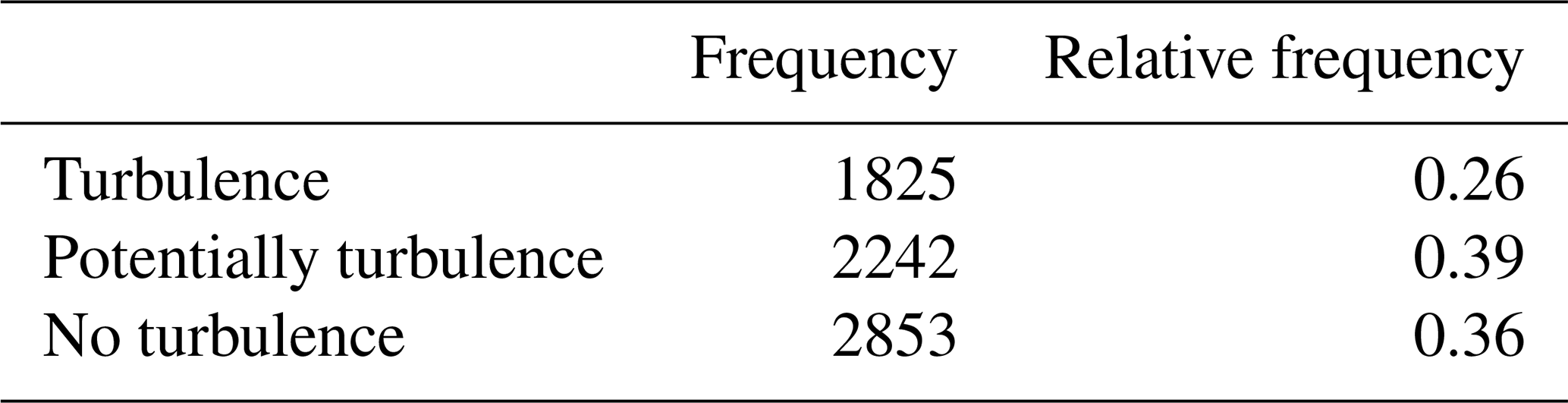
Splitting all as dynamic predicted timestamps in the described manner delivers three categories of roughly the same size (see Table 6). Slightly less than one-third contain turbulence. Another third contain structures that can be related to turbulence, and slightly more than one-third do not contain any structures that can be related to turbulence.

3.6 Discussion of the classification algorithm

At first glance, the statistical measures of mean average precision of 0.82 and average precision values of 0.90 for the label class cloudy, 0.85 for the label class calm and 0.63 for the label class dynamic on the test data set appear satisfying but not entirely convincing. In this context, a few aspects need to be considered. For instance, the fundamental task is not one of completely unambiguous class assignments (as it is in the case of basic object detections). In our case, the transitions between the label classes, in particular the transitions between calm and dynamic, are fluid. This also means that the manual classification is always subjective to some degree. Furthermore, there are events that are generally difficult to classify manually, such as very short cloud fields moving rapidly through the field of view or short calm (non-cloudy) episodes between cloud fields. To illustrate these aspects with an example, a video is digitally attached to the submission (Video 1). It shows the complete video footage of one night out of the test data set and is provided with the manual classification as well as with the raw and final automated prediction of the classifier (i.e., the manual classification is represented as a one-hot vector and the raw prediction is represented as a one-hot vector). In this video, some turbulent vortices are visible (19:30, 19:55, 20:10, 20:50; the time zone is UTC throughout the paper). These time periods are all correctly predicted as dynamic. Furthermore, the combined classifier detects even the smallest cloud veils, such as from 19:44–19:52. These are undoubtedly detectable but only faintly and briefly, so they were not noticed in the manual classification. In the statistics, this is counted as a false classification, as the labeling was incorrect.

The largest impact on the statistical measures is the confusion between calm and dynamic episodes (as shown in Tables 2 and 4). Video 1 in the video supplement also shows confused calm and dynamic episodes, especially episodes which are classified as dynamic but predicted as calm (22:06–22:14 and 22:23–22:45). Taking a closer look at these episodes reveals the difficulty of drawing boundaries between the label classes calm and dynamic. Nevertheless, episodes 22:06–22:14 and 22:33–22:45 can be considered misclassified, whereas the episode 22:23–22:33 is more likely to be considered mispredicted. Although only two of three episodes can be considered misclassified, all three episodes are counted as misclassification and formally impair the statistical measures of the classifier. So, in these cases it is mainly the manual classification that is wrong and not the prediction of the classifier. The prediction of the classifier also provides further advantages: the prediction of the classifier happens without significant time effort, whereas the manual classification of future data would take an extreme amount of time. In addition, it is not affected by human effects such as lack of concentration and subjectivity. This leads to the result in Table 5, which implies that the majority of confused calm and dynamic timestamps are caused by the manual classification due to misclassifications instead of mispredictions of the classifier. This leads to the fact that the classifier is better suited to distinguishing between calm and dynamic episodes than the manual classification. This confusion due to misclassification has the largest negative impact on precision and recall of the label class dynamic (listed in Table 4 and calculated according to Table 2) and is caused by errors in the manual classification (Table 5) and not by mispredictions of the classifier.

Assuming that the validation and training data sets contain the same proportion of calm and dynamic episodes that have been mixed up during the manual classification, it is worth saying that the training and validation data do not have to be perfectly classified (manually) in order to train a well-performing classifier.

The classification into three different label classes calm, dynamic and cloudy is a natural approach according to the video material. This does not automatically mean that this is a helpful search space restriction for the automated search for turbulence.

Looking at the relative frequencies of turbulence and potential turbulence (Table 6) reveals that about two-thirds of all data belonging to the label class dynamic can be of interest for turbulence analysis.

In the video shown in the video supplement, the intervals 19:28–19:30, 20:00–20:08, 20:22–20:25 and 21:16–21:29 are annotated with potential turbulence and the intervals 19:30–19:43, 19:52–20:01, 20:08–20:22 and 20:50–20:58 are episodes in which turbulence can be observed. In order to complete the annotations of the video, the sequences that have been annotated with no turbulence are the following: 20:25–20:35, 20:48–20:50, 20:58–21:02, 21:05–21:17, 21:30–22:05 and 22:12–22:23. It remains to be said that the classification into the three label classes calm, dynamic and cloudy can be regarded as quite reasonable, since in two-thirds of all dynamic timestamps, either turbulence or events resembling turbulence occur.

In future work, the resulting downsized data set (all data that are predicted as dynamic) can be used to train neural networks using image data to directly detect and potentially measure turbulence. This was not possible before due to several issues.

Firstly, the computational cost of processing image sequences in a neural network is higher than processing a time series of manually determined features of the images: a time series of images requires processing 10 000 data points per time step (if the image has a resolution of 100 × 100 pixels), whereas a time series of our features only requires processing 8 data points per time step. Using time series (with 13 and 61 steps respectively) instead of a single time step increases computational costs additionally. This will become crucial when applying this method to larger quantities of data.

Secondly, training with single images instead of image sequences to reduce computational cost is not ideal. Image sequences, in comparison to single images, contain essential information for the differentiation of the respective label classes. For example, cloud veils in a single image often cannot be distinguished from the label class dynamic, or turbulence vortices that appear similar to rotating cylinders can only be clearly identified by the information of the image sequence.

This reduced data set contains only episodes that show “dynamics” in the UMLT, of which approximately two-thirds are potentially related to turbulence. Thus, the data set is more balanced with respect to turbulence, which simplifies training for direct search and measurement of turbulence. Future work will also not waste computational time on calm and cloudy episodes (where observable turbulence is not expected), making training with the image sequences more efficient.

4 Analysis and discussion of turbulence

Checking the dynamic episodes from the TCN model by hand, we identified 19 episodes of turbulence. Of them, 13 exhibited such a good quality that we were able to read out the length scale and the root-mean-square velocity of turbulence and calculate the energy dissipation rate ϵ, according to the method applied by Hecht et al. (2021) and Sedlak et al. (2021). The resulting values are displayed in Table 7. The uncertainty δϵ is calculated by applying the rules of error propagation to Eq. (1). Similarly to Sedlak et al. (2021), a general read-out error of ±3 pixels is used. This leads to an uncertainty in the length scale δL of ±69 m and (since velocities are determined over a set of 10 images) an uncertainty in the velocity δU of ±2.5 m s⁻¹.

Table 7 Values of the energy dissipation rate ϵ and the corresponding uncertainty δϵ of all turbulence events of sufficient quality found in the airglow image data between 11 June 2019 and 25 February 2020 acquired at Oberpfaffenhofen, Germany.

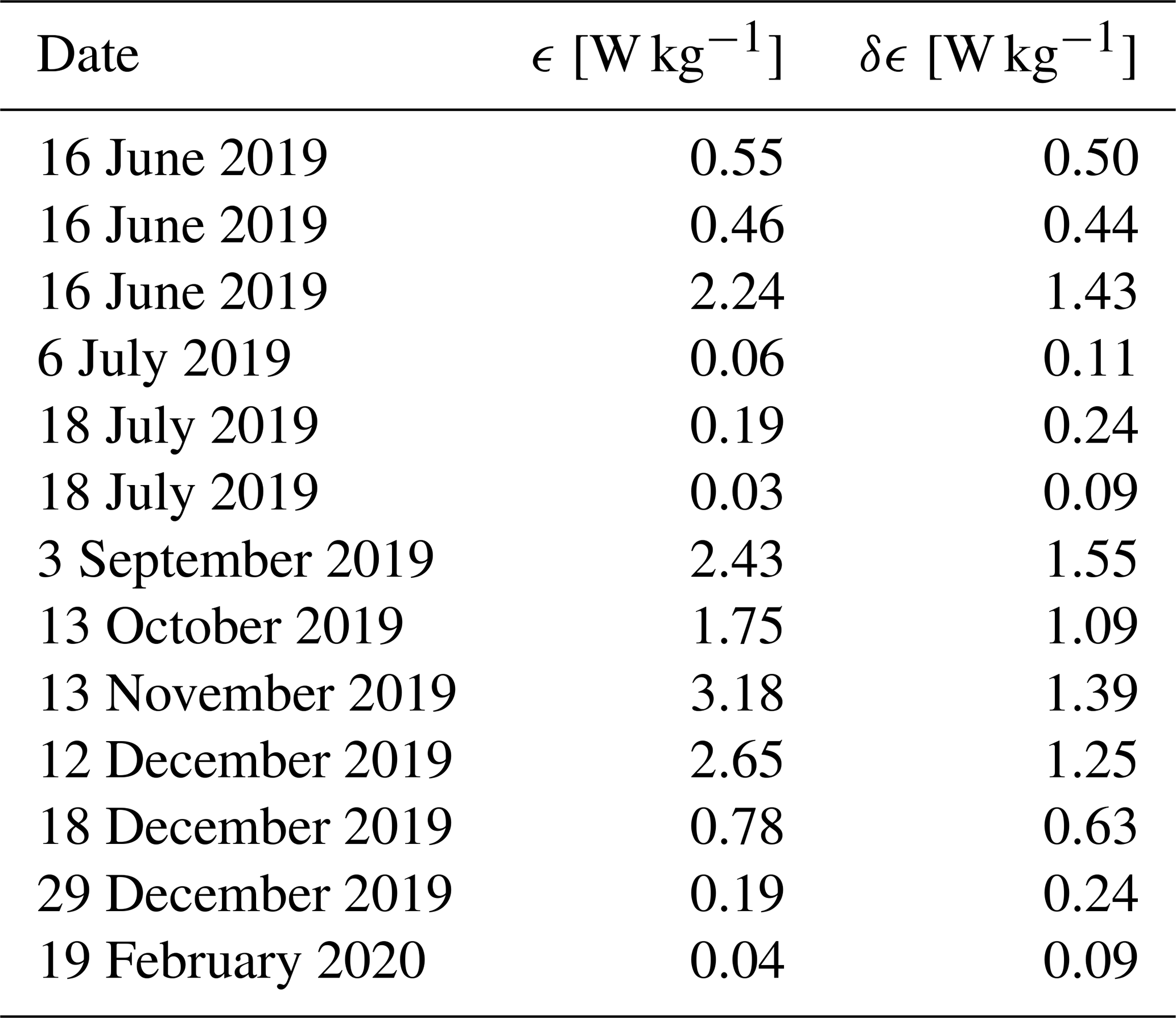
The values of ϵ range from 0.03 to 3.18 W kg⁻¹ with a median value of 0.55 W kg⁻¹ and a standard deviation of 1.16 W kg⁻¹. In Sedlak et al. (2021), for comparison, ϵ ranges from 0.08 to 9.03 W kg⁻¹ with a median value of 1.45 W kg⁻¹. In both studies, the values cover 3 orders of magnitude; however this is also reflected in the publications of other authors. Hecht et al. (2021) found an energy dissipation rate of 0.97 W kg⁻¹ with this approach; Chau et al. (2020) present an energy dissipation rate of 1.125 W kg⁻¹ and claim that this would be a rather high value. Hocking (1999) finds a maximum order of magnitude of 0.1 W kg⁻¹.

Although the identification of turbulent episodes is done automatically via the TCN approach presented in Sect. 3, the measurement of L and U is still done manually. This implies an inherent read-out uncertainty due to the blurry structures and a remaining possibility of misinterpretation, which we intended to minimize by multiple-eye inspection of the episodes. It is interesting to note that no events with very large energy dissipation rates in the range 4–9 W kg⁻¹ as in Sedlak et al. (2021) were found in this data set, whereas the lower limit of ϵ is quite similar. It is still an open question whether the larger values are the result of direct energy dissipation or if the respective large eddies are about to further decompose into smaller structures beyond the sensitivity of our instrument, which then mark the actual end of the energy cascade.

The values in Table 6 are in good agreement with literature values; however the database is still very small. Future measurements of airglow imagers will have to be analyzed with the method applied here in order to establish reliable statistical conclusions.

5 Summary and outlook

We have investigated the application of practical and easy-to-use algorithms based on neural networks (NNs) to facilitate the detection of episodes showing turbulent motions in OH^* airglow image data. This is done by setting up two variants of a TCN (temporal convolutional neural network) to automatically pre-sort the images into images exhibiting strong airglow dynamics (where turbulence can likely be found), images exhibiting calm airglow or images disturbed by clouds (which can be excluded from further turbulence analyses). The image data used in this work were acquired by the high-resolution camera system FAIM 3 at Oberpfaffenhofen, Germany, between 11 June 2019 and 25 February 2020.

The TCN-based classification algorithm (based on the time series of features derived from the temporal image sequences) achieves a mean average precision of 0.82. We demonstrated with a video example from the test data set that the algorithm works much better than the statistical values suggest. A total of 13 episodes exhibit a sufficiently high quality to derive the energy dissipation rate ϵ. Values range from 0.03 to 3.18 W kg⁻¹ and are in good agreement with previous work. The data analyzed here confirm the importance of considering dynamically driven energy deposition by breaking gravity waves when studying the energy budget of the atmosphere.

We have shown that an NN-based algorithm can support the identification of turbulent episodes in airglow imager data. This marks an important step in expanding the method of extracting turbulence parameters from airglow images. Utilizing neural networks is a promising way of dealing with “big data”. With ongoing airglow measurements, it will be possible to also investigate effects like seasonal or latitudinal variations in the energy dissipation rate with diminishing uncertainties.