Estimation of secondary organic aerosol formation parameters for the volatility basis set combining thermodenuder, isothermal dilution, and yield measurements

Secondary organic aerosol (SOA) is a major fraction of the total organic aerosol (OA) in the atmosphere. SOA is formed by the partitioning onto pre-existent particles of low-vapor-pressure products of the oxidation of volatile, intermediate-volatility, and semivolatile organic compounds. Oxidation of the precursor molecules results in a myriad of organic products, making the detailed analysis of smog chamber experiments difficult and the incorporation of the corresponding results into chemical transport models (CTMs) challenging. The volatility basis set (VBS) is a framework that has been designed to help bridge the gap between laboratory measurements and CTMs. The parametrization of SOA formation for the VBS has been traditionally based on fitting yield measurements of smog chamber experiments. To reduce the uncertainty in this approach, we developed an algorithm to estimate the SOA product volatility distribution, effective vaporization enthalpy, and effective accommodation coefficient combining SOA yield measurements with thermograms (from thermodenuders) and areograms (from isothermal dilution chambers) from different experiments and laboratories. The algorithm is evaluated with “pseudo-data” produced from the simulation of the corresponding processes, assuming SOA with known properties and introducing experimental error. One of the novel features of our approach is that the proposed algorithm estimates the uncertainty in the predicted yields for different atmospheric conditions (temperature, SOA concentration levels, etc.). The uncertainty in these predicted yields is significantly smaller than that of the estimated volatility distributions for all conditions tested.

1 Introduction

Submicrometer atmospheric particles are of great importance due to their negative effects on public health (Pope and Dockery, 2006; Lim et al., 2012) and their uncertain influence on Earth's climate (IPCC, 2021). Organic aerosol (OA) contributes 20 %–90 % of the submicron particulate mass (Zhang et al., 2007) and is emitted directly into the atmosphere as primary organic aerosol (POA) or formed as secondary organic aerosol (SOA). SOA constitutes a major fraction of the total OA in the atmosphere, contributing more than 60 % on average (Kanakidou et al., 2005). SOA is formed by the condensation of low-vapor-pressure products of the oxidation of volatile organic compounds (VOCs), intermediate-volatility organic compounds (IVOCs), and semivolatile organic compounds (SVOCs).

Hundreds of mostly unknown products are formed during the oxidation of each SOA precursor, making the detailed description of the corresponding reactions and eventual SOA formation extremely challenging. The volatility basis set (VBS) is one approach that has been proposed to simplify the system and to allow SOA simulation in chemical transport models (CTMs). The VBS describes the volatility distribution of OA using a set of surrogate species with effective saturation concentrations that vary by 1 order of magnitude (Donahue et al., 2006; Stanier et al., 2008). Volatility is one of the most important physical properties of SOA components as it determines to a large extent their gas–particle partitioning (Pankow, 1994a, b). The parametrization of SOA formation for the VBS requires the determination of the yields of each volatility bin (volatility distribution of products) and the corresponding enthalpies of vaporization.

The SOA parametrizations for the VBS have been traditionally based on fitting yield measurements (Lane et al., 2008). The major weakness of this approach is that the resulting parametrization is limited to the range of OA concentrations and temperatures of the measurements. In most cases, the concentration range does not include the low concentrations relevant to the atmosphere, and usually most of the experiments take place in a relatively narrow temperature range. Pathak et al. (2007a) needed 37 smog chamber experiments at different temperatures (0–45 ^∘C) and atmospherically relevant concentrations to constrain the α-pinene SOA temperature sensitivity.

A number of approaches have been used to minimize the number of experiments needed to characterize the temperature dependence of the SOA formation. Stanier et al. (2007) developed an experimental technique with which the temperature-controlled smog chamber could be heated or cooled after the SOA formation, moving the system to new equilibrium favoring evaporation or condensation respectively. However, interactions of the SOA with the walls of the system increased the uncertainties in the approach. Stanier et al. (2008) presented an algorithm to fit the smog chamber experiments using several volatility bins. However, the number of experiments needed by the algorithm should cover a wide range of concentrations and temperatures to effectively constrain the stoichiometric mass yields and the effective vaporization enthalpy.

In an effort to cover a wider concentration and temperature range, thermodenuder measurements can be used. The thermodenuder (TD) is a common instrument developed to characterize the volatility of atmospheric aerosols by heating them and observing the resulting changes in size, mass, optical properties, etc. (Burtscher et al., 2001; Wehner et al., 2002, 2004; An et al., 2007). TDs consist of a heated tube in which the volatile particle components evaporate followed by a cooling section with activated carbon to avoid vapor recondensation. The mass changes in TDs depend on the initial SOA concentration, the residence time in the heating tube, the vaporization enthalpy, and the mass transfer resistances. The latter are described by the effective accommodation coefficient that has been traditionally used to account for resistances to mass transfer not only at the surface of the particle but also inside the particle. The evaporation rate for most particles is relatively insensitive to its value when this value is around 1. A typical way of reporting the TD measurements is by calculating the aerosol mass fraction remaining (MFR) at a given temperature after passing through the TD. The MFRs in a range of TD temperatures constitute the thermogram.

In applications in the field (Cappa and Jimenez, 2010; Huffman et al., 2009; Lee et al., 2010; Louvaris et al., 2017a) and in the laboratory (Kalberer et al., 2004; Baltensperger et al., 2005; An et al., 2007; Lee et al., 2011; Cain et al., 2020), the particles do not reach equilibrium with the gas phase inside the TD. Therefore, dynamic aerosol evaporation models (Riipinen et al., 2010; Cappa, 2010; Fuentes and McFiggans, 2012) are needed for the interpretation of TD measurements. Karnezi et al. (2014) used the time-dependent evaporation model of Riipinen et al. (2010) to calculate the OA volatility distribution, vaporization enthalpy, and mass accommodation coefficient from TD measurements. The authors showed that a simple error minimization approach may not be appropriate for such systems as very similar thermograms can be obtained for multiple combinations of different parameters. For this reason, their approach estimates an ensemble of “good” solutions, from which the best estimate and the corresponding uncertainties are derived.

Grieshop et al. (2009) suggested the combination of TD and isothermal dilution to constrain the volatility distribution of SOA. Karnezi et al. (2014) proposed an algorithm to include both types of measurement. The authors concluded that the combination of the two types of measurement can better constrain the OA volatility than each set separately. Louvaris et al. (2017b) and Cain et al. (2020) applied this algorithm to cooking OA (COA) and SOA respectively. Louvaris et al. (2017b) showed that the use of only TD measurements led to overestimation of the SVOC fraction of COA, while the use of TD and isothermal dilution data reduced the uncertainty in the volatility distribution and the effective vaporization enthalpy. Cain et al. (2020) conducted TD and isothermal dilution experiments for α-pinene and cyclohexene ozonolysis SOA. The SOA in these two systems had similar thermograms but different areograms. When only thermograms were used in the model, the volatility distributions were quite similar. However, the addition of areograms revealed that α-pinene ozonolysis SOA consists mostly of low-volatility organic compounds (LVOCs) and the cyclohexene ozonolysis SOA consists mostly of SVOCs.

To constrain the volatility product distribution of SOA and its effective vaporization enthalpy, we combine TD and isothermal dilution experiments with the SOA yield measurements. We extend here the algorithm of Karnezi et al. (2014) by introducing additional inputs (SOA yields) and by providing additional outputs (uncertainty in estimated yields in relevant atmospheric conditions). The algorithm is tested with “pseudo-experimental” data generated from the use of models simulating the corresponding measurement processes; therefore the true parameters are known. The results of the “pseudo-experiments” are corrupted so that they include experimental errors.

2 Model description

2.1 SOA formation

Gas-phase oxidation of VOCs involves a large number of reactions and produces a large number of products that can condense in the particulate phase. Depending on their effective saturation concentration, they can be represented in the 1D VBS framework by

$$\begin{array}{}\text{(1)}& \begin{array}{rl}\mathrm{VOC}+\mathrm{oxidant}\to & {\mathit{\alpha }}_{\mathrm{1}}{P}_{\mathrm{1}}+{\mathit{\alpha }}_{\mathrm{2}}{P}_{\mathrm{2}}+\mathrm{\dots }+{\mathit{\alpha }}_n{P}_n\\ & +\mathrm{volatile}\mathrm{products},\end{array}\end{array}$$

where n is the number of the surrogate compounds (volatility bins in the VBS), P_i is the surrogate product in the ith volatility bin, and α_i is the corresponding stoichiometric mass yield. The total SOA mass yield can be then calculated as

$$\begin{array}{}\text{(2)}& Y\equiv {\displaystyle \frac{C_{\mathrm{OA}}}{\mathrm{\Delta }\mathrm{VOC}}}=\sum _i^n{\displaystyle \frac{{\mathit{\alpha }}_i}{\mathrm{1}+\left(C_i^{\ast }/C_{\mathrm{OA}}\right)}},\end{array}$$

where C_OA is the total SOA concentration, ΔVOC is the consumed concentration of the VOC, and $C_i^{\ast }$ is the effective saturation concentration of compound i. This yield equation is an extension of the two-product model by Odum et al. (1996), replacing their semi-empirical partitioning coefficients with the assumption of a pseudo-ideal solution (Strader et al., 1999). This model assumes that the system has reached equilibrium when the yield is measured and that the differences in molecular weights are small.

The effective saturation concentrations at different temperatures are given by the Clausius–Clapeyron equation:

$$\begin{array}{}\text{(3)}& C_i^{\ast }\left(T\right)=C_i^{\ast }\left(T_{\mathrm{ref}}\right){\displaystyle \frac{T_{\mathrm{ref}}}{T}}\exp \left[{\displaystyle \frac{\mathrm{\Delta }{H}_{\mathrm{vap},i}}{R}}\left({\displaystyle \frac{\mathrm{1}}{T_{\mathrm{ref}}}}-{\displaystyle \frac{\mathrm{1}}{T}}\right)\right],\end{array}$$

where T_ref is the reference temperature in which the reference effective saturation concentration is defined (298 K in this work) and ΔH_vap,i is the enthalpy of vaporization of surrogate compound i.

2.2 Thermodenuder model

The time-dependent evaporation of SOA in the TD used in this work is described by the dynamic mass transfer model of Riipinen et al. (2010). The evolution of the total particle mass, m_p, and the gas-phase concentration of the compound i, C_i, are given by

$$\begin{array}{}\text{(4)}& {\displaystyle \frac{\mathrm{d}{m}_{\mathrm{p}}}{\mathrm{d}t}}=-\sum _{i=\mathrm{1}}^n{I}_i,\text{(5)}& {\displaystyle \frac{\mathrm{d}{C}_i}{\mathrm{d}t}}=I_i{N}_{\mathrm{tot}},\end{array}$$

where n is the number of surrogate compounds, N_tot is the total number concentration of particles (assuming a monodisperse aerosol population), and I_i is the mass flux of compound i from the gas to the particulate phase for each particle calculated by (Seinfeld and Pandis, 2016)

$$\begin{array}{}\text{(6)}& I_i={\displaystyle \frac{\mathrm{2}\mathit{\pi }{d}_{\mathrm{p}}{M}_i{\mathit{\beta }}_{\mathrm{m}i}{D}_i}{R{T}_{\mathrm{TD}}}}\left(p_i-p_i^{\mathrm{0}}\right).\end{array}$$

Here d_p is the particle diameter, R is the ideal gas constant, M_i is the molecular weight of compound i, D_i is the diffusion coefficient of compound i in the gas phase at temperature T_TD, p_i and $p_i^{\mathrm{0}}$ are the partial vapor pressures of i far away from the particle and at the particle surface respectively, and β_mi is a factor for the correction of kinetic and transition regime effects (Fuchs and Sutugin, 1970):

$$\begin{array}{}\text{(7)}& {\mathit{\beta }}_{\mathrm{m}i}={\displaystyle \frac{\mathrm{1}+{\mathit{Kn}}_i}{\mathrm{1}+\left(\frac{\mathrm{4}}{\mathrm{3}{\mathit{\alpha }}_{\mathrm{m}i}}+\mathrm{0.377}\right){\mathit{Kn}}_i+\frac{\mathrm{4}}{\mathrm{3}{\mathit{\alpha }}_{\mathrm{m}i}}{\mathit{Kn}}_i}}.\end{array}$$

Here Kn_i is the Knudsen number of compound i and α_mi is the mass accommodation coefficient of compound i on the particles. The partial vapor pressure of compound i at the particle surface is given by

$$\begin{array}{}\text{(8)}& p_i^{\mathrm{0}}=x_{\mathrm{m}i}{\displaystyle \frac{C_i^{\ast }RT}{M_i}}\exp \left({\displaystyle \frac{\mathrm{4}{M}_i\mathit{\sigma }}{R{T}_{\mathrm{TD}}\mathit{\rho }{d}_{\mathrm{p}}}}\right),\end{array}$$

where x_mi is the mass fraction of compound i in the particulate phase, $C_i^{\ast }$ is the effective saturation concentration, σ is the surface tension (assumed to be 0.05 N m⁻¹ in our simulations), T_TD is the particle temperature assumed to be the same as in the TD, and ρ is the particle density. The effective saturation concentrations at different TD temperatures are given by Eq. (3).

Processes other than organic aerosol evaporation may affect the TD measurements. For example, thermal decomposition may accelerate the transfer of organic compounds from the particulate to the gas phase and may lead to overestimation of the volatility of especially the least volatile components of the SOA (Epstein et al., 2010; Saha and Grieshop, 2016; Stark et al., 2017). However, the corresponding parameters for the SVOCs and the more volatile LVOCs that are important for atmospheric SOA modeling should be a lot less uncertain given that they are measured in relatively low TD temperatures. The use of isothermal dilution measurements may also help identify cases in which the model does not include a process (e.g., thermal decomposition) that dominates the behavior of the aerosol during heating. In this case, one expects that the overall algorithm will have difficulties reproducing all measurements (yields, isothermal dilution, and evaporation in the TD).

2.3 Isothermal dilution model

In isothermal dilution experiments, an SOA sample is injected into a reactor filled with clean air at room temperature. The concentrations of both the gas- and the particulate-phase components are lowered due to dilution leading the system out of equilibrium. The evaporation of SOA as a result of isothermal dilution is also described by Eqs. (3)–(8) (Karnezi et al., 2014), but the temperature is equal to 298 K. Evaporation in a dilution chamber depends on the initial SOA mass, time, and α_m but not on ΔH_vap as the particles evaporate without a change in temperature.

The dilution ratio is an important parameter, varying typically from 10 to 20 in SOA experiments (Cain et al., 2020). Low dilution ratios result in little evaporation and little signal to be explored by the parameter estimation algorithm. High dilution ratios lead to very low initial concentrations in the dilution chamber and a lot of noise in the subsequent evaporation measurements.

3 Algorithm for the estimation of VBS parameters

The algorithm of Karnezi et al. (2014) was first extended to include an SOA partitioning model described by Eqs. (1)–(3) together with the TD and isothermal dilution models in order to estimate the volatility product distribution, vaporization enthalpy, and accommodation coefficient. We discretized the domain of the parameters and simulated all combinations of stoichiometric mass yields (α_i), ΔH_vap, and α_m. The yields α_i were allowed to vary from 0.0 to 0.8, with values of 0.0, 0.05, 0.1, 0.15, 0.2, 0.3, 0.4, 0.6, and 0.8. The user of the algorithm can specify an upper limit for the sum of the yields to reduce the number of the potential solutions that the algorithm will test. Combinations with the sum of the yields exceeding 1.0 were excluded from the analysis originally. The sensitivity of our results to setting the upper limit of the sum of the yields equal to 2 is examined in Sect. 4.6. For a four-product system there are 3153 and for a six-product system 66 636 acceptable combinations. The values used for ΔH_vap were from 20 to 200 kJ mol⁻¹ with a step of 20, and for α_m, the values used were 0.001, 0.01, 0.1, and 1. As a result 126 120 simulations are needed (computational time of about 15 h on an office PC) for a four-product VBS and 2 665 440 for a six-product solution.

For each simulation and each type of measurement, we calculated the normalized mean square error (NMSE) defined as

$$\begin{array}{}\text{(9)}& \mathrm{NMSE}={\displaystyle \frac{\sum _{i=\mathrm{1}}^{N_{\mathrm{O}}}{\left(P_i-O_i\right)}^{\mathrm{2}}}{\sum _{i=\mathrm{1}}^{N_{\mathrm{O}}}{O}_i}},\end{array}$$

where O_i represents the ith observed value (corresponding to a specific SOA concentration for yield measurements, temperature for TD, or time for isothermal dilution), P_i the corresponding model-predicted value, and N_O is the total number of observations from each type of measurement. For each simulation (denoted as s), the overall error was calculated by assuming equal weight to the set of yield, TD, and dilution measurements and summing the corresponding errors:

$$\begin{array}{}\text{(10)}& E_s={\mathrm{NMSE}}_{Y,s}+{\mathrm{NMSE}}_{\mathrm{TD},s}+{\mathrm{NMSE}}_{\mathrm{Dil},s}.\end{array}$$

The parameter combinations for which the overall error E_s is less than 5 % are identified. The best solution is then calculated by averaging these solutions using the inverse error E_s as a weighting factor. The solutions that are closer to the measurements have higher weight. Therefore, for every combination of α_i, ΔH_vap, and α_m, the algorithm calculates one overall NMSE following Eq. (10) and all data points for each solution get the same weighting factor. More specifically the best estimate $\stackrel{\mathrm{‾}}{x}$ is given by

$$\begin{array}{}\text{(11)}& \stackrel{\mathrm{‾}}{x}={\displaystyle \frac{\sum _k^N{x}_k\frac{\mathrm{1}}{E_k}}{\sum _k^N\frac{\mathrm{1}}{E_k}}},\end{array}$$

where x_k is the estimated value of a property (mass yield of a volatility bin, effective vaporization enthalpy, or effective accommodation coefficient) and N is the number of combinations with error below the threshold value. The uncertainty range of the parameters is estimated by calculating the standard deviation (σ) following Karnezi et al. (2014):

$$\begin{array}{}\text{(12)}& \mathit{\sigma }=\sqrt{{\displaystyle \frac{\sum _k^N\left[{\left(x_k-\stackrel{\mathrm{‾}}{x}\right)}^{\mathrm{2}}\cdot \frac{\mathrm{1}}{E_k}\right]}{\sum _k^N\frac{\mathrm{1}}{E_k}}}}.\end{array}$$

4 Testing of the algorithm

4.1 Generation of data for evaluation

In order to evaluate the algorithm, we generated data using the output of SOA formation, thermodenuder and isothermal dilution models described in Sect. 2 for systems with known volatility distribution of the products and properties. Then, these data were “corrupted” with random errors to represent the “noise” observed in laboratory measurements for yields, thermograms, and areograms. As a result, there is no set of model parameters that can reproduce all the measurements. The yields were corrupted based on the variability in laboratory measurements of Pathak et al. (2007a), by assuming a normal distribution and standard deviation (σ_Y) given by

$$\begin{array}{}\text{(13)}& {\mathit{\sigma }}_Y=\mathrm{0.1}{Y}_{\mathrm{true}}+\mathrm{0.02},\end{array}$$

where Y_true denotes the correct yields.

For TD, the errors were calculated by assuming a normal distribution and the standard deviation (σ_TD) suggested by Karnezi et al. (2014):

$$\begin{array}{}\text{(14)}& {\mathit{\sigma }}_{\mathrm{TD}}=\mathrm{0.51}{\mathrm{MFR}}_{\mathrm{TD},\mathrm{true}}-\mathrm{0.5}{\left({\mathrm{MFR}}_{\mathrm{TD},\mathrm{true}}\right)}^{\mathrm{2}},\end{array}$$

where MFR_TD,true denotes the correct MFR values for each TD temperature.

For dilution, the errors were calculated by assuming a uniform distribution and standard deviation (σ_Dil) suggested by Karnezi et al. (2014):

$$\begin{array}{}\text{(15)}& {\mathit{\sigma }}_{\mathrm{Dil}}=\mathrm{0.05}{\mathrm{MFR}}_{\mathrm{Dil},\mathrm{true}}+\mathrm{0.03},\end{array}$$

where MFR_Dil,true denotes the correct MFR values for isothermal dilution.

Based on the above methodology, we generated “pseudo-measurements” of yield, TD, and isothermal dilution for different SOA systems. The parameters used to produce the pseudo-experimental data are summarized in Table S1 in the Supplement. The “experimental” conditions assumed for the TD and isothermal dilution measurements are shown in Table S2.

Figure 1 Measurements of Test A1 in Experiment A (red dots) and true (red line) and estimated (blue line) yields at (a) 5 ^∘C, (b) 15 ^∘C, (c) 25 ^∘C, and (d) 35 ^∘C, with (e) TD (thermogram) and (f) dilution (areogram) values. The grey area shows the range of good solutions obtained by our algorithm.

In Experiment A, we test the performance of the algorithm against α-pinene ozonolysis data and examine the effect of TD and isothermal dilution data. For Experiment A, the “true” values were taken from the parametrization derived by Pathak et al. (2007b) for the ozonolysis of α-pinene under low-NO_x and dark and low-RH conditions. Therefore, these results are good fits of the measurements analyzed in that study. The parametrization was derived assuming a four-volatility-bin system with saturation concentrations ranging from 1 to 10³ µg m⁻³. The effective vaporization enthalpy estimated in that study was equal to 30 kJ mol⁻¹. Because the effective accommodation coefficient was not part of the Pathak et al. (2007b) parametrization, we assumed a value of 0.5 in this work. We used a small number of yield measurements at atmospherically relevant SOA concentrations of 1, 5, 10, 20, and 40 µg m⁻³ (Fig. 1). For this SOA system, the yield at 40 µg m⁻³ did not exceed 20 %. The thermogram includes 10 MFR data points in the temperature range of 20 to 200 ^∘C. For the highest temperature, more than 70 % of the SOA mass was evaporated. The areogram shows that the corresponding SOA evaporated by almost 70 % in the first 0.5 h and more than 90 % in less than 3 h.

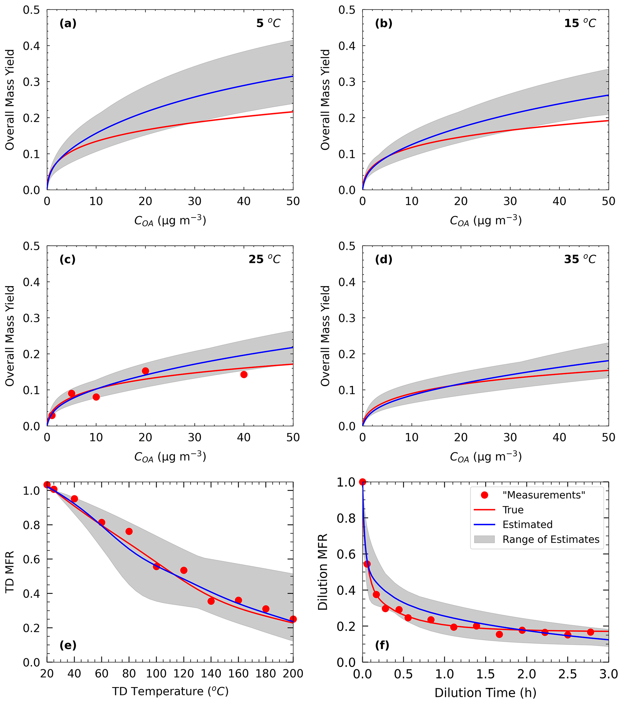
Figure 2 Measurements of Test B1 in Experiment B (red dots) and true (red line) and estimated (blue line) yields at (a) 5 ^∘C, (b) 15 ^∘C, (c) 25 ^∘C, and (d) 35 ^∘C, with (e) TD (thermogram) and (f) dilution (areogram) values. The grey area shows the range of good solutions.

For Experiment B, the true values were taken from the alternative parametrization proposed by Pathak et al. (2007b) for the same oxidation system as described before. This time, the authors used a seven-volatility-bin system with saturation concentrations ranging from 10⁻² to 10⁴ µg m⁻³ in their parametrization. The effective vaporization enthalpy of the parametrization was 30 kJ mol⁻¹, while for the accommodation coefficient we assumed again a value of 0.5. The yield, TD, and isothermal dilution measurements of Experiment B are generated in the same SOA mass concentration, temperature, and dilution time range as in the previous pseudo-experiment (Fig. 2).

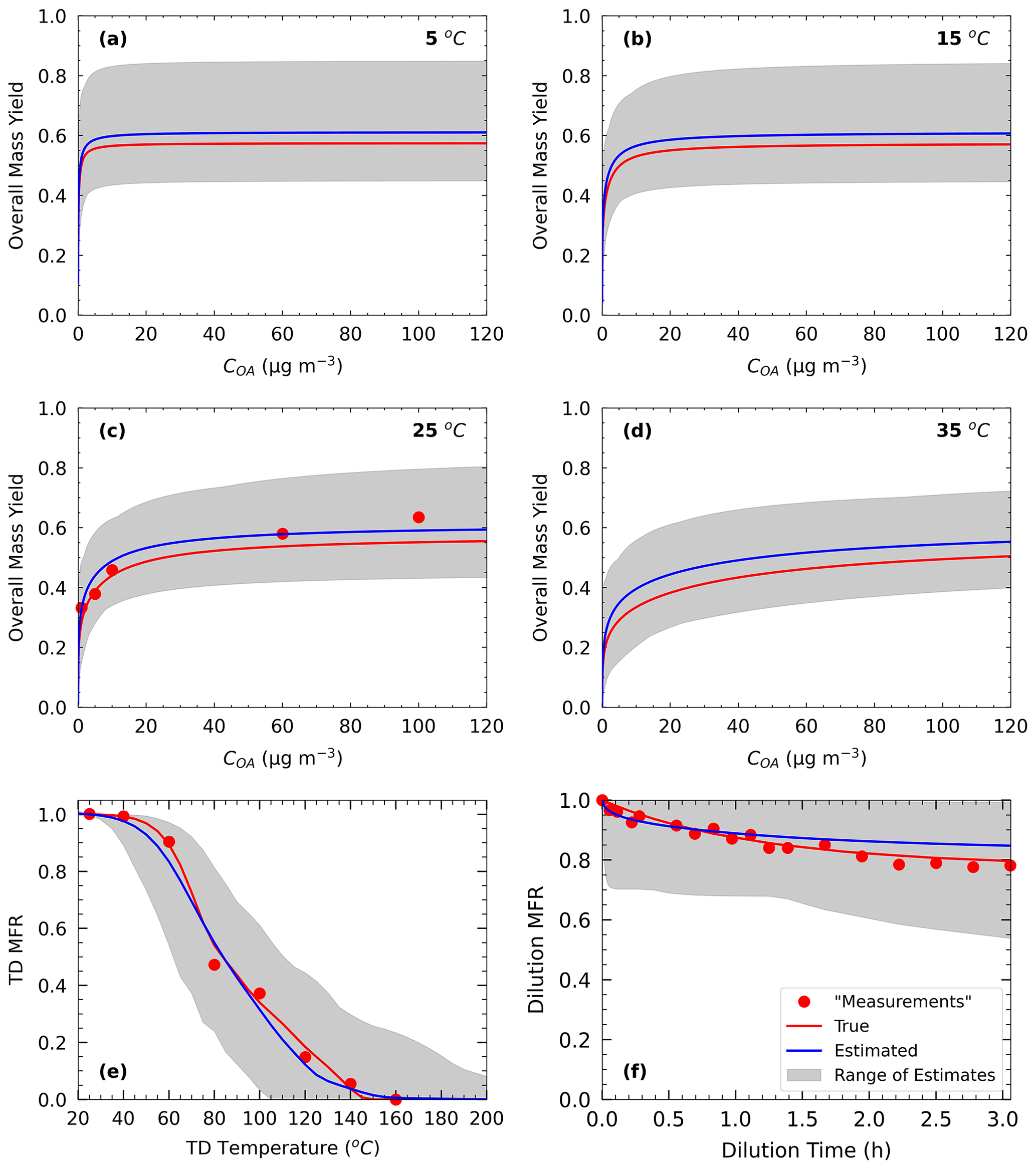
Figure 3 Measurements of Test C1 in Experiment C (red dots) and true (red line) and estimated (blue line) yields at (a) 5 ^∘C, (b) 15 ^∘C, (c) 25 ^∘C, and (d) 35 ^∘C, with (e) TD (thermogram) and (f) dilution (areogram) values. The grey area shows the range of good solutions.

For Experiment C, the true values were based on the parametrization of the SOA formed during α-humulene ozonolysis by Sippial et al. (2023). The authors measured high SOA yields for α-humulene in the main smog chamber (∼ 70 % at 60 µg m⁻³), and their corresponding thermogram suggested that the SOA particles fully evaporated at 150 ^∘C, while the areogram showed modest (20 %) evaporation in the dilution chamber after 3 h. A four-volatility-bin set with saturation concentrations ranging from 10⁻² to 10 µg m⁻³ was used in that study to fit the measurements. The stoichiometric coefficients of the three least volatile bins (10⁻², 10⁻¹, and 1 µg m⁻³) were around 0.1 and of the most volatile (10 µg m⁻³) 0.25. The vaporization enthalpy was 115 kJ mol⁻¹, and the accommodation coefficient was 0.01 (Table S1). We assumed five yield measurements in the SOA concentration range of 1 to 100 µg m⁻³ with yield values as high as 65 % at 100 µg m⁻³ (Fig. 3). The corresponding thermogram consisted of 10 data points, and the particles fully evaporated at TD temperatures higher than 150 ^∘C. The areogram consisted of 17 data points, and only 20 % of the SOA evaporated in the dilution chamber.

4.2 Parameter estimation for Experiments A, B, and C

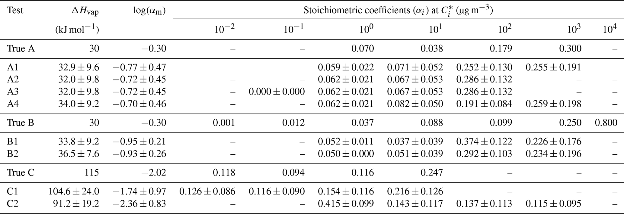
We explored the performance of the algorithm for different choices of the number of volatility bins, the range of saturation concentrations, and the range of SOA mass concentration in the yield measurements. For each test, the true and the estimated properties are summarized in Table 1.

Table 1 True and estimated volatility distribution of the products for eight different tests. The uncertainty in the estimates (±σ) is also included.

We evaluated the performance of our parameter estimation algorithm, comparing its predictions against both the measurements and the “truth” defined as the predictions of the original parametrization. In both comparisons, mean normalized error (MNE) (Emery et al., 2017) was used as the evaluation metric because it has a simpler physical meaning than NMSE.

For the evaluation against the measurements, MNE_M was defined as follows:

$$\begin{array}{}\text{(16)}& {\mathrm{MNE}}_{\mathrm{M}}={\displaystyle \frac{\mathrm{100}}{N_{\mathrm{O}}}}\sum _{i=\mathrm{1}}^{N_{\mathrm{O}}}{\displaystyle \frac{\left|{\mathrm{EST}}_i-O_i\right|}{O_i}},\end{array}$$

where EST_i is estimated by the algorithm value and corresponds to a specific measured point O_i.

For the evaluation against the truth, which includes conditions (e.g., temperatures or concentrations) for which there are no available measurements, MNE_T was defined as follows:

$$\begin{array}{}\text{(17)}& {\mathrm{MNE}}_{\mathrm{T}}={\displaystyle \frac{\mathrm{100}}{N_{\mathrm{d}}}}\sum _{j=\mathrm{1}}^{N_{\mathrm{d}}}{\displaystyle \frac{\left|{\mathrm{EST}}_j-{\mathrm{TR}}_j\right|}{{\mathrm{TR}}_j}},\end{array}$$

where EST and TR are the estimated and the true values respectively. N_d is the total number of data points included in calculations and depends on the selected discretization of the corresponding dependent variable (e.g., SOA concentration, TD temperature, and dilution time). We used a linear discretization for the SOA concentrations (from 0.01 to 50 µg m⁻³ with a step of 0.01) and the TD temperatures (20 to 200 ^∘C with a step of 5 ^∘C but excluding zero-MFR values to avoid the division by zero). For the dilution time, the sampling time step was not constant. We used a higher resolution for the first 0.5 h (step of 2 min), in which the evaporation is usually faster, and a lower resolution afterwards (step of 10 min).

Finally, we used the average relative standard deviation (ARSD) as a metric to quantify the uncertainty in the estimates (range of good solutions) using the same discretization as in the MNE_T metric. The ARSD is given by

$$\begin{array}{}\text{(18)}& \mathrm{ARSD}={\displaystyle \frac{\mathrm{100}}{N_{\mathrm{d}}}}\sum _{j=\mathrm{1}}^{N_{\mathrm{d}}}{\displaystyle \frac{{\mathit{\sigma }}_j}{{\mathrm{EST}}_j}},\end{array}$$

where σ_j is the standard deviation for data point j.

4.2.1 Parameter estimation for Experiment A

In Test A1, we applied the algorithm in the same range of saturation concentrations and with the same number of volatility bins as those used to produce the experimental data. The upper bin (10³ µg m⁻³) exceeded the maximum SOA concentration (40 µg m⁻³) in the measurement range by 1 order of magnitude.

Figure 1 depicts the estimated and the range of the ensemble of best solutions for the three types of measurement for Test A1. There were 148 good solutions under the 5 % threshold out of the 126 120 simulations (Table S3). The density distribution of the solutions is depicted in Fig. S1. The performance of the model for the yields at 25 ^∘C was quite encouraging with a small tendency of overprediction for SOA higher than 10 µg m⁻³. The MNE_M of the model for the SOA yield measurements (given by Eq. 16) was equal to 25 % (Table 2). The corresponding discrepancy between the true parametrization and the measurements (due to the measurement error that we introduced) was 21.2 % (Table 2). This indicates that a significant part of the algorithm error can be explained by the uncertainty introduced into the measurements.

Table 2 The mean normalized error (MNE) between the measurements and true values and between the measurements and the model-estimated values for the different tests.

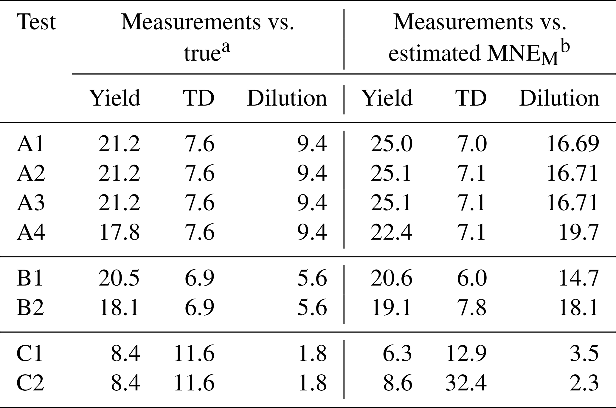
^a Calculated by $\frac{\mathrm{100}}{N_{\mathrm{O}}}\sum _{i=\mathrm{1}}^{N_{\mathrm{O}}}\frac{\left|O_i-{\mathrm{TR}}_i\right|}{O_i}$. ^b Calculated by Eq. (16).

Our algorithm can be used to calculate the SOA yield at different concentrations and temperatures. The yields were calculated in the atmospherically relevant range of 0–50 µg m⁻³ SOA concentration and at four temperatures (5, 15, 25, and 35 ^∘C) using the true parameter values and the estimated parameters of Test A1 (Fig. 1a–d). At 25 ^∘C (Fig. 1c), the estimated yield curve is in good agreement with the true yield curve for SOA concentrations lower than 6 µg m⁻³ (error of 8 % at 6 µg m⁻³), but the discrepancies increase at higher concentrations (error of 23 % at 50 µg m⁻³). The average MNE_T error between the true parametrization and the estimated values (given by Eq. 17) was equal to 17.3 % for yields at 25 ^∘C (Table 3). The uncertainties, as expected, are larger at lower temperatures. However, the MNE_T error (estimated yields compared to the true value) remains less than 25 % (Table 3) even at 5 ^∘C, quite far from the measurement temperature. Both MNE_T and MNE_M were quite close to the introduced experimental error. Their difference can be explained by both the noise introduced to the measurements that affects MNE_M and the higher number of points used to calculate MNE_T.

Table 3 The mean normalized error between the true and estimated values (MNE_T) for the different tests.

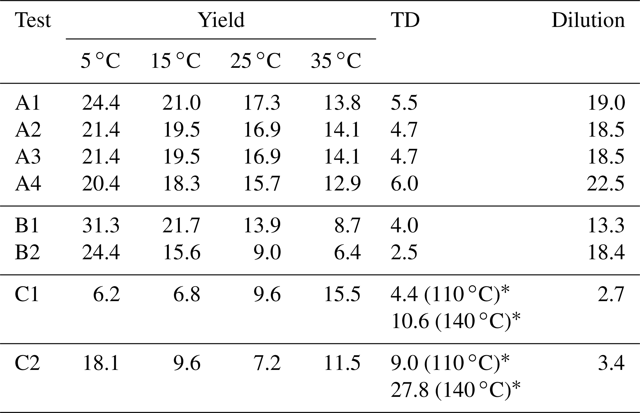
^∗ The errors for TD were calculated up to the denoted temperature in the parentheses.

The SOA model used in this work assumes that the stoichiometric coefficients (α_i) are temperature independent. Therefore, processes which are expected to be temperature dependent, such as formation of highly oxygenated organic molecules (HOMs) and oligomerization (Quéléver et al., 2019; Gao et al., 2022), are not described by our algorithm.

The algorithm provides a range of good estimates in addition to the best estimate. The range can be defined by the lower and upper SOA yield limits of the ensemble of the good solutions at each point. At 25 ^∘C, the yield range increased, as expected, at higher concentrations (yield range of 0.05 at 1 µg m⁻³ to 0.17 at 50 µg m⁻³). The average relative standard deviation (ARSD of the estimated yields defined by Eq. 18) was equal to 26 % (Table 4) for the 25 ^∘C case. For the rest of the temperatures, the ARSD increased for the lower temperatures, ranging from 24 % at 35 ^∘C to 35 % at 5 ^∘C (Table 4) and including in all cases the true solution.

Table 4 The average relative standard deviation (ARSD) for the different tests.

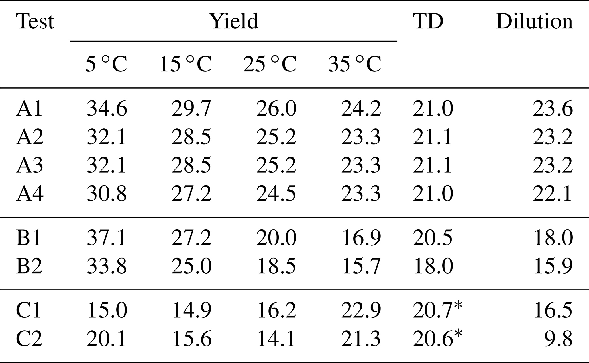
^∗ The ARSD for the TD MFR values were calculated in the 20–120 ^∘C temperature range.

For the TD (Fig. 1e), the model reproduced well the correspondent thermogram with low errors compared to the measurements with an error MNE_M of 7 % (Table 2). The error MNE_T compared to the true values was 5.5 % (Table 3). The error in the TD measurements compared to the true values was equal to 7.6 % (Table 2). Therefore, the error in the proposed algorithm is quite similar to the experimental error. The error introduced into the measurements was transferred, as expected, to the error metrics of the algorithm.

For the isothermal dilution (Fig. 1f), the algorithm did reasonably well for the first 30 min and then the evaporation was slightly underpredicted, leading to an error in MNE_M of 16.7 % (Table 2). This MNE_M value was roughly 2 times higher than the corresponding error between the dilution measurements and the true parametrization (Table 2). The error between the estimated and the true values of MNE_T was 19 %. The ARSD of 24 % (Table 4) was sufficient to include the true solution.

The estimated volatility distribution of the products and the effective vaporization enthalpy and accommodation coefficient using the three types of measurement can be seen in Fig. 4 and Table 1. The estimated volatility distribution of the products was in good agreement with the true values (α_i absolute difference of 0.01 at 1 µg m⁻³, 0.03 at 10 µg m⁻³, 0.07 at 10² µg m⁻³, and 0.04 at 10³ µg m⁻³), and the estimated uncertainties contained the correct values. There is a large uncertainty range for the two higher volatility bins (standard deviation higher than 0.13), indicating that yield values at higher SOA concentrations would be needed to better constrain these volatility bins. The relative error in the estimated ΔH_vap is 10 %. The estimated accommodation coefficient was 0.17 compared to a true value of 0.5. The estimated uncertainty for the effective accommodation was almost 1 order of magnitude higher (from 0.06 to 0.51), indicating the difficulty of constraining this parameter when it is close to unity and thus the resistances to mass transfer are small.

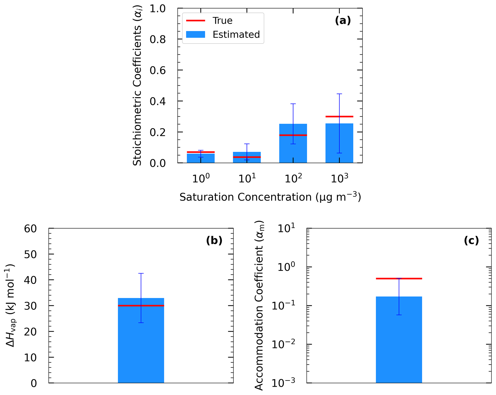
Figure 4 Estimated (bars) and true (red lines) parameter values of Experiment A in Test A1 combining yield, TD, and isothermal dilution measurements for (a) the volatility distribution of the products, (b) ΔH_vap, and (c) α_m. The error bars represent the uncertainty in the estimated values.

4.2.2 Parameter estimation for Experiment B

In this section, we analyze the pseudo-experimental data of Experiment B, which were obtained from the parametrization of the same smog chamber results used in Experiment A but with more components and a much wider range of volatilities including LVOCs, SVOCs, and IVOCs (10⁻²–10⁴ µg m⁻³). In Test B1, the algorithm was applied using a four-bin VBS with saturation concentrations ranging from 1 to 10³ µg m⁻³. In this test, we attempted to model the behavior of the system with a narrower volatility range than the real one. The upper limit of the saturation concentration range that we tested did not exceed 10³ µg m⁻³ because Experiment B took place at moderate SOA concentration levels (up to 40 µg m⁻³), which means that it is practically impossible to constrain the 10⁴ µg m⁻³ or higher volatile bins. Figure 2 shows the results of the fitting for the three types of measurement in this experiment. There were 82 good solutions under the 5 % threshold out of 126 120 simulations (Table S3), and the density of the solutions are shown in Fig. S2. At 25 ^∘C, the model performance for the yields is encouraging (MNE_M = 20.6 %). This is again pretty close to the measurement error (20.5 %). By comparing the estimated and the true yield curves at 25 ^∘C, the error MNE_T is now 14 %. The error increases to 31 % at 5 ^∘C, far from the available measurements. This is also reflected in the increase in the uncertainty in our estimates with the ARSD increasing from 17 % at 35 ^∘C to 37 % at 5 ^∘C (Table 4). Once more the uncertainty range estimated by the algorithm includes the true values.

Both measured and true thermograms were well captured by the best estimate (MNE_M of 6 % and MNE_T of 4 %) with an uncertainty ARSD of 20.5 %. The evaporation in the dilution chamber was a little underestimated for the first 2 h, but then it was slightly overpredicted. The MNE_T for the areogram was 13.3 %, and the true values were included within the range of the estimates (ARSD of 18 %).

Figure 5 shows the results of Test B1 for the volatility distribution of the products. The true stoichiometric coefficient for the 1 µg m⁻³ bin was overestimated by 0.01 by the algorithm. This overestimation actually corresponds to the total material of the 10⁻² and 10⁻¹ µg m⁻³ bins of the true system. This indicates that the algorithm places the material of the two lowest bins that are not part of the solution in the bin with the lower volatility. For the 10 and 10² µg m⁻³ bins, the relative errors between the estimated and true results were 58 % and 277 % respectively (Table S4), while for the 10³ µg m⁻³ bin, the relative error was 10 %. The ΔH_vap was predicted accurately (error of only 4 %), while α_m was underpredicted (0.1 instead of 0.5). The model compensates for the missing volatility bins by increasing the material in the 10² µg m⁻³ bin and by decreasing the accommodation coefficient.

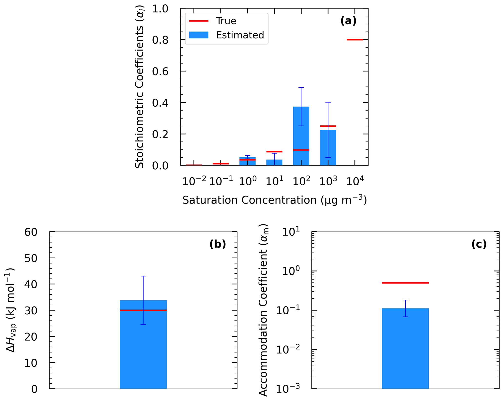
Figure 5 Estimated (bars) and true (red lines) parameter values of Experiment B in Test B1 combining yield, TD, and isothermal dilution measurements for (a) the volatility distribution of the products, (b) ΔH_vap, and (c) α_m. The error bars represent the uncertainty in the estimated values.

The results of Test B1 suggest that the mismatch between the actual SOA volatility distribution and the range used for the fits can introduce significant errors into the retrieved distribution for individual volatility bins. However, despite these problems, the yields predicted by the derived parametrizations have a much lower error than the volatility distribution. This is a valuable insight for the strengths and weaknesses of this and other similar SOA parameter estimation algorithms.

4.2.3 Parameter estimation for Experiment C

In Test C1, we obtained the best fits for the pseudo-measurements of Experiment C by applying the algorithm in the same range of saturation concentrations and with the same number of volatility bins (four volatility bins in the 10⁻²–10¹ µg m⁻³ saturation concentration range) as the true volatility distribution.

Figure 3 shows the results of the fitting for the three types of measurement. There were 3479 good solutions under the 5 % threshold out of the 126 120 simulations (Table S3). The density distribution of the solutions is shown in Fig. S3. The best estimate for the SOA yields at 25 ^∘C was in a good agreement with the measurements (MNE_M = 6.3 %) and the true values (MNE_T = 9.6 %). For the rest of the temperatures, there was a decreasing trend of the error as the temperature decreased varying from 15.5 % at 35 ^∘C to 6.2 % at 5 ^∘C. A similar decreasing trend was observed for the uncertainty ARSD of the estimates, which varied from 23 % at 35 ^∘C to 15 % at 5 ^∘C. This behavior is the opposite of what we observed in the previous tests, in which both errors and uncertainties increased at lower temperatures. However, the changes in both the error and the uncertainty are small (change of around 7 % between the upper and lower temperature for both metrics), indicating that this system is less temperature-sensitive in this temperature range than the previous ones.

The performance of the algorithm was satisfactory compared to the TD measurements (MNE_M = 12.9 %). The corresponding error in the algorithm for the true values (MNE_T) was 4.4 % for temperatures up to 110 ^∘C and equal to 10.6 % for the lower values at higher temperatures. According to Fig. 3, the evaporation due to dilution was initially overestimated for the first 30 min but then underestimated (highest MFR discrepancy of 0.05), and there is a high uncertainty range of the corresponding estimates (MFR range of 0.46 at 3 h). However, the low dilution values resulted in low relative errors (MNE_M of 3.5 % and MNE_T of 2.7 %).

Figure 6 shows that the highest relative errors were calculated for the 10⁻¹ and 10⁰ µg m⁻³ bins (23 % and 33 % respectively), and smaller relative errors were calculated for the other two bins (less than 13 %). The uncertainties were almost of the same magnitude for all bins with standard deviations ranging from 0.09 to 0.13. The performance of the model was good for ΔH_vap (relative error of 7 %) but with high uncertainty for α_m.

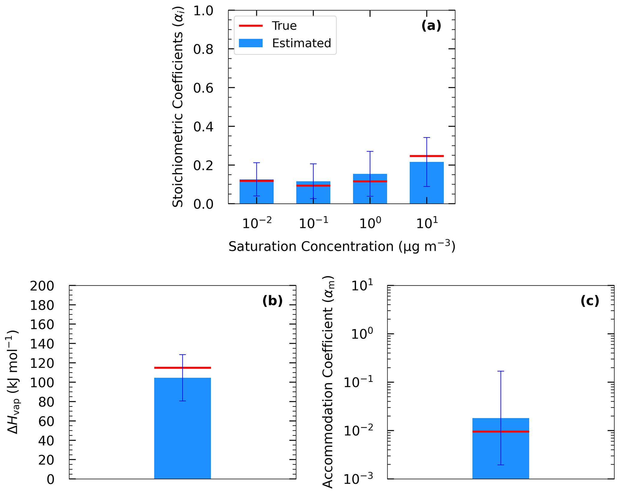
Figure 6 Estimated (bars) and true (red lines) parameter values of Experiment C in Test C1 combining yield, TD, and isothermal dilution measurements for (a) the volatility distribution of the products, (b) ΔH_vap, and (c) α_m. The error bars represent the uncertainty in the estimated values.

4.3 Effect of the volatility range

In this section, we explore the performance of the algorithm for different choices of the number of volatility bins and the range of saturation concentrations. The analysis of the results of Test B1 has already quantified the effects of using a narrower volatility distribution in the parameter estimation algorithm than the one of the investigated SOA system. Additional sensitivity tests are performed here for all cases.

In Test A2, we used three volatility bins covering the 1–10² µg m⁻³ saturation concentration range instead of the four bins used in Test A1. The narrower assumed volatility range had a very small effect on the estimated yields at all temperatures (Table 3 and Fig. S4) compared to Test A1. The change in MNE_T ranged from 3 % at 5 ^∘C to 0.3 % at 35 ^∘C. Minor changes were detected in the predicted thermogram (change of 0.8 %) and areogram (change of 0.5 %) as well. The uncertainty in the yield estimates increased by less than 2.5 % at all temperatures. The estimated volatility distribution of the SOA products of Test A2 changed by less than 5 % in the two lower bins. The material in the 10² µg m⁻³ bin increased by 15 % to account for the SOA of higher volatility that could not be included otherwise in the estimated distribution. The estimated ΔH_vap was in this case 32 kJ mol⁻¹ (2.7 % decrease), and α_m decreased by 12 % with respect to Test A1.

In Test A3, we shifted the assumed four-bin volatility distribution by 1 order of magnitude to lower values (from 1–1000 µg m⁻³ in Test A1 to 0.1–100 µg m⁻³ in Test A3). In this case, the algorithm distributed exactly the same material to the 1, 10, and 100 µg m⁻³ volatility bins as in Test A2, and it predicted correctly zero SOA in the 0.1 µg m⁻³ bin (Table 1). The ΔH_vap and α_m estimated values were also unchanged with respect to Test A2. This, in turn, led to the same estimated yields at different temperatures (no change in the error between the two tests).

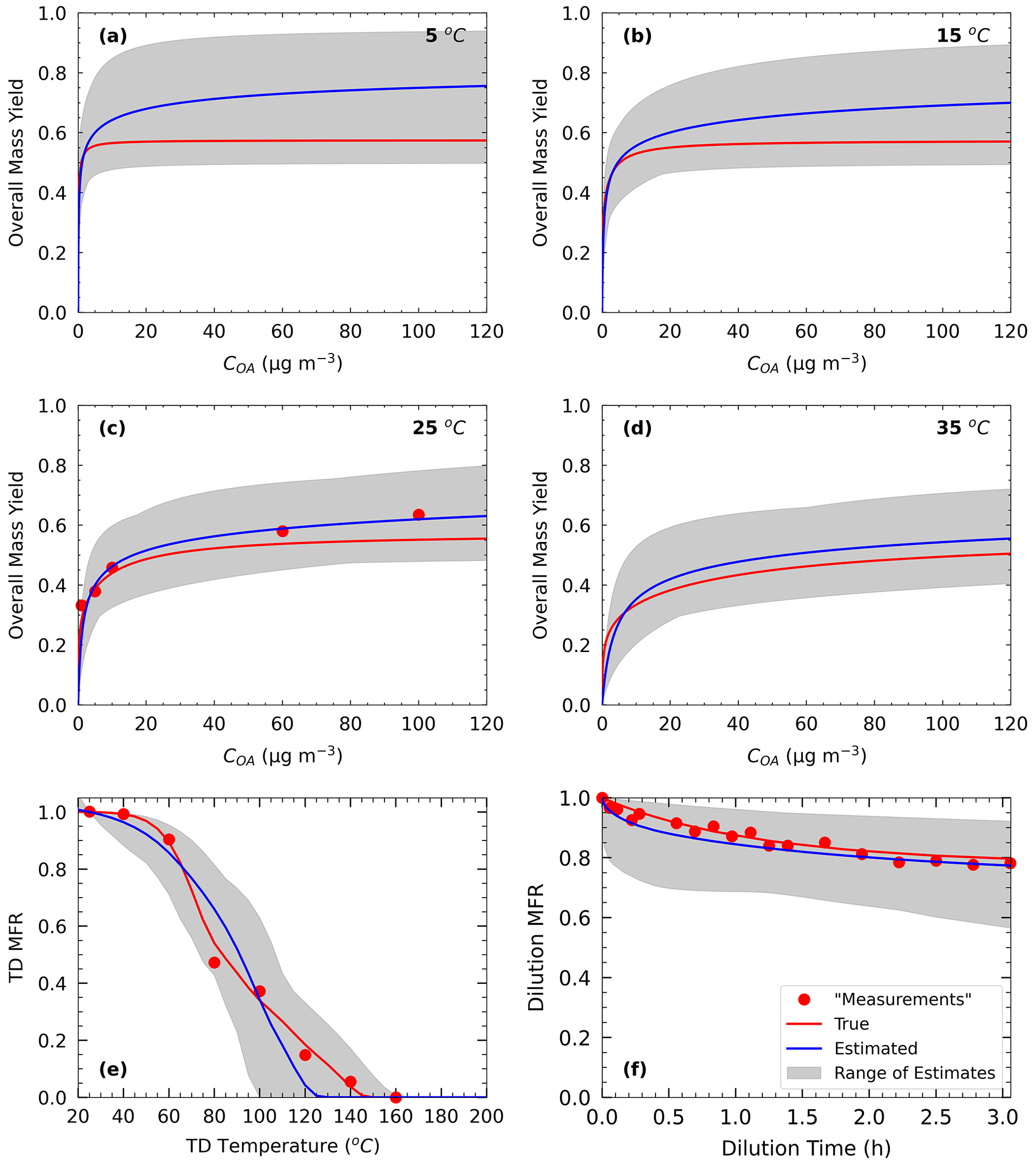
Figure 7 Yields calculated using the true parameters of Experiment C (red line) and estimated (blue line) using the parameters of Test C2 for the following temperatures: (a) 5 ^∘C, (b) 15 ^∘C, (c) 25 ^∘C, and (d) 35 ^∘C. Also shown are the (e) thermogram and (f) areogram. The grey area shows the range of good solutions obtained by our algorithm.

In Test C2, we applied the algorithm against the Experiment C measurements using a four-volatility-bin system in the 1-to-10³ µg m⁻³ range, which is 2 orders of magnitude higher than the actual range of the true values. Figure 7 shows the results of the fitting for the three types of measurement. Despite the significant mismatch of the volatility distributions, MNE_M increased by only 2.3 % for the estimated SOA yields. The error for the TD measurements increased by 20 %, while it actually decreased a little (1.2 %) for the dilution data. The errors compared to the true values increased by less than 3 % for the temperature range 15–35 ^∘C, while it increased by 12 % at 5 ^∘C. These results suggest that in this case the estimated yields are quite robust to the assumed volatility range. The major effect of the mismatch in volatility ranges was evident in the predicted thermogram with overestimation of the MFR for the 60–120 ^∘C temperature range and underprediction at higher temperatures. The increase in MNE_T for the TD MFR was 17.2 % (Table 3). The change in the predicted areogram was marginal and led to a small increase in MNE_T (error increase by 0.7 %) (Table 3). The algorithm not only underestimated again α_m (0.004 instead of 0.01) but also recognized the high uncertainty in the corresponding estimate. The algorithm distributed significant material to the 1 µg m⁻³ bin (3.6 times higher than the actual amount) in an effort to account for the absence of the 10⁻² and 10⁻¹ µg m⁻³ bins. The ΔH_vap was underestimated with an error of 21 %.

The results of the above tests indicate that a mismatch between the true and assumed volatility ranges of the SOA increases in general the estimation error but the increase is small to modest. This is reassuring for the robustness of the proposed algorithm.

4.4 Effect of measurements at high SOA levels

During the last decade there has been a significant shift of the performed SOA smog chamber towards lower SOA concentrations. This is needed to increase the accuracy at ambient concentration levels. The high-SOA-concentration experiments that once represented the majority of performed experiments are becoming increasingly rare. In this subsection we examine the value of these high-concentration experiments for the estimation of SOA yields under ambient conditions.

To examine the effect of measurements at SOA levels much higher than the atmospheric ones, we included an extra yield measurement at 200 µg m⁻³ in the yield data of Experiments A and B. In Test A4 and B2, we applied the algorithm once again against the three types of measurement by using a four-volatility-bin system with saturation concentrations ranging from 1 to 10³ µg m⁻³.

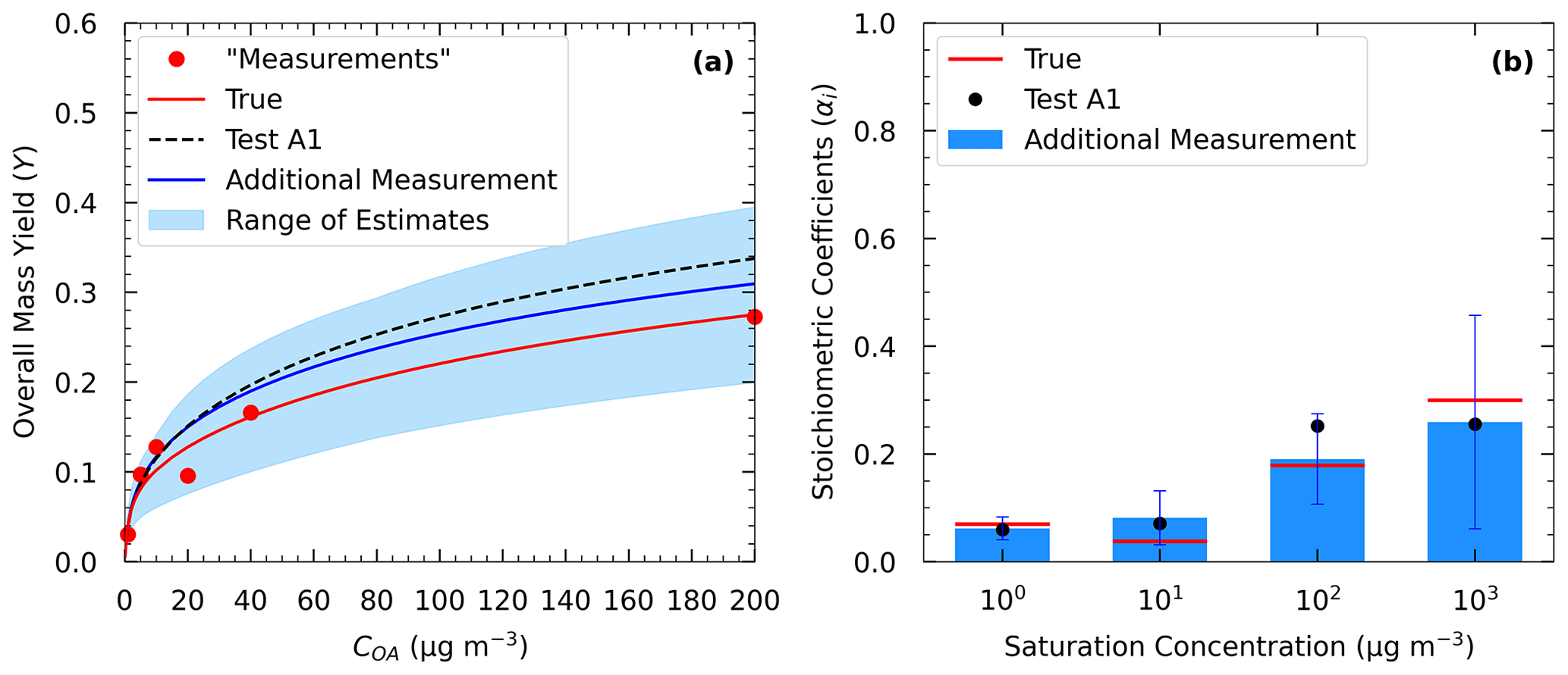
Figure 8 (a) True (red line) and estimated (blue line) yields in Test A4 and the measurements of Experiment A (red dots) including an additional yield measurement at 200 µg m⁻³. The dashed black line corresponds to the estimated yields in Test A1. (b) Estimated volatility distribution of the products (bars) of Test A4 and the true (red lines) parameter values. The black dots correspond to the estimated volatility distribution of the products in Test A1.

In Test A4, the additional experiment at high SOA concentration led to an MNE_T of 15.7 % for the yields at 25 ^∘C (Table 3 and Fig. S5), which is lower by 1.6 % than that without this experiment in Test A1. The improvement was more significant at lower temperatures; e.g., MNE_T at 5 ^∘C was reduced from 24.4 % to 20.4 %. The reduction in the ARSD for the SOA yields ranged from 3.8 % at 5 ^∘C to 0.9 % at 35 ^∘C (Table 4). Figure 8 depicts the results of the model for the yields and the volatility distribution of the products for Test A4. The accuracy of the predicted volatility distribution increased especially for the higher-volatility material. For example, the error for the 10² µg m⁻³ bin was reduced from 41 % in Test A1 to 6 % in this case (Table S3). Minor changes in the errors were detected for ΔH_vap and α_m between the two tests (3 % increase and 6 % decrease respectively).

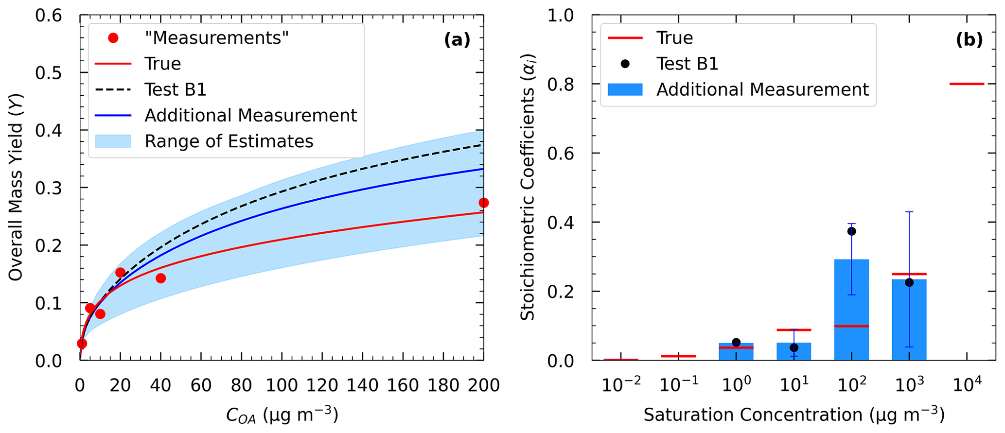
Figure 9 (a) Estimated yields (blue line) in Test B2 and measurements of Experiment B (red dots) including an additional yield measurement at 200 µg m⁻³. The dashed black line corresponds to the estimated yields in Test B1. (b) Estimated volatility distribution of the products (bars) of Test B2 and the true (red lines) parameter values. The black dots correspond to the estimated volatility distribution of the products in Test B1.

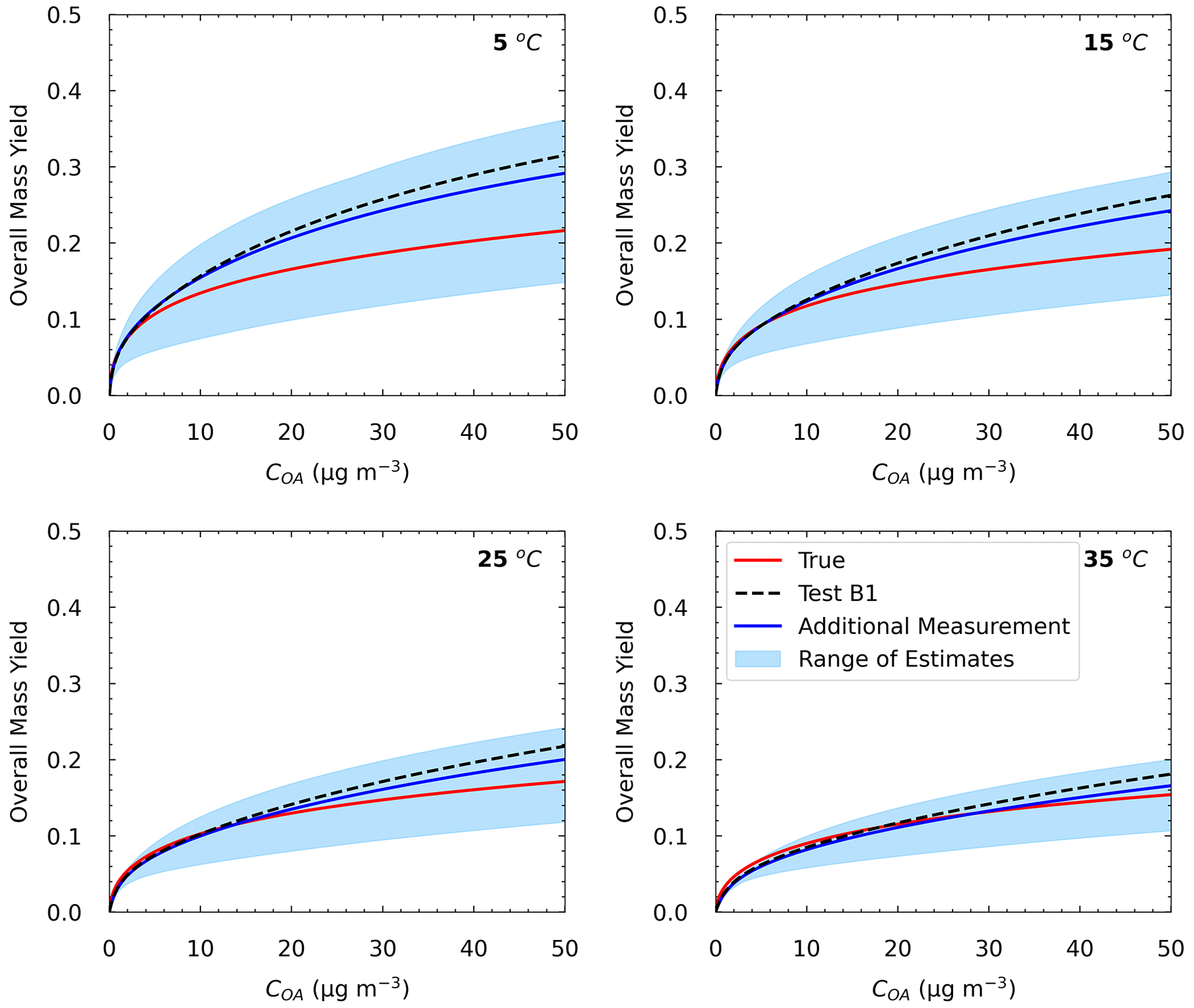
Figure 10 Yields calculated using the true parameters of Experiment B (red line) and the estimated (blue line) using the parameters of Test B2 for the following temperatures: 5, 15, 25, and 35 ^∘C. The blue area shows the range of good solutions obtained by our algorithm. The dashed black line corresponds to the estimated yields in Test B1.

Similarly to Test A4, in Test B2 we added a yield measurement at 200 µg m⁻³ in the Experiment B set of measurements. Figure 9 depicts the results of the model for the SOA yields at 25 ^∘C and the estimated volatility distribution of the products. The use of the additional data point led to a reduction in the MNE_T from 13.9 % in Test B1 to 9 % in Test B2 at 25 ^∘C (Table 3). Similar reductions in the MNE_T were observed for the other temperatures, with the highest one observed at 5 ^∘C (lower error by 7 %) (Fig. 10). The reduction in the ARSD for the estimated yields ranged from 3.3 % at 5 ^∘C to 1.2 % at 35 ^∘C (Table 4). Minor changes were observed for the estimated thermogram (Fig. S6) (change in the MNE_T of 1.5 %) and the uncertainty in the estimates (change in the ARSD of 2.5 %). The error in the estimated areogram was also small, but in this case the error increased by 5 %. The additional data point helped decrease the errors for the estimated mass of the more volatile SOA products (Fig. 9) and especially for the 10² µg m⁻³ bin. The ΔH_vap and α_m estimated values were only slightly affected by the additional measurement.

By comparing the results of Tests B1 and B2 with Case A, one would expect the retrieved volatility distribution of the products to be quite similar. The differences present are due to a large extent to the different random experimental errors introduced into the two sets of measurements for Experiments A and B. A second reason for the differences is that parametrizations of the two “experiments” by Pathak et al. (2007b), even if they were derived from the same smog chamber experiments, have some differences. As a result, the true yields, thermogram, and areogram in Cases A and B are not exactly the same (Figs. 1 and 2).

These results suggest that an additional yield measurement at high SOA levels can lead to a substantial reduction in the error for the estimated yields at low temperatures (Fig. 10) and also a better estimation of the SOA products with higher volatility (10² and 10³ µg m⁻³). These products may contribute little to the SOA concentration at 25 ^∘C, but their reactions (aging) could lead to significant additional SOA in later stages.

4.5 Significance of each type of measurement for the parametrization

To quantify the effect of each type of measurement on the parameter estimation and their subsequent effect on the estimated SOA yields, we repeated Tests A1, B1, and C1 withholding one set of measurements. More specifically, we provided the algorithm with the following combination of measurements: TD and isothermal dilution, SOA yields and isothermal dilution, and finally SOA yields and TD.

The use of only the TD and isothermal dilution data corresponds for all practical purposes to the previous algorithm of Karnezi et al. (2014), which was the starting point of this work. In Test A1, the absence of the yield measurements led to a significant deterioration of the ability of the algorithm to estimate SOA yields at all temperatures and concentrations (Fig. S7). The SOA yield error in the algorithm in the 5–35 ^∘C temperature range increased from 14 %–24 % (when all measurements are provided) to approximately 100 % (Table S5). The corresponding uncertainty range also increased by a factor of 4–6 (Table S6). Similar results were obtained in the other tests.

Figure S8 shows the volatility distribution of the products, ΔH_vap, and α_m in Test A1. High discrepancies and uncertainties were observed for the estimated stoichiometric coefficients (α_i), with an increase in the relative error by a factor of 3–4 for the 1 and 10 µg m⁻³ bins (Table S7) compared to the case when all three types of measurement are used.

Figures S9 and S10 show the results of the algorithm for Test A1 when only the SOA yields and isothermal dilution measurements are provided as inputs to the algorithm. In this case the algorithm cannot constrain well the ΔH_vap (relative error of almost 270 % with respect to the true value) as a result of the missing TD measurements. This led to a significant increase in MNE_T for the estimated yields when moving far from the temperature of the measurements (MNE of 65 % at 15 ^∘C and 122 % at 5 ^∘C).

Figures S11 and S12 show the results of the algorithm for Test A1 when only yield and TD measurements are provided as inputs. In this case, there was a significant reduction in the error for ΔH_vap with respect to the previous case (from 270 % to 50 %), but it was still much higher than the 10 % error when all three types of measurement were used. This led to better agreement between the true and estimated yields at lower temperatures (MNE_T of 23 % and ARSD of 44 %).

When comparing TD–dilution, yield–dilution, and yield–TD results, the yield–TD combination gave the best results out of the three pairs. The isothermal dilution measurements are the least valuable of the three because only a relatively small fraction of the SOA evaporates and therefore the information provided is relatively limited and focuses on the more volatile components of the particles. Also, TD measurements are important to constrain ΔH_vap well and allow the more accurate extrapolation of the results to other temperatures. However, our results suggest that the combination of the three types of measurement leads to a major improvement over either the TD–dilution approach or the yield–TD approach.

4.6 Sensitivity to the upper limit of the sum of product yields

The maximum sum of the VBS product yields is one of the parameters that the user of the algorithm chooses. In the analysis so far, a value of 1 has been selected to reduce the computational cost of the algorithm. Selected tests were repeated using a maximum sum of 2 to quantify the effects of this choice on the estimated parameters and more importantly on the SOA yields predicted by the parametrization. For a four-product system, there are 9191 product yield combinations, and considering the discretization of ΔH_vap and α_m, this leads to a total of 367 120 simulations (Table S3).

The increase in the upper limit of the sum of the yields led to an increase in the good solutions in Tests A1, A4, B1, B2, and C2. The additional solutions had different yields mostly in the 10³ µg m⁻³ bin. This led to an increase in the mass yield of this bin by 37 % in Test A1, 47 % in Test B1, and 29 % in Test C2 (Table S8). The uncertainties were even higher, showing once again the difficulty of constraining the IVOC range where there are no SOA measurements at very high SOA concentrations. The new parametrizations had a minor effect on the estimated yields at different temperatures with maximum change in the MNE_T found at 5 ^∘C (change of 1.8 % in Test A1 and 1.2 % in Test B2) and much smaller change otherwise (Table S9). Therefore, the use of the higher upper limit has an effect on the estimate of the 10³ µg m⁻³ bin, which is quite uncertain in all cases, but has a minor effect on the predicted SOA yields at ambient conditions.

5 Conclusions

An algorithm was developed to estimate VBS parameters for SOA formation combining yield measurements from atmospheric simulation chambers with thermodenuder and isothermal dilution measurement chambers. An additional feature of this approach is that the algorithm estimates the uncertainty in the predicted SOA yields for different SOA concentrations and temperatures, assisting in this way in the design of future experiments.

The algorithm was evaluated against pseudo-experimental data for SOA systems with known properties. The algorithm performed quite well at reproducing the SOA yields at atmospherically relevant concentrations and temperatures with errors less than 20 % for practically all cases. This was the case even at temperatures as low as 5 ^∘C and also when the volatility range used for the parameter estimation was narrower than that of the simulated SOA system. One should note that this error was quite similar in most cases to the experimental error assumed in the construction of the measurement datasets.

The errors in the retrieved SOA volatility distributions were in general higher than those of the SOA yields. This is due to a large extent to the existence of multiple solutions that can result in similar yields. The accuracy of the estimated mass fractions of the more volatile SOA components improved with an additional yield measurement at high SOA levels (e.g., at 200 µg m⁻³). The addition of this measurement also improved the estimated yields at low temperatures. This therefore suggests that data points at high SOA concentrations should also be obtained experimentally, together with the data points at atmospherically relevant atmospheric SOA levels.

In all cases the algorithm results in good estimates of the effective evaporation enthalpy. On the other hand, the estimates of the effective accommodation coefficient are usually quite uncertain. The effect of the mass accommodation coefficient on the measured quantities is relatively small compared to the other parameters (volatility distribution, effective evaporation enthalpy), making it difficult to constrain. This conclusion is consistent with the results of Karnezi et al. (2014). The addition of the SOA yields to the inputs does not make much of a difference because these are not affected by the accommodation coefficient.

The approach combining yield, TD (thermograms), and isothermal dilution (areograms) measurements is recommended for future parametrizations of SOA formation. The use of the results of these experiments that have been designed for the measurement of SOA yields in other applications (e.g., new particle formation) should be performed with caution. Our results indicate that the derived parametrizations are able to predict the SOA yields under different atmospheric conditions with errors of around 20 % or less, but the derived volatility distributions can be quite uncertain. These uncertainties are higher for the tails of the distribution (the low-volatility and the intermediate-volatility organic compounds). Different experiments should probably be performed for the derivation of the VBS distribution if for example one is interested in new particle formation and therefore the low-volatility organics focusing on low SOA concentration levels and the least volatile SOA components.