In-orbit cross-calibration of millimeter conically scanning spaceborne radars

The planned and potential introduction in global satellite observing systems of conically scanning Ka- and W-band atmospheric radars (e.g., the radars in the Tomorrow.IO constellation, https://www.tomorrow.io/space/, last access: 1 June 2022, and the Wivern (WInd VElocity Radar Nephoscope) radar, https://www.wivern.polito.it, last access: 1 July 2022) calls for the development of methodologies for calibrating and cross-calibrating these systems. Traditional calibration techniques pointing at the sea surface at about 11^∘ incidence angle are in fact unfeasible for such fast rotating systems.

This study proposes a cross-calibration method for conically scanning spaceborne radars based on ice cloud reflectivity probability distribution functions (PDFs) provided by reference radars like the Global Precipitation Measurement (GPM) Ka-band radar or the W-band radars planned for the ESA-JAXA EarthCARE or for the NASA Atmosphere Observing System missions. In order to establish the accuracy of the methodology, radar antenna boresight positions are propagated based on four configurations of expected satellite orbits so that the ground-track intersections can be calculated for different intersection criteria, defined by cross-over instrument footprints within a certain time and a given distance. The climatology of the calibrating clouds, derived from the W-band CloudSat and Ka-band GPM reflectivity records, can be used to compute the number and the spatial distribution of calibration points. Finally, the mean number of days required to achieve a given calibration accuracy is computed based on the number of calibration points needed to distinguish a biased reflectivity PDF from the sampling-induced noisiness of the reflectivity PDF itself.

Findings demonstrate that it will be possible to cross-calibrate, within 1 dB, a Ka-band (W-band) conically scanning radar like that envisaged for the Tomorrow.io constellation (Wivern mission) every few days (a week). Such uncertainties are generally meeting the mission requirements and the standards currently achieved with absolute calibration accuracies.

1 Introduction

Recent studies and advances in technology have given a great motivation for the development and design of Earth observation missions involving rapidly conically scanning millimeter cloud and precipitation radars. Specifically Tomorrow.IO, a US private company, is currently building a constellation of miniaturized Ka-band (35 GHz) wide-swath conically and cross-track scanning radars with the goal of providing global coverage of precipitation with temporal resolution needed for operational applications (i.e., with an average revisit time of about 1 h for any given location). This novel observing system will enable more accurate forecasts of precipitation and extreme weather events to help people, countries and businesses to mitigate the impact of severe weather events expected to exacerbate in a warming climate. The first satellite of the constellation was launched on 14 April 2023. A W-band conically scanning radar with polarization diversity Doppler capabilities aimed at providing in-cloud winds for improving numerical weather prediction has been proposed as part of the selection program of the ESA Earth Explorer 11 (the so-called Wivern (WInd VElocity Radar Nephoscope) mission; Illingworth et al., 2018; Battaglia et al., 2018, 2022) and is currently undergoing Phase 0 studies.

Thanks to the larger incidence angles achievable compared to the cross-track scanning systems, conically scanning radars have the advantage of sampling larger domains (Meneghini and Kozu, 1990; Illingworth et al., 2020). However, it makes the standard external calibration procedure, used for the CloudSat Cloud Profiling Radar (CPR) (Tanelli et al., 2008), for several airborne instruments (Li et al., 2005; Battaglia et al., 2017; Wolde et al., 2019; Ewald et al., 2019) and planned for the EarthCARE radar (Illingworth et al., 2015), impractical since it requires the antenna to be pointed at the ocean surface at an incidence angle of about 11^∘, a condition for which the ocean surface normalized backscattering cross section is insensitive to changes of the wind speed and the wind direction. This condition is not satisfied neither close to nadir (where the surface roughness can be used to retrieve winds; Wen et al., 2018) nor at large incidence angles (Battaglia et al., 2017). This deficiency calls for alternative calibration methods to be defined for the upcoming conically scanning spaceborne radars. The use of natural targets (mainly rain) has been proposed for the calibration of (polarimetric) ground-based millimeter radar systems (Hogan et al., 2003; Myagkov et al., 2020) but is unfeasible from space because of the presence of attenuation, difficult to be accounted for, and of the absence of spectral polarimetric observations. Alternatively (Protat et al., 2011; Kollias et al., 2019), ground-based millimeter-wave (mm) radars have been cross-calibrated with the spaceborne reference provided by the CloudSat CPR (whose calibration is believed to be accurate to within 0.5–1 dB). The idea initially proposed by Protat et al. (2009) is to compare mean vertical profiles of nonprecipitating ice cloud radar reflectivity after both the CPR and the ground-based radars have been degraded to the same sensitivity. Nonprecipitating ice clouds are selected because for such clouds it is possible to compute the effective reflectivities from both observation points by simply correcting for gas attenuation. The mean vertical profiles are obtained using reflectivity probability distribution functions (PDFs), i.e., the contour frequency altitude by altitude diagrams collected from the ground-based radars within a given time relative to the satellite overpass (of the order of ±1 h) and within a certain distance from the site (typically 200–300 km) for the CloudSat data.

In this work a similar rationale is followed: the idea is that conically scanning radars will be calibrated by other spaceborne radars that are routinely calibrated with the standard ocean surface return procedure. For the Ka-band Global Precipitation Measurement (GPM) dual-frequency precipitation radar (DPR), expected to fly till the end of the decade (Skofronick-Jackson et al., 2016; Battaglia et al., 2020), represents a solid choice for the reference calibrator thanks to internal and external calibration procedures that reach an accuracy better than 1 dB (Masaki et al., 2022), whereas the EarthCARE CPR and, later in this decade, the radars envisaged to be part of the NASA Atmosphere Observing System (AOS) constellation (Kollias et al., 2022) should provide a viable option of well-calibrated W-band radars (within 1 dB as well) obtained via the ocean surface calibration method. The key science question underpinning this work is as follows: what cross-calibration accuracy can be achieved when intercalibrating the conically scanning and the reference radars in a given time period? We will define a widely applicable approach to address this science question. This cross-calibration methodology is described in Sect. 2. The technique is applied to four different configurations of orbit intersections. Results and expected performances are presented in Sect. 3, with a summary and discussions in Sect. 4.

2 Methodology for cross-calibration

The general methodology used to cross-calibrate different spaceborne radar systems is illustrated in the flow chart of Fig. 1. The assumption underpinning the whole procedure is that there is a pair of satellites (one of which is the reference calibrator) whose orbits have a sensible number of quasi-intersections. There are four steps needed for assessing the accuracy of the cross-calibration.

• Step 1. Once a satellite quasi-coincidence criterion is defined (observations are “quasi-coincident” if they are within a certain time window Δt and a certain distance Δr), the orbits of the two satellites are computed via the orbital parameters; the observing geometry of the two systems is then used to compute the quasi-coincident footprints of the two radars. This is generally a strong function of the latitude and a weak function of the longitude and the time of the year.

• Step 2. Once the definition of the cross-calibrating targets has been established, a climatology of the mean number of layers for a given location and for each month is computed based on auxiliary data of past or existing missions employing mm radars. The thickness of the layers is determined by the coarser vertical resolution of the two radars that must be cross-calibrated. This climatology is then combined with the number of quasi-coincident footprints which allows the mean number of calibrating points per unit time to be computed (e.g., weekly).

• Step 3. The dataset of historical spaceborne mm radar measurements can also be exploited to group reflectivity data into sample pairs separated by a given separation, Δs. The selection of Δs is driven by the initial satellite quasi-coincidence criterion with the following conversion:

  $$\begin{array}{}\text{(1)}& \mathrm{\Delta }s=\sqrt{\mathrm{\Delta }{r}^{\mathrm{2}}+v_{\mathrm{wind}}^{\mathrm{2}}\mathrm{\Delta }{t}^{\mathrm{2}}},\end{array}$$

  where v_wind is the mean value of the wind speed moving the calibrating natural targets. For each pair of samples for a given separation and with a given number of samples, PDFs of reflectivity are built. In order to quantify the similarity between two PDFs, P and Q, the Jensen–Shannon (JS) distance is used (Endres and Schindelin, 2003). It is defined as

  $$\begin{array}{}\text{(2)}& d_{\mathrm{JS}}=\sqrt{{\displaystyle \frac{{\mathcal{D}}_{\mathrm{KL}}(P,M)+{\mathcal{D}}_{\mathrm{KL}}(Q,M)}{\mathrm{2}}}},\end{array}$$

  where $M=(P+Q)/\mathrm{2}$, and 𝒟_KL is the Kullback–Leibler divergence, defined as

  $$\begin{array}{}\text{(3)}& {\mathcal{D}}_{\mathrm{KL}}(P,Q)=\sum _{x}P\left(x\right){\log }_{\mathrm{2}}{\displaystyle \frac{P\left(x\right)}{Q\left(x\right)}}.\end{array}$$

  The Jensen–Shannon distance is commonly used in statistics in order to measure similarity between two probability distributions. Given that the base 2 logarithm is used in the definition, the Jensen–Shannon distance for two probability distributions is bounded by 1 (met in the case of non overlapping distributions), and it is equal to 0 if and only if two PDFs are equal. A large ensemble of reflectivity (Z) PDFs is constructed for evaluation of the mean behavior and the variability of JS distances between Z PDFs depending on the given amount of calibration data. This allows us to establish what the statistical noise in the distance between PDFs is when drawing a sample from ice-calibrating clouds that are separated by a given distance. This mimics the process of cross-calibration. The impact on the JS distance when biassing one of the two PDFs by different miscalibration constants can also be established.

• Step 4. As a result of step 3, it is possible, for any satellite quasi-coincidence criterion, to assess what calibration bias will be discernible for a given sample size. Then, via the results of step 2, the time needed to collect this number of calibrating points can be computed. By repeating the analysis for different satellite quasi-coincidence criteria, the optimal calibration procedure can be found.

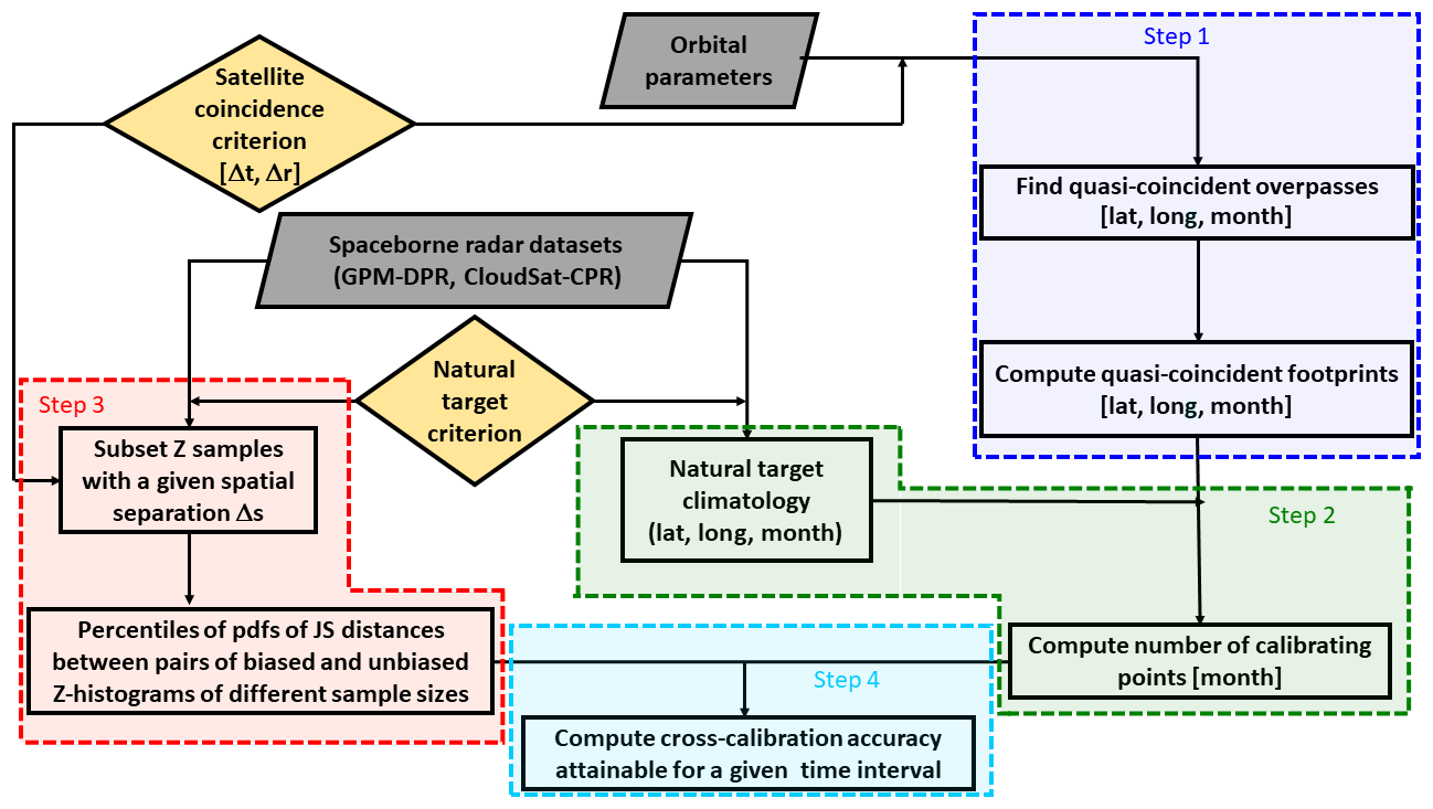
Figure 1 A flow chart showing the methodology followed for the cross-calibration between different spaceborne sensors.

2.1 Orbit quasi-intersections (step 1)

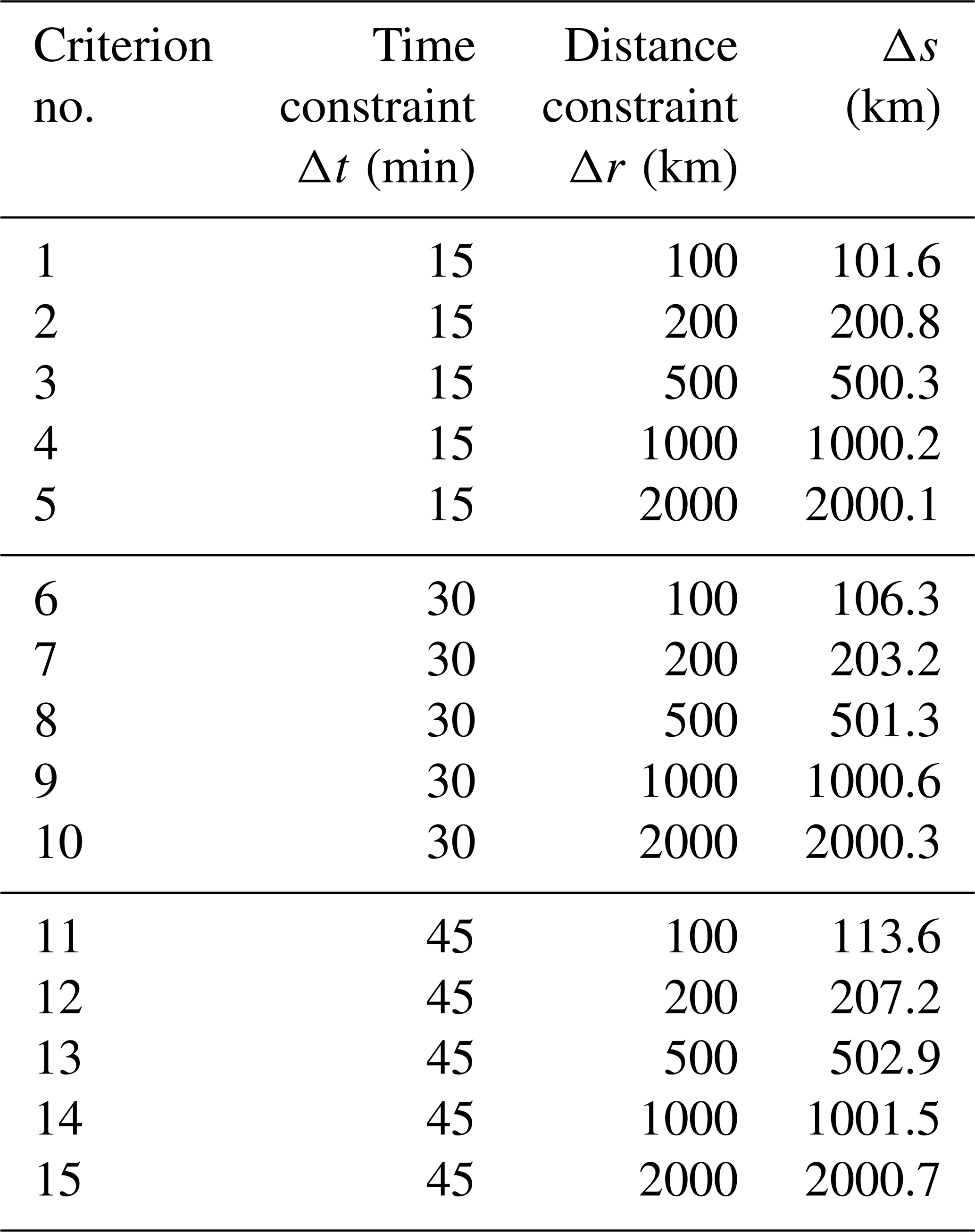
First, we want to establish how many quasi-coincidence footprints can actually be achieved between conically scanning radar systems orbiting in polar or inclined orbits and the reference radars. It is very unlikely that two different radars' sensors on different orbits could illuminate the same target at the same time. Therefore a looser quasi-coincidence criterion is defined by assuming two observations from different platforms to be quasi-coincident if they are taken within a certain time interval, Δt, and a certain distance, Δr, from each other. Different combinations of temporal and spatial constraints adopted in this study are shown in Table 1. Note that here only surface footprint quasi-coincidences are considered. Because of the different observing geometry, quasi-coincidences at different heights could be considered as well. However this effect is considered negligible. In fact, if we consider the maximum altitude of an anvil cloud (circa 20 km), the distance between the radar path intersection at that altitude and a footprint intersection at sea level would be about 20 km, very small if compared to the 1000 and 2000 km distance constraints used in the following analysis.

Table 1 Different combinations of temporal and spatial constraints considered in this study to define a quasi-coincidence. The third column has been computed using Eq. (1) with v_wind=20 m s⁻¹, which is a sensible value for upper-level winds.

The goal of the next investigation is to determine how the quasi-coincidence points vary with different quasi-coincidence criteria. In the following we consider a few different pairs of orbits that can be used for cross-calibration based on existing and planned Ka- and W-band radar systems.

2.1.1 Quasi-coincident overpasses for Ka-band conically scanning radars

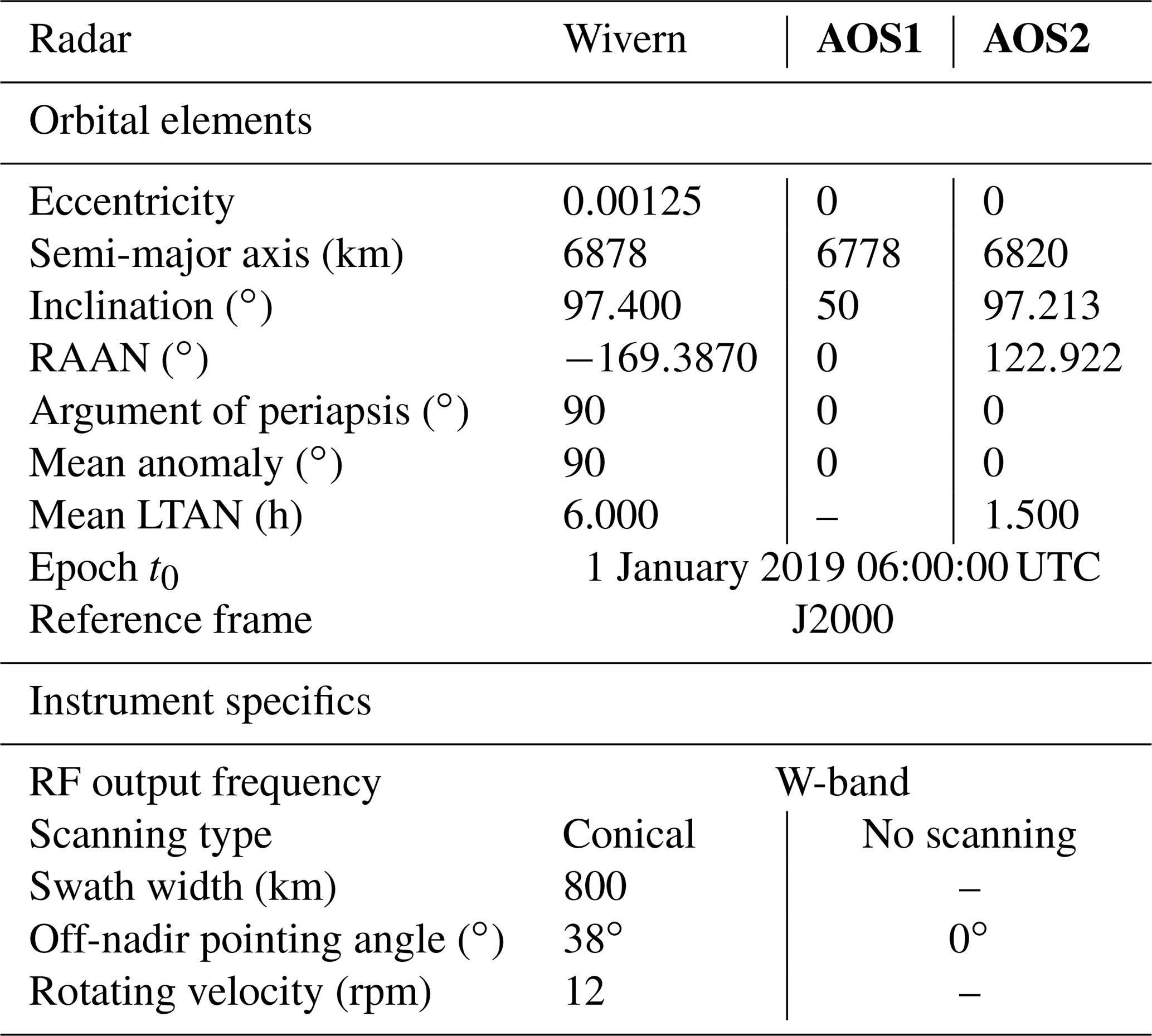
At this band we assume that the GPM Ka-band precipitation radar (KaPR) will be used as the calibrator. The cross-track scanning radar is carried on a 65^∘ inclined orbit at 407 km altitude. Two types of orbits (one polar and one tropical; no specific information is currently available on the orbits of the constellation) are used to demonstrate the methodology for the cross-calibration of the radars of the Tomorrow.io constellation. The first is characterized by an altitude of 500 km and an inclination of 50^∘ and the other by a sun-synchronous orbit and an altitude of 500 km. The two combinations of the Tomorrow.io orbits with the GPM orbit define the first two orbital cross-over configurations. The orbital elements and the instrument specifics are reported in Table 2. The orbits have been propagated analytically using the trajectory equation obtained with the integration of the equation of motion for the restricted two-body problem. Only the J2 perturbations have been taken into account (Bate et al., 1971).

Table 2 Specifics of the Tomorrow.io and GPM satellites orbits and instruments. The radar that is used as a reference because it is properly calibrated is indicated in bold font. The Ka-band GPM radar is expected to be operational at the end of the decade. RAAN: right ascension of the ascending node. LTAN: local time of the ascending node. RF: radio frequency.

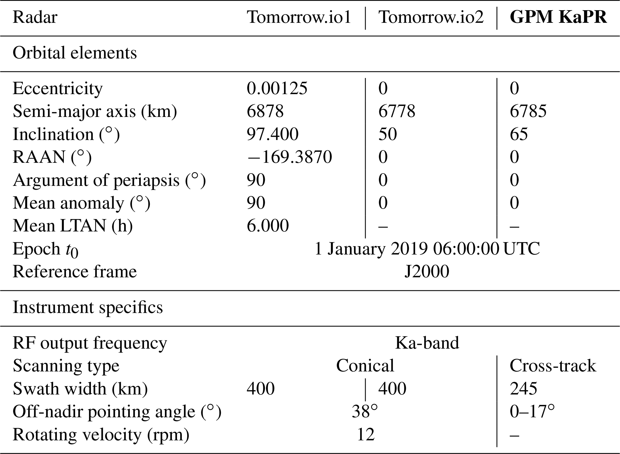
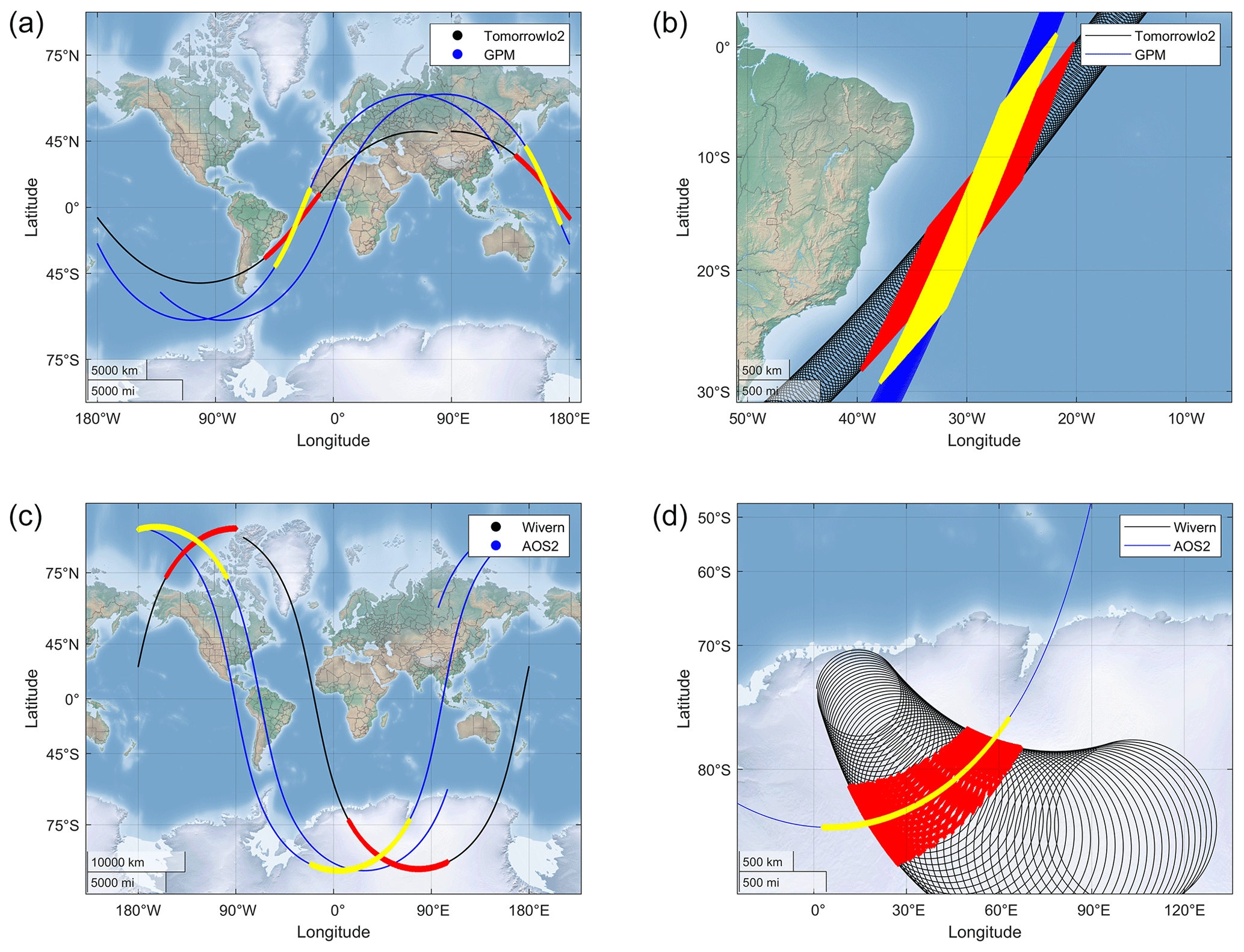
Figure 2 Quasi-intersection footprints between the inclined Tomorrow.io and the Ka-band DPR (a, b) and the AOS2 polar W-band radar and the conically scanning Wivern radar (c, d) according to criterion no. 7. Panels (a) and (c) represent the ground tracks of the two orbits, whereas panels (b) and (d) depict the details of the two radar footprints at the ground in the region where the ground tracks intersect.

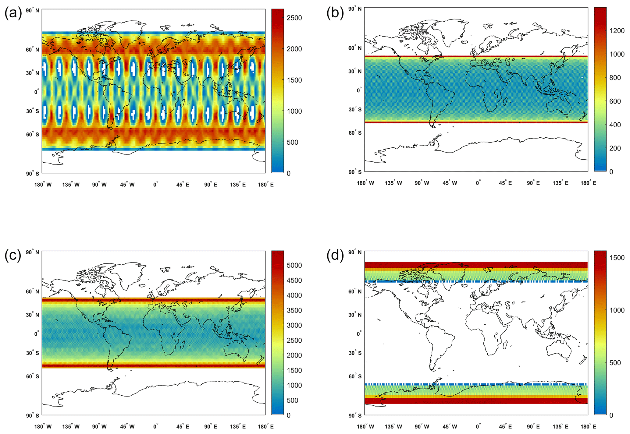
Figure 3 Number of monthly quasi-intersection footprints between Tomorrow.io (polar and inclined) – GPM (a, c) and Wivern – AOS (inclined and polar) (b, d) according to criterion no. 9 (1000 km and 30 min). Each box has a resolution of 2^∘ × 2^∘.

The calculation of the quasi-intersection footprints is split in two steps: first the time intervals where the spacecrafts are close enough are computed (left panels in Fig. 2); then, in correspondence to the segments of orbits found in the first step, the positions of the antenna boresight at the ground are simulated with fine resolution so that the number of quasi-coincident footprints can be computed for any given quasi-coincidence criterion (right panels in Fig. 2). This is demonstrated in the upper panels of Fig. 2 for the quasi-intersection footprints between Tomorrow.io2 and GPM. The numbers of Tomorrow.io monthly quasi-coincidences for the polar and inclined Tomorrow.io and the GPM satellite are shown in the top and bottom left panels of Fig. 3, respectively. They have maxima of occurrences around the extreme latitudes associated with the GPM and the inclined Tomorrow.io orbits, respectively. For the polar-orbiting Tomorrow.io, some strongly longitude-dependent patterns appear due to the specific combination of orbits with the GPM core satellite.

2.1.2 Quasi-coincident overpasses for W-band conically scanning radars

The NASA AOS mission envisages to launch two spacecrafts operating at 400 km altitude with a 50^∘ orbit inclination and at 450 km altitude on a sun-synchronous orbit, respectively. Both spacecrafts will carry a nadir pointing W-band atmospheric radar that can be used as reference calibrator. The Wivern mission plans to fly a satellite in a 500 km altitude and sun-synchronous circular orbit, carrying a conically scanning W-band atmospheric radar (Illingworth et al., 2018). Detailed orbital parameters and instrument specifics are listed in Table 3. The two combinations of the Wivern with the two AOS orbits define the third and the fourth orbital cross-over configurations. An example of orbit quasi-intersection footprints is shown in the bottom panels of Fig. 2, whereas the numbers of Wivern monthly quasi-coincidence footprints between AOS1 and AOS2 and the Wivern satellites are shown in the top and bottom right panels of Fig. 3, respectively. For the polar sun-synchronous AOS2 configuration, quasi-intersection footprints with Wivern are only found between 68 and 82^∘ latitude and peak at the highest latitudes; vice versa, the quasi-intersection footprints between the inclined AOS1 and Wivern are more likely to occur at the highest latitudes touched by AOS1 around 48^∘ latitude.

Table 3 Specifics of the AOS and Wivern satellites orbits and instruments. The radars that are used as a reference are indicated in bold font.

2.2 Calibrating targets (Step 2)

In this section the natural targets that can be used as a reference for cross-calibration are defined. The selection goes to ice clouds away from deep convection because such clouds are characterized by low attenuation both at Ka- and W-band (Protat et al., 2019; Tridon et al., 2020), and therefore their reflectivities do not change with different observation geometries; i.e., the measured reflectivities of an ice cloud observed at nadir and at slant incidence angles are almost identical. Reflectivities are more likely different in the presence of non-spherical particles which are preferentially oriented. However for the calibration we do use reflectivity values that are large, thus corresponding to generally more randomly oriented aggregates. These scatterers tend to have backscattering cross sections independent from incidence angle. With respect to the attenuation, since its value is expected to be small, the Hitschfeld–Bordan attenuation correction (Hitschfeld and Bordan, 1954) could be implemented to account for the differential attenuation signal between the two viewing directions.

Different selection criteria are used at the two bands because of the different sensitivities of the reference radars.

2.2.1 Ka-band conically scanning radars

For Ka-band radars, ice clouds with reflectivity exceeding 15 dBZ (a sensitivity that should be achieved by the Tomorrow.io radars), located at least 500 m above the freezing level and/or the surface and with thicknesses exceeding 1 km, have been used. The Ka-band GPM dual-frequency precipitation radar high-sensitivity products (zFactorMeasured, binZeroDeg, binClutterFreeBottom; https://doi.org/10.5067/GPM/DPR/Ka/2A/07, Iguchi and Meneghini, 2021) have been used to characterize where such clouds are located and how frequently they occur. Only stratiform pixels as identified by the presence of a bright band are considered in our analysis. An example of a midlatitude frontal stratiform system observed by the GPM-Ka radar and of the corresponding ice-calibrating clouds is depicted in the left panel of Fig. 4. The climatology of the mean number of the 500 m thick radar bins of ice-calibrating clouds is presented in the top panel of Fig. 5. These statistics are based on more than 4 years of GPM-Ka-band data, from the satellite launch in 2014 to the 21 May 2018 when the scanning strategy was modified (see Liao and Meneghini, 2022) The figure shows patterns with maxima and minima in line with the climatology of ice water path derived from CloudSat and CALIPSO reported in Hong and Liu (2015, Fig. 3). Thick ice clouds are frequently observed in regions of deep convection (e.g., the Inter Tropical Convergence Zone) and along storm tracks in the midlatitudes. Note that in some locations in the tropics, where thick ice clouds are ubiquitous, the mean number of 500 m thick ice-calibrating clouds is higher than one. This means that a quasi-intersection footprint occurring in such areas will produce on average more than one calibrating point.

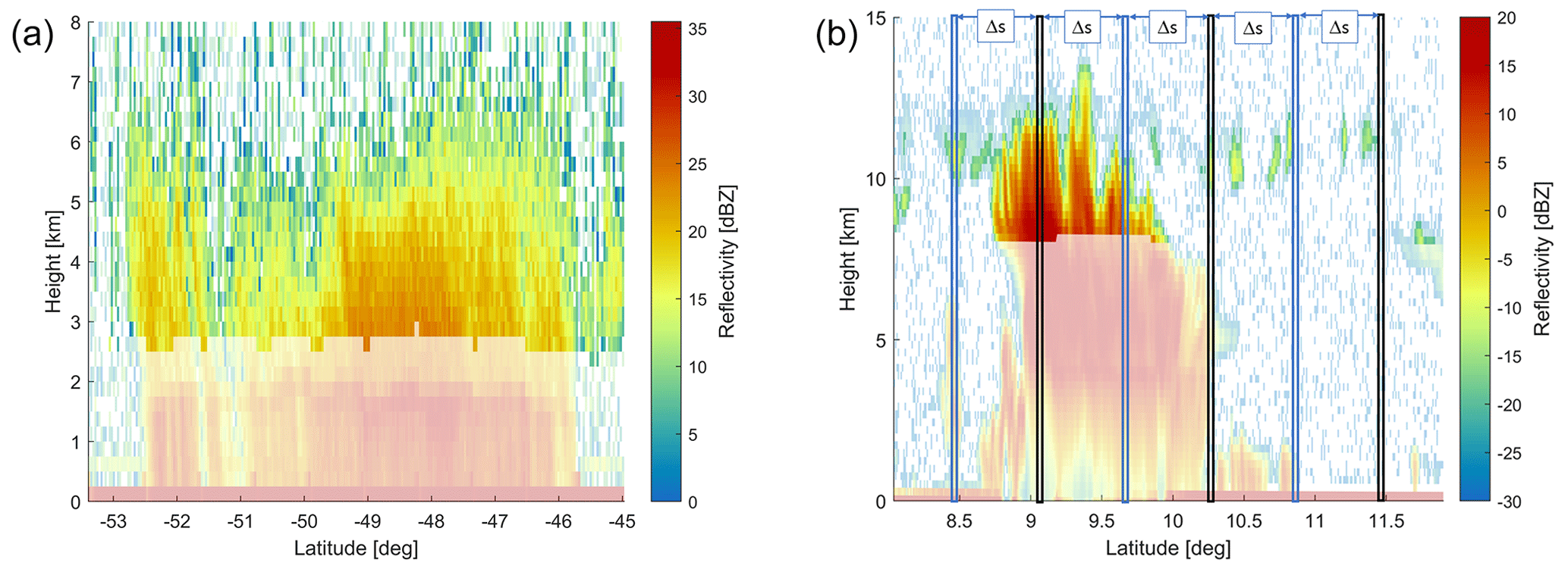
Figure 4 Example of GPM Ka-band (a) and CloudSat W-band (b) reflectivity profiles over a midlatitude and a tropical system, respectively. The regions with bright colors represent the points that are used as natural target calibrating points. In panel (b) the procedure adopted in step 3 is illustrated (see description in Sect. 2.3 for details). Each dashed box represents a 5 km along track slice. The reflectivities of the calibrating points are clustered together in correspondence to the black and blue boxes, which are separated by a given distance Δs (for this specific example of the order of 500 km).

Figure 5 Global distribution of the mean number of 500 m thick radar range bins per profile of Ka-band (a) and W-band (b) ice-calibrating clouds as derived by 4 years of GPM and CloudSat data, respectively. The resolution is 2^∘ × 2^∘. For a given 2^∘ × 2^∘, if the mean number of 500 m thick ice cloud bins per profile is equal to one, for any vertical profile collected in that region, an average of one 500 m thick calibrating ice cloud bin will be detected.

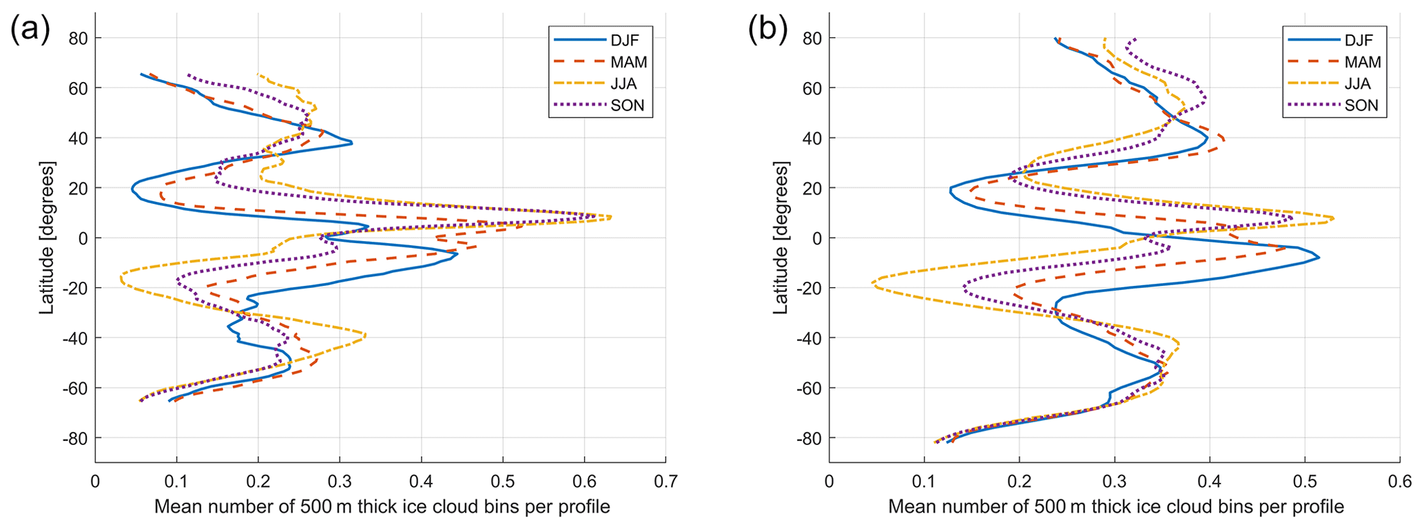
Figure 6 Zonal variability of the mean number of 500 m thick radar range bins per profile for Ka-band and W-band ice-calibrating clouds, respectively. Four different seasons are plotted, as indicated in the legend. The same datasets adopted to produce Fig. 5 have been used.

Zonal plots of seasonal variation of the mean number of 500 m thick ice-calibrating clouds are plotted in the left panel of Fig. 6 for the four seasons DJF (December–January–February), MAM (March–April–May), JJA (June–July–August) and SON (September–October–November). In the tropics it is clear that the maximum moves with the intertropical convergence zone from south, during DJF, to the north of the Equator in JJA. These numbers represent multiplicative zonal factors that needs to be applied to the number of satellite quasi-intersection footprints to find the number of calibrating points.

Table 4 Number of weekly calibrating points. For each configuration, the number of calibrating points for each of the radars involved in the cross-calibration is reported in the two corresponding columns. A calibration point correspond to a 5 and 1 km along-footprint track for the Ka- and W-band, respectively.

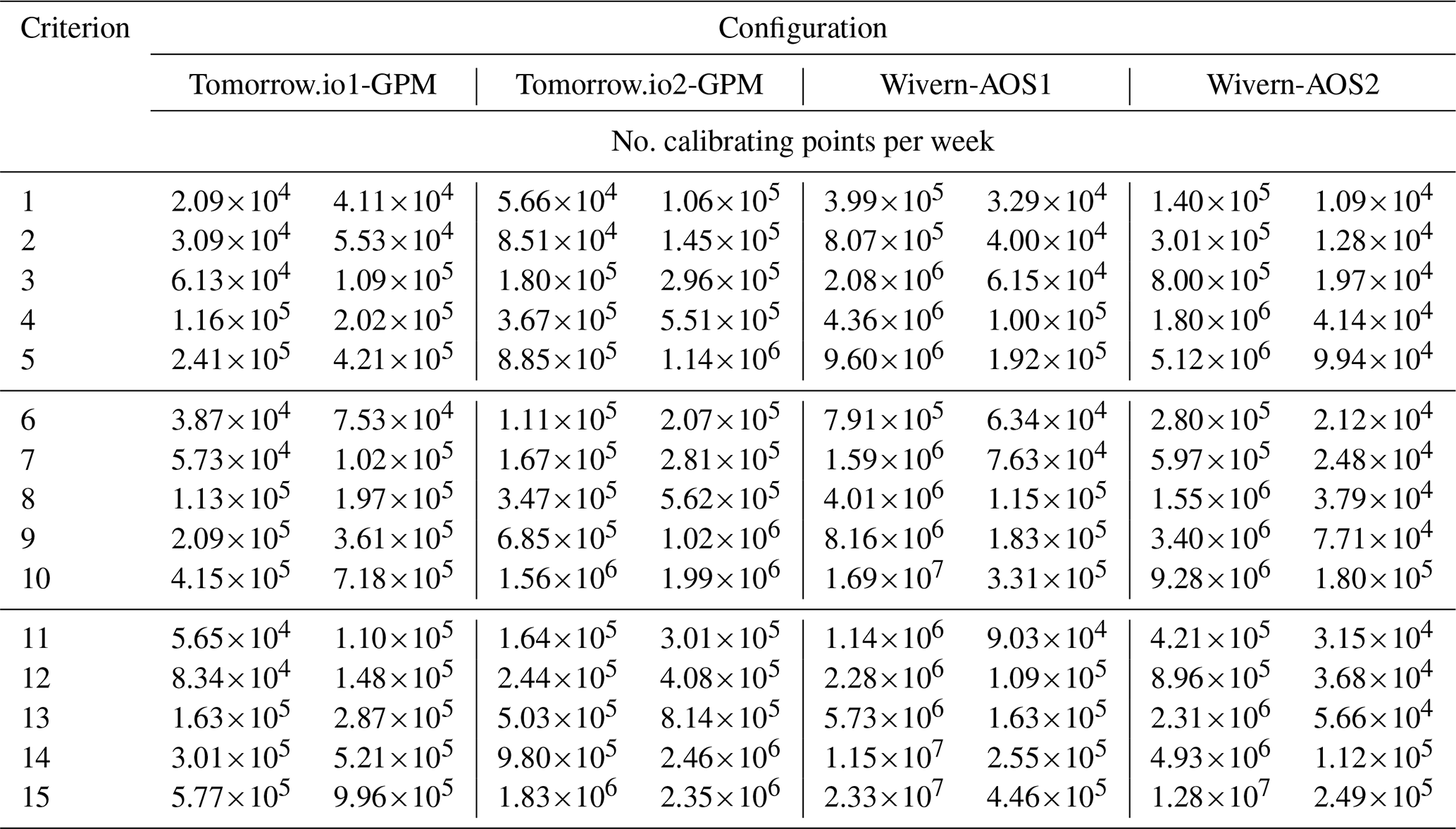
The total number of weekly calibration points (obtained by multiplying the weekly number of quasi-intersection footprints and the climatological number of 500 m thick ice-calibrating clouds) involving the two Tomorrow.io radars is reported in the four columns (from the second to the fifth) in Table 4. Note how the number of calibrating points for GPM and for Tomorrow.io is similar (due to the similar sampling rate) and, as expected, is constantly increasing with Δt and Δr.

2.2.2 W-band conically scanning radars

For W-band radars, we have used ice clouds with reflectivity exceeding −20 dBZ (Wivern radar will certainly achieve such a sensitivity; Illingworth et al., 2018) located in regions with temperature colder than 250 K, with a vertical extension of at least 750 m and located more than 2 km above clutter. The CloudSat CPR (with a much better sensitivity of around −30 dBZ) dataset can be exploited to understand where such clouds are located and how frequently they occur. Different CloudSat products (see https://www.cloudsat.cira.colostate.edu/, last access: 1 February 2022, CloudSat Data Processing Center, 2022) are used to derive geo-located reflectivity profiles and to identify the surface clutter height (2B-GEOPROF), to determine the temperature profile (ECMWF-AUX) and to filter out deep convective cores by excluding deep convective clouds as identified in the cloud type variable of the 2B-CLDCLASS product. An example of a tropical system observed by CloudSat and of the corresponding ice-calibrating clouds is depicted in Fig. 4b.

A total of 4 years of data from 2007 to 2010 have been analyzed to compute the climatology of such clouds as observed by the CloudSat radar. The global distribution of the mean number of 500 m thick ice W-band calibrating clouds is shown in Fig. 5. As expected, the patterns are very similar to those shown for Ka-band calibrating clouds. Also the mean number of ice bins is not very dissimilar because the better sensitivity at W-band is offset by the tighter constraint on the temperature. The zonal plots of the seasonal variation of the mean number of 500 m thick ice-calibrating cloud bins (right panel of Fig. 6) are similar to the results found at Ka-band as well. An alike seasonal movement with the intertropical convergence zone is also observed. Thicker ice clouds occur in northern and high latitudes during the warm season (JJA) and the autumn (SON), with thinner clouds observed more frequently during the cold season (DJF) and the spring (MAM). In contrast, southern midlatitudes and high latitudes have less variable ice cloud frequencies over the whole year.

The total numbers of calibration points involving the Wivern radar are reported in the four columns from the sixth to the ninth in Table 4. Thanks to its much higher footprint ground velocity (≈ 800 km s⁻¹) and its faster sampling rate, Wivern calibrating points are significantly more than those obtained for the AOS radars (with increasingly larger differences for larger Δr).

2.3 JS distances for biased and unbiased reflectivity PDFs (step 3)

The GPM and CloudSat datasets have been further exploited to determine what the difference between the reflectivity PDFs is when sampling calibrating clouds separated by a given distance. In the cross-calibration procedure, the targets observed by the two radars will not be identical because they will correspond to quasi-coincident footprints; i.e., they will be sampled in locations separated by a certain distance Δs (see Eq. 1). The aim of this section is to study the similarity of cloud reflectivity PDFs for targets sampled at a certain distance from each other by building synthetic correlated pair of PDFs which should simulate the PDFs as collected by the calibrating and by the to-be-calibrated radar in the cross-calibration procedure. For each of the quasi-coincidence criteria we have constructed these PDFs using points collected by CloudSat or GPM that are separated by a distance Δs like illustrated in the right panel of Fig. 4. In each of the 5 km wide vertical slices, only a limited number of calibrating points are present. In order to smooth the PDFs and reduce their sampling noise, a large number of calibrating points are needed. This is achieved by putting together reflectivity values corresponding to 5 km thick slices separated by Δs (like the slices delimited by the blue and the black lines in the right panel of Fig. 4) and belonging to different orbits. By doing this, two PDFs, f₁(Z) and g₁(Z), are obtained with a characteristic number of sampling points (higher number of points obviously requiring larger number of orbits). This number of sampling points (which will correspond to a given acquisition calibration period) is increased to assess the impact that the number of calibrating points has in reducing the sampling noise. The exercise is then repeated multiple times (thus involving different orbits or by reshuffling the starting points of the “Δs” sequence within a given orbit) to find an ensemble of such PDF pairs. Let name these realizations f_i(Z) and g_i(Z) with i=1, 2, …, N. For each pair, the Jensen–Shannon distance d_JS[i] is computed (see Eq. 2). If N is large enough, the PDF of all d_JS gives an idea about the expected distance between 2 PDFs (the mean of the PDF) and its natural variability (the width of the PDF), thus mimicking the fact that in our calibration methodology, clouds not from coincident but from quasi-coincident overpasses are sampled.

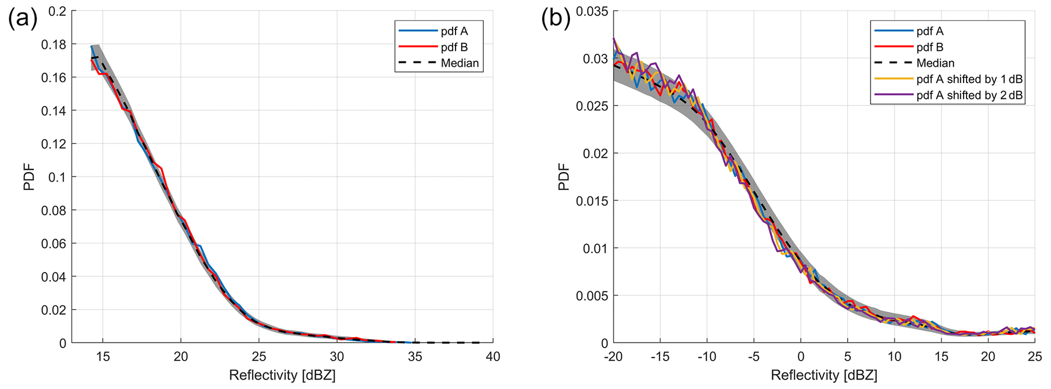
Figure 7 Envelope (5–95th percentile) of Z PDFs for the Ka-band ice-calibrating clouds (a) and for the W-band ice-calibrating clouds (b) for two sets of cloud reflectivities sampled with a separation of 500 km. The black line represents the median Z PDF, whereas the blue and red curve represent two PDFs randomly selected. Both PDFs have been built with about 50 000 calibration points (Table 4 can be used to compute the time needed to collect such sample according to the different configurations and quasi-coincidence criteria). For the W-band PDF the effect of a positive bias of 1 and 2 dB is also shown.

Examples of a pair of Z PDFs are shown in Fig. 7 for both Ka- and W-band reflectivities when including 50 000 calibration points (red and blue lines). The median global climatology PDF is plotted as a dashed black line, whereas the 5th and 95th percentile of the PDF are shown by the grey shading. Note how the Z PDF monotonically decreases both at Ka- and W-band with increasing reflectivity values. While the spread between the high and low percentiles decreases with increasing Z, the relative noisiness of the PDFs increases when going towards Z values with low probability of occurrence. These values will not contribute much in the JS distances because of the multiplicative factor P(x) in Eq. (3). For the W-band PDF the effect of a positive bias of 1 and 2 dB is also illustrated by the yellow and the purple curve, respectively. The two curves depart significantly from the median behavior, and they dwell outside the shaded regions for a significantly greater number of points when increasing the bias from 1 to 2 dB. For instance, for the example shown in the right panel, the JS distance between the median PDF (dashed black line) and the blue, red, yellow and purple curves is equal to 0.0338, 0.0334, 0.0476 and 0.0646, respectively.

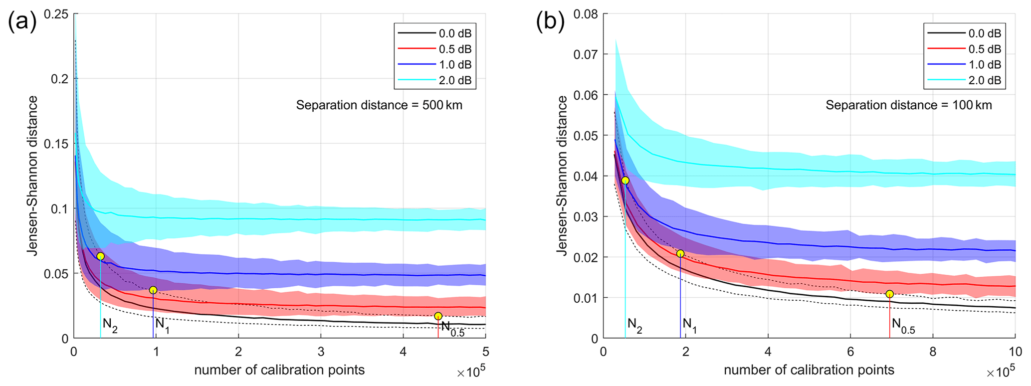
Figure 8 Characterization of the JS distance for Ka- (a) and W-band (b) Z PDF pairs for ice-calibrating targets separated by Δs=500 km and Δs=100 km, respectively, as a function of the number of calibrating points of each PDF. The median distance is indicated by the black line, whereas the dashed black lines indicate the 5th and 95th percentiles. The colored lines with the shaded envelopes correspond to the median and the same percentiles when shifting one of the two Z PDF by different reflectivity biases as indicated in the legend. Here positive biases are shown, but similar results are obtained when negative biases are applied.

In order to understand what the expected JS distances are when comparing pairs of Z PDFs collected by two radars from clouds at given separation distances, the previously described procedure is repeated for different sample sizes and for an ensemble of pairs large enough to characterize the distribution function of the JS distances for any given sample size and separation, Δs. The median value (black line) of the JS distance for the ensemble of pairs of Ka- and W-band Z PDFs is shown in Fig. 8 as a function of the number of calibrating points for a separation distance of 500 and 100 km, respectively. The dashed black lines indicate the 5th and 95th percentiles of the ensemble and define the range of the intrinsic natural variability and noisiness associated with the sampling process. As expected, the median values of the JS distances (continuous black line) decrease with increasing number of calibrating points (i.e., the PDFs become less and less noisy; thus the JS distance decreases). The envelop between the dashed lines represents the range of values of the JS distances well between Z PDF pairs for ice-calibrating clouds separated by 500 km at Ka-band (left) and by 100  km at W-band (right) for different numbers of calibrating points.

The same exercise is repeated by shifting one of the two reflectivity Z PDFs of the pair by a calibration reflectivity bias (e.g., 0, ±0.5 ±1 dB, …) to assess what the impact of a miscalibration onto the JS distances is. All JS distances jump up with a shift that increases with the bias magnitude, as demonstrated in Fig. 8 where positive biases of +0.5, +1 and +2 dB are considered. Similar results are obtained when negative biases are applied. From the plot it is clear that, for each value of the reflectivity bias, there is a threshold of calibration points above which the range of values in the corresponding colored envelope is clearly distinct from the unbiased range delimited by the dashed black lines. For the three biases shown in the right panel of Fig. 8 these values are indicated by the numbers N_0.5, N₁ and N₂ with $N_{\mathrm{0.5}}>N_{\mathrm{1}}>N_{\mathrm{2}}$. For instance, with 100 000 calibration points defined by a separation distance of less than 100 km, a bias of 2 dB produces JS distances above 0.038 (5th percentile value), which are incompatible with the range of values expected from the natural variability between 0.019 and 0.028 (respectively the 5th and 95th percentiles found in correspondence to the dashed black lines). On the other hand a 1 dB bias is expected to produce JS distances between 0.024 and 0.037 and therefore cannot be unequivocally identified. Collecting a sample larger than N₁ = 187 210 would guarantee being able to identify a bias of 1 dB. A much larger value (N_0.5 = 667 700) would be required to discern a miscalibration of 0.5 dB. Also, the red envelope remains very close to the envelope identified by the dashed black lines with increasing numbers of calibrating points, which makes the calibration method more difficult to be applied at such high accuracy levels.

Therefore the plots in Fig. 8 can be used to understand what reflectivity biases are discernible when collecting a certain number of reflectivities corresponding to calibration points located within a given distance. Generally speaking, the calibration for the Ka-band radars performs better than the one for W-band radar (i.e., a smaller number of calibrating points is needed to achieve a given calibration accuracy). This is due to the sharper sloping of the Z PDF of the Ka-band calibrating targets compared to that of the Z PDF of the W-band calibrating targets (a factor of 10 decrease in the 10 dB (30 dB) reflectivity range for Ka-band (W-band)). With our method, a constant Z PDF would be useless, whereas a square wave-shape Z PDF would perform optimally.

Results for the JS distances as a function of the number of calibrating points when changing Δs are shown in Fig. 9. For the same number of calibrating points, smaller Δs values are characterized by a smaller JS distance, as expected by an increased correlation of the reflectivities, aggregated at shorter separation distances, between the two sampled Z PDFs. Note that the variability between the median curves (continuous lines) corresponding to different separation distances tends to be of the same magnitude as the variability between the 5th and 95th percentiles of each single PDF (dashed envelopes), with the distances between the median curves becoming smaller and smaller at large separation distances. This feature suggests that, in a calibration procedure, it is more effective to use large values of Δs because this choice will enable us to collect the same number of calibrating points in a quicker time.

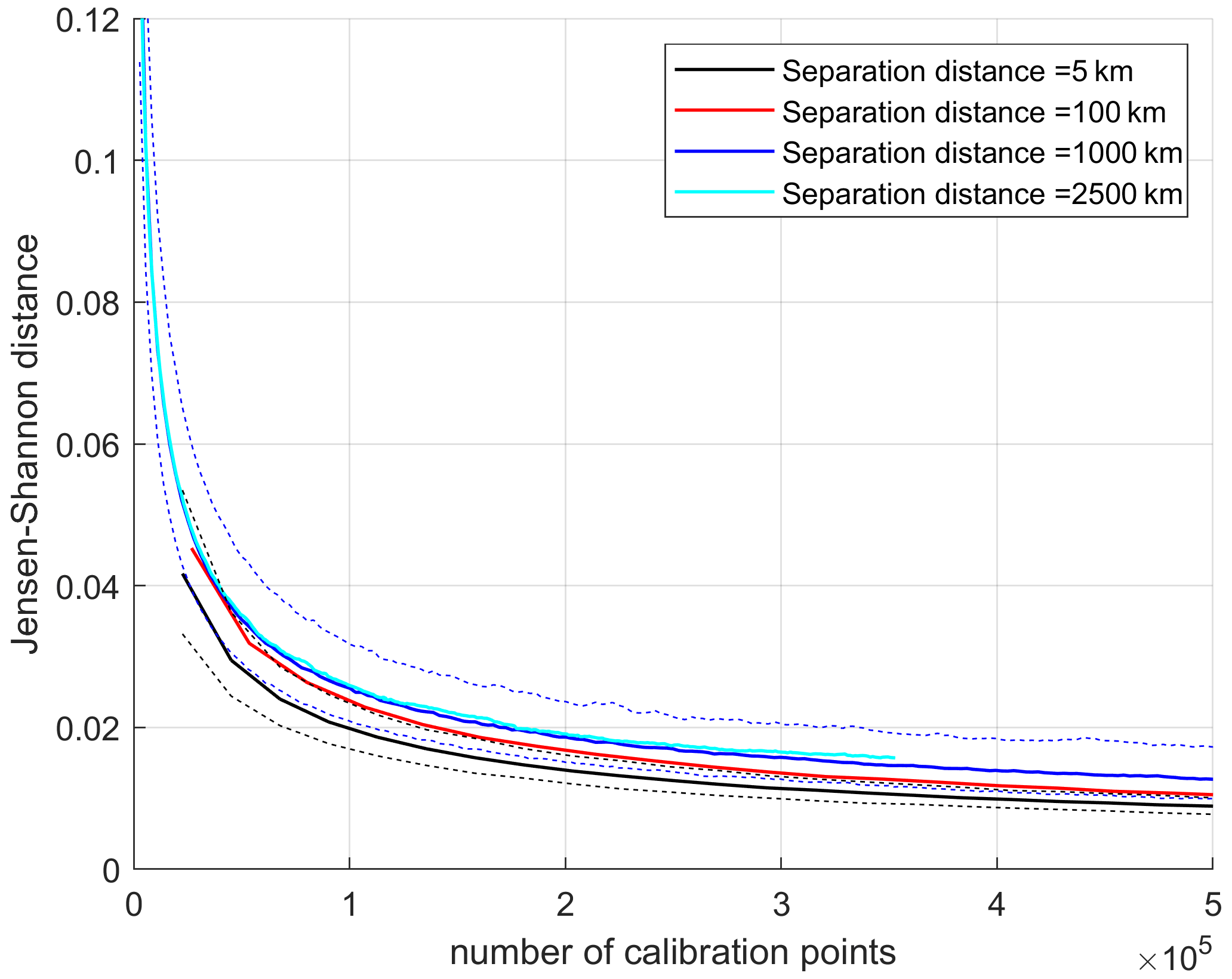
Figure 9 Impact of the separation distance of points in the pairs of Z PDFs on the JS distances as a function of the number of points for the PDFs of W-band calibrating targets. The four continuous colored lines correspond to the median of the JS distances for different separation distances, as indicated in the legend. The black and the blue dashed lines correspond to the 5th and 95th percentiles for the 5 and the 1000 km separation distances.

3 Results of cross-calibration performance

The results of step 3 and step 4 can be combined to assess what accuracy can be achieved in the cross-calibration in a given time period and which is the optimal quasi-coincidence criterion to be used among those listed in Table 1. For each criterion and for each reflectivity bias the number of calibration points above which the envelopes of the unbiased and biased JS distances become distinct is computed. These numbers are converted to the number of days required to collect such calibration points based on the figures tabulated in Table 4. In a conservative approach, for each radar-pair configuration, the lowest number of the two columns presented in the table is used. This is particularly penalizing for the Wivern system, but it is a consequence of the fact that the noisiness of the JS distances will be driven by the reduced sampling capability of the AOS radars.

Table 5 Mean number of days required to achieve a given calibration accuracy for the different criteria listed in Table 1 and for the four configurations analyzed in this study. A “–” symbol means that the given level of accuracy in the calibration cannot be achieved. Results with positive and negative miscalibration are very similar. Here for concision only positive miscalibrations are considered.

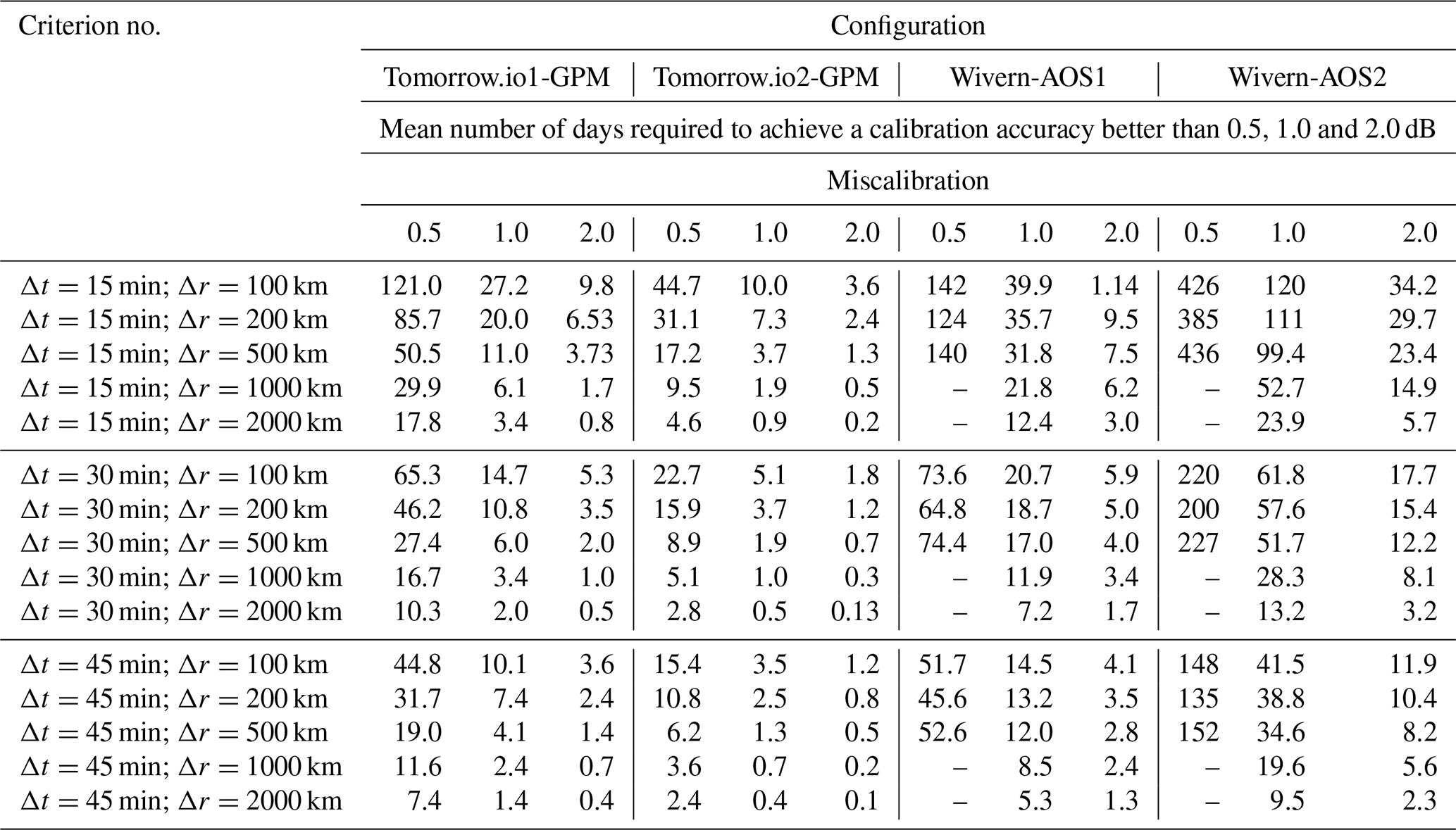
Results (reported in Table 5) show that criteria based on large Δs are generally preferable; i.e., the increased number of quasi-coincidences when adopting criteria with large Δs tends to overcome the reduced correlation of cloud Z PDFs. Thanks to the large swath of GPM and Tomorrow.io radars, for Tomorrow.io radars, cross-calibrations with GPM Ka-band radar within 1 dB are realistically achieved on average within few days (less than 2 when considering criterion no. 10 and no. 15), a very promising result for the Tomorrow.io constellation. Even a cross-calibration within 0.5 dB seems feasible within a week for the polar Tomorrow.io and a few days for the inclined Tomorrow.io. In general, cross-calibration with GPM can be performed on shorter timescales for the inclined Tomorrow.io configuration.

For Wivern, cross-calibrations with an accuracy better than 1 dB is feasible on timescales of the order of less than 7 d for AOS1 and of less than 10 d for AOS2 (both achieved with criterion no. 15). A calibration within 2 dB on the other hand can be achieved much more quickly (within two and 3 d for AOS1 and AOS2, respectively).

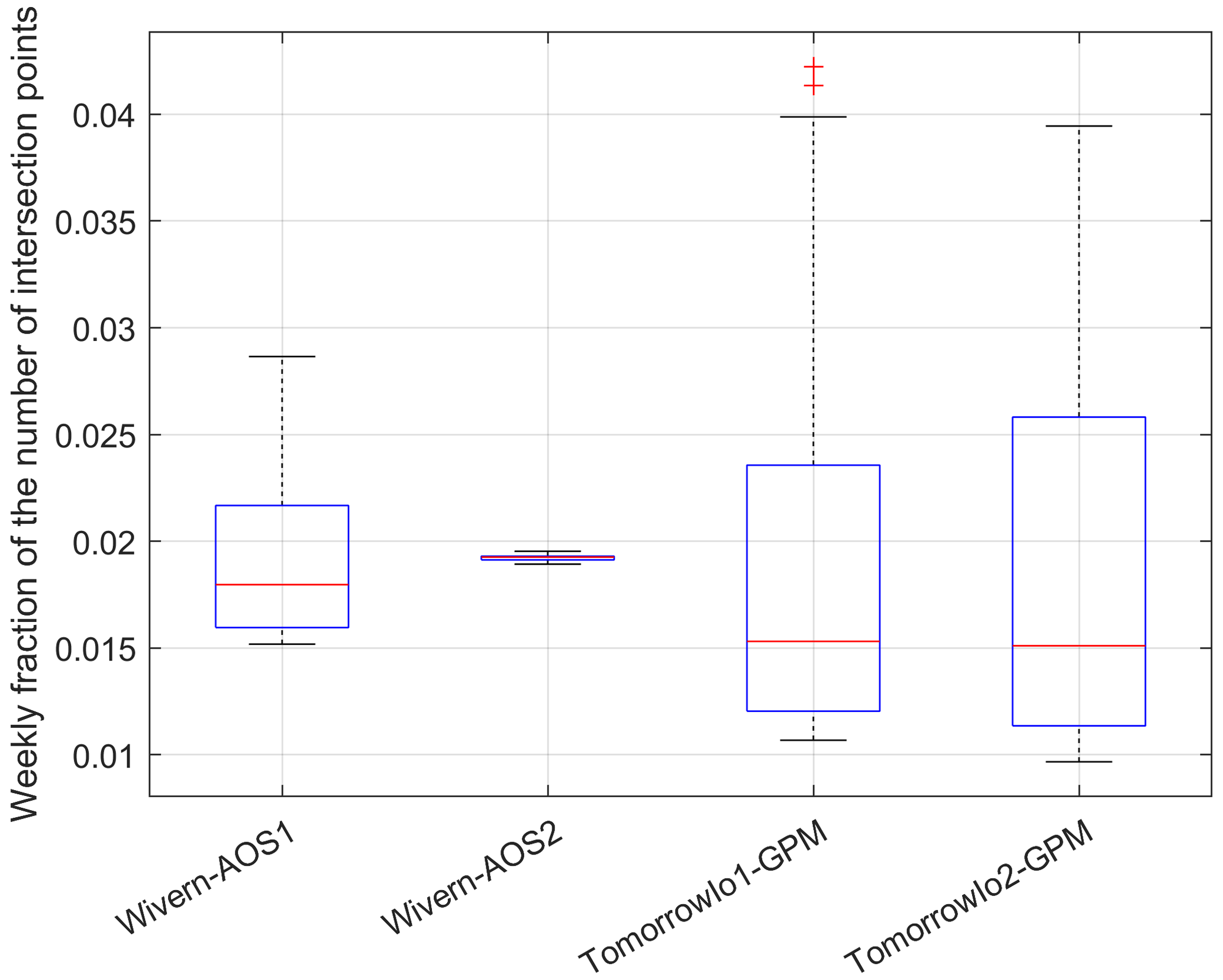
Figure 10 Whisker plot with the weekly fraction of the year calibration points for the 52 weeks of the year for the four satellite configurations considered in this study and for criterion no. 15. The mean value for all distribution is 0.019 (i.e., $\mathrm{100}/\mathrm{52}$). The annual number of calibration points is about 75, 63, 602 and 743 million for AOS1, AOS2, Tomorrow.io1 and Tomorrow.io2, respectively.

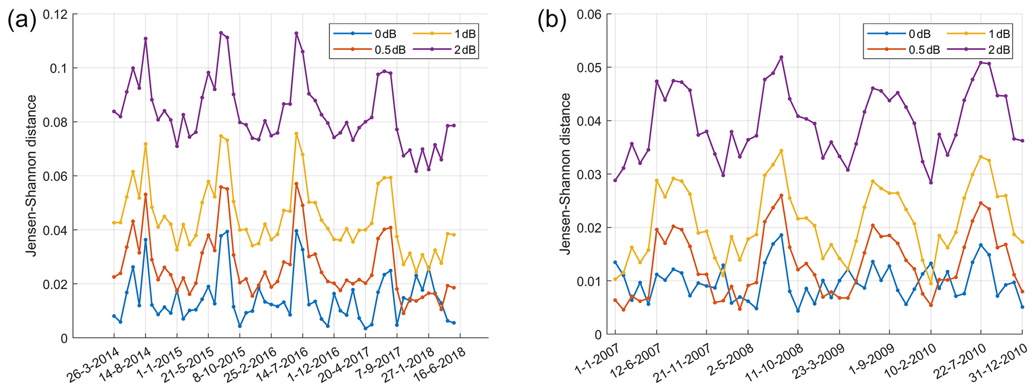
Figure 11 Time evolution of the JS distances of monthly cumulated Z PDFs to 4 years of Ka- (a) and W-band (b) climatology.

It is important to note that these are mean results based on annual climatology of clouds and of orbital quasi-intersection footprints; in specific conditions, with a lack of orbital quasi-intersections and the absence of ice clouds, the time needed for achieving these results can be longer. However, for criterion no. 15 that achieves the best results, there is small variability on a weekly basis, as demonstrated by the whisker plot in Fig. 10. The combination between the polar Tomorrow.io and GPM shows large variability from week to week with a cycle that exceeds 1 year. The largest variability is encountered with the inclined Tomorrow.io orbit. In the worst-case scenario, for such a configuration, some weeks produce less than 1 % of the annual number of calibration points.

Since the best results are obtained with the largest temporal and spatial separation distance, it is sensible to ask whether the curves of the global climatology of ice clouds Z PDFs could be used as absolute calibration curves, without the need of satellites' cross-over. In order to investigate this possibility, the following steps are followed:

• A climatological Z PDF (PDF₁) covering 4 years of data is produced.

• For each day in the dataset, a separate Z PDF is generated (PSD_j), and JS distances between PDF₁ and PDF_j are computed at different aggregation intervals (weekly and monthly).

• PDF_j is shifted by ±0.5, ±1 and ±2 dB, and the corresponding JS distances between PDF₁ and the six shifted PDFs are computed.

• Time series of the seven different JS distances are produced and compared.

Results accumulated at the monthly scale depicted in Fig. 11 for the Ka-band (left) and W-band (right panel) show that a climatological calibration seems feasible within 1 dB at such temporal scale (2 dB is attainable at the weekly scale, not shown). The presence of an annual cycle is also evident both at Ka-band and at W-band. For the GPM Ka-band radar, an anomalous behavior appears after July 2017 with the 0.5 dB curve, intersecting and becoming smaller in magnitude than the 0 dB curve. This climatological approach could therefore represent a way to monitor long-term calibration issues for a single radar system as well.

4 Summary and conclusions

This study presents a methodology for calibrating a spaceborne conically scanning radar using cross-calibration with reference spaceborne radars working on the same band and orbiting around Earth at the same time. Example of such systems are the Ka-band GPM radar or the W-band radars planned for the ESA-JAXA EarthCARE or for the NASA AOS missions. Ice clouds at cold temperatures (not prone to appreciable attenuation) are used as natural targets that allow the systems to be cross-calibrated.

Radar antenna boresight positions have been propagated based on satellite orbits; then, the ground-track quasi-intersections have been calculated for different quasi-intersection criteria, as defined by cross-overs within a certain time and a given distance. Then the climatology of the calibrating clouds has been studied using the W-band CloudSat and Ka-band GPM reflectivity dataset in order to derive the global distribution of the frequency of the ice-calibrating clouds (climatology presented in Fig. 5). The number and the spatial distribution of calibration points are finally obtained by multiplying the ground-track quasi-intersection footprints and the climatology of clouds.

The similarity between the reflectivity distribution functions of the calibrating ice clouds at different separation distances has been studied using the CloudSat and GPM dataset in order to find the optimal distance criterion which optimizes the calibration accuracy and minimizes the time needed to achieve such an accuracy. This requires a trade-off between having a sufficiently large number of observations to reach statistical significance (obtained by relaxing the quasi-coincidence criterion) and a reasonable invariance of the cloud reflectivity statistical properties (achieved by tightening the quasi-coincidence criterion).

Findings of this work demonstrate that it will be possible to cross-calibrate a Ka-band (W-band) conically scanning radar within 1 dB like that envisaged for the Tomorrow.io constellation (Wivern mission) every few days (a week). Such uncertainties generally meet the mission requirements and the standards currently achieved with absolute calibration accuracy. The better performances achieved for the Tomorrow.io is the result of the higher number of quasi-intersection footprints (thanks to the combined scanning pattern of the Tomorrow.io radars and GPM and to the shape of the Z PDF better suited to perform cross-calibration).

In principle, the global climatology Z PDF (continuous black lines in Fig. 7) could be used as an absolute reference, and the JS distance could be computed with respect to such a PDF. This would completely remove the issue of having quasi-intersections, but it is not certain how the natural variability introduced by regional, diurnal and seasonal cycles could impact the uncertainties of the Z PDF itself. More research needs to be done in this area, mainly hampered by the lack of global observations of the ice cloud diurnal cycle.

Calibration of radar reflectivities is paramount for producing unbiased hydrometeor mass contents and mass fluxes, which represent flagships products in most cloud and precipitation radar missions. The approach described in this work is applicable to estimate the cross-calibration accuracy for any orbital cross-over and will be applicable already for the calibration of the Ka-band Tomorrow.io and the INCUS train (Stephens et al., 2020) radars, expected to be launched starting from the end of 2023 and in 2027, respectively.