Characterising the methane gas and environmental response of the Figaro Taguchi Gas Sensor (TGS) 2611-E00

In efforts to improve methane source characterisation, networks of cheap high-frequency in situ sensors are required, with parts-per-million-level methane mole fraction ([CH₄]) precision. Low-cost semiconductor-based metal oxide sensors, such as the Figaro Taguchi Gas Sensor (TGS) 2611-E00, may satisfy this requirement. The resistance of these sensors decreases in response to the exposure of reducing gases, such as methane. In this study, we set out to characterise the Figaro TGS 2611-E00 in an effort to eventually yield [CH₄] when deployed in the field. We found that different gas sources containing the same ambient 2 ppm [CH₄] level yielded different resistance responses. For example, synthetically generated air containing 2 ppm [CH₄] produced a lower sensor resistance than 2 ppm [CH₄] found in natural ambient air due to possible interference from supplementary reducing gas species in ambient air, though the specific cause of this phenomenon is not clear. TGS 2611-E00 carbon monoxide response is small and incapable of causing this effect. For this reason, ambient laboratory air was selected as a testing gas standard to naturally incorporate such background effects into a reference resistance. Figaro TGS 2611-E00 resistance is sensitive to temperature and water vapour mole fraction ([H₂O]). Therefore, a reference resistance using this ambient air gas standard was characterised for five sensors (each inside its own field logging enclosure) using a large environmental chamber, where logger enclosure temperature ranged between 8 and 38 ^∘C and [H₂O] ranged between 0.4 % and 1.9 %. [H₂O] dominated resistance variability in the standard gas. A linear [H₂O] and temperature model fit was derived, resulting in a root mean squared error (RMSE) between measured and modelled resistance in standard gas of between ±0.4 and ±1.0 kΩ for the five sensors, corresponding to a fractional resistance uncertainty of less than ±3 % at 25 ^∘C and 1 % [H₂O]. The TGS 2611-E00 loggers were deployed at a landfill site for 242 d before and 96 d after sensor testing. Yet the standard (i.e. ambient air) reference resistance model fit based on temperature and [H₂O] could not replicate resistance measurements made in the field, where [CH₄] was mostly expected to be close to the ambient background, with minor enhancements. This field disparity may have been due to variability in sensor cooling dynamics, a difference in ambient air composition during environmental chamber testing compared to the field or variability in natural sensor response, either spontaneously or environmentally driven. Despite difficulties in replicating a standard reference resistance in the field, we devised an excellent methane characterisation model up to 1000 ppm [CH₄] by using the ratio between measured resistance with [CH₄] enhancement and its corresponding reference resistance in standard gas. A bespoke power-type fit between resistance ratio and [CH₄] resulted in an RMSE between the modelled and measured resistance ratio of no more than ±1 % Ω Ω⁻¹ for the five sensors. This fit and its corresponding fit parameters were then inverted and the original resistance ratio values were used to derive [CH₄], yielding an inverted model [CH₄] RMSE of less than ±1 ppm, where [CH₄] was limited to 28 ppm. Our methane response model allows other reducing gases to be included if necessary by characterising additional model coefficients. Our model shows that a 1 ppm [CH₄] enhancement above the ambient background results in a resistance drop of between 1.4 % and 2.0 % for the five tested sensors. With future improvements in deriving a standard reference resistance, the TGS 2611-E00 offers great potential in measuring [CH₄] with parts-per-million-level precision.

1 Introduction

Methane (CH₄) is a potent greenhouse gas (Mitchell, 1989) with many poorly characterised sources (Jackson et al., 2020). Yet as global background levels of atmospheric methane mole fraction ([CH₄]) are increasing (Rigby et al., 2007; Nisbet et al., 2014), improved source flux quantification is required (Saunois et al., 2016; Nisbet et al., 2019; Turner et al., 2019). This necessitates improvements in fast-response (less than 1 min) and high-frequency (at least 0.1 Hz) in situ [CH₄] sampling. CH₄ is a trace gas with a low natural ambient atmospheric background (defined to be 2 ± 1 ppm from here on), which is 2 orders of magnitude lower than global background levels of carbon dioxide mole fraction ([CO₂]) (Dlugokencky et al., 1994; Lan et al., 2023).

Fast-response in situ [CH₄] sampling techniques span many capabilities and costs (Hodgkinson and Tatam, 2013; Schuyler and Guzman, 2017). The best measurements are achieved using tuneable infrared (IR) lasers (Baer et al., 2002; Frish, 2014), but cheaper broadband IR can also be used in techniques such as non-dispersive IR spectroscopy (Hummelgård et al., 2015) at the expense of precision (Shah et al., 2019). Alternatively, semiconductor-based metal oxide (SMO) sensors have been available for several decades (Fleischer and Meixner, 1995; Barsan et al., 2007; Reinelt et al., 2017; Ponzoni et al., 2017). Though they are marketed for low-precision applications, their low cost of less than EUR 100 (Eugster and Kling, 2012; Riddick et al., 2020) merits a thorough assessment of their fast-response [CH₄] sampling capability (Collier-Oxandale et al., 2018; Honeycutt et al., 2019).

SMO sensor resistance is influenced by gas exposure (Kohl, 1990). For n-type sensors containing metal lattices in their most oxidised state (Kohl, 2001), oxygen surface chemisorption forms O²⁻, O${}_{\mathrm{2}}^{-}$ or O⁻ (depending on temperature), thus decreasing near-surface electron density in the conduction band (Barsan et al., 2007; Das et al., 2014). This catalyses SMO surface oxidation of reducing gases, thereby releasing electrons into the conduction band to lower resistance (Kohl, 1989; Ponzoni et al., 2017). For CH₄, this initially produces a hydrogen atom and methyl radical (Kohl, 1989) before eventual formation of carbon dioxide (CO₂) and water (Suto and Inoue, 2010; Chakraborty et al., 2006; Glöckler et al., 2020).

Typically, n-type SMO sensors may contain tin, vanadium or zinc oxides (Hong et al., 2020). As tin oxides (SnO_x) are poorly CH₄-selective (Kim et al., 1997; Collier-Oxandale et al., 2018), catalysts may be introduced (Hong et al., 2020). Noble metals such as platinum (Pt) and palladium (Pd) influence sensitivity and selectivity (Kohl, 1990; Xue et al., 2019), often by catalysing oxygen dissociation (Kim et al., 1997; Navazani et al., 2020; Wang et al., 2010). For example, Haridas and Gupta (2013) improved CH₄ detection by uniformly applying Pd clusters to SnO_x, whereas Suto and Inoue (2010) employed a Pt-black catalyst layer to block hydrogen and carbon monoxide (CO). This yielded ±0.004 ppm [CH₄] agreement with a high-precision reference (HPR) instrument in background conditions (Suto and Inoue, 2010). Elsewhere, Yang et al. (2020) printed zeolite film on their Pd-loaded SnO_x sensor to catalytically oxidise CO and ethanol.

Most SMO sensors contain packed grains (Ponzoni et al., 2017; Hong et al., 2020), with sufficient touching grains to facilitate bulk conduction (Kohl, 2001). Smaller grains or more pores amplify surface area and thus sensitivity (Wang et al., 2010). This was achieved by Kim et al. (1997), who mixed SnO_x powder with alumina- or silica-supported noble metals (detecting 500 ppm [CH₄]). Some SMO sensors instead utilise films (Suto and Inoue, 2010; Haridas and Gupta, 2013; Yang et al., 2020); for example, Moalaghi et al. (2020) applied SnO_x layers on alumina chips, whereas Chakraborty et al. (2006) painted iron-doped SnO_x layers on alumina tubes. The Chakraborty et al. (2006) sensor exhibited peak 1000 ppm CH₄ sensitivity at 350 ^∘C, but peak 1000 ppm butane sensitivity at 425 ^∘C (depending on Pd content). Xue et al. (2019) printed a Pt flower pattern on silicon dioxide film for maximal surface area. Zhang et al. (2019) decorated 2 % SnO_x on uniform hexagonal nickel oxide sheets in their p-type CH₄ sensor to optimise sensitivity and selectivity. Gagaoudakis et al. (2020) developed a transparent 100 nm thick polycrystalline p-type nickel oxide sensor using aluminium. However, ultraviolet radiation was required to restore resistance after gas exposure (Gagaoudakis et al., 2020).

Nanotubes and graphene structures may alternatively be used (Ponzoni et al., 2017; Hong et al., 2020) for better surface adsorption (Navazani et al., 2020). Kooti et al. (2019) tested one-dimensional nanoscale rods, to be mixed with porous graphene nanosheets, where CH₄ could diffuse into the small pores, improving selectivity. Navazani et al. (2020) made an SnO_x sensor 28 times more CH₄-sensitive (at 100 ppm) by combining it with Pt-doped multi-walled carbon nanotubes. Elsewhere, Das et al. (2014) used 2.4 nm SnO_x quantum dots to detect as little as 50 ppm [CH₄]. A high surface-to-volume ratio and quantum effects enabled low-temperature (150 ^∘C) CH₄ sensitivity (Das et al., 2014).

Most SMO sensors operate at up to 400 ^∘C (Barsan et al., 2007) to enable oxygen vacancies to diffuse into the bulk material (Kohl, 1990). Airflow may consequently cause indirect sensor effects (Eugster et al., 2020). Cooler 150 ^∘C sensors have also been developed, for example by Das et al. (2014) described above or by Kooti et al. (2019), which detected down to 1000 ppm [CH₄]. Elsewhere, Xue et al. (2019) sampled 500 ppm [CH₄] with their 100 ^∘C sensor. Room-temperature sensors have also been trialled (Navazani et al., 2020); for example, Haridas and Gupta (2013) developed a sensor using ultraviolet radiation to generate photo-induced oxygen ions. This improved 200 ppm CH₄ sensitivity by 3 orders of magnitude (Haridas and Gupta, 2013). Conversely, Moalaghi et al. (2020) developed a hot (700 up to 850 ^∘C) SnO_x thermal decomposition sensor to theoretically detect 50 ppm [CH₄]. The thermal stability of CH₄ enhanced its selectivity compared to hydrogen and CO (Moalaghi et al., 2020).

Water also influences SMO sensors (Collier-Oxandale et al., 2019; Navazani et al., 2020; Rivera Martinez et al., 2021) by competing for oxygen absorption sites (Kohl, 1989) at the expense of sensitivity (Wang et al., 2010; Yang et al., 2020). This effect may be temperature-dependent, whereby heat enhances water desorption (Kohl, 2001). While dry sampling may resolve this (Kohl, 1989; Suto and Inoue, 2010; Sasakawa et al., 2010), some sensors require wet air for normal operation (Eugster and Kling, 2012; Riddick et al., 2020).

Following robust physical sensor characterisation, empirical gas testing may then be performed in preparation for field deployment (Kim et al., 1997; Barsan et al., 2007; Honeycutt et al., 2019; Zhang et al., 2019; Daugela et al., 2020). A field-ready SMO sensor includes a sensitive layer, a substrate, electrodes (Barsan et al., 2007; Kooti et al., 2019; Glöckler et al., 2020) and a logger (Ferri et al., 2009; Collier-Oxandale et al., 2018). Concurrent measurement of environmental conditions is invaluable (van den Bossche et al., 2017; Daugela et al., 2020; Cho et al., 2022). As an example of actual field application, Sasakawa et al. (2010) deployed nine Suto and Inoue (2010) sensors in Siberian wetlands. Thanks to regular calibrations, [CH₄] measurements contributed to regional surface flux emission estimates (Sasakawa et al., 2010). Gonzalez-Valencia et al. (2014) mapped landfill surface fluxes using flux chambers containing a suite of IR and SMO sensors. Daugela et al. (2020) used Hanwei Electronics Co., Ltd. (Zhengzhou, China) MQ2 and MQ4 sensors to crudely localise landfill emission hotspots. Honeycutt et al. (2021) utilised MQ4 sensors within a sampling network for autonomous deployment, with a 1000 ppm [CH₄] targeted detection limit. Kim et al. (2021) exploited low SMO sensor mass for unmanned aerial vehicle deployment to derive landfill CH₄ hotspots and surface fluxes. The sensor was laboratory-tested up to a maximum [CH₄] of 200 ppm (Kim et al., 2021).

Figaro Engineering Inc. (Mino, Osaka, Japan) produce fast-response grain-based SMO sensors (Ferri et al., 2009; Eugster and Kling, 2012), which have been shown to be more stable than the MQ4 (Honeycutt et al., 2019). Figaro sensors require wet air for normal operation; for example, Rivera Martinez et al. (2021) found Figaro Taguchi Gas Sensor (TGS) resistance to be abnormally high at 0 % water vapour mole fraction ([H₂O]) compared to 1 % and 2.3 % [H₂O]. Meanwhile, Eugster and Kling (2012) reported that TGS response is unpredictable at a relative humidity below 35 %. Consequently, this rules out the possibility of conducting dry calibrations (Riddick et al., 2020). Eugster and Kling (2012) therefore performed Figaro TGS 2600 field characterisation with an HPR over an Arctic lake, yielding a deterministic model capable of discerning diurnal features, but with a coefficient of determination (R²) of 0.2 compared to the HPR. CO cross-sensitivity caused complications (Eugster and Kling, 2012), as encountered by Collier-Oxandale et al. (2018), elsewhere. The TGS 2600 sensor is also hydrogen-sensitive (Ferri et al., 2009). Eugster et al. (2020) yielded ±0.1 ppm model agreement with an HPR from 7 years of background [CH₄] Arctic sampling with a TGS 2600, although this model was not valid below freezing, where [H₂O] was naturally very low. Riddick et al. (2020) deployed the TGS 2600 for 3 months at a gas extraction site, sampling up to 6 ppm [CH₄], with a derived ±0.01 ppm [CH₄] measurement uncertainty, following laboratory HPR characterisation. They initially attempted to use the Eugster and Kling (2012) model but could not derive a fit, due to either model shortcomings or the sensor-specific nature of this model, and instead opted for a different non-linear deterministic model which also resulted in an R² of 0.2 (Riddick et al., 2020). The Collier-Oxandale et al. (2018) study, which sampled in background [CH₄] conditions (i.e. at 2 ppm), used a period of HPR sampling for model training and a period for model testing, although a sufficient training dataset is required to avoid model overfitting. They found that different models are suited to different sampling environments, deriving a root mean squared error (RMSE) range between ±0.2 and ±0.6 ppm [CH₄] compared to an HPR (Collier-Oxandale et al., 2018).

Collier-Oxandale et al. (2019) found that the TGS 2600 is additionally highly responsive to CO, benzene and acetaldehyde. They therefore also used training and testing periods from a combined dataset of Figaro TGS 2600 and TGS 2602 (non-CH₄) sampling to improve CH₄ selectively and to combat cross-sensitivities (Collier-Oxandale et al., 2019). They obtained a deterministic model with an R² of 0.6 and an RMSE of ±0.24 ppm when sampling up to 5 ppm [CH₄] (Collier-Oxandale et al., 2019). Casey et al. (2019) applied a similar field HPR training and testing approach to 10 packages containing various sensors (including a TGS 2600 and TGS 2602), which were deployed across an oil and gas extraction region. Linear and artificial neural network (ANN) models were both able to derive [CH₄], but correlated gas emissions from the same source may have confounded model output in this multi-sensor approach (Casey et al., 2019). Eugster et al. (2020) also tested an ANN model, which performed better in warmer conditions. Rivera Martinez et al. (2021) used 47 d of TGS 2600, TGS 2611-C00 and TGS 2611-E00 sampling to derive background [CH₄] with ANN models. 70 % of sampling was used for HPR training, typically resulting in less than ±0.2 ppm RMSE, but the position in time of the 30 % testing window affected model performance (Rivera Martinez et al., 2021). Elsewhere, Rivera Martinez et al. (2023) produced laboratory-generated CH₄ spikes between 3 and 24 ppm over 130 d, which were sampled by four different TGS 2611-C00 and TGS 2611-E00 loggers. 70 % of the data were used to conduct HPR training of linear, polynomial and ANN models to replicate the CH4 spikes, with a target RMSE [CH₄] of ±2 ppm (Rivera Martinez et al., 2023).

The Figaro TGS 2611-E00 is a more CH₄-selective sensor as it incorporates a CO filter (van den Bossche et al., 2017; Bastviken et al., 2020; Figaro Engineering Inc., 2021; Furuta et al., 2022) at the expense of CH₄ sensitivity (Eugster et al., 2020). Furuta et al. (2022) found that both the Figaro TGS 2611-E00 and the MQ4 exhibited a better general correlation with [CH₄] from an HPR than the TGS 2600, TGS 2602 and TGS 2611-C00 when tested up to 10 ppm [CH₄], though this may in part be due to the dominant effect of [H₂O] variability on these other sensors during testing. Elsewhere, van den Bossche et al. (2017) tested a TGS 2611-E00 in background [CH₄] (i.e. at 2 ppm) for 31 d, following laboratory calibration, resulting in −1 ppm accuracy and ±1.7 ppm precision, where variations in [CH₄] were, in reality, no more than ±0.2 ppm. Cho et al. (2022) sampled simulated gas leaks using 19 TGS 2611-E00 units for 4 d, applying a universal laboratory calibration to all sensors, with a 100 ppm [CH₄] targeted detection limit. Jørgensen et al. (2020) sampled up to 90 ppm [CH₄] while HPR field-testing a TGS 2611-E00 for 100 h on the Greenland Ice Sheet, resulting in ±1.69 ppm RMSE. It then sampled autonomously for 18 d in very stable environmental conditions, where [CH₄] estimates were in a similar range as those observed during HPR testing (Jørgensen et al., 2020). Bastviken et al. (2020) tested various TGS 2611-E00 calibration models up to 700 ppm [CH₄] for use in surface flux chambers. Sieczko et al. (2020) deployed TGS 2611-E00 flux chambers over three boreal lakes to characterise CH₄ emission variability. Although they calibrated each sensor, strong diurnal environmental outcomes were inferred from this imprecise sensor (Sieczko et al., 2020).

Due to its superior CH₄ selectivity, we characterised the TGS 2611-E00, with the eventual objective of measuring [CH₄] during outdoor field deployment. In order to derive [CH₄] with confidence, we conducted a series of robust laboratory characterisation tests to understand the core principles of sensor response to various external factors. Our sensor characterisation approach was thoroughly tested using 338 d of field sampling. Two logging systems were used, as described in Sect. 2: one for autonomous field sampling and the other for controlled testing of multiple sensors. Our overall characterisation process is outlined in Fig. S1 (see the Supplement). As a first step, sensor response to different standard gas samples was characterised in the absence of CH₄ enhancements (see Sect. 3.1 and 3.2). The [H₂O] and temperature response was then characterised in a large environmental chamber in Sect. 3.3. A specific [CH₄] enhancement model fit was derived in Sect. 3.4. Sensor CO, CO₂ and oxygen responses were also tested (see Sect. 3.5, 3.6 and 3.7). Then, to test sensor applicability in field conditions, 10 sensors were deployed at a landfill site, providing a prolonged dataset with which to test our characterisation approach. [H₂O] and temperature measurements were used to model field resistance for five of these sensors for comparison with actual resistance measurements (see Sect. 4). The quality of the environmental resistance model fit is discussed in Sect. 5, and we summarise our outcomes in Sect. 6.

2 Materials and logging methods

2.1 Sensor overview

Here we describe the basic operating principles of the Figaro TGS 2611-E00, referred to hereafter as “Figaro”, unless otherwise stated. The Figaro is an SMO sensor, sensitive to hydrogen and light hydrocarbons (including CH₄), featuring an incorporated CO and ethanol filter (Figaro Engineering Inc., 2021). The Figaro internal heater and SMO element both operate at a 5.0 ± 0.2 V supply voltage (V_s). Figaro resistance (R) reacts to surrounding gas exposure, which can be inferred by measuring the precise voltage drop (V_d) across a resistor of fixed load resistance (R_load), connected in series with the Figaro sensor electrodes (see Fig. S2 of the Supplement for a circuit diagram), using Eq. (1) (Collier-Oxandale et al., 2018).

$$\begin{array}{}\text{(1)}& R=R_{\mathrm{load}}\cdot \left({\displaystyle \frac{V_{\mathrm{s}}}{V_{\mathrm{d}}}}-\mathrm{1}\right)\end{array}$$

V_d is effectively used to gauge current flow, thereby quantifying resistance at a set V_s. R_load may take a minimum value of 0.45 kΩ (Figaro Engineering Inc., 2021). However, to maximise sensitivity, R_load should be selected to target a similar order of magnitude as R, depending on the sensor type and the predicted sampling conditions. A higher R_load permits better sensitivity at lower [CH₄], but limits precision when detecting larger [CH₄] enhancements.

2.2 Field logging system

To measure Figaro resistance in the field, we used 10 Systematic Observations of Facility Intermittent Emissions (SOOFIE) logging systems (referred to hereafter as System A) manufactured by Scientific Aviation, Inc. (Boulder, Colorado, USA). The 10 systems (illustrated in Fig. 1, for example) are labelled from LSCE001 to LSCE010. Each system enclosure includes a Figaro sensor, hard-wired in series with a 5 kΩ load resistor. This 5 kΩ load resistance is similar in order of magnitude to load resistors used in previous work (van den Bossche et al., 2017; Jørgensen et al., 2020; Furuta et al., 2022). Air is drawn towards the Figaro using a downwards facing fan, in a style similar to Cho et al. (2022). An SHT85 environmental sensor (Sensirion AG, Staefa, Switzerland) records System A temperature (T_A) and relative humidity. The logging system is powered by a 12 V rechargeable lithium–ion phosphate battery connected to a solar panel. This is converted to a stable Figaro 5 V power supply on an internal circuit board using a high-precision low-temperature-coefficient voltage regulator (with a ±3 mV stability); this maintains a constant Figaro supply voltage regardless of changes in ambient temperature or input battery voltage. The battery can power the logging system for 3 d from full charge. An Arduino data logger records minute-average V_d, T_A and relative humidity measurements, which are wirelessly transmitted to an Internet server using a cellular network board inside each box, similar to Honeycutt et al. (2021). Three systems (LSCE005, LSCE006 and LSCE007) also transmit minute-average wind speed and direction measurements from their own two-dimensional Gill WindSonic anemometers (Gill Instruments Ltd., Lymington, Hampshire, UK), connected to each of these three System A enclosures.

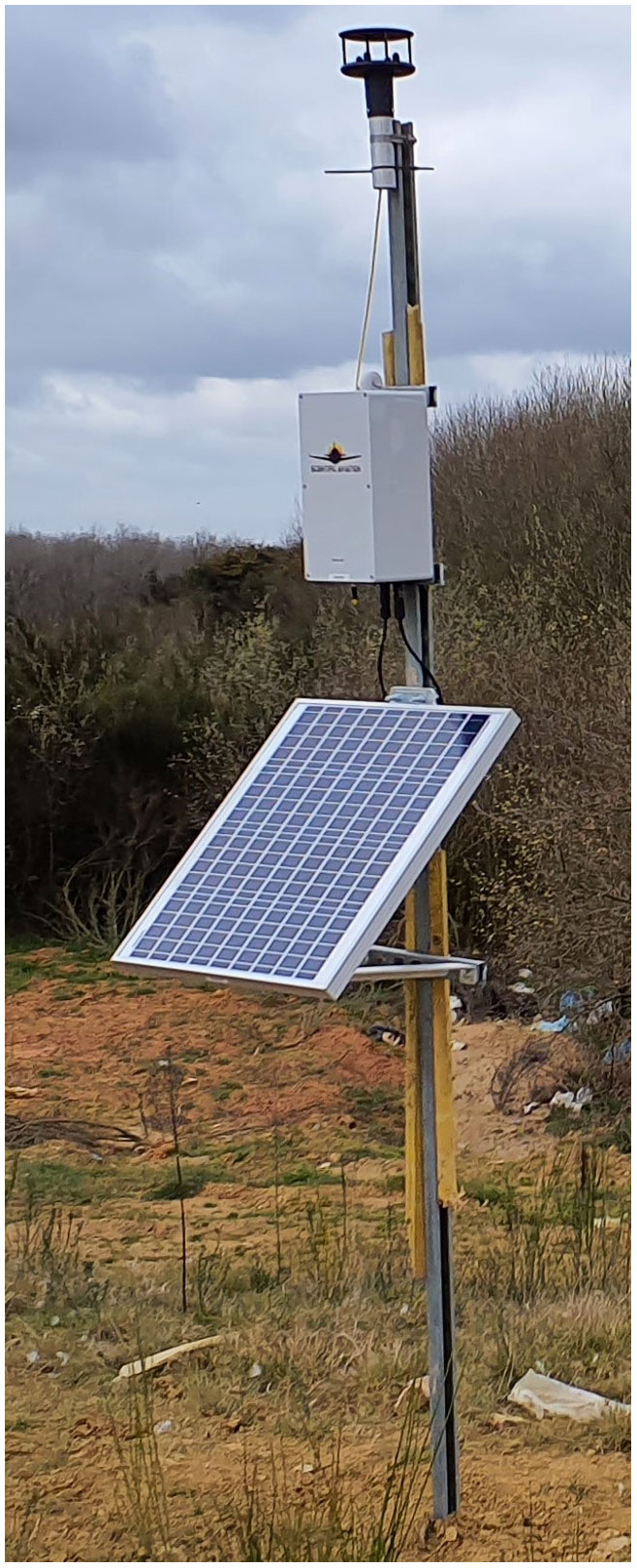
Figure 1 System A autonomous field logger (LSCE007) installed at the SUEZ Amailloux landfill site in March 2021 (see text for description). This system includes a two-dimensional anemometer.

2.3 Laboratory testing logging system

A bespoke laboratory logger was designed, with five sockets, to facilitate simultaneous Figaro testing (referred to hereafter as System B). The 0.1 dm³ cell has a glass exterior with a stainless-steel head (see Fig. 2), which was adapted from a filter (FS-2K-D, M&C TechGroup Germany GmbH, Ratingen, Germany). Each Figaro socket is connected in series with a high-precision 5.00 ± 0.05 kΩ load resistor (Vishay Intertechnology, Inc., Malvern, Pennsylvania, USA). This System B load resistance was selected to be identical to the load resistor in System A (which was determined by the System A manufacturer and beyond our control). 18-bit analogue-to-digital converter chips (MCP3424, Microchip Technology Inc., Chandler, Arizona, USA) measure 1 Hz V_d for each Figaro. This chip is ready-mounted onto an ADC Pi board (Apexweb Ltd, Swanage, Dorset, UK), which is connected to a Raspberry Pi 3B+ logging computer (Raspberry Pi Foundation, Cambridge, UK), using logging software similar to Rivera Martinez et al. (2021). A cable enters the top of the cell to provide connections between the Figaro circuit board and both the logging computer and ADC Pi board, which are outside the cell. The ADC Pi board is configured to sample at 16 bit, resulting in a 0.154 mV resolution, which, assuming a 5 kΩ Figaro resistance, is equivalent to an optimum resistance resolution of 0.6 Ω. A raw ADC Pi board V_s measurement is recorded, alongside raw Figaro V_d, to linearly calibrate the ADC Pi. Furthermore, a ground reference offset correction between the Figaro sensors and the ADC Pi board is applied to V_d.

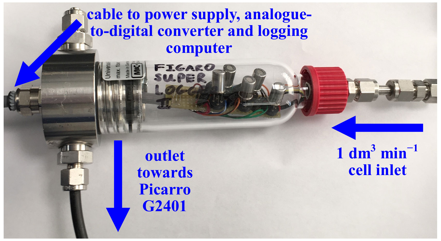
Figure 2 System B laboratory testing logging cell (logging computer and power supply not shown). Five Figaro sensors are plugged into the cell circuit board in this photograph.

Preliminary tests with a single power supply yielded unstable V_d measurements, as background activity on the logging computer influences total current draw. V_s also influences Figaro CH₄ sensitivity (see Appendix A). Therefore, the logging computer and Figaro power supplies are split, with a common ground, as suggested elsewhere (van den Bossche et al., 2017; Daugela et al., 2020). A high-precision power supply unit (T3PS23203P, Teledyne LeCroy Inc., Chestnut Ridge, New York, USA) provides Figaro power, with rated ripple and noise effects below ±1 mV (root mean squared) between 5 Hz and 1 MHz. A ±0.1 mV voltage standard deviation was observed when the power supply was tested with the ADC Pi board. The power supply unit also has a supply voltage read-back accuracy of at least 35 mV. Yet this rated accuracy does not affect our measurements, as the supply voltage setting was independently adjusted from the potential difference measured directly across the Figaro circuit board. This additionally corrects for voltage drop between the power supply unit and the Figaro sensors.

An SHT85 sensor measures System B temperature and relative humidity at 1 Hz inside the cell. In addition, the Figaro cell air outlet is fed through towards a Picarro G2401 gas analyser (Picarro, Inc., Santa Clara, California, USA), serving as an HPR. It records [CH₄], [H₂O], carbon monoxide mole fraction ([CO]) and [CO₂] at a maximum sampling frequency of 0.3 Hz, although the rate at which gas measurements are made decreases depending on the complexity of the gas mixture, with the Picarro G2401 designed to sample optimally in ambient gas conditions. The Picarro G2401 offers sampling with a high temporal stability (Yver Kwok et al., 2015), with a 0.2 Hz precision of less than ±0.001 ppm, ±0.0030 %, ±0.015 ppm and ±0.050 ppm for [CH₄], [H₂O], [CO] and [CO₂], respectively (Picarro, Inc., 2021). The Picarro G2401 streams data directly to the logging computer using a serial data connection; this simultaneous HPR logging eliminates time offset issues (i.e. if the Picarro G2401 clock is not synchronised with the System B clock), as the Picarro G2401 time stamp is not used. Any sensor response lag time between the System B sampling cell and the Picarro G2401 was measured and corrected for (typically a few seconds).

As Figaro sensors naturally operate in wet conditions, a dew-point generator (LI-610, LI-COR, Inc., Lincoln, Nebraska, USA) was employed during all System B testing. In addition, a variety of mass-flow controllers (Bronkhorst High-Tech B.V., AK Ruurlo, Netherlands) were utilised to produce various gas blends by combining different gas sources, all at a constant net 1 dm³ min⁻¹ flow rate. This is essential to maintain a consistent Figaro cooling effect inside the System B cell.

3 Sensor characterisation

3.1 Sensor gas response

Here we describe the general sampling strategy used to derive [CH₄]. According to the Figaro sensor characterisation strategy of van den Bossche et al. (2017) and Jørgensen et al. (2020), [CH₄] can be derived by comparing measured resistance to a baseline reference resistance (R_baseline) measured in the presence of a standard gas (Eugster and Kling, 2012). If this reference resistance is well-characterised to account for environmental changes (independent of gas composition), a gas derivation function (f) may be used to yield [CH₄], as in Eq. (2), where [CH₄]_baseline is the baseline reference [CH₄] in standard gas. This function is independent of environmental variables, as they are already incorporated in the reference resistance and thus cancel out. Therefore, this ratio is solely a function of gas enhancement.

$$\begin{array}{}\text{(2)}& f\left(\left(\right[{\mathrm{CH}}_{\mathrm{4}}]-[{\mathrm{CH}}_{\mathrm{4}}{]}_{\mathrm{baseline}}),\mathrm{\dots }\right)={\displaystyle \frac{R}{R_{\mathrm{baseline}}}}\end{array}$$

The f function may be dependent on various reducing or oxidising gases, though only CH₄ is explicitly included here for simplicity.

3.2 Choice of standard reference gas

In order to conduct repeatable testing, a reliable reference gas is first required. This gas must produce a consistent Figaro resistance response. Our initial candidate was gas from a zero-air generator (UHP-300ZA-S, Parker Hannifin Manufacturing Limited, Gateshead, Tyne and Wear, UK); this catalytic oven oxidises hydrocarbons and CO, resulting in a clean airstream containing 0.00 ppm [CH₄] and 0.00 ppm [CO], as recorded by the Picarro G2401. This reference gas was initially selected for testing due to enhanced Figaro environmental sensitivity expected in the absence of all reducing gases (Bastviken et al., 2020). Zero air was also employed as a reference gas by Jørgensen et al. (2020).

But before this zero-air source could be used as a standard gas in subsequent testing, it was important to verify that we could predict the resistance change under a [CH₄] transition from 0 to 2 ppm (ambient background), which would be a crucial step in working with zero air as a standard reference. This test was conducted with various gas samples containing the same 2 ppm [CH₄] from different sources, which were sampled with five sensors (LSCE001, LSCE003, LSCE005, LSCE007 and LSCE009) in System B. This System B testing was conducted in an air-conditioned laboratory. First, a cylinder containing 5 % [CH₄] in argon (P5-Gas ECD, Linde Gas AG, Höllriegelskreuth, Germany) was diluted with 99.996 % zero-air generator gas, targeting 2 ppm [CH₄], using mass-flow controllers for gas blending (discussed in Sect. 2.3). This was sampled twice. Next, a synthetic air cylinder containing 2 ppm [CH₄] (Deuste Gas Solutions GmbH, Schömberg, Germany) was sampled twice. Although this cylinder also contained 5000 ppm [CO₂], this is irrelevant in the context of Figaro resistance response (see Sect. 3.6). This was directly followed by sampling two ambient air sources once: ambient laboratory air from the room surrounding the instruments was sampled for 5 min, before finally sampling an ambient target gas cylinder which was filled with outdoor air from next to our laboratory building some months before. Ambient is defined here to be any natural air acquired from the surrounding environment.

A dew-point setting of 8 ^∘C was applied throughout this test, resulting in 0.970 ± 0.002 % [H₂O]. This was possible thanks to the closed-cell nature of System B with a fixed inlet, which allows precise gas samples to be delivered to the sensors with a constant [H₂O]. The sensors were allowed to stabilise in response to this [H₂O] setting for at least 24 h directly preceding the test until there was no noticeable resistance drift. This stabilisation period is essential, as Figaro sensors exhibit a delayed response to [H₂O] changes (see Appendix B).

Table 1 Fractional Figaro resistance decrease in response to different sources of 2 ppm methane mole fraction compared to zero-air generator gas. The final 120 s of each 2 ppm sampling period was used to derive these values. A zero-air reference resistance was derived by taking the average of all 120 s zero-air averages, preceding a 2 ppm transition.

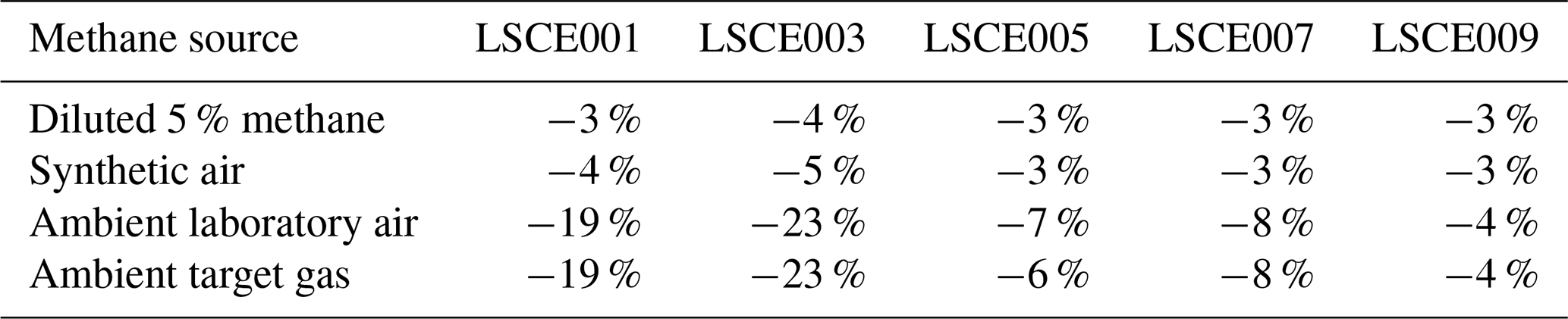
Results of this 2 ppm [CH₄] transition test are presented in Fig. 3. The Picarro G2401 recorded 2 ppm [CH₄] for all four gas samples, with consistently low [CO], which confirms the accuracy of diluting 5 % [CH₄] in argon using mass-flow controllers. However, Figaro resistance decrease varied considerably (see Table 1 for fractional decrease values). Resistance drop (compared to zero-air generator gas) when sampling both ambient target gas and ambient laboratory air was smaller (on average 4 % for all five sensors) than when sampling synthetic air and diluted 5 % [CH₄] (on average 12 % for all five sensors), although there was considerable variability between the different sensors (see Table 1). This suggests that there may be one (or many) additional species in ambient air, causing an unexpectedly high Figaro resistance drop. Such a substance may be absent in synthetic air and combusted by the zero-air generator. However, identifying such species remains a challenge (see Sect. 5.2 for discussion), with us unable to identify any obvious alternative ambient reducing candidates from previous Figaro testing work. Moreover, the consistent resistance drops for both synthetic 2 ppm [CH₄] and zero air blended with 0.004 % of 5 % [CH₄] suggest that synthetic 2 ppm [CH₄] contains no reducing contaminants.

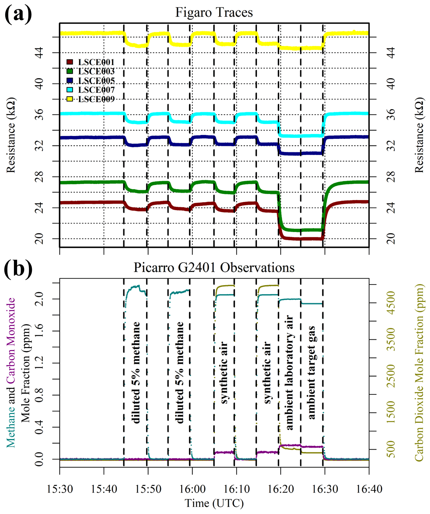
Figure 3 (a) Measured resistance for five Figaro sensors in System B (coloured dots; see legend) under exposure to various sources of 2 ppm methane mole fraction (all compared to gas from a zero-air generator). (b) Corresponding Picarro G2401 mole fraction observations, with annotations indicating the sampled 2 ppm methane source. Areas not annotated correspond to gas from the zero-air generator. Methane (dark cyan) and carbon monoxide (dark magenta) mole fraction measurements are plotted on the left-hand axis. Carbon dioxide (dark yellow) mole fraction measurements are plotted on the right-hand axis.

Although this test infers the presence of an interfering substance in ambient natural air (both target gas and laboratory air), it is important to verify that the zero-air generator itself is not a source of such components. It is also useful to test whether different synthetic air cylinders (filled at different times) from the same supplier (Deuste Gas Solutions GmbH) behave in the same way compared to zero-air generator gas. All synthetic air cylinders from this supplier contain a natural balance of nitrogen, oxygen and argon, to which trace quantities of other gases are added. System B was used to sample a synthetic 50 ppm [CH₄] cylinder filled in 2019 (old), a synthetic 50 ppm [CH₄] cylinder filled in 2021 (new), a synthetic zero-air cylinder filled in 2014 (old) and a synthetic zero-air cylinder filled in 2021 (new), which were all sampled twice. Four sensors were tested (LSCE002, LSCE004, LSCE006 and LSCE008) at a fixed dew point, resulting in 0.652 ± 0.010 % [H₂O] for this test. A sufficient [H₂O] stabilisation period preceded this test.

Figure 4 shows Figaro and HPR observations from this test. The two synthetic 50 ppm [CH₄] cylinders (old and new) both produced identical resistance decreases compared to gas from the zero-air generator when filled 2 years apart. This suggests that the quality of synthetic 50 ppm [CH₄] cylinders is consistent and that CH₄ is the dominant reducing species in these cylinders. The second part of the test shows that synthetic zero air has a negligible effect on Figaro resistance compared to gas from the zero-air generator. Though synthetic zero air causes a small resistance variability (particularly for LSCE006; see Fig. 4), this is insignificant in the context of the resistance decrease values presented in Table 1 for different 2 ppm [CH₄] sources. This consistency in zero-air resistance response suggests that the zero-air generator successfully burns Figaro-sensitive species. This supports the conclusions derived from Fig. 3 that there may be an additional reducing substance in natural air that is otherwise absent in zero air from multiple sources (both synthetic and from the zero-air generator).

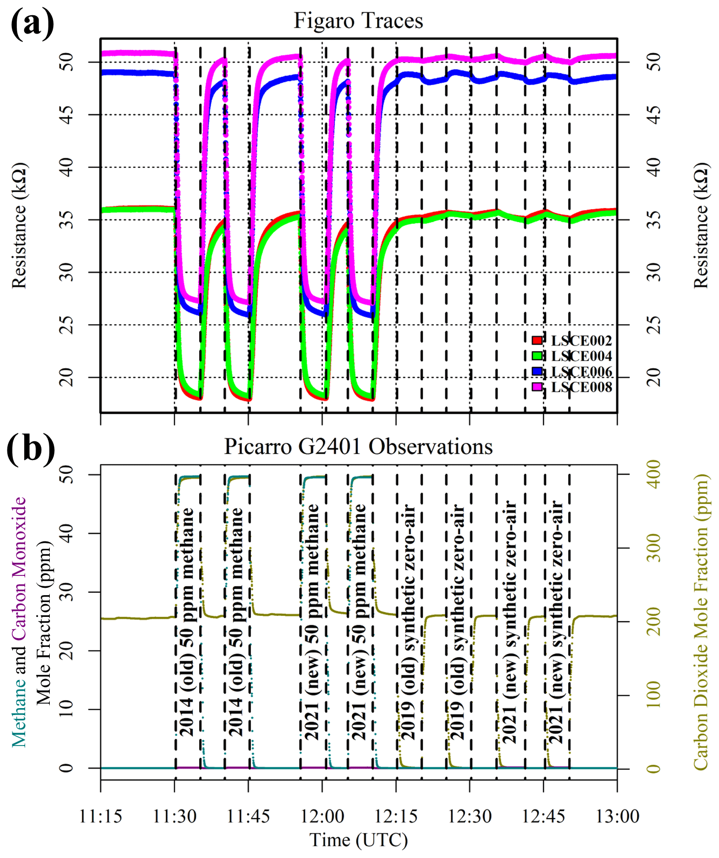
Figure 4 (a) Measured resistance for four Figaro sensors in System B (coloured dots; see legend) under exposure to two sources of 50 ppm methane mole fraction and two sources of synthetic zero air (all compared to gas from a zero-air generator). (b) Corresponding Picarro G2401 mole fraction observations, with annotations indicating the synthetic cylinder type. Areas not annotated correspond to gas from the zero-air generator. Methane (dark cyan) and carbon monoxide (dark magenta) mole fraction measurements are plotted on the left-hand axis. Carbon dioxide (dark yellow) mole fraction measurements are plotted on the right-hand axis.

To summarise, these two tests imply that zero air (either synthetic or from a zero-air generator) is an unsuitable standard reference gas. Figaro resistance is abnormally high in zero air due to the possible absence of (non-CH₄) interfering reducing species otherwise present in ambient air. The fact that the resistance drop in ambient laboratory air was almost identical to the resistance drop in ambient target gas (filled some months before) suggests that any unidentified background reducing species are stable, with a long lifetime. Elsewhere, Jørgensen et al. (2020) found that a laboratory calibration conducted with zero air could not be applied to ambient air sampling, which required its own calibration (attributing this to power supply issues). Additionally, van den Bossche et al. (2017) found that applying a calibration made in synthetic air to ambient air resulted in larger sensor disparity compared to an HPR. They attributed this to ±2 % oxygen mole fraction ([O₂]) variability in their synthetic air source (van den Bossche et al., 2017); however, our oxygen test (see Sect. 3.7) shows that this is unlikely and an interfering species was probably responsible. Yet, during our tests, we were unable to identify such interfering species from our HPR and there are no other obvious reducing candidates in ambient air (see Sect. 5.2 for discussion). The oxidising capacity of air is unlikely to vary, as surface [O₂] is nearly constant. Furthermore, Collier-Oxandale et al. (2018) observed no ozone sensitivity for the similar Figaro TGS 2600 sensor.

Therefore, to incorporate this natural background effect into any subsequent models or analysis, natural ambient air should be employed as a standard gas instead of zero air, assuming that the ambient air background composition remains consistent in various characterisation tests. Although natural air contains both CH₄ and CO, their variability is typically small when not in the close vicinity of emission sources. Hence, all subsequent testing assumes an ambient 2 ppm [CH₄] background.

3.3 Reference resistance characterisation

Having selected natural ambient air as a standard gas, the next step is to characterise a standard 2 ppm [CH₄] baseline reference resistance (R_2 ppm) in response to environmental variables (independent of gas composition), which dominate Figaro performance (Eugster and Kling, 2012; Collier-Oxandale et al., 2019; Rivera Martinez et al., 2021; Furuta et al., 2022). The most important environmental factors (discussed in Sect. 1) are temperature and [H₂O] (Eugster et al., 2020), which were characterised using a large environmental chamber (UD500 C, Angelantoni Test Technologies Srl, Massa Martana, Italy) to simultaneously test five System A loggers. The chamber was slowly replenished (at less than 0.5 dm³ min⁻¹) to avoid the accumulation of waste gas species, such as CO, which can be formed due to some incomplete CH₄ combustion on the Figaro sensor surface (Glöckler et al., 2020). Rather than using a solar panel, each System A battery was connected directly to a battery charger to maintain a stable battery voltage and hence a stable Figaro supply voltage. System A data were remotely accessed by connecting the cellular board inside each enclosure to an antenna outside the environmental chamber. The Picarro G2401 HPR continuously sampled inside the chamber during testing. All System A data were interpolated to the shorter Picarro G2401 time stamp.

Chamber testing was conducted across a temperature and [H₂O] range expected in the field, as suggested elsewhere (Barsan et al., 2007), to optimise time resources with limited chamber access. [H₂O] levels of 0.4 %, 0.7 %, 1.0 %, 1.4 % and 1.9 % were targeted by adjusting relative humidity inside the chamber, according to the temperature setting. Relative humidity control was essential in this test, as residual liquid water evaporated from the chamber walls with a temperature setting increase. Following each new [H₂O] change, the chamber was first given one 7 h adjustment period to augment [H₂O] stabilisation, as required in response to sharp [H₂O] changes (see Appendix B). Next, at least four different temperature settings were sampled at each [H₂O] level in 4 h intervals (including time for each temperature ramp). Finally, temperature was varied in 8 h sampling intervals at the same fixed [H₂O] level. Then the entire process was repeated at a different targeted [H₂O].

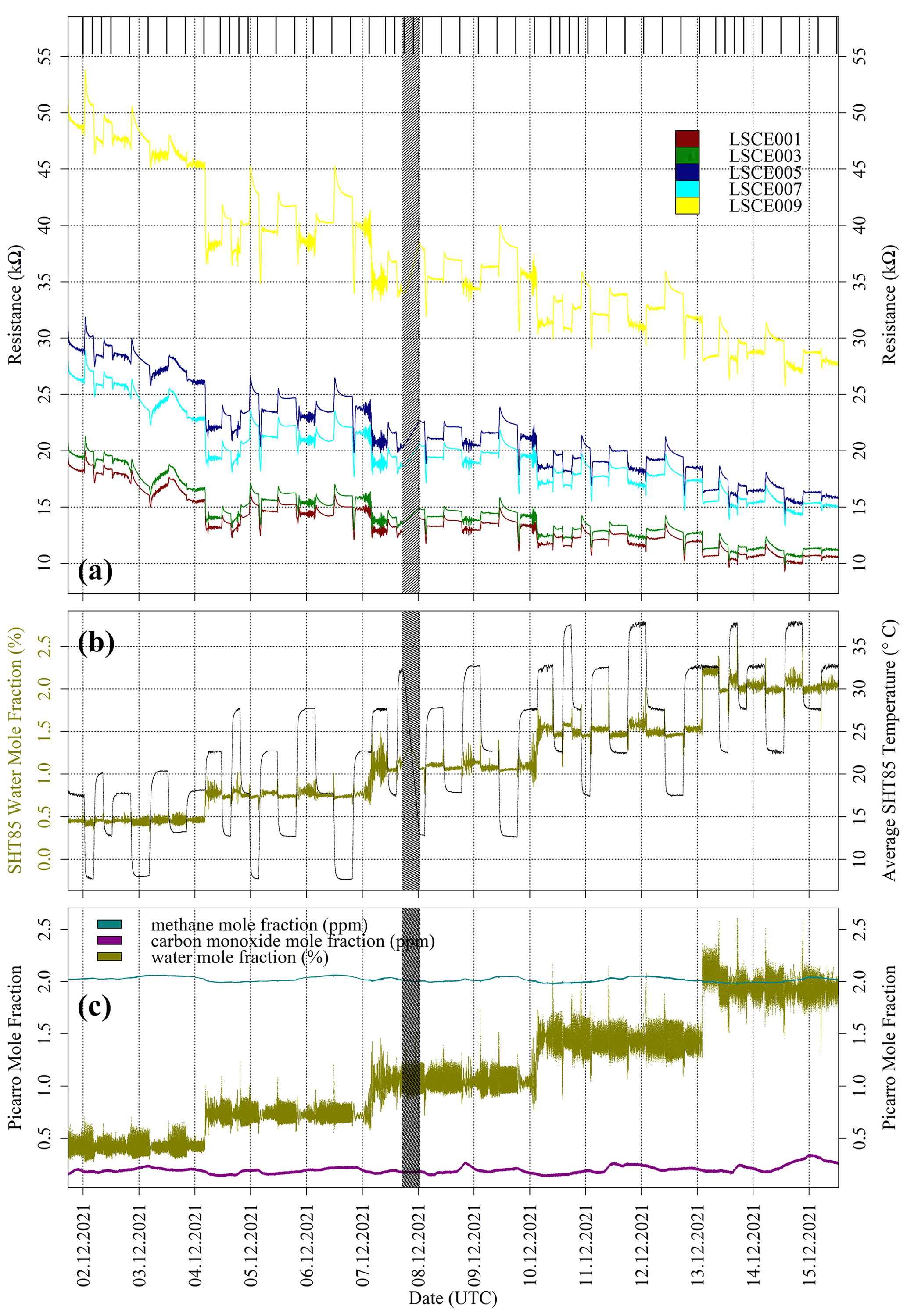
Figure 5 (a) Resistance for five Figaro sensors, sampling inside the environmental chamber (coloured dots; see legend). The black bars at the top of the plot indicate periods used to derive 30 min averages for each sampling period. The shaded area indicates a data transmission gap. (b) Derived SHT85 water vapour mole fraction (dark yellow dots) averaged from all five System A boxes plotted against the left-hand axis (see text for derivation details) and measured SHT85 temperature averaged from all five System A boxes (black dots) plotted on the right-hand axis. (c) Picarro G2401 measurements from inside the chamber. Methane (dark cyan) and carbon monoxide (dark magenta) mole fractions are plotted in parts per million; the water (dark yellow) mole fraction is plotted in percent.

Chamber observations from each System A logger are presented in Fig. 5, alongside corresponding HPR measurements. There was a data transmission gap between 17:14 UTC on 7 December 2021 and 00:46 UTC on 8 December 2021. Average SHT85 T_A measurements and derived SHT85 [H₂O] values from all five System A boxes are also shown in Fig. 5. [H₂O] values were derived using SHT85 T_A and relative humidity measurements from inside each System A enclosure, where saturation vapour pressure was derived using the Tetens equation, given by Murray (1967), and pressure was assumed to be 10⁵ Pa, which can be simplified to Eq. (3). M₁ and M₂ are equal to 17.2693882 and 35.86 K, respectively, over water and 21.8745584 and 7.66 K, respectively, over ice.

$$\begin{array}{}\text{(3)}& \left[{\mathrm{H}}_{\mathrm{2}}\mathrm{O}\right]=\mathrm{relative}\mathrm{humidity}\cdot \mathrm{0.000061078}\cdot e^{M_{\mathrm{1}}\cdot \frac{\left(T_{\mathrm{A}}-\mathrm{273.16}\right)}{T_{\mathrm{A}}-M_{\mathrm{2}}}}\end{array}$$

The average standard deviation in T_A and [H₂O] was 0.14 ± 0.13 ^∘C and 0.0089 ± 0.0063 %, respectively, between the five System A logging systems as a function of time, showing that the boxes were exposed to almost identical conditions for the duration of this experiment.

Despite our efforts to maintain a fixed [H₂O] level during temperature variations, there was a sharp [H₂O] change at each temperature transition with periodic [H₂O] fluctuations (see Fig. 5), as the environmental chamber constantly worked to rectify itself to achieve its target environmental settings. [H₂O] therefore fluctuated both above and below a central point periodically, following an initial larger variability associated with each pre-programmed step. Although many hours of stable sampling are required for sufficient Figaro stabilisation following a [H₂O] step change (see Appendix B), regular periodic fluctuations in [H₂O] should cancel each other out over a sufficient averaging period, as the resistance decay behaviour occurs in both a positive and negative direction. Nevertheless, Fig. 5 shows that 4 h of sampling was insufficient for resistance stabilisation following the initial step change. Therefore, these 4 h sampling periods were not used (thus conveniently avoiding the data transmission gap). Instead, 30 min averages were taken towards the end of each 8 h sampling period, ranging between 10 and 47 kΩ for the five sensors. Figure 5 shows that despite [H₂O] variability resulting in noisy resistance measurements, there was no overall upwards or downwards resistance drift after 8 h of sampling, with small resistance variations (due to direct [H₂O] fluctuations) superimposed on a larger water stabilisation effect.

These chamber averages showed that [H₂O] is the dominant factor influencing R_2 ppm, as observed in other work (Bastviken et al., 2020; Rivera Martinez et al., 2021), exhibiting a linearly decreasing relationship. Therefore, Eq. (4) was proposed to model R_2 ppm in the environmental chamber. This equation is analogous to Eq. (2), where R_2 ppm is specifically used in place of a general R_baseline value.

$$\begin{array}{}\text{(4)}& R_{\mathrm{2}\mathrm{ppm}}=A\cdot \left(\mathrm{1}-\left(\left[{\mathrm{H}}_{\mathrm{2}}\mathrm{O}\right]\cdot \left(B-\left(T_{\mathrm{A}}\cdot C\right)\right)\right)-\left(T_{\mathrm{A}}\cdot D\right)\right)\end{array}$$

A is a baseline reference resistance offset in kΩ, B is a water correction coefficient in %⁻¹, C is a temperature–water correction coefficient in kK⁻¹ %⁻¹ and D is temperature correction coefficient in kK⁻¹, where “%” is a percentage water vapour mole fraction. [H₂O] here represents a derived value from the SHT85 inside each System A enclosure.

Table 2 Equation (4) model parameters for five System A enclosures derived from 30 min averages (of 8 h testing windows), whilst sampling natural ambient air in the environmental chamber. The R² and RMSE are given for each model fit, and the RMSE is given as a fraction of R_2 ppm at 25 ^∘C T_A and 1 % [H₂O] for each sensor.

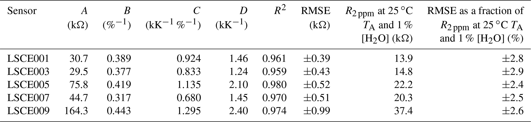
Table 3 AIC and BIC scores for simplified variations of the Eq. (4) model for five System A enclosures derived from 30 min averages (of 8 h testing windows), whilst sampling natural ambient air in the environmental chamber.

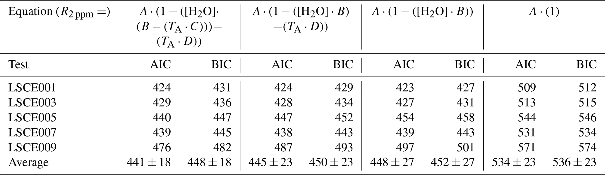
A non-linear regression was applied between R_2 ppm, T_A and [H₂O] from all 30 min averages from the 8 h sampling periods for each sensor. It is worth noting that any empirical model parameters derived from this test are specific to the logging system in which they were derived, as flow dynamics in each logging system are different, resulting in a different Figaro cooling effect. Furthermore, T_A is specifically influenced by the temperature gradient between the Figaro sensor and the point of temperature measurement in System A. Model results are presented in Fig. 6 and corresponding model coefficients in Table 2. As Eq. (4) contains four free parameters, with a limited number of sampling data points, we evaluated the suitability of parameterisation. An Akaike information criterion (AIC) and Bayesian information criterion (BIC) score was derived for simplified variations of Eq. (4), with one, two and three free parameters. Results are presented in Table 3, where a lower AIC and BIC score represents a better compromise, providing a good model fit without over-parameterisation. The results in Table 3 show that, on average, the full version of Eq. (4) with four free parameters results in the lowest AIC and BIC score, supporting our four-parameter approach.

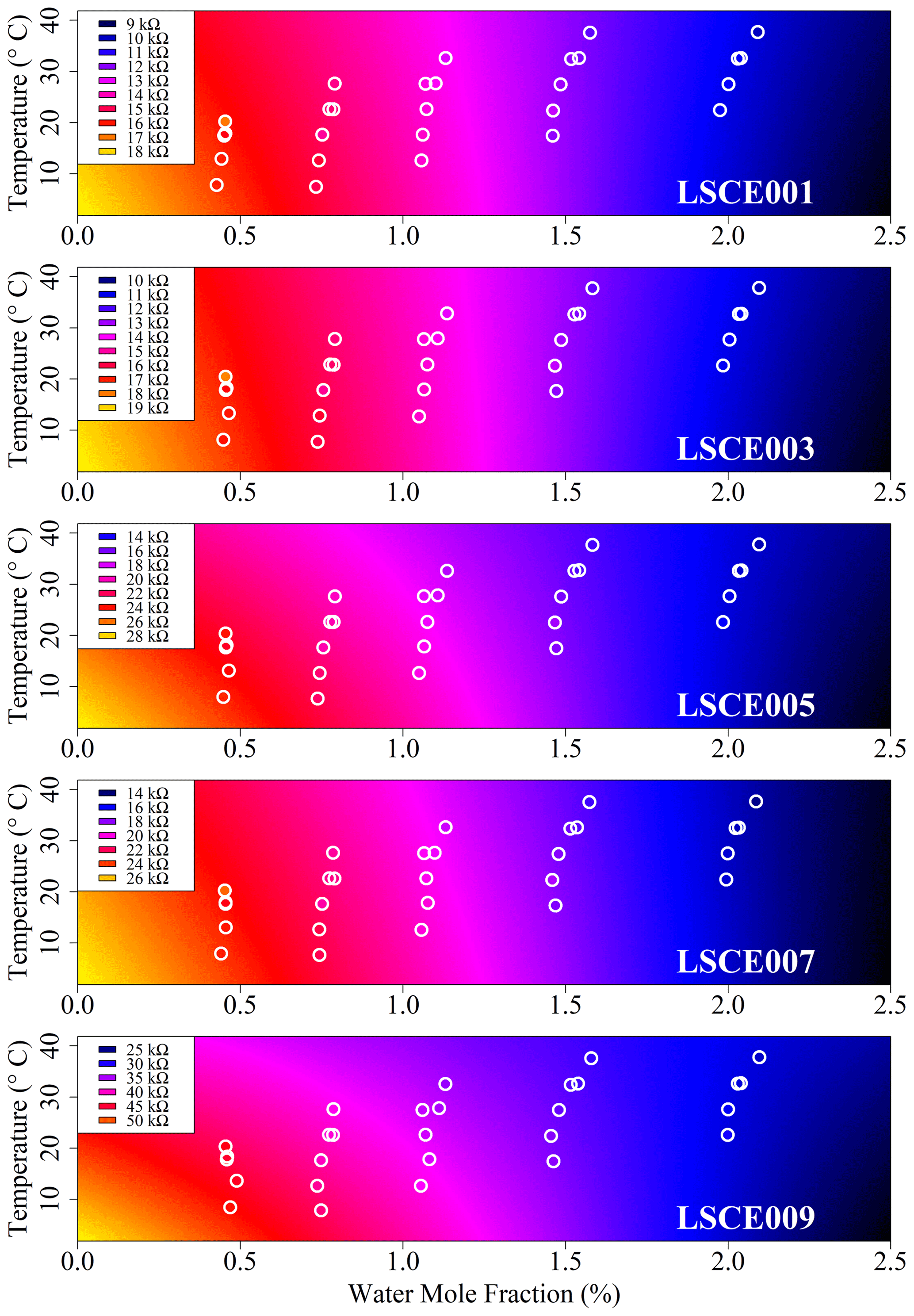
Figure 6 Modelled reference resistance at 2 ppm methane mole fraction (standard gas) for LSCE001, LSCE003, LSCE005, LSCE007 and LSCE009 (coloured background). Points inside white circles represent 30 min measured resistance averages. Each plot has a unique colour scale (see legend).

Having selected the four-parameter model given by Eq. (4), the RMSE in R_2 ppm when modelling environmental chamber sampling was derived and is provided in Table 2, spanning between ±0.4 and ±1.0 kΩ. For all five sensors this represents less than ±3 % fractional uncertainty in R_2 ppm at 25 ^∘C T_A and 1 % [H₂O] (assuming that the sensor has reached a stable level in response to [H₂O] changes). This means that the Eq. (4) model can predict Figaro resistance to within ±3 % in standard conditions based solely on temperature and [H₂O], when sampling natural air containing 2 ppm [CH₄]. This low model error suggests that Eq. (4) provides good temperature and [H₂O] constraints to R_2 ppm. Furthermore, an R² of 0.97 ± 0.01 for the five model fits illustrates the suitability of Eq. (4) to characterise R_2 ppm with respect to environmental conditions (see Table 2 for values). By accurately modelling R_2 ppm as a first step, this resistance value can then be used to derive [CH₄] from its change in the presence of enhanced levels of CH₄.

3.4 Methane characterisation

In order to derive a Figaro CH₄ response function, the effect of adding CH₄ to standard gas (natural ambient air) was characterised by testing five Figaro sensors (LSCE001, LSCE003, LSCE005, LSCE007 and LSCE009) using System B. Ambient laboratory air (which naturally contains 2 ppm [CH₄]) was blended with gas from a cylinder containing 5 % [CH₄] in argon (P5-Gas ECD, Linde Gas AG) in 15 min intervals from 2 ppm (pure ambient laboratory air) up to a target level of 1000 ppm [CH₄] using a pre-programmed mass-flow controller flow script (see Sect. 2.3 for details). When compared to natural ambient air, this maximum 1000 ppm [CH₄] gas blend has an argon mole fraction enhancement of 145 % and an oxygen and nitrogen mole fraction diminution of 1.44 %. This 1000 ppm level represents a realistic upper limit on typical [CH₄] enhancements expected in the vicinity of most CH₄ sources, such as large leaks from oil and gas extraction infrastructure. This high upper [CH₄] limit also facilitates better sensor characterisation over an extended range. Following at least 1 h of ambient laboratory air sampling, [CH₄] was gradually raised up to its maximum level and then lowered, stepwise, in three cycles. After each cycle, ambient laboratory air was sampled for 1 h to provide an R_2 ppm reference. This approach is similar to that of Jørgensen et al. (2020), who instead transitioned back to their standard gas following each individual gas enhancement. Throughout our test, an 8 ^∘C dew-point setting was applied, which was sampled from at least 24 h in advance to facilitate the necessary water stabilisation (see Appendix B).

Full Figaro resistance results are presented in Fig. 7. Figure S3 in the Supplement provides an example of a single [CH₄] transition for LSCE009, which shows that the final 2 min is a suitable representation of stable Figaro resistance thanks to efficient cell flushing, unlike a long cell residence time observed in other work (Rivera Martinez et al., 2023). Figure S3 also shows that there is little noise in System B Figaro measurements. Therefore, a 2 min resistance average was derived at the end of each 15 min sampling period (highlighted in Fig. 7). Although a longer averaging period could have been used, we decided to minimise this duration to 2 min for maximal possible stability. A specific R_2 ppm reference baseline was then derived for this test by fitting a second-order polynomial to the final 15 min of each 1 h standard (ambient laboratory air) sampling period, except the first period, for which 45 min of sampling was instead used (see Fig. 7). R_2 ppm was not derived from Eq. (4) in this test, as derived empirical Eq. (4) model parameters from Sect. 3.3 are only valid in System A under specific System A flow dynamics and with a specific System A T_A measurement. By instead using a polynomial R_2 ppm fit, any reference resistance variability was incorporated into R_2 ppm during the test, which may occur due to small environmental changes. In any case, temperature and [H₂O] both remained stable: [H₂O] was on average 1.002 ± 0.001 % during R_2 ppm sampling periods according to the Picarro G2401 HPR, and System B temperature was on average 34.2 ± 0.2 ^∘C according to the SHT85 inside the System B cell.

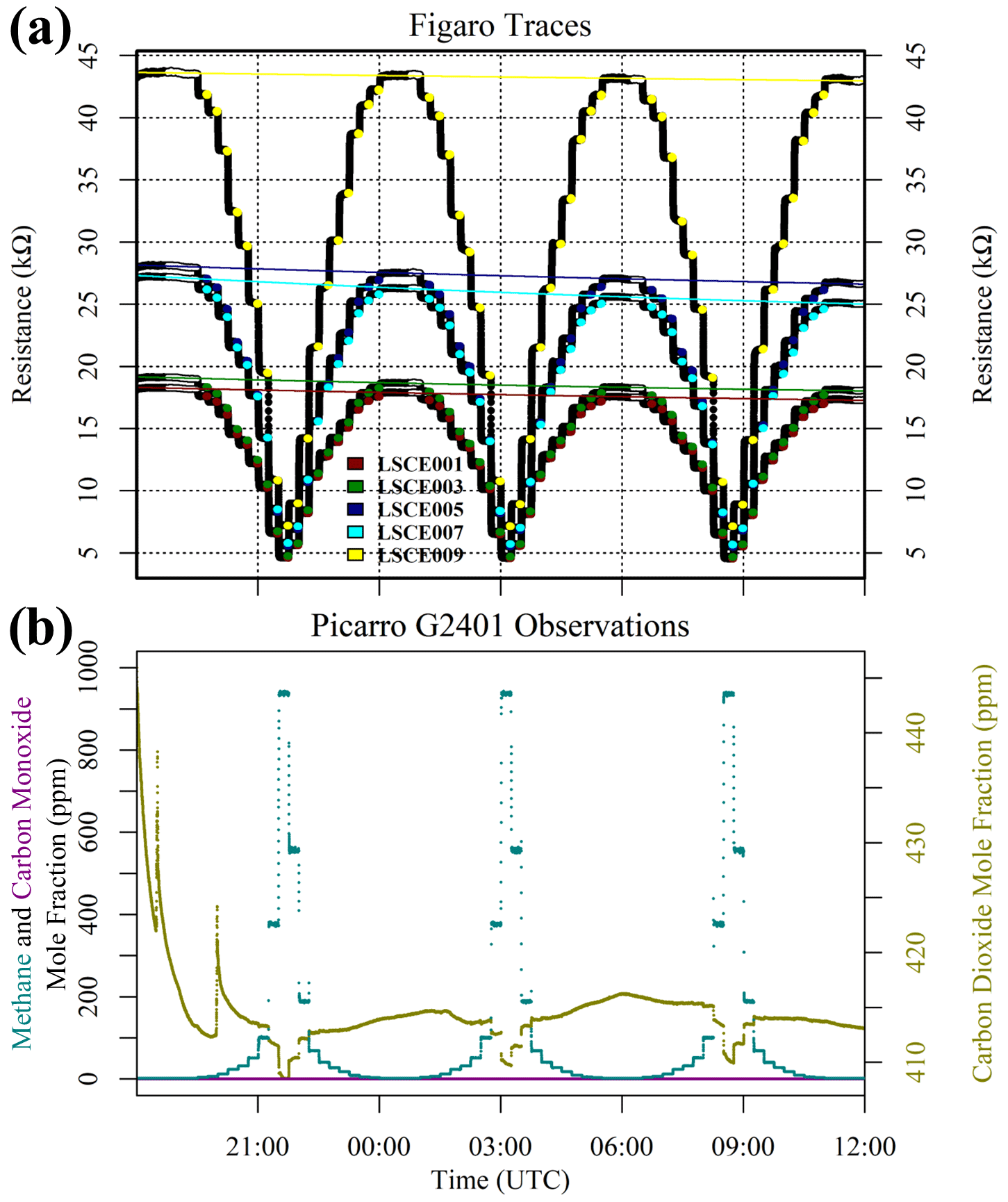
Figure 7 (a) Measured resistance for five Figaro sensors (black dots) under exposure to various methane mole fraction intervals up to 1000 ppm. Highlighted coloured dots represent 2 min periods used to derive average resistance values for each methane step (see legend for corresponding sensor colours). White-highlighted dots indicate periods used to derive standard gas reference resistances for each sensor, and coloured lines show respective polynomial reference resistance fits. (b) Corresponding mole fraction observations from the Picarro G2401. Methane (dark cyan) and carbon monoxide (dark magenta) mole fraction measurements are plotted on the left-hand axis. Carbon dioxide (dark yellow) mole fraction measurements are plotted on the right-hand axis. Carbon dioxide measurements become unreliable at a high methane mole fraction due to spectral overlap.

For each 2 min Figaro resistance average, corresponding Picarro G2401 [CH₄] averages were derived. Wet [CH₄] is used here and throughout this paper to minimise errors associated with the internal Picarro G2401 water correction, especially at higher [CH₄], where spectral overlap becomes more prominent and [H₂O] measurements become less reliable. For [CH₄] of over 100 ppm, [CH₄] was instead derived from the mass-flow controller setting, as the Picarro G2401 is less precise at high [CH₄]. Water was then reintroduced into these dry [CH₄] estimates. The ratio between each measured resistance average and its corresponding polynomial R_2 ppm estimate was then deduced and plotted against its respective [CH₄] value in Fig. 8.

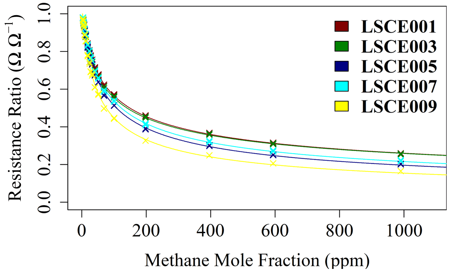
Figure 8 The ratio between each 2 min average Figaro resistance (from 15 min sampling intervals) and its corresponding reference resistance estimate (crosses), plotted against methane mole fraction for five Figaro sensors (see legend for respective colours). A model fit for each sensor (coloured lines) is plotted according to Eq. (6).

Figure 8 suggests that the resistance ratio follows a power-law decay behaviour, whereby the resistance ratio slowly tends towards zero as [CH₄] enhancement (above the 2 ppm standard) tends to infinity. However, a simple power-law fit cannot be used here: when mole fraction enhancement is equal to zero (i.e. when [CH₄] is equal to the 2 ppm standard), the resistance ratio must be equal to unity (i.e. R_2 ppm must equal R). Therefore, Eq. (5) is proposed, where 1 is added to the CH₄ gas term to satisfy this requirement.

$$\begin{array}{}\text{(5)}& \begin{array}{rl}R=& R_{\mathrm{2}\mathrm{ppm}}\left(T_{\mathrm{A}},\left[{\mathrm{H}}_{\mathrm{2}}\mathrm{O}\right]\right)\cdot {\left(\mathrm{1}+\left({\displaystyle \frac{\left[{\mathrm{CH}}_{\mathrm{4}}\right]-\mathrm{2}\mathrm{ppm}}{a}}\right)\right)}^{-\mathit{\alpha }}\\ & \cdot \prod _g{\left(\mathrm{1}+\left({\displaystyle \frac{\left[M_g\right]-[M{]}_{{\mathrm{0}}_g}}{c_g}}\right)\right)}^{-{\mathit{\gamma }}_g}\end{array}\end{array}$$

Here, a is the characteristic methane mole fraction and α is the methane power. Other reducing gases (g) may be included in Eq. (4) depending on sampling conditions, where [M] is the mole fraction of g, [M]₀ is the standard mole fraction of g (in ambient air), c is the characteristic mole fraction of g and γ is the power of g. Equation (5) is a general equation which allows any potential reducing gases to be incorporated in Figaro resistance response. However, for a more specific case when [M] is equal to [M]₀, as in standard gas, these multiplicative terms tend to unity and can be ignored from Eq. (5), thus simplifying to Eq. (6).

$$\begin{array}{}\text{(6)}& R\approx R_{\mathrm{2}\mathrm{ppm}}\left(T_{\mathrm{A}},\left[{\mathrm{H}}_{\mathrm{2}}\mathrm{O}\right]\right)\cdot {\left(\mathrm{1}+\left({\displaystyle \frac{\left[{\mathrm{CH}}_{\mathrm{4}}\right]-\mathrm{2}\mathrm{ppm}}{a}}\right)\right)}^{-\mathit{\alpha }}\end{array}$$

Thus, rather than deriving c and γ for each potential reducing gas, Eq. (6) only focuses on a single variable gas (CH₄, in this case), which is responsible for most resistance variability.

Table 4 Equation (6) methane model parameters for five Figaro sensors, with the R² and RMSE for each model fit. Inverted methane mole fraction RMSE values are also given over the full 1000 ppm range and with a 28 ppm threshold. The expected ratio between measured resistance and R_2 ppm is also provided for a 1 and 48 ppm [CH₄] enhancement above the 2 ppm background.

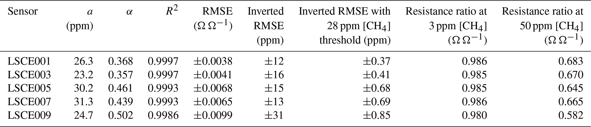
This model fits the System B measurements of resistance ratio (i.e. measured resistance averages divided by their corresponding polynomial R_2 ppm estimates) from the CH₄ characterisation test very well (see Table 4 for a and α for the five tested sensors), which justifies our 2 min averaging experimental approach. This model fit yields an RMSE resistance ratio of no more than ±1 % Ω Ω⁻¹ and an R² of 0.9993 ± 0.0005 for the five sensors. This means that over a 1000 ppm [CH₄] range, the ratio between measured Figaro resistance and standard reference resistance can be predicted to within ±1 %, thus allowing [CH₄] estimates to be derived by comparing measured resistance to R_2 ppm. Equation (6) was also inverted to make [CH₄] the subject. Using the same original fitting parameters provided in Table 4, this revealed an inverted [CH₄] RMSE of no more than ±31 ppm for the model fit over the full 1000 ppm range (see Table 4 for individual values). Applying a [CH₄] threshold reduced this uncertainty further, as [CH₄] is more accurate at lower [CH₄], where there are more data points. Taking [CH₄] values of 28 ppm and lower (nine targeted [CH₄] levels) and using the same fitting parameters from the extended [CH₄] range resulted in a reduced inverted [CH₄] RMSE uncertainty of no more than ±0.85 ppm. Though it is possible to derive better fitting parameters in this reduced [CH₄] range, the extended [CH₄] range permits better characterisation of the natural power decay behaviour. Furthermore, characterising only small [CH₄] enhancements limits the model to such circumstances; this may be desirable in cases in which there is certainty that sampled [CH₄] enhancements will remain low.

Although there is a good CH₄ model fit for the extended [CH₄] range, in practice, [CH₄] can only be derived from the ratio between measured resistance and R_2 ppm. The resistance ratio for a 1 ppm enhancement above the background (to 3 ppm [CH₄]) would be between 0.980 and 0.986 Ω Ω⁻¹ for the five tested sensors, while the resistance ratio for a 48 ppm enhancement above the background (to 50 ppm [CH₄]) would be between 0.582 and 0.683 Ω Ω⁻¹ (see Table 4 for individual values). This makes small [CH₄] enhancements difficult to detect; a transition from 2 to 3 ppm [CH₄] results in a resistance drop of as little as 1 %. Thus, [CH₄] estimation using Eq. (6) requires good modelled R_2 ppm estimates (from Sect. 3.3) in order to derive a reliable resistance ratio.

3.5 Carbon monoxide influence

[CO] can vary in natural ambient air depending on nearby pollution (e.g. petrol and diesel cars) but is typically of the order of 10⁻¹ ppm. As CO is a potent reducing gas, the importance of CO variations within standard ambient air was tested with four sensors (LSCE002, LSCE004, LSCE006 and LSCE008) in System B. Figaro resistance at 0.1 ppm [CO] was compared to a 0.0 ppm [CO] standard baseline reference (with only CO removed). An ambient target gas cylinder filled with outside air (2 ppm [CH₄] and 0.15 ppm [CO]) was split into two gas streams: one stream was directly from the cylinder and the other stream passed through a chemical CO scrubber (Sofnocat 514, Molecular Products, Limited, Harlow, Essex, UK). The 0.0 ppm [CO] reference was first sampled for at least 1 h. Then, 0.1 ppm [CO] was sampled in four 15 min intervals. Each 0.1 ppm interval was followed by 15 min sampling the 0.0 ppm [CO] reference. A fixed 8 ^∘C dew-point setting was applied and a sufficient [H₂O] stabilisation period preceded this test.

Figaro resistances and corresponding HPR measurements are presented in Fig. 9. [CH₄] remained fixed at 2 ppm throughout this test, allowing us to assess the independent influence of CO on Figaro resistance in the standard gas (natural ambient air). A 5 min average was taken from the end of each 15 min 0.1 ppm [CO] sampling period (highlighted in Fig. 9). Although Fig. 9 shows that the sensors stabilise relatively quickly in response to CO, we decided to err on the side of caution and to limit the averaging period to the final 5 min out of 15 min based on the observed resistance delay in the CH₄ test (see Fig. S3). A baseline reference was then derived by fitting a second-order polynomial to the final 5 min of each 15 min reference (0.0 ppm [CO]) sampling period, except the first period for which 45 min was used (see Fig. 9). [H₂O] was on average 0.983 ± 0.001 % during these reference sampling periods according to the Picarro G2401, and System B temperature was on average 31.3 ± 0.1 ^∘C according to the SHT85 sensor inside the cell.

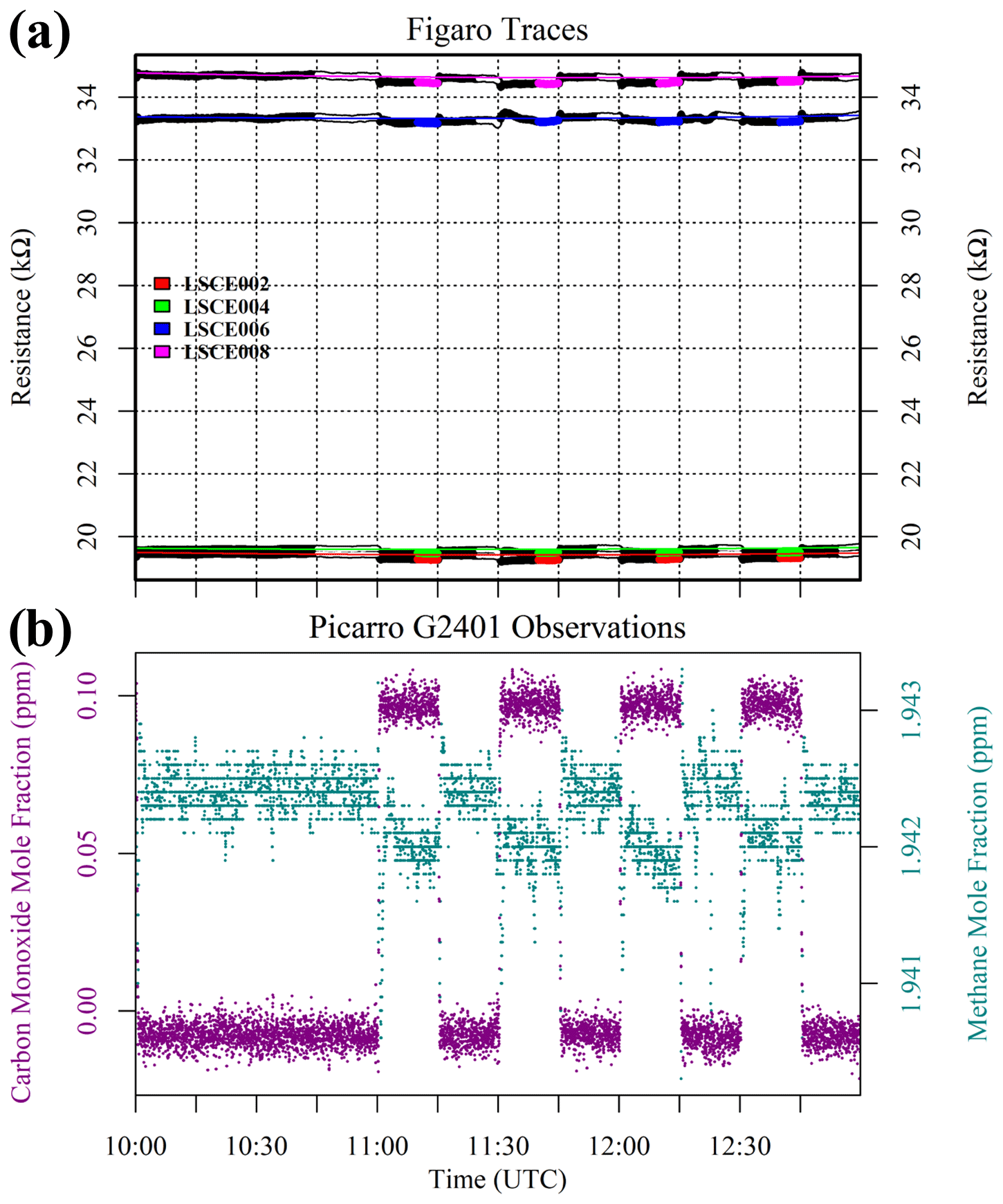
Figure 9 (a) Measured resistance for five Figaro sensors (black dots) when varying the carbon monoxide mole fraction in standard gas between 0.0 and 0.1 ppm. Highlighted coloured dots represent 5 min periods used to derive an average resistance for each 0.1 ppm interval (see legend for corresponding sensor colours). White-highlighted dots indicate periods used to derive 0 ppm reference resistances for each sensor, and coloured lines show respective polynomial reference resistance fits. (b) Corresponding Picarro G2401 observations. Methane (dark cyan) mole fraction measurements are plotted on the left-hand axis, and carbon monoxide (dark magenta) mole fraction measurements are plotted on the right-hand axis.

The resistance ratio between each 5 min 0.1 ppm [CO] average and its corresponding modelled reference (0.0 ppm [CO]) resistance was derived. Four individual resistance ratios were acquired and then averaged for each sensor: 0.9922 ± 0.0006 Ω Ω⁻¹ for LSCE002, 0.9936 ± 0.0006 Ω Ω⁻¹ for LSCE004, 0.9960 ± 0.0009 Ω Ω⁻¹ for LSCE006 and 0.9950 ± 0.0005 Ω Ω⁻¹ for LSCE008. Thus, a standard gas transition from 0.0 ppm to 0.1 ppm [CO] results in less than 1 % resistance decrease. This low CO sensitivity is likely due to the incorporation of an internal CO filter. This small CO resistance effect could become important in the context of small [CH₄] variations accompanied by an incredibly stable R_2 ppm baseline, allowing minuscule resistance variations to be observed. However, in typical applications, less than 1 % resistance change will not be an important factor, and thus CO can usually be excluded from Eq. (5). Furthermore, gas sensitivity declines with increasing mole fraction (i.e. a [CO] transition from 0.1 to 0.2 ppm will result in an even smaller resistance decrease).

3.6 Carbon dioxide response

Figaro sensors naturally respond to reducing gases. As CO₂ is the most oxidised gaseous form of carbon (with no reducing potential), it is not expected to influence Figaro resistance. To verify a null CO₂ effect, two synthetic air cylinders (Deuste Gas Solutions GmbH) containing 5000 ppm [CO₂] and 1000 ppm [CO₂] were sampled using System B. Both cylinders contained similar ambient quantities of CH₄ and CO. After sampling gas from the zero-air generator, each cylinder was sampled for two short intervals, before returning to zero-air generator gas. Then an ambient target gas cylinder filled with outside air was sampled. Four sensors were tested (LSCE002, LSCE004, LSCE006 and LSCE008) at a fixed dew point, resulting in [H₂O] of 0.649 ± 0.006 % for this test. A sufficient water stabilisation period preceded this test.

Figaro sampling results for this CO₂ test are presented in Fig. S4 (see Supplement), alongside corresponding HPR measurements. Figure S4 shows that both synthetic air sources result in the same Figaro resistance decrease. This consistent decrease is principally due to the similar [CH₄] content of both cylinders. Meanwhile, ambient target gas results in a much larger resistance decrease, as observed in Sect. 3.2. Therefore, CO₂ can rightly be eliminated as a species of concern when interpreting Figaro resistance measurements.

3.7 Oxygen response

Oxygen naturally forms 20.95 % of dry air at sea level. As an oxidising gas, increasing [O₂] should elevate Figaro resistance, in contrast to the opposite effect of reducing gases, such as CH₄. To verify this behaviour and to quantify the importance of [O₂] variability, zero-air generator gas was diluted with nitrogen gas (99.999 %, Air Products SAS, Saint Quentin Fallavier, France) using System B. Following at least 1 h of zero-air sampling, [O₂] was gradually depleted to half its ambient atmospheric background level, stepwise, in 15 min intervals in three cycles. Each cycle was concluded with a 45 min period of sampling zero-air generator gas. Five Figaro sensors were tested (LSCE002, LSCE004, LSCE006, LSCE008 and LSCE010) at an 8 ^∘C dew point. A sufficient water stabilisation period preceded this test.

For each [O₂] level, 2 min average resistances were taken from the end of each 15 min sampling period (see Fig. 10). Corresponding wet [O₂] estimates were derived for each resistance average using the mass-flow controller setting and [H₂O]. An [H₂O] value of 1.008 ± 0.002 % was derived from the Picarro G2401 during 2 min averages at the maximum [O₂] level (other HPR measurements could not be used due to peak broadening effects at lower [O₂]). Average Figaro resistance is plotted against [O₂] in Fig. 10, which shows that decreasing [O₂] leads to a reduced Figaro resistance, in agreement with other SMO sensors (Yang et al., 2020). This behaviour is expected for Figaro sensors (van den Bossche et al., 2017; Glöckler et al., 2020), as desorbing oxygen from the SMO surface releases electrons into the bulk semiconductor material. For the five tested Figaro sensors, a 1.8 % [O₂] drop results in a 0.8 ± 0.1 % Figaro resistance decrease. Furthermore, inferring a linear fit between the two highest [O₂] points reveals a 0.0021 ± 0.0003 % Figaro resistance decrease corresponding to an [O₂] decrease of 0.001 % (10 ppm), typical of natural ambient [O₂] variability. This small effect means that oxygen can be ignored from most Figaro characterisation work, as near-surface changes in ambient [O₂] are negligible. This test also shows that Figaro sensors are insensitive to small changes in oxygen partial pressure (which is directly proportional to [O₂] at fixed atmospheric pressure). Oxygen partial pressure is also directly proportional to net atmospheric pressure (at fixed [O₂]). Thus, we can infer from this test that Figaro resistance response is insensitive to small changes in net atmospheric pressure.

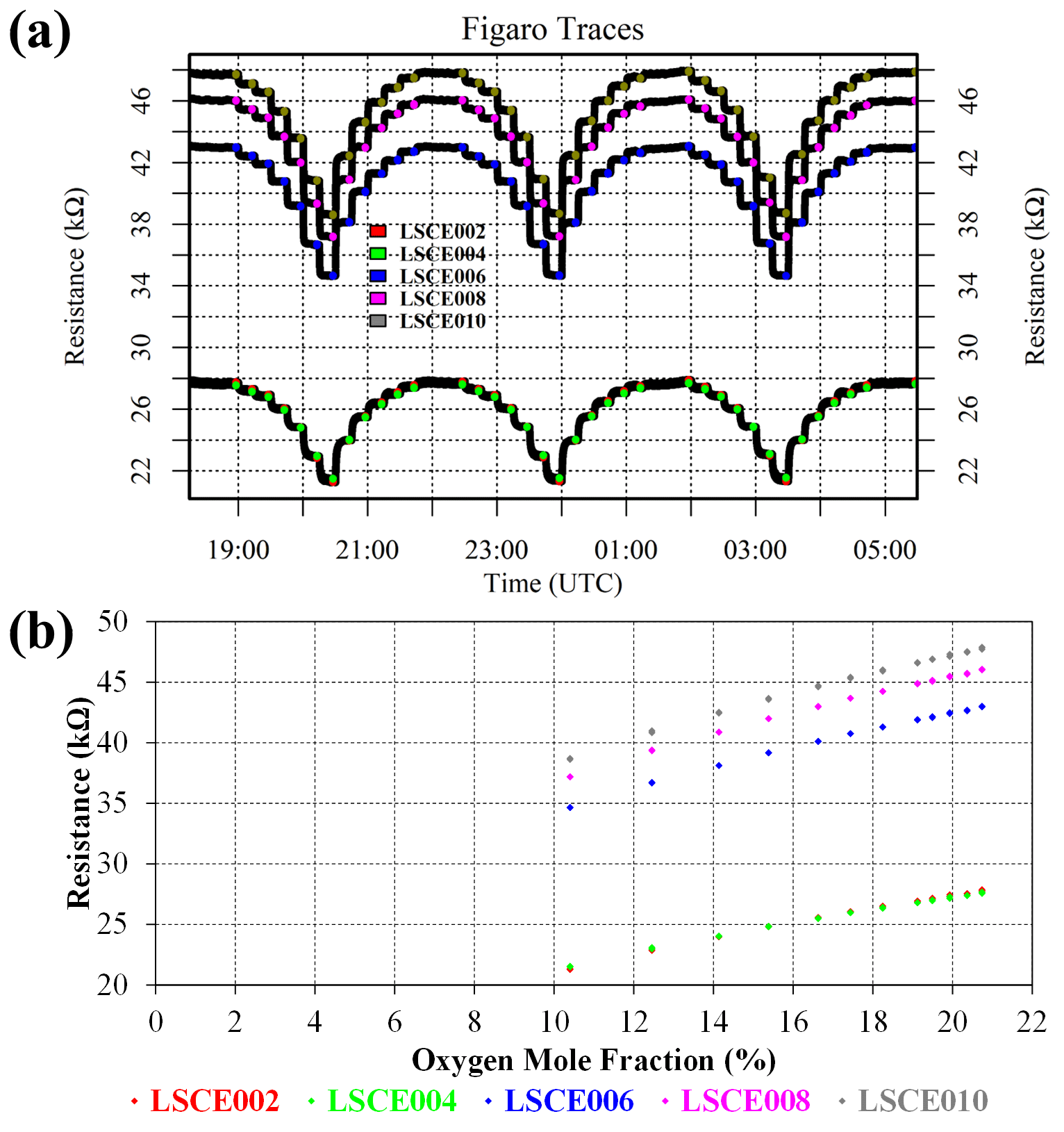
Figure 10 (a) Measured resistance for five Figaro sensors (black dots) when depleting the oxygen content of gas from a zero-air generator with nitrogen gas. Highlighted coloured dots represent periods used to derive 2 min average resistance values for each interval (see legend for corresponding sensor colours). (b) Figaro 2 min resistance averages against their corresponding oxygen mole fraction.

4 Field testing

4.1 Field deployment

Here we discuss Figaro autonomous field testing. All 10 System A loggers were deployed at the SUEZ Amailloux landfill site in the west of metropolitan France (46.7568^∘ N, 0.3547^∘ E). A landfill site served as an ideal initial field testing location, as it is a large area emission source producing CH₄ throughout the year, with occasional [CH₄] enhancements above the background of the order of 10¹ ppm. SUEZ Amailloux landfill topography gradually evolves over time as new cells are opened, filled, and then covered over with soil and geomembrane. The site features biogas collection infrastructure, in common with other European landfills (Daugela et al., 2020). The location of the 10 System A loggers is provided in Fig. 11, with an example of field installation shown in Fig. 1. The loggers were typically positioned on covered soil, away from any direct point emission sources, except for LSCE003, which was placed near a leaking vent. Three loggers were moved from an “old” to “new” location due to site evolution: LSCE001 was moved between July and November 2021, LSCE010 was moved between February and March 2022, and LSCE009 was moved on 28 April 2021.

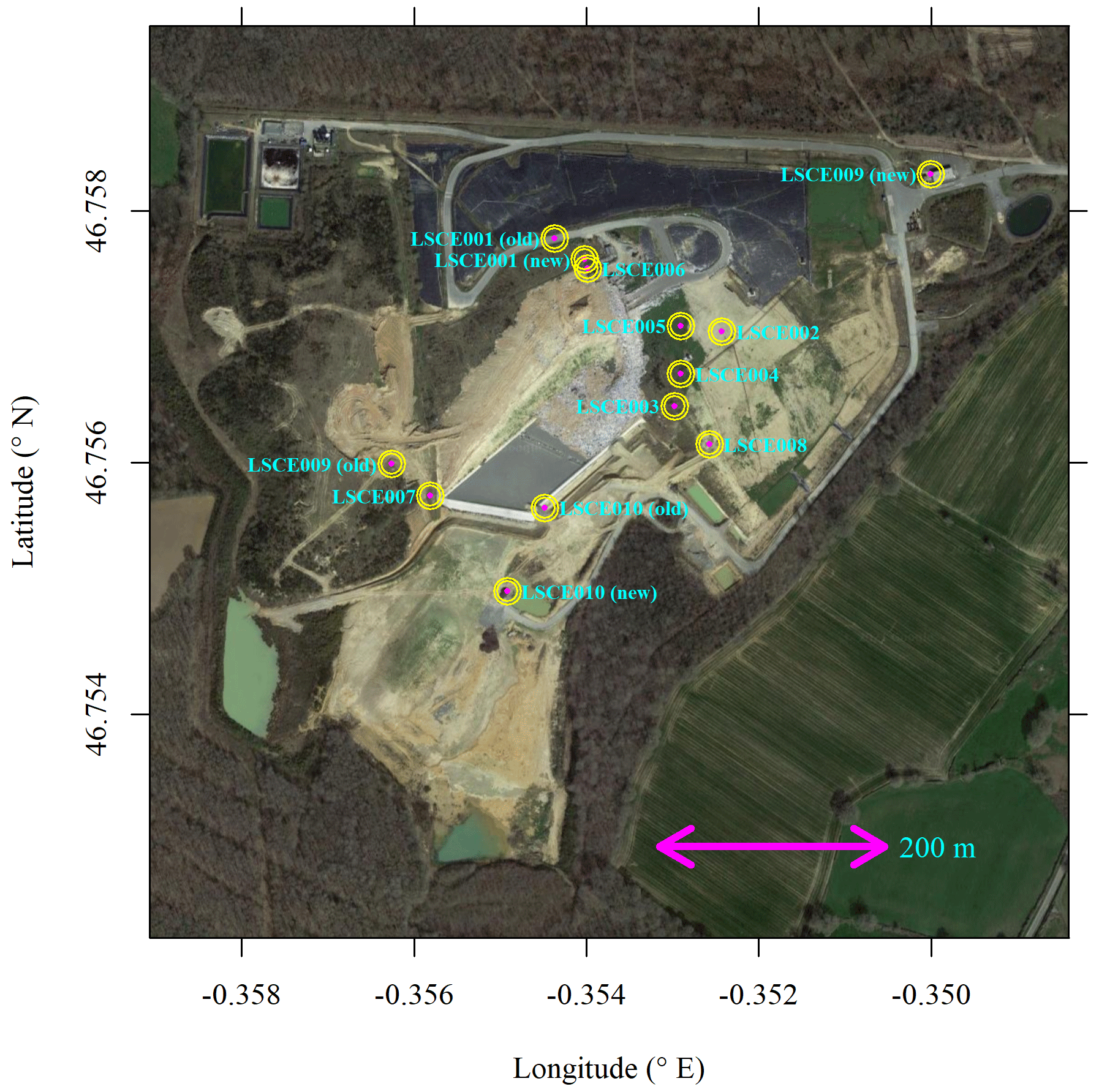
Figure 11 System A logger locations at the SUEZ Amailloux landfill site. Three sensors were moved from location “old” to location “new” (see text for details). The background image is taken from © Google Maps (imagery (2021): CNES/Airbus, Maxar Technologies).

As both [CH₄] response (Sect. 3.4) and R_2 ppm (Sect. 3.3) characterisation tests were performed on five sensors (LSCE001, LSCE003, LSCE005, LSCE007 and LSCE009), these five System A loggers will be the focus of subsequent analysis. These sensors sampled in the field between 20 March and 16 November 2021 (period 1) and then between 22 December 2021 and 27 March 2022 (period 2). Sensor testing was performed between these two sampling periods. LSCE005 stopped transmitting data on 19 October 2021. Other minor data gaps occurred due to data transmission issues.

4.2 Reference resistance modelling

For the five selected Figaro sensors, R_2 ppm was modelled for all field sampling using Eq. (4). The ratio between measured resistance and R_2 ppm may then subsequently be used to derive [CH₄], following Eq. (6). The R_2 ppm model used, as input, raw measured T_A and derived [H₂O] from the SHT85 inside each System A enclosure. [H₂O] was derived using the same procedure outlined in Sect. 3.3 where Eq. (3) was used (Murray, 1967). Modelled R_2 ppm for the five System A loggers is presented in Fig. 12 for period 1 and in Fig. 13 for period 2. Measured resistance values are also presented in Figs. 12 and 13, which show a consistently elevated measured resistance above the 5 kΩ load resistance. It may therefore be better to use a higher load resistance in future work to provide better measurement sensitivity (see Sect. 2.1). Nevertheless, 5 kΩ is plainly sufficient for this work, as small peaks and troughs are clearly detectable.

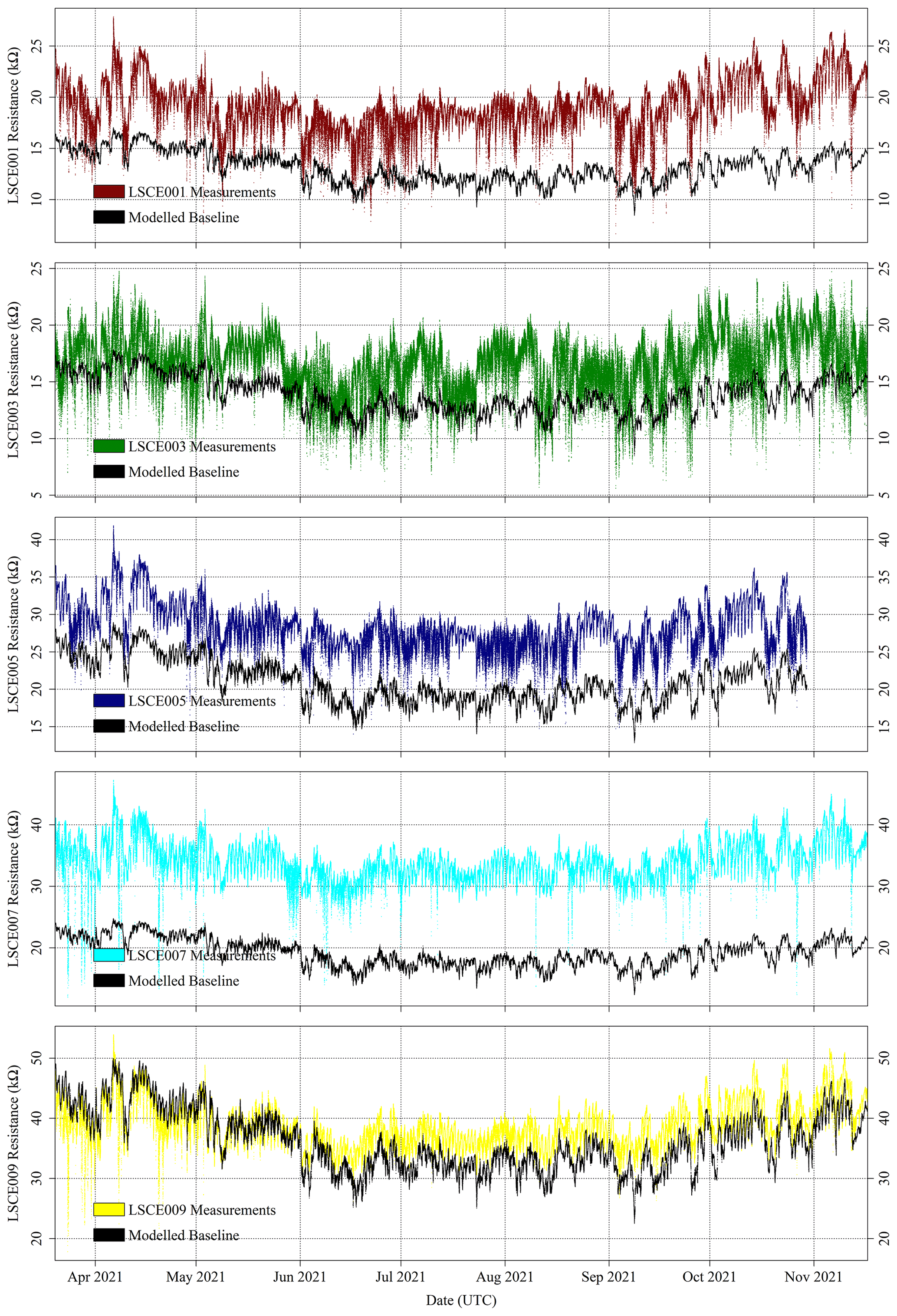
Figure 12 Measured System A Figaro resistance (coloured dots) and modelled standard 2 ppm [CH₄] reference resistance (black dots) from the SUEZ Amailloux landfill site for LSCE001, LSCE003, LSCE005, LSCE007 and LSCE009 (top to bottom) between 20 March and 17 November 2021 (period 1).

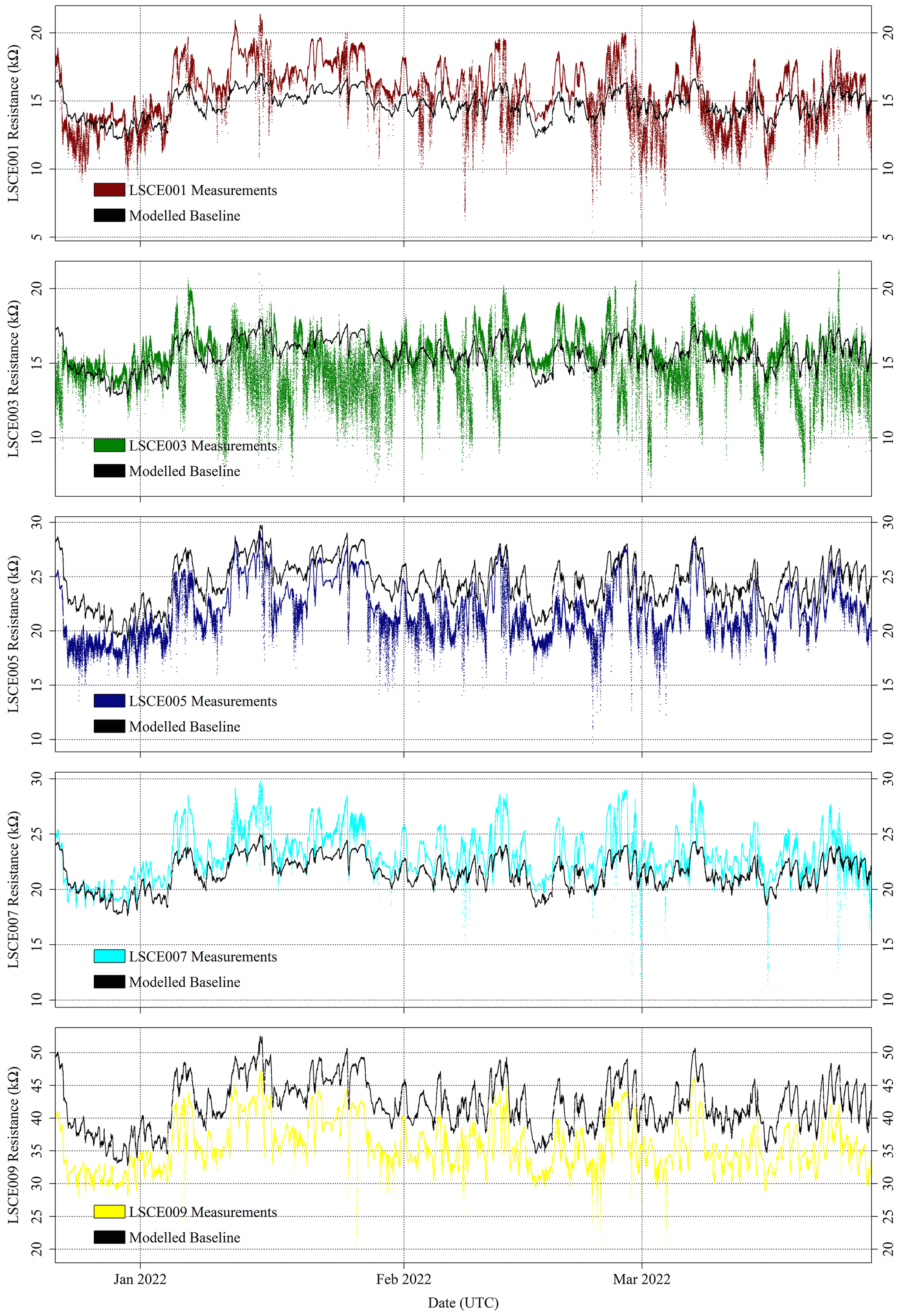
Figure 13 Measured System A Figaro resistance (coloured dots) and standard 2 ppm [CH₄] reference resistance (black dots) from the SUEZ Amailloux landfill site for LSCE001, LSCE003, LSCE005, LSCE007 and LSCE009 (top to bottom) between 22 December 2021 and 27 March 2022​​​​​​​ (period 2).

Table 5 The average ratio and P between System A measured resistance and derived standard 2 ppm [CH₄] Figaro reference resistance while sampling at the SUEZ Amailloux landfill site during period 1 and period 2. Standard deviation uncertainties for resistance ratios are given.

Figures 12 and 13 show that the Eq. (4) R_2 ppm model can replicate some features of measured resistance due to the incorporation of water and temperature effects. The Person correlation coefficient (P) between measured resistance and R_2 ppm (given in Table 5) is greater than half for all but one sensor (LSCE003) during both period 1 and period 2. Poor correlation for LSCE003 is hardly surprising, considering its placement near a leaking vent. Yet for all five sensors there is a general disparity between modelled R_2 ppm and measured resistance, which outweighs any correlation, based on average resistance ratios for both periods, provided in Table 5. For reference, a ratio between measured resistance and R_2 ppm of 1 corresponds to [CH₄] of 2 ppm (standard air). Thus, Table 5 values should be close to 1 or slightly less than 1 if generally sampling [CH₄] enhancements, as expected for LSCE003, which is near a CH₄ leak. A ratio more than 1 (i.e. when R_2 ppm is less than measured resistance) corresponds to [CH₄] below 2 ppm, which is impossible in the absence of a potent CH₄ sink.

Table 5 resistance ratio averages suggest that Eq. (4) R_2 ppm model performance is unsatisfactory for the ultimate purpose of estimating [CH₄], where an enhancement above the background of 1 ppm [CH₄] can correspond to a resistance drop of as little as 1 %. Figure 12 shows that during period 1, measured Figaro resistance was larger than R_2 ppm (a ratio greater than 1) for all five sensors most of the time, except for some overlap for LSCE009 up to June 2021. Resistance disparity was particularly stark for LSCE007, with an average period 1 resistance enhancement of +78 ± 15 % compared to R_2 ppm. Conversely, for period 2, Fig. 13 shows that resistance ratios decreased for all five sensors and were closer to 1 (see Table 5), resulting in generally better R_2 ppm agreement. However, Fig. 13 shows no period 2 improvement in capturing the nuances of daily temperature and [H₂O] variations. For LSCE005 and LSCE009, the period 2 resistance ratio was less than 1 (within the uncertainty range), which would imply consistently enhanced [CH₄] above 2 ppm that was otherwise absent during period 1 (unlikely).

The reproduction of an R_2 ppm baseline that can well-incorporate environmental variability is essential to model [CH₄] enhancements above the 2 ppm standard background level using Eq. (6). Based on model R_2 ppm and resistance measurements presented in Figs. 12 and 13, [CH₄] cannot be derived here in this way. There may be other factors causing resistance disparity; this must first be addressed before this sensor can be used to estimate parts-per-million-level [CH₄] enhancements in future, which we discuss in Sect. 5.1.

5 Discussion

5.1 Field reference resistance disparity

In this section we attempt to understand the cause of poor agreement between R_2 ppm (modelled from temperature and [H₂O]) and measured resistance, as presented in Sect. 4.2, and the reasons why 2 ppm [CH₄] reference resistance disparity was different before sensor testing (period 1) compared to after sensor testing (period 2). From Sect. 3.3, the Eq. (4) model yielded excellent R_2 ppm agreement during chamber testing (see Table 2), with an R_2 ppm RMSE below ±1 kΩ for the five tested sensors and an R² of at least 0.96. However, modelling R_2 ppm in the field was more challenging than in a controlled environment, with disparity between R_2 ppm and measured resistance up to the order of 10¹ kΩ. In addition, this resistance ratio decreased for all five sensors in period 2, though the cause of this change is not clear. As Eq. (4) model parameters were derived using the same System A field loggers, supply voltage variation is not an issue. Furthermore, high-precision voltage regulators inside System A (see Sect. 2.2) ensure that Figaro supply voltage remains the same, regardless of using a charger (in the environmental chamber) instead of a solar panel (in the field) to charge the battery. Alternatively, changes in the [CH₄] background level may have affected R_2 ppm, but this was also unlikely to be responsible, as we also conducted regular on-site and off-site sampling campaigns (not shown), during which no excessive abnormalities in general [CH₄] variability were observed. Thus, we expect emissions from the SUEZ Amailloux landfill site to remain at a relatively consistent order of magnitude throughout the year.

One possible cause of poor R_2 ppm fitting was the composition of air during environmental chamber testing. On the one hand, no [CH₄] or [CO] irregularities were observed in the chamber by the Picarro G2401 HPR. However, the results presented in Fig. 3 point to the presence of a different reducing species in air otherwise absent in clean synthetic gas (see Sect. 5.2 for further discussion). It is possible that the composition of these interfering compounds was different in the chamber compared to the landfill site, either through high-temperature chamber degassing or due to the natural ambient composition of the surrounding chamber environment. A cocktail of trace gas species (other than CH₄ and CO₂) can be emitted from landfill sites, including sulfides, ammonia, alcohols, alkanes, alkenes and aromatics, which vary by many orders of magnitude in different landfill sites (Duan et al., 2020). Yet, the pronounced resistance ratio jump from period 1 to period 2 does not support this hypothesis as the principal cause of resistance disparity. If R_2 ppm model parameters were consistently unsuitable, one would expect field resistance to consistently exceed R_2 ppm and not to erroneously decrease in period 2.

Another possibility for poor R_2 ppm agreement with measured resistance is differences in Figaro cooling dynamics in the environmental chamber compared to the field. Furthermore, van den Bossche et al. (2017) showed that the location of a temperature measurement can be highly influential concerning its application in any correction model. We therefore used the same System A logger in both applications (chamber testing and field deployment) to minimise such effects. Yet, Figaro airflow may still vary depending on conditions exterior to System A. In the field, the logging enclosures faced downwards, where lateral winds could influence upwards airflow from the downwards-facing fan due to a vacuum effect. On the other hand, boxes faced sideward in the chamber, with a large chamber fan for air circulation. These two scenarios may have cooled the Figaro sensors inside the System A enclosure differently such that the temperature gradient between the SHT85 environmental sensor and the Figaro varied, rendering the empirical Eq. (4) R_2 ppm model unusable.

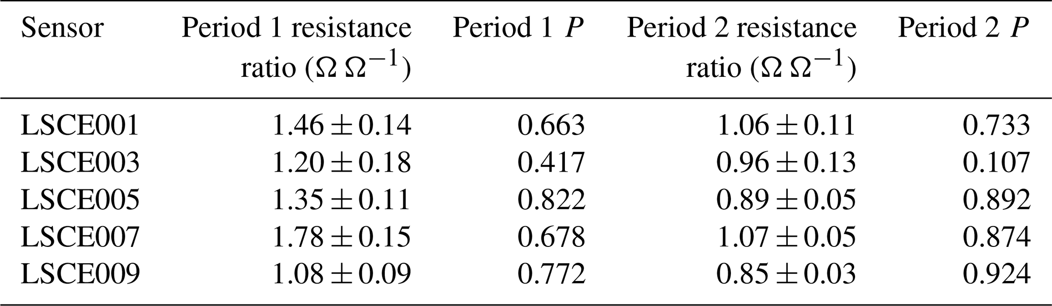
Section 4 shows that there is an unexplained jump in resistance ratio from period 1 to period 2. Yet, the above discussion suggests that the R_2 ppm model may be fundamentally flawed, either due to airflow effects or different levels of other interfering reducing gas species (see Sect. 5.2 for further discussion). Instead of resistance ratio, it may be better to analyse raw resistance measurements. Maybe, cooler and drier period 2 conditions (largely coinciding with boreal winter) erroneously exaggerated R_2 ppm. The full T_A and [H₂O] measurement range is presented in Fig. 14 for both periods as box plots for comparison, along with the measured Figaro resistance range. When actual resistance measurements are assessed, there is a large overlap between period 1 and period 2 over the full sampling range. Nevertheless, Fig. 14 shows that measured resistance was significantly lower for all five sensors in period 2 considering the interquartile range, particularly for LSCE005 and LSCE007. Yet in view of an equally significant temperature and [H₂O] period 2 decrease, it is possible that these environmental effects may account for the period 2 resistance drop if a better R_2 ppm model were used, thus improving R_2 ppm agreement with measured resistance.

Figure 14 (a) Measured Figaro resistance, (b) measured SHT85 temperature and (c) derived SHT85 water vapour mole fraction (see text for derivation details) from inside each LSCE001, LSCE003, LSCE005, LSCE007 and LSCE009 System A enclosure at the SUEZ Amailloux landfill site, shown as box plots, with outliers presented as coloured dots. Data for period 1 and period 2 are plotted separately.

A final cause of disparity between R_2 ppm and measured resistance may be spontaneous variations in the sensor itself, causing the original R_2 ppm model parameters to become invalid. However, the fact that resistance ratio decreased for all five sensors in period 2 makes this hypothesis unlikely. Instead, something may have physically altered the natural behaviour of multiple sensors during testing, such as the transfer from System A to System B or extreme [H₂O] or temperature conditions. Alternatively, high concentration exposure to certain gases can cause permanent sensor damage, which may have occurred some time between period 1 and period 2. While such effects may have been a contributory factor, the most likely cause of reference resistance disparity from actual resistance measurements (and the change in resistance ratio from period 1 to period 2) is a poor R_2 ppm model which did not suitably account for sampling conditions in the field.

5.2 Characterisation approach and future improvements

Here we discuss our general Figaro testing approach and compare our methods to other work conducted with the Figaro TGS 2611-E00, along with studies on other Figaro sensor types. In Sect. 3.2, we derived R_2 ppm using an environmental chamber. However, characterising SMO sensors using an environmental chamber calibration has proved challenging in the past. For example, Eugster et al. (2020) attempted their own chamber characterisation of the less selective (but more sensitive) Figaro TGS 2600 but yielded unsatisfactory results. They instead employed a long-term HPR field calibration (Eugster et al., 2020). Field calibration has proved popular for the TGS 2600 by using ambient HPR measurements to optimise model parameters (Eugster and Kling, 2012; Casey et al., 2019; Collier-Oxandale et al., 2019) in conditions with a similar environment and pollutant gas levels (Collier-Oxandale et al., 2018). An analogous approach can also be applied to ambient laboratory sampling by simply leaving a sensor to sample in a laboratory alongside an HPR (Rivera Martinez et al., 2021), with the aim of subsequent field deployment (Riddick et al., 2020). Yet, ambient air sensor characterisation can be problematic if various calibration models are required in different conditions, for example in different humidity (Collier-Oxandale et al., 2018) or temperature (Eugster et al., 2020) regimes.

Despite this, the Figaro TGS 2611-E00 has successfully been tested in controlled conditions in the past; for example, Cho et al. (2022) set an oven to three precise temperatures, where [CH₄] and relative humidity were externally controlled to fill a 2 dm³ test chamber. Although the application of their calibration model was tested in controlled conditions, it was not HPR field-tested (Cho et al., 2022). Furuta et al. (2022) designed a temperature-controlled TGS 2611-E00 testing chamber by placing a heated inner enclosure inside a larger freezer, where CH₄ pulses were injected into ambient air at various temperature settings. However, the sensors were not HPR field-tested, as this work was more focused on sensor characterisation (Furuta et al., 2022). As this test lacked humidity control, large [H₂O] variability occurred due to condensation and evaporation of water from the chamber walls (Furuta et al., 2022). Bastviken et al. (2020) conducted chamber testing at various temperature and humidity settings up to 3.5 % [H₂O] (humidity was indirectly controlled), where CH₄ was injected at each setting. As this calibration was designed to detect high [CH₄] in flux chambers, it was not extensively field-tested (Bastviken et al., 2020). Instead, van den Bossche et al. (2017) tested a Figaro sampling cell in a water bath for improved temperature regulation. Elsewhere, Jørgensen et al. (2020) conducted laboratory tests at three different relative humidity settings, with no temperature control, assuming constant laboratory temperature. However, they could not use this test in the field (where zero air served as a standard gas) and instead employed an HPR field calibration, assuming invariant environmental conditions (Jørgensen et al., 2020).

Yet, a key limitation of ambient air characterisation is the requirement of an expensive HPR co-located with each Figaro for a sufficiently long testing duration to derive a robust long-term model. Unless readily available, this can negate the central advantage of a cheap SMO sensor. Most of the System A loggers at the SUEZ Amailloux landfill site were isolated and distant from sources of mains power which are required by a typical CH₄ HPR. Furthermore, the site is constantly evolving, which is conducive to the deployment of low-cost sensors powered by a solar panel due to their mobility and ease of remote installation. Thus, we conducted Figaro characterisation in controlled conditions (i.e. not in the field). HPR ambient air testing of 10 System A loggers is not logistically feasible. However, it is worth noting that it may be possible to characterise R_2 ppm for multiple Figaro sensors using a single HPR by only selecting sampling during high winds, assuming the wind to sufficiently dilute any nearby CH₄ emission source (although the influence of wind on sensor cooling would need to be accounted for in such an approach). Nevertheless, a [CH₄] field characterisation cannot be achieved in this way.

Instead, our controlled chamber calibration approach required the simulation of environmental field conditions. Based on our [O₂] test (see Sect. 3.7), atmospheric pressure was dismissed as a key factor effecting the TGS 2611-E00, in agreement with other work (van den Bossche et al., 2017; Rivera Martinez et al., 2021). However, environmental chamber tests revealed a strong [H₂O] and temperature resistance response, as observed elsewhere (Bastviken et al., 2020; Rivera Martinez et al., 2021; Cho et al., 2022). Temperature may also influence electronic measurement circuitry (Ferri et al., 2009). We found [H₂O] to dominate resistance at fixed [CH₄]. We accounted for these environmental effects in our calibration approach by deriving a standard R_2 ppm, following van den Bossche et al. (2017). Whereas van den Bossche et al. (2017) derived logarithmic relationships between environmental parameters and standard resistance, we found linear correlations to be suitable.

Conversely, in many past studies testing the TGS 2600 (Eugster and Kling, 2012; Collier-Oxandale et al., 2018; Eugster et al., 2020; Riddick et al., 2020), TGS 2602 (Casey et al., 2019; Collier-Oxandale et al., 2019) and TGS 2611-E00 (Bastviken et al., 2020; Jørgensen et al., 2020; Cho et al., 2022), a fixed reference resistance has been used, in contrast to our dynamic R_2 ppm approach. Temperature and water effects have then subsequently been incorporated into models, alongside resistance ratio, to yield [CH₄] (Collier-Oxandale et al., 2018). Collier-Oxandale et al. (2019) and Casey et al. (2019) used this fixed reference approach to derive [CH₄] (as well as other gas mole fractions) by combining input from various sensors including a TGS 2600 and TGS 2602. Bastviken et al. (2020) used a combination TGS 2611-E00 environmental correction, where water and temperature were first incorporated into a dynamic reference resistance and then subsequently corrected from their resistance ratio.

Despite our best efforts, our dynamic R_2 ppm model could not replicate field Figaro resistance measurements. One cause may have been a misrepresentative temperature measurement during testing compared to field sampling (see Sect. 5.1 for specific discussion). In light of this temperature dependence, Eugster et al. (2020) proposed a TGS 2600 heat-loss model using wind speed, temperature and air heat capacities; however, this model could not predict [CH₄] any better than their original deterministic model. Elsewhere, Casey et al. (2019) found that low wind speeds adversely affected the performance of both linear and ANN [CH₄] models, whose TGS 2600 and TGS 2602 were also inside an enclosure. In light of this potential wind effect, we compared the resistance ratio with increasing minute-average wind speed for LSCE007, as measured simultaneously by the LSCE007 System A anemometer (Fig. S5 in the Supplement), where wind direction was between 180 and 270^∘ (i.e. away from the active landfill). This test showed that there is no correlation between wind speed and resistance ratio, which therefore suggests that our R_2 ppm model is not fundamentally influenced by wind speed.

All types of Figaro TGS sensors are clearly affected by water (Furuta et al., 2022). Yet, when correcting for water effects, some researchers have used relative humidity (Eugster and Kling, 2012; van den Bossche et al., 2017; Jørgensen et al., 2020; Cho et al., 2022), some have used either [H₂O] or absolute humidity (Collier-Oxandale et al., 2018; Casey et al., 2019; Collier-Oxandale et al., 2019; Eugster et al., 2020; Rivera Martinez et al., 2021; Furuta et al., 2022; Rivera Martinez et al., 2023), and some have mixed both in model combinations (Bastviken et al., 2020). As these SMO sensors respond to absolute water content, we chose [H₂O] in our R_2 ppm model, representing the fraction of water molecules in air. Absolute humidity is a mass fraction, similar to [H₂O]. On the other hand, relative humidity represents the proximity to water saturation (dew point) as a function of temperature. Thus, [H₂O] or absolute humidity typically results in superior model fitting (Bastviken et al., 2020).

Figaro sensors in general require a sufficient warm-up time before testing (Honeycutt et al., 2019; Glöckler et al., 2020; Cho et al., 2022; Furuta et al., 2022). They may also slowly age over time (Eugster et al., 2020; Riddick et al., 2020), resulting in reduced sensitivity (Eugster and Kling, 2012; Collier-Oxandale et al., 2018). Collier-Oxandale et al. (2019) resolved ageing effects by including time as a reference resistance parameter. In principle, ageing can easily be corrected by fitting between calibrations performed at two time points (Eugster and Kling, 2012). While Riddick et al. (2020) recommend bimonthly calibrations to account for time, ageing is unlikely to be an issue when targeting large (part-per-million-level) [CH₄] enhancements (Rivera Martinez et al., 2023).

During testing, we characterised each Figaro individually. Previous work has shown that despite using the same Figaro type, individual sensors behave differently (Rivera Martinez et al., 2021, 2023) due to variability in sensor surface characteristics (Bastviken et al., 2020; Riddick et al., 2020; Sieczko et al., 2020). Our results plainly show that R_2 ppm (see Table 2) and CH₄ Figaro responses (see Table 4) vary for each sensor. However, some sensors were more similar (for example LSCE001 and LSCE003) than others (LSCE009), possibly due to batch production with similar surface characteristics; sensors from the same production batch exhibit a similar CH₄ response (Furuta et al., 2022). The sensors tested in Sect. 3.4 come from various sources so they were most probably produced from at least two different batches. In the past, Cho et al. (2022) applied a single calibration model to 19 different TGS-2611-E00 sensors, but each sensor was assigned a unique fixed reference resistance. While this was crudely laboratory-tested, with an average 8 ppm [CH₄] deviation (sampling up to 190 ppm), it is not clear if this approach was valid in the field (Cho et al., 2022). Elsewhere, Collier-Oxandale et al. (2018) tested a universal TGS 2600 calibration model, which while promising, could not compete with a sensor-specific model, supporting our approach.

Although our R_2 ppm model requires improvement, [CH₄] response was characterised very well up to 1000 ppm in controlled conditions, with a resistance ratio RMSE of no more than ±1 % Ω Ω⁻¹ for the five tested sensors and an R² of at least 0.997. Our Eq. (6) [CH₄] model is similar to the simple manufacturer-proposed power law (Eugster and Kling, 2012). However, as we used resistance ratio instead of raw resistance, we included a unity term. This satisfies the requirement that the resistance ratio is equal to 1 in standard gas (i.e. when [CH₄] is 2 ppm). Furthermore, Eq. (5) allows other sensitive gases to be multiplicatively included.

Our Fig. 8 resistance decay curve is similar to the TGS 2611-C00 relationship overserved by Glöckler et al. (2020) up to 9000 ppm [CH₄], although they did not derive a model fit. Honeycutt et al. (2019) proposed a Langmuirian fit in dry conditions up to 1000 ppm [CH₄] for various Figaro types. Instead of using a reference resistance, Furuta et al. (2022) devised a simple [CH₄] model for various Figaro types up to 10 ppm based solely on [H₂O] and sensor resistance, resulting in ±1 ppm [CH₄] RMSE for three different tested TGS 2611-E00 units. Elsewhere, Rivera Martinez et al. (2021) found a clear resistance decline up to 9 ppm [CH₄], but Figaro TGS 2611-E00 resistance changes were less pronounced than for the TGS 2600 and TGS 2611-C00. The van den Bossche et al. (2017) study yielded a linear TGS 2611-E00 [CH₄] calibration by sampling six [CH₄] levels up to 9 ppm in fixed environmental conditions. Although TGS 2611-E00 resistance appears linear over a small [CH₄] range, non-linearity increases at higher [CH₄] (Honeycutt et al., 2019; Bastviken et al., 2020). Cho et al. (2022) derived a resistance power law up to 10 000 ppm [CH₄] at various temperature settings. Jørgensen et al. (2020) also observed a resistance ratio power fit up to 100 ppm [CH₄]. A similar fit was observed at three different relative humidity settings; however, this model did not include a unity term as in Eq. (5) (Jørgensen et al., 2020), meaning that resistance tends to infinity at standard [CH₄], rather than a limiting reference resistance. A simple power law also limits the model to a single gas.

As Jørgensen et al. (2020) and Cho et al. (2022) targeted emissions where CH₄ is the primary reducing gas, their calibration models only included CH₄. We followed a similar approach for our landfill emission source by simplifying Eq. (5) to Eq. (6). Alternatively, the TGS 2611-C00 or even the TGS 2600 may be used where only small interfering CO enhancements are expected, as the lack of a CO filter amplifies CH₄ sensitivity (Eugster et al., 2020). In addition, Rivera Martinez et al. (2023) showed that the TGS 2611-C00 may be less noisy, making it easier to model [CH₄] enhancements above the background than the TGS 2611-E00. This improved TGS 2611-C00 sensitivity may augment an environmental R_2 ppm fit. In any case, our Eq. (5) model allows other gases to be included in future work if necessary. This may allow the TGS 2611-E00 to be deployed in industrial locations with high CO emissions. However, before considering such an approach, improvements in R_2 ppm characterisation are first required. The small resistance decrease (between 1.4 % and 2.0 % for the five tested sensors; see Table 4) in response to a 1 ppm [CH₄] enhancement above the background emphasises the importance of accurately modelling R_2 ppm.

Reference gas testing (Sect. 3.2) revealed that synthetic air and ambient air (from our laboratory), containing the same 2 ppm [CH₄], resulted in a different Figaro resistance response. A similar effect may have also contributed to disparity between landfill Figaro measurements and R_2 ppm due to a different air composition in the environmental chamber compared to the field. A precise gas analysis may identify Figaro-sensitive species in different gas sources, including ambient air at the landfill site (Duan et al., 2020), using techniques such as gas chromatography, Fourier-transform IR spectroscopy or proton-transfer-reaction mass spectrometry, which is particularly suited to detect volatile organic compounds. However, in reality, this would be arduous as it is not clear which interfering gases to look for, especially at a landfill site (Duan et al., 2020). CH₄ is the most abundant reducing gas in natural ambient air followed by CO, which were both measured by the Picarro G2401 HPR throughout testing in the environmental chamber and during the laboratory sensitivity tests. Although other alkanes (for example, ethane, propane and butane) are reducing gases with chemical properties similar to CH₄, they are present in very low quantities in ambient air. Furthermore, manufacturer testing with isobutane up to 10 000 ppm revealed negligible Figaro resistance response (Figaro Engineering Inc., 2021), though straight-chain alkanes may behave differently. Similarly, alcohols may interfere with SMO sensors, but manufacturer testing up to 10 000 ppm of ethanol also showed negligible Figaro response (Figaro Engineering Inc., 2021). Hydrogen is the only other reducing gas known to affect the Figaro TGS 2611-E00 (Figaro Engineering Inc., 2021). Maybe different alcohols and alkanes (or some other volatile organic compounds, not discussed here) could play a role, but targeting a specific reducing species, with no obvious candidate, remains a challenge. Unfortunately, it is difficult to look to other SMO prototype sensors to help identify Figaro-sensitive interfering compounds, as each SMO sensor is unique in its composition and behaviour. Therefore, we recommend a robust analysis of Figaro TGS 2611-E00 gas sensitivities in future work to help identify potential interfering gas species in ambient air. In this work, for simplicity, we used ambient air as a standard gas rather than clean synthetic gas or zero air when characterising R_2 ppm. However, this assumes that the air composition during testing was similar to ambient air in the field. A thorough gas analysis may help to confirm this assumption. Alternatively, deploying a field logger containing a suite of low-cost SMO sensors with sensitivities to different gases (including and excluding CH₄) may help to shed some light on the nature of interfering reducing compounds (Casey et al., 2019; Collier-Oxandale et al., 2019). Such a future test may offer valuable insight into various Figaro sensitivities over a prolonged sampling period.

Another potential cause of resistance disparity between the R_2 ppm model and landfill Figaro sampling was the wind dynamics around the System A enclosure, as discussed above. This may be resolved by placing the Figaro sensor in a closed cell more akin to System B. This permits a controlled sensor airflow, resulting in consistent sensor cooling effects. It also buffers temperature changes and allows temperature measurements to be more repeatable in the laboratory compared to the field. This approach would also enable precise gas exposure during environmental R_2 ppm testing rather than relying on potentially contaminated air in and around an environmental chamber. Furthermore, the Figaro sensor would not move between loggers, eliminating the chance of different loggers potentially causing spurious jumps in sensor behaviour. However, a closed-cell logger requires a pump, which has substantially higher power requirements. This may push a solar panel power source to its limits, especially in the mid-latitude winter.

6 Conclusion

A total of 10 Figaro TGS 2611-E00 sensors were deployed at a landfill site in France, 5 of which were tested to characterise environmental and methane gas response. The ultimate objective was to derive methane mole fraction from sensor resistance. Our characterisation approach first separated environmental effects by incorporating them into a standard reference resistance. This enabled the independent characterisation of sensor response to individual reducing gas species.

Before characterising an environmental baseline resistance (independent of gas composition), we found that the choice of standard reference gas has a significant effect on Figaro resistance, despite each gas sample containing the same 2 ppm methane mole fraction: Figaro resistance was much lower in natural ambient air compared to both synthetic air and a high-concentration methane source diluted with zero air (to target 2 ppm methane mole fraction). We therefore used ambient laboratory air as our testing gas standard, which naturally contains 2 ppm of methane. Sensor response to temperature and water vapour mole fraction was then characterised in the field logging enclosure, which was placed inside a large environmental chamber. A four-parameter model was then used to yield reference resistance from water vapour mole fraction and temperature; the former had the largest influence on resistance.

This model was then applied to field sampling, where methane mole fraction was mostly at background levels (2 ppm). In spite of the capability of the environmental chamber model fit to derive reference resistance under controlled conditions at 2 ppm methane mole fraction, reference resistance could not be replicated in field conditions for a variety of potential reasons. There may have been differences in airflow around the logger in the field compared to the environmental chamber, the air composition may have been different during chamber testing, or there may have been spontaneous sensor variability during transfer between various loggers and in different environments.

Nevertheless, our independent methane gas enhancement characterisation model provided an excellent fit in controlled conditions. This was achieved by taking the ratio between measured resistance and a reference (background methane) resistance when sampling up to 1000 ppm methane mole fraction in incremental steps. We conceived an adapted power fit between methane mole fraction and this resistance ratio, with a coefficient of determination of at least 0.999. When this model was inverted to make methane mole fraction the subject, we derived a root mean squared error of less than ±1 ppm when limited to below 28 ppm. We also showed that the effect of carbon monoxide is minimal during similar sensitivity tests.

We propose that future TGS 2611-E00 work should be conducted with great care to ensure that environmental effects are well-characterised and that an appropriate choice of standard gas is used to mirror field sampling conditions. With improvements in a reference (standard gas) resistance characterisation, it is evident that the Figaro TGS 2611-E00 sensor has great potential in detecting methane mole fraction with parts-per-million-level precision. A closed sampling cell with a pump may help to achieve this goal, although power requirements will have to be taken into consideration.

Appendix A: Influence of supply voltage

The influence of power supply voltage on both resistance and CH₄ sensitivity was characterised by testing a Figaro sensor (LSCE009) in System B in our air-conditioned laboratory. V_s was adjusted from the high-precision power supply unit (T3PS23203P, Teledyne LeCroy Inc.) in four tests: test 1 was at a V_s of 5.00 V, test 2 was at a V_s of 5.10 V, test 3 was at a V_s of 5.00 V and test 4 was at a V_s of 5.10 V. During each test, gas from the zero-air generator was first sampled for at least 1 h. Then an ambient target gas cylinder filled with outside air (1.6 ppm [CO], 2.2 ppm [CH₄] and 434 ppm [CO₂]) was sampled in four 15 min intervals. Each ambient target gas interval was followed by 15 min of sampling zero-air generator gas. A fixed 8 ^∘C dew point was used throughout testing. Gas at this dew point was sampled from at least 24 h in advance of test 1.

Figaro resistance results for the four tests are presented in Fig. A1. For each test, a 2 min average was taken at the end each 15 min ambient target gas sampling interval, except the first (see Fig. A1). A 0 ppm reference resistance baseline was then derived by fitting a second-order polynomial to the final 2 min of each 15 min zero-air sampling period. [H₂O] was on average 0.975 ± 0.001 % during these 2 min zero-air periods for all four tests, according to the Picarro G2401, and System B temperature was on average 27.9 ± 0.1 ^∘C, according to the SHT85 sensor inside the sampling cell.

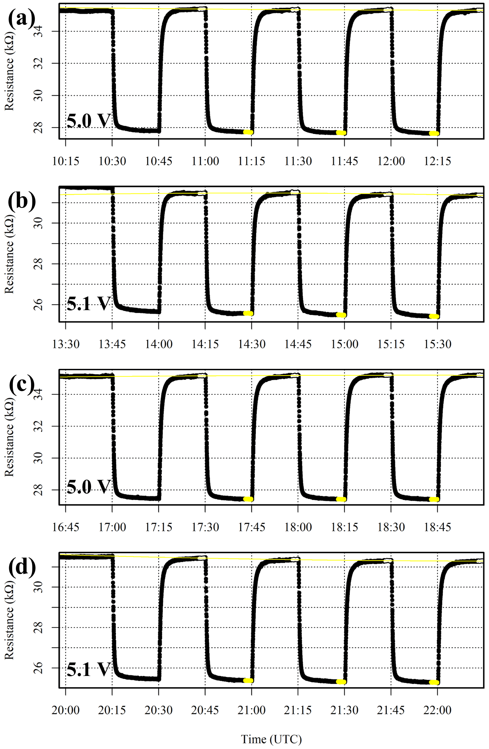
Figure A1 Measured LSCE009 resistance (black dots) when varying between zero air and ambient target gas for (a) test 1 at 5.00 V, (b) test 2 at 5.10 V, (c) test 3 at 5.00 V and (d) test 4 at 5.10 V supply voltage. Highlighted yellow dots show 2 min periods used to derive an average resistance value for three ambient target gas sampling periods. White-highlighted dots indicate periods used to derive zero-air baseline resistances, and yellow lines show respective polynomial baseline fits.

The ratio between each 2 min average ambient target gas resistance and its corresponding modelled zero-air reference resistance was acquired. Each of the four tests yielded three resistance ratios (see Table A1). In addition, for each test, all zero-air and ambient target gas 2 min average resistance measurements were combined and averaged in Table A1. These results show that Figaro resistance is consistently lower at higher V_s; for example, zero-air resistance at 5.00 V is 35 kΩ, whereas at 5.10 V it drops to 31 kΩ. This test also shows that Figaro sensitivity is consistently lower at a higher voltage owing to a lower resistance ratio. At 5.00 V, the resistance decreases by 22 % when transitioning from zero air to ambient target gas, whereas at 5.10 V, there is a smaller 19 % resistance decrease.

This resistance and sensitivity decrease at 5.10 V emphasises the importance of maintaining a fixed and reliable 5 V V_s to maintain consistency between sensor testing and field application. This effect is possibly due to a higher heater temperature at higher V_s, resulting in lower resistance, as proposed in Eq. (4). Similarly, van den Bossche et al. (2017) found that a 10 mV change in heater voltage resulted in a roughly 1 ppm error in their [CH₄] estimate at constant ambient temperature. However, this does not explain reduced Figaro sensitivity. This sensitivity effect may be caused by a change in the density of electrons within the SMO conduction band under an elevated potential difference.

Table A1 Average zero-air and ambient target gas resistances during 2 min averaging periods for four tests at two different supply voltage settings. The resistance ratio for each 2 min ambient target gas average is given, compared to a zero-air baseline reference resistance.

Appendix B: Water response delay

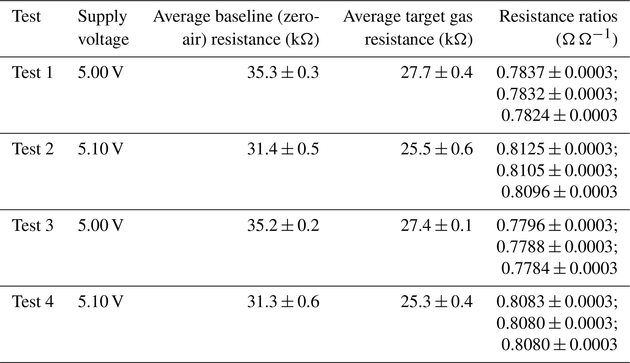
Figaro sensors exhibit a delayed response to [H₂O] changes. Figure B1 shows an example of [H₂O] decrease, while a Figaro sensor (LSCE010) continuously sampled gas from the zero-air generator in System B. The dew-point setting was abruptly reduced from 20 to 8 ^∘C, resulting in a 1 % [H₂O] drop. Sensor resistance appeared to overshoot in response to this [H₂O] change and slowly decayed back to a stable level over many hours. [H₂O] was (1.116 ± 0.002) % between 07:30 and 14:30 UTC, according to the Picarro G2401, while System B temperature was 30.2 ± 0.2 ^∘C, according to the SHT85 inside the cell, with a small 0.07 ^∘C h⁻¹ increase (when applying a linear fit). This negligible temperature change suggests that the observed resistance decay is predominantly an artefact of the water transition. The cause of this effect is not fully understood. It may be related to water desorption dynamics on the surfaces between grain boundaries. Water desorption may not be homogenous throughout the sensor, causing a prolonged delay in reaching a resistance equilibrium. Whereas Rivera Martinez et al. (2021) allowed 35 min and van den Bossche et al. (2017) allowed 70 min for [H₂O] stabilisation, our test shows that many hours of sampling at fixed [H₂O] are needed for sufficient water stabilisation; 1 full day of constant Figaro exposure is recommended.

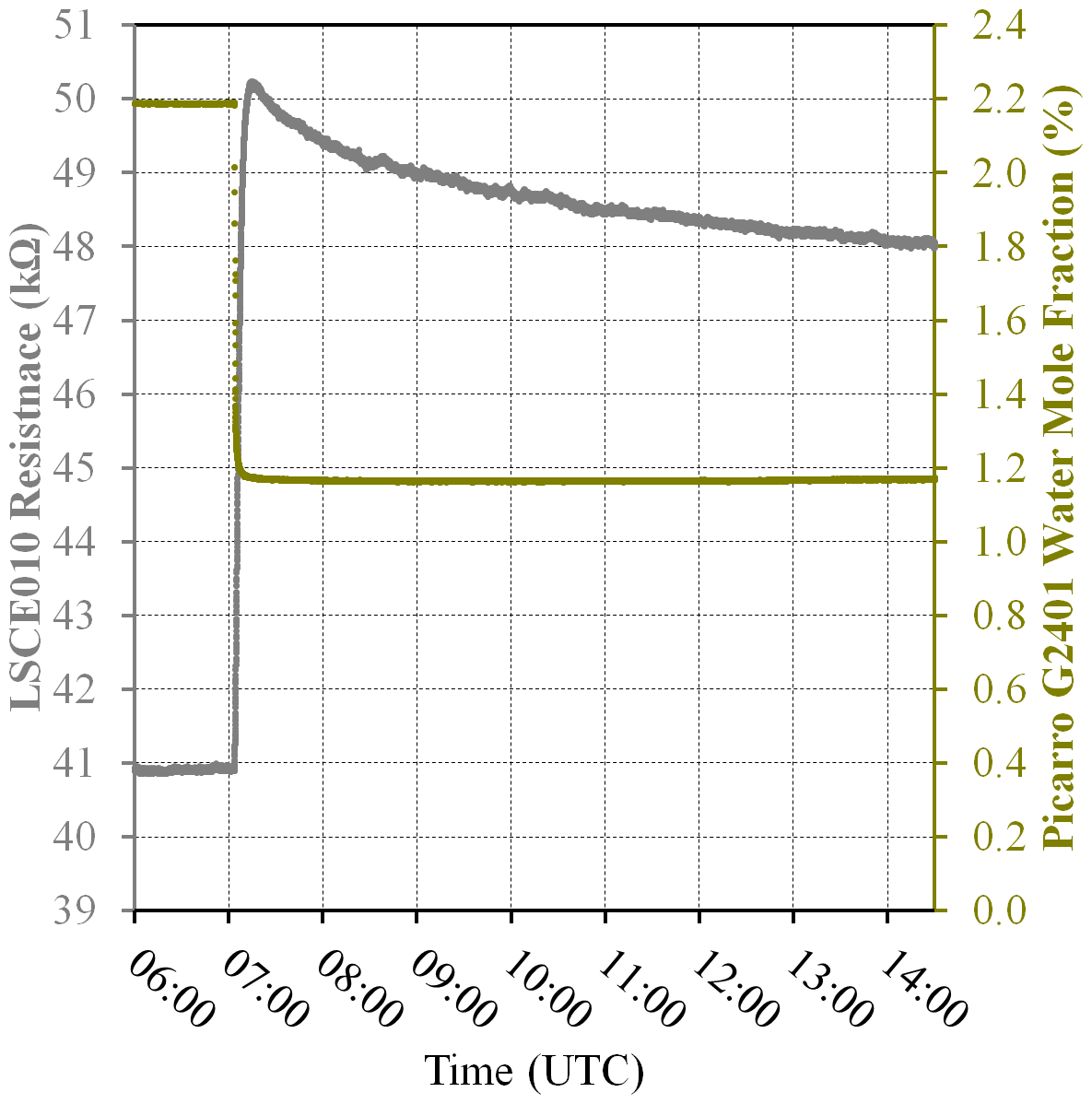
Figure B1 Figaro LSCE010 measured resistance (grey points; left-hand axis) in response to a water vapour mole fraction drop, as measured by the Picarro G2401 (dark yellow points; right-hand axis), while sampling zero-air generator gas inside System B.