Controlled-release testing of the static chamber methodology for direct measurements of methane emissions

Direct measurements of methane emissions at the component level provide the level of detail necessary for the development of actionable mitigation strategies. As such, there is a need to understand the magnitude of component-level methane emission sources and to test methane quantification methods that can capture methane emissions at the component level used in national inventories. The static chamber method is a direct measurement technique that has been applied to measure large and complex methane sources, such as oil and gas infrastructure. In this work, we compile methane emission factors from the Intergovernmental Panel on Climate Change (IPCC) Emission Factor Database in order to understand the magnitude of component-level methane flow rates, review the tested flow rates and measurement techniques from 40 controlled-release experiments, and perform 64 controlled-release tests of the static chamber methodology with mass flow rates of 1.02, 10.2, 102, and 512 g h⁻¹ of methane. We vary the leak properties, chamber shapes, chamber sizes, and use of fans to evaluate how these factors affect the accuracy of the static chamber method. We find that 99 % of the component-level methane emission rates from the IPCC Emission Factor Database are below 100 g h⁻¹ and that 77 % of the previously available controlled-release experiments did not test for methane mass flow rates below 100 g h⁻¹. We also find that the static chamber method quantified methane flow rates with an overall accuracy of $+\mathrm{14}/-\mathrm{14}$ % and that optimal chamber configurations (i.e., chamber shape, volume, and use of fans) can improve accuracy to below ±5 %. We note that smaller chambers (≤20 L) performed better than larger-volume chambers (≥20 L), regardless of the chamber shape or use of fans. However, we found that the use of fans can substantially increase the accuracy of larger chambers, especially at higher methane mass flow rates (≥100 g h⁻¹). Overall, our findings can be used to engineer static chamber systems for future direct measurement campaigns targeting a wide range of sources, including landfills, sewerage utility holes, and oil and natural gas infrastructure.

1 Introduction

Methane is a potent greenhouse gas, and international initiatives such as the Global Methane Pledge (EC, 2021) have motivated national commitments towards reducing emissions of methane from a variety of sectors ranging from waste and energy to agriculture. In order to materialize methane reductions through actionable mitigation strategies, accurate methane inventories that quantify methane from different sectors and sources are needed. Methane emission sources can be broadly classified as either site- or component-level emissions, where site-level emissions are the sum of multiple emitting components. There are also additional classifications such as facility, regional, continental, and global level (NACEM, 2018) that encompass each preceding classification within a larger agglomeration of methane emission sources. Understanding methane emissions at the component level (i.e., the smallest tier of methane emission sources) is particularly important for developing actionable methane reduction strategies, as these data can be used to directly analyze the cost benefits of mitigation options, thereby allowing policymakers and project developers to make informed decisions (Kang et al., 2019; IEA, 2021). Thus, it is important that we test and develop methane quantification methods that are capable of measuring methane emissions accurately at the component level.

To select the optimal methane measurement methods, there is a need to understand the expected magnitude of methane emission rates from different component-level sources. Some data sources, such as the Intergovernmental Panel on Climate Change (IPCC) Emission Factor Database (IPCC EFDB, 2022), have compiled emission factors for different greenhouse gas sources around the world. However, some emission factors within this database are provided at the site level, whereas others are provided in alternative forms to methane emission rates (e.g., the mass of methane emitted per ton of waste), making it difficult to determine the magnitude of expected component-level emission rates. As such, our goal is to determine the approximate magnitude of methane emission rates at the component level so that we can conduct tests at appropriate methane flow rates.

There are multiple methods that are used to quantify methane emissions; we classify these methods as either indirect or direct methods. Indirect methane quantification methods are based on measurements made away from the source of emissions, and they can often be conducted without site access. These methods include mobile surveys, stationary tower measurements (e.g., eddy covariance towers), aerial-based surveys, and satellite measurements (Cusworth et al., 2022; Edie et al., 2020; Robertson et al., 2017; Kumar et al., 2022; Riddick et al., 2022; Ravikumar et al., 2017; Ayasse et al., 2019; Cooper et al., 2022; Varon et al., 2018; de Foy et al., 2023; Chopra, 2020; MacKay et al., 2021; Tyner and Johnson, 2021). Direct methane quantification methods are based on quantifying methane emissions directly at the emission source and generally require site access. The most common direct measurement methods include optical gas imaging cameras, Hi Flow samplers, and chamber-based methodologies.

Methane sources can be classified as component-, site-, facility-, regional-, or global-level sources in order of increasing spatial scale (NACEM, 2018). As an example, a valve on an oil and gas well would constitute a component-level source, whereas all oil and gas wells in the Appalachian Basin would comprise a regional-level methane source. The advantages of methane inventories created from component-level measurements are their high resolution and easy comparisons to regional inventories, which are predominantly made using component-level data (EPA, 2021; ECCC, 2021), where specific discrepancies can be identified (Rutherford et al., 2021). Indirect measurements can be used to measure methane emissions at site, facility, or regional levels. On the other hand, direct measurement methods are labor-intensive and can omit methane sources when scaling up measurements to facility, regional, or global levels, but they can quantify and attribute methane emissions at the component level. In terms of testing methane measurement methods for accuracy, the majority of the published literature has focused on indirect methods (e.g., Robertson et al., 2017; Edie et al., 2020; Sherwin et al., 2021; Aubrey et al., 2013), whereas few studies have tested and quantified the accuracy of direct measurement methods (Riddick et al., 2022; Pihlatie et al., 2013; Christiansen et al., 2011).

Among the direct measurement methods, optical gas imaging cameras and Hi Flow samplers both have limits of detection of roughly 20 g h⁻¹ (Ravikumar et al., 2017; Fox et al., 2019). However, the stated uncertainties of optical gas imaging cameras in Fox et al. (2019) of 3 %–15 % are noted as being complex and likely much higher, and there have been several studies that have highlighted measurement errors attributed to the Hi Flow sampler (Connolly et al., 2019; Howard et al., 2015). As an alternative, the static chamber methodology is a well-established, direct methane measurement method (Riddick et al., 2022; Pihlatie et al., 2013) that is traditionally used in the measurement of methane and other trace gas emissions from soils (Conen and Smith, 1998; Raich et al., 1990; Smith and Cresser, 2003). In recent years, the static chamber method has been applied in a wide range of settings, such as the quantification of methane emissions from oil and gas wells (Alvarez et al., 2018; Lebel et al., 2020; Williams et al., 2020; Kang et al., 2014; El Hachem and Kang, 2022; Townsend-Small et al., 2016; Townsend-Small and Hoschouer, 2021; Saint-Vincent et al., 2020; Riddick et al., 2019), sewage utility holes (Fries et al., 2018; Williams et al., 2022), landfill vents and observation wells (Williams et al., 2022), and natural gas (NG) distribution infrastructure (Williams et al., 2022; Lamb et al., 2016, 2015). All of these sources vary in terms of their leakage properties and structural complexity with respect to the installation of chambers over leaking components. However, few studies have quantified the measurement accuracy of the static chamber method, and even fewer (Riddick et al., 2022; Lebel et al., 2020) have tested the static chamber method under conditions that mimic the wide range of settings in which they are now being used.

Different methane sources can emit methane at the same mass flow rates, albeit at different volumetric flow rates depending on the methane concentration of the source. For example, biogas produced from landfills (∼50 % methane) will differ with respect to its source methane concentration compared with NG from a distribution pipeline (∼90 % methane). To our knowledge, there have been no studies that have tested the effects of a varying volumetric flow rate of methane as a factor to be considered in measurement accuracy for any methane measurement method. In terms of the structural complexity of these sites, several studies have employed large chambers with suboptimal shapes to accommodate more complex sites. For example, a study by Lebel et al. (2020) in California targeting oil and gas wells used three static chambers that differed with respect to size (i.e., from 33.8 to 32 659 L) and shape (i.e., cylindrical and rectangular configurations). A key assumption in the static chamber method is that the air and gas within the chamber are well mixed (Kang et al., 2014). If the emission rate is low and the chamber is large, it may be challenging to ensure that the gases in the chamber are well mixed. Some chamber shapes, such as rectangular shapes, have been shown to have “dead zones” where gases are not well mixed, thereby lowering the effective volume of the chamber (Christiansen et al., 2011).

In this work, we (1) compile component-level methane emission factors and categorize them by source category; (2) investigate prior controlled-release testing of direct and indirect methane measurement methods to identify gaps in testing; (3) test the impacts of physical factors such as the chamber shape, size, and use of fans on the accuracy of methane flow rate estimates; and (4) test the effects of leak properties (i.e., mass flow rates, volumetric flow rates, and the concentration of methane in the leak) on the accuracy of chamber measurements. Our results highlight the applicability of the static chamber technique in direct measurements of methane emissions and provide the detail necessary to inform future measurement campaigns.

2 Methodology

We compiled a dataset of methane emission factors from the IPCC Emission Factor Database (IPCC EFDB, 2022) and categorized them into three source categories: agriculture, forestry, and other land use (AFOLU); energy; and waste. We removed all emission factors that were not related to direct mass flow rates of methane at the component level. We also removed all emission factors presented as methane flux rates (i.e., the mass of methane emitted over a given area) and, where possible, converted all remaining methane emission factors to component-level methane mass flow rates presented in grams of methane emitted per hour, based on the assumptions outlined in Table S1 in the Supplement.

We performed a literature review of 40 controlled-release experiments of methane using both indirect and direct methods to evaluate the range of methane flow rates tested and the methods used. The criteria for the literature review included all studies where methane was released at known mass flow rates (of methane) from aboveground points and excluded studies related to methane released in the subsurface, laboratory experiments of methane plume transport through porous media, and studies in which the tested mass flow rates of methane were not reported. We also exclude studies in which methane quantification methods were tested on in situ methane sources for validation. We categorized the studies based on the tested measurement platforms, which we grouped into the following eight categories: satellite (indirect method), crewed aerial vehicle (indirect method), uncrewed aerial vehicle (indirect method), stationary tower (indirect method), mobile survey (indirect method), Hi Flow sampler (direct method), camera-based measurements (direct method), chamber measurements (direct method), and/or a combination of all of the above.

We performed controlled releases of methane for the static chamber method outdoors on the McGill University campus in Montréal, Canada, on 2, 8, and 10 June 2021. The weather on these days was sunny with sparse clouds, an average temperature of 25 %C, and wind speeds ranging from 5 to 15 km h⁻¹ (World Meteorological Station ID: 71612). We designed the controlled-release experiments to test a combination of six different factors: mass flow rate, volumetric flow rate, methane percentage of leaking gas, chamber shape (i.e., rectangular versus circular), chamber size (i.e., 14, 18, 322, and 2265 L), and the use of fans within the chamber. For the 322 and 2265 L chambers, we used four battery-powered equipment cooling fans (airflow of 40 ft³ min⁻¹ or 1.1m³ min⁻¹) installed at the top of the chamber framework and oriented at 45^∘ angles downward into the chamber, whereas we used one fan for the smaller chambers. The tested chamber shapes were a 2265 L rectangular chamber, a 322 L cylindrical chamber, an 18 L cylindrical chamber, and a 14 L rectangular chamber (Table 1). In addition, for a qualitative comparison between chamber sizes, we define the ≤20 L chambers as small and the 322 and 2265 L chambers as large. Other factors, such as the aspect ratio of the chamber, the rigidity of the chamber material, and the type of chamber material, are provided in Table 1.

Table 1 Physical descriptions of chambers used for the controlled-release experiments. Qualitative descriptions of chamber volume are indicated in parentheses in the first row.

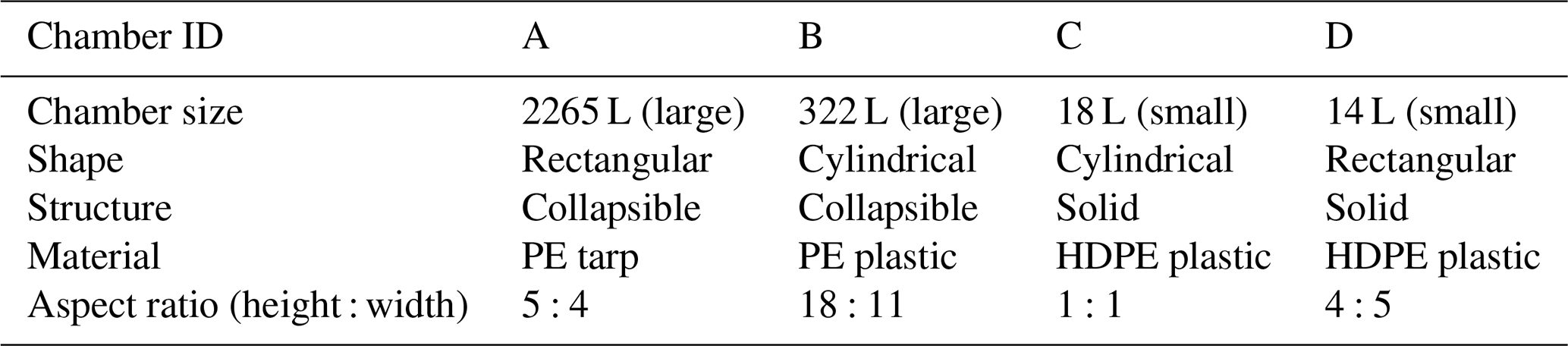
The abbreviations in the table are as follows: PE – polyethylene and HDPE – high-density polyethylene

We tested four different mass flow rates: 1.02, 10.2, 102, and 512 g h⁻¹. In order to provide a qualitative comparison between mass flow rates, we define the mass flow rates of 1.02 and 10.2 g h⁻¹ as low flow rates and the 102 and 512 g h⁻¹ releases as high flow rates. At least two different volumetric flow rates and two different methane concentrations were used for each of the mass flow rates that we tested. The volumetric flow rates ranged from 0.238 to 23.8 slpm (standard liters per minute) for a total of 10 unique leaks (Table 2). We controlled the mass flow rates of methane using two mass flow controllers (Masterflex mass flowmeter controller) with respective volumetric flow ranges of 50–0.5 and 1–0.01 slpm (error of ±0.8 % of reading and ±0.2 % of full-scale range). Both mass flow controllers were factory calibrated prior to use for these experiments. Four different methane standards, prepared by Linde Canada, were used in our study: 100 %, 50 %, 10 %, and 5 % methane (±0.5 %) – all with a gas balance of air.

Table 2 Leak properties of 10 different leaks used in controlled-release experiments, including the percentage errors associated with the mass flow controllers (MFCs). Qualitative descriptions of the leak sizes are given in parentheses in the first column.

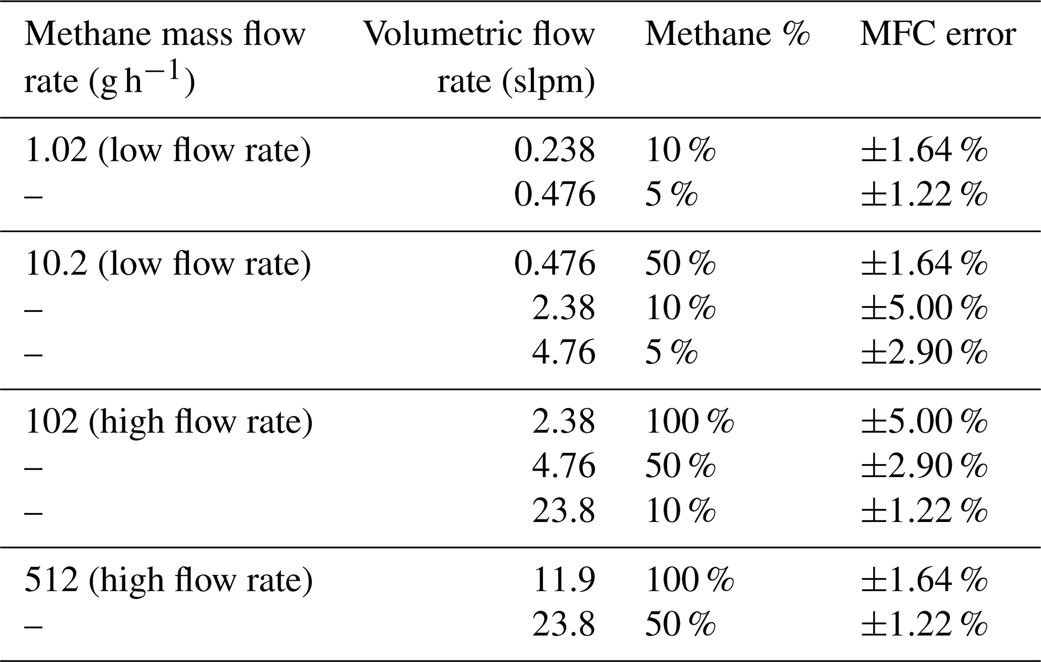
The abbreviations used in the table are as follows: slpm – standard liters per minute and MFC – mass flow controller

We performed the controlled-release tests by releasing methane through TYGON tubing connected to the chamber (Fig. 1). We oriented the tubing to the center of the chamber and secured it to the ground with tape to orient the flow upwards. We measured methane concentrations within the chamber continuously using a SENSIT portable methane detector which has a range of 0 %–100 % methane, a precision of 1 ppm, a sampling frequency of 1 Hz, a pump flow of 1 L min⁻¹, and a reported accuracy of ±10 %. The analyzer was located outside the chambers with the analyzer inlets and outlets connected to the chamber ports in a closed loop with TYGON tubing of equal lengths for the inlet and outlet. Chambers were equipped with a 2 m coil of $\mathrm{1}/\mathrm{8}$ in. (3.2 mm) diameter TYGON tubing to allow for pressure equalization between the chamber and the atmosphere (Christiansen et al., 2011). The duration of each controlled release was 5 min, with the exception of releases where fans were used within the chamber and methane concentrations were expected to reach the lower explosive limit of methane (i.e., 5 % methane) before the 5 min mark. As the fans were not intrinsically safe, these experiments were terminated when the methane concentration within the chamber reached 35 000 ppm (i.e., 70 % of the lower explosive limit). For this same reason, we did not test mass flow rates of 102 and 512 g h⁻¹ with the smaller chambers (i.e., ≤20 L) with fans present. When larger-volume chambers were used, we were able to maintain methane levels within the chamber at safe limits.

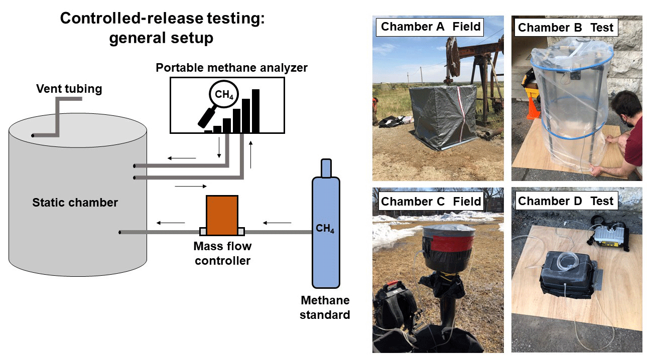
Figure 1 Diagram of the controlled-release experiments for the static chamber method (left), with photos of chamber deployments in both field settings and during controlled-release testing (right). The four chambers shown on the right correspond to the four chambers that we tested.

Mass flow rates were calculated from the rate of methane buildup within the chamber over time multiplied by the volume of the chamber (Eq. 1):

$$\begin{array}{}\text{(1)}& M={\displaystyle \frac{\mathrm{d}c}{\mathrm{d}t}}V,\end{array}$$

where M is the mass flow rate of methane, $\mathrm{d}c/\mathrm{d}t$ is the change in the methane concentration over time, and V is the volume of the chamber.

For some experiments, the methane concentrations within the chamber were expected to rapidly reach steady state. Steady state is reached when the methane concentrations no longer increase over time in the chamber and the concentration of methane within the chamber is equal to the concentration of the released gas. The residence time, or the time to reach steady state, is defined by Eq. (2):

$$\begin{array}{}\text{(2)}& \mathit{\tau }={\displaystyle \frac{V}{Q}},\end{array}$$

where τ is the residence time, V is the volume of the chamber, and Q is the volumetric flow rate of gas (i.e., methane and balance gas combined) into the chamber. For any controlled releases where the expected residence time was 2 min or shorter, we only used the initial 10 data points for the linear regression to avoid the period of exponential decay as methane concentrations approach steady state (Pihlatie et al., 2013).

We summarized the results of the controlled-release tests by calculating the percentage deviation of the true versus measured methane flow rate (Eq. 3):

$$\begin{array}{}\text{(3)}& E={\displaystyle \frac{Q_i-Q}{Q}}\times \mathrm{100},\end{array}$$

where E is the error (in %), Q_i is the estimated methane flow rate, and Q is the actual methane flow rate. For each factor being investigated, we grouped the results depending on whether the measurement was an under- or overestimate of the true methane flow rate. We calculated the accuracy of measurements as a range spanning from the median of the over- and underestimated methane flow rates, respectively. We determined the bias of measurements as the average of the raw percentage errors to determine whether tests were biased more towards the under- or overestimation of methane flow rates.

3 Results

3.1 Prior controlled methane releases and component-level methane emissions

We compiled a total of 1142 component-level methane emission factors from the IPCC Emission Factor Database (IPCC EFDB, 2022). A total of 718 emission factors were from the AFOLU sector, 291 were from the energy sector, and 133 were from the waste sector. The emission factors ranged from 9.8×10⁵ to $-\mathrm{1.1}\times {\mathrm{10}}^{-\mathrm{2}}$ g h⁻¹. We found that 1 % of emission factors were above 100 g h⁻¹, 5 % of emission factors were above 10 g h⁻¹, and 45 % of emission factors were above 1 g h⁻¹. The remaining 55 % of emission factors were below 1 g h⁻¹. Within the energy sector, the highest component-level emission factors were associated with the liquid unloading of storage tanks, flowback events for unconventional oil and gas wells, and fugitive emissions from flaring and venting at oil and gas wells which ranged from 9.8×10⁵ to 1.6×10⁵ g h⁻¹. For the waste sector, the highest component-level emission factors were associated with leachate collection wells, pump stations, and sludge pits from landfills which ranged from 4.3×10³ to 2.4×10³ g h⁻¹. For the AFOLU sector, no component-level emission factors were above 100 g h⁻¹, but the highest component-level methane emissions that we observed from the AFOLU sector were from enteric fermentation from dairy cattle, which emitted at approximately 10 g h⁻¹ (Fig. 2).

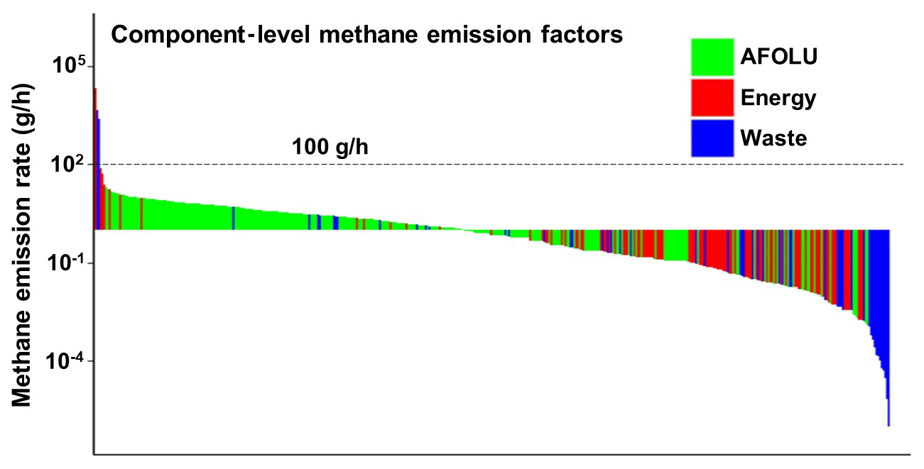
Figure 2 Component-level methane emission factors from the IPCC Emission Factor Database. Emission factors are categorized according to their respective IPCC source category. All emission factors were converted to methane mass flow rates based on the assumptions outlined in Sect. S1.1 in the Supplement.

We analyzed a total of 40 controlled-release studies spanning from 2011 to 2023 (Fig. 3). We found that 32 of the 40 (i.e., 80 %) controlled-release tests had upper methane emission ranges that exceeded 1000 g h⁻¹, with the highest tested flow rate at 7.2×10⁶ g h⁻¹ for a satellite-based platform (Sherwin et al., 2023). We also saw that 31 of the 40 (i.e., 78 %) controlled-release tests had a lower methane emission range that exceeded 100 g h⁻¹. The majority of controlled releases focused on indirect sampling methods, especially mobile surveys (i.e., 45 %) and crewed aircraft (i.e., 30 %) measurement platforms (Fig. 2). Other indirect methods that were tested less frequently in our review were based on uncrewed aircraft (i.e., 15 %), stationary towers (i.e., 13 %), and satellites (i.e., 5 %). For direct measurement methods, we observed that camera-based methods were tested the most frequently (i.e., 10 %). We only found three studies that conducted controlled methane releases for chamber-based methodologies (Riddick et al., 2022; Pihlatie et al., 2013; Christiansen et al., 2011). We found that eight studies performed controlled releases using multiple measurement methods, with two studies (Singh et al., 2021; Riddick et al., 2022) employing five different methodologies. Overall, we found that the majority of controlled-release tests that we analyzed focused on indirect sampling methods and tested methane emissions ≥100 g h⁻¹. Therefore, the testing that we present here (1.02 to 512 g h⁻¹) fills this gap and provides guidance for measuring an appropriate range of component-level methane sources.

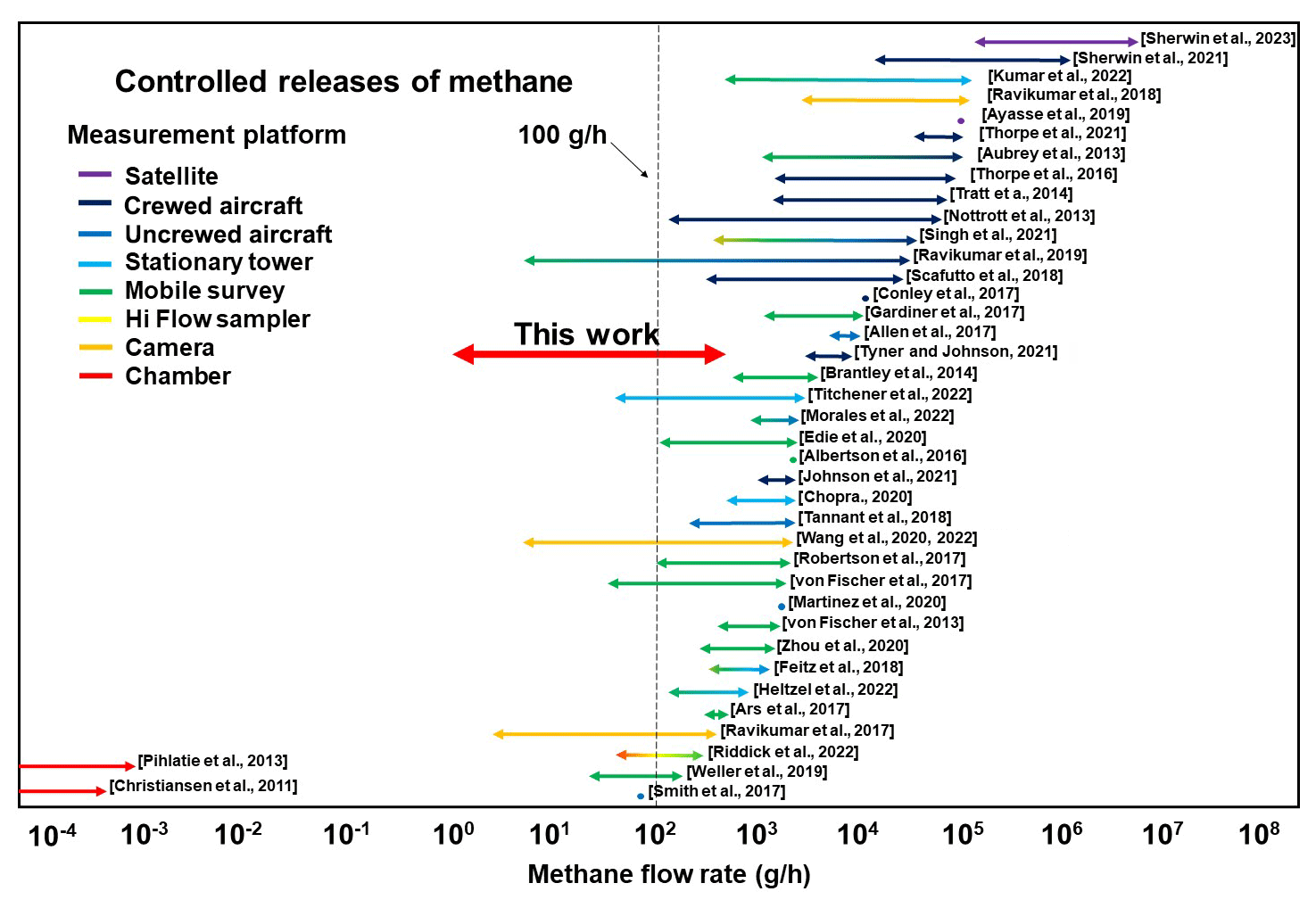
Figure 3 A summary of published literature on controlled releases of methane, showing the range of methane emissions being tested and color-coded according to the measurement platform used to quantify emissions.

3.2 Controlled releases of methane

The accuracy of our 64 controlled-release experiments was $+\mathrm{14}/-\mathrm{14}$ % with a standard deviation of 19 %. The average absolute percentage error was ±20 %, and the median absolute percentage error was ±14 %. The lowest error that we observed was 0.2 %, and 25 of 64 controlled-release tests (i.e., 39 %) had percentage errors lower than ±10 %. Based on testing for bias, we found the average percentage difference between actual and measured mass flow rates to be −3 %, implying a small bias towards the underestimation of methane flow rates.

3.2.1 Chamber volume

Our analysis of chamber volume with respect to the quantification accuracy showed that the accuracy of measurements increased with smaller chamber volumes (Fig. 4). The ≤20 L chambers had the highest accuracy at $+\mathrm{12}/-\mathrm{12}$ % with an error standard deviation of 12 %. The 322 L chamber had a lower accuracy of $+\mathrm{15}/-\mathrm{17}$ % with a standard deviation of 23 %. Our highest errors were measured from the largest 2265 L chamber with an accuracy of $+\mathrm{50}/-\mathrm{16}$ % and a standard deviation of 26 %. We analyzed all three chamber sizes for bias and found that the ≤20 L chambers showed a slight tendency towards the underestimation of flow rates with an average bias of ≥0 %, the 322 L chamber showed a stronger tendency towards the underestimation of flow rates at −18 %, and the 2265 L chamber showed a slight bias towards the overestimation of flow rates at +7 % (Fig. 4).

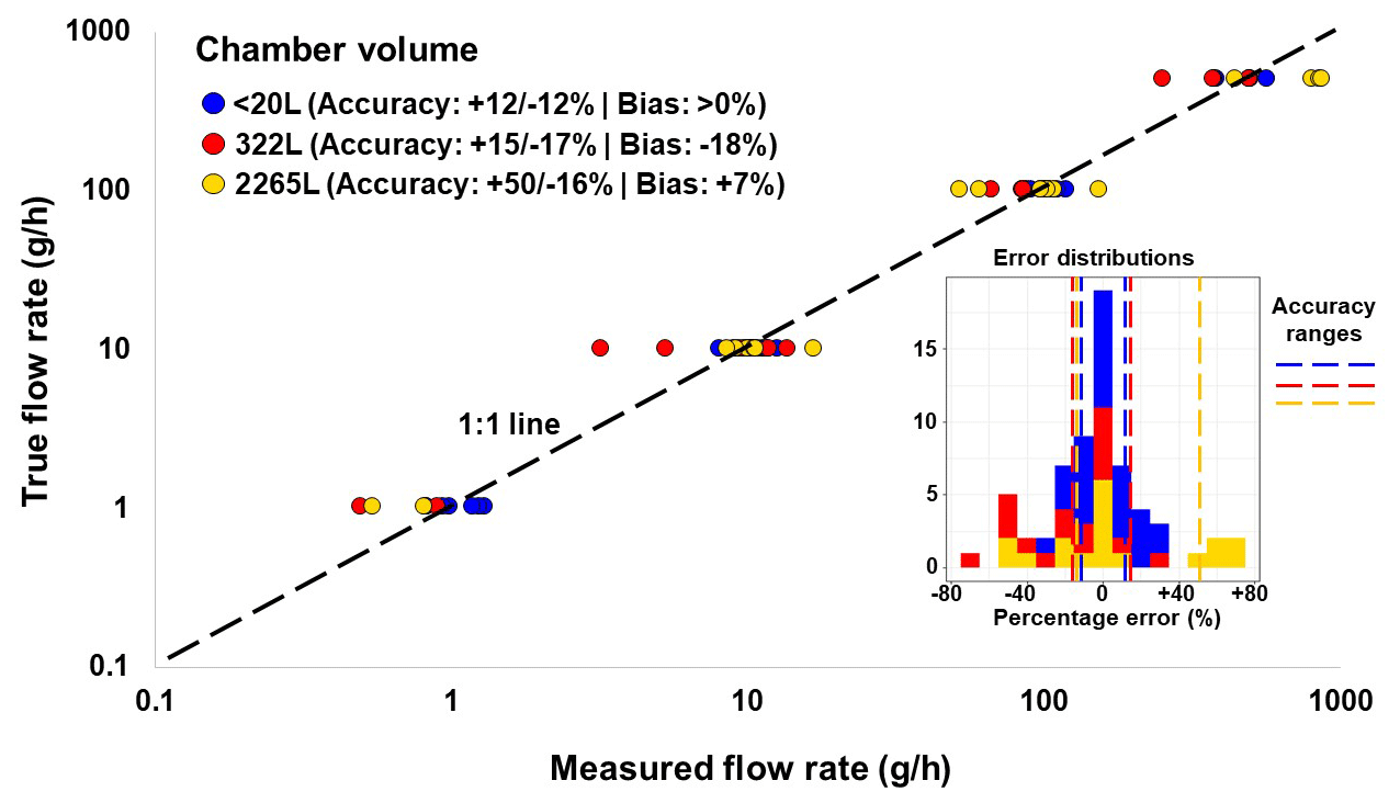
Figure 4 Parity plot showing the true versus measured methane flow rates for different chamber volumes. The distribution of actual percentage errors is shown on the right. Points and bars are color-coded according to the different chamber volumes. A perfect fit is shown by the dashed black line.

3.2.2 Chamber shape

Our comparisons of different chamber shapes showed that the cylindrical chambers were more accurate than the rectangular chambers, with an accuracy of $+\mathrm{5}/-\mathrm{14}$ % and a standard deviation of 18 % (Fig. 5). We found that the rectangular chambers showed a lower accuracy of $+\mathrm{17}/-\mathrm{14}$ % with a standard deviation of 22 %. Similar to the chamber volume, the median percentage error was smaller than the average error for both chamber shapes, indicating an extreme distribution in percentage errors. We analyzed both chamber shapes for bias and found that the cylindrical chambers were biased towards the underestimation of methane flow rates, with an average bias of −13 %, whereas the rectangular chambers showed a small bias towards the overestimation of methane flow rates, with an average bias of +6 % (Fig. 5).

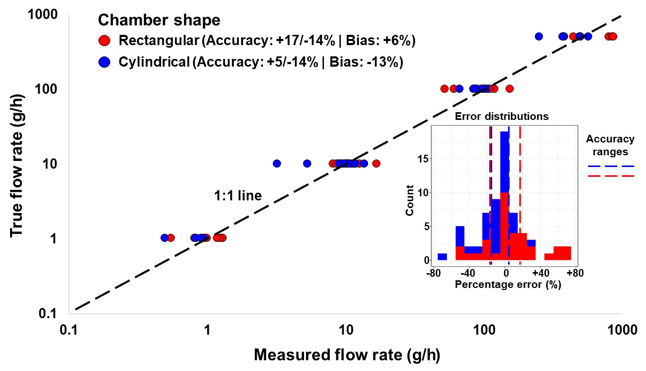
Figure 5 Parity plot showing the true versus measured methane flow rates for different chamber shapes. The distribution of actual percentage errors is shown on the right. Points and bars are color-coded according to the different chamber shapes. A perfect fit is shown by the dashed black line.

3.2.3 Use of fans

The most impactful physical factor that we observed on chamber measurement accuracy was the presence of fans. Chambers with fans present had a median percentage error of $+\mathrm{6}/-\mathrm{5}$ % and a standard deviation of 17 % (Fig. 6), which was higher than chambers without fans that had an accuracy of $+\mathrm{17}/-\mathrm{17}$ % and a standard deviation of 22 %. For both datasets, we observed median values lower than the mean, indicating a skewed dataset. We analyzed both datasets for bias and found that chambers with and without fans both showed slight biases towards the underestimation of methane flow rates at −2 % and −4 %, respectively (Fig. 6).

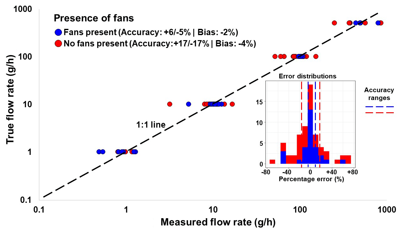
Figure 6 Parity plot showing the true versus measured methane flow rates for experiments with and without the presence of fans. The distribution of actual percentage errors is shown on the right. Points and bars are color-coded according to whether fans were present or not. A perfect fit is shown by the dashed black line.

3.3 The effects of leak properties

3.3.1 Mass flow rate

We tested four different mass flow rates for our controlled-release tests: 1.02, 10.2, 102, and 511 g h⁻¹ (Fig. 7). The lowest errors were measured from the 10.2 and 102 g h⁻¹ mass flow rates, with accuracies of $+\mathrm{8}/-\mathrm{11}$ % and $+\mathrm{7}/-\mathrm{13}$ %, respectively. The lowest accuracy of $+\mathrm{56}/-\mathrm{15}$ % was attributed to the highest mass flow rate of 512 g h⁻¹. We found that the 1.02, 10.2, and 102 g h⁻¹ mass flow rates all had negative biases of −11 %, −1 %, and −6 %, respectively. The mass flow rate of 512 g h⁻¹ had a slight bias of +4 % towards the overestimation of mass flow rates and also had the highest upper accuracy estimate of +46 % that we observed among the different factors analyzed.

3.3.2 Volumetric flow rate

We analyzed six different volumetric flow rates for the range of methane flow rates that we tested: 0.238, 0.476, 2.38, 4.76, 11.9, and 23.8 L min⁻¹ (Fig. 7). We found that the lowest accuracies were attributed to both the highest and lowest volumetric flow rates (with accuracies of $+\mathrm{50}/-\mathrm{15}$ % and $+\mathrm{21}/-\mathrm{14}$ %, respectively), whereas higher accuracy was observed with the mid-level volumetric flow rates of 11.8, 4.76, 2.38, and 0.476 slpm (with accuracies ranging from $+\mathrm{26}/-\mathrm{3}$ % to $+\mathrm{9}/-\mathrm{11}$ %). Similar to the mass flow rates, we also found that the highest accuracies were associated with the mid-level volumetric flow rates, whereas the lowest accuracies were observed at the upper and lower volumetric flow rates.

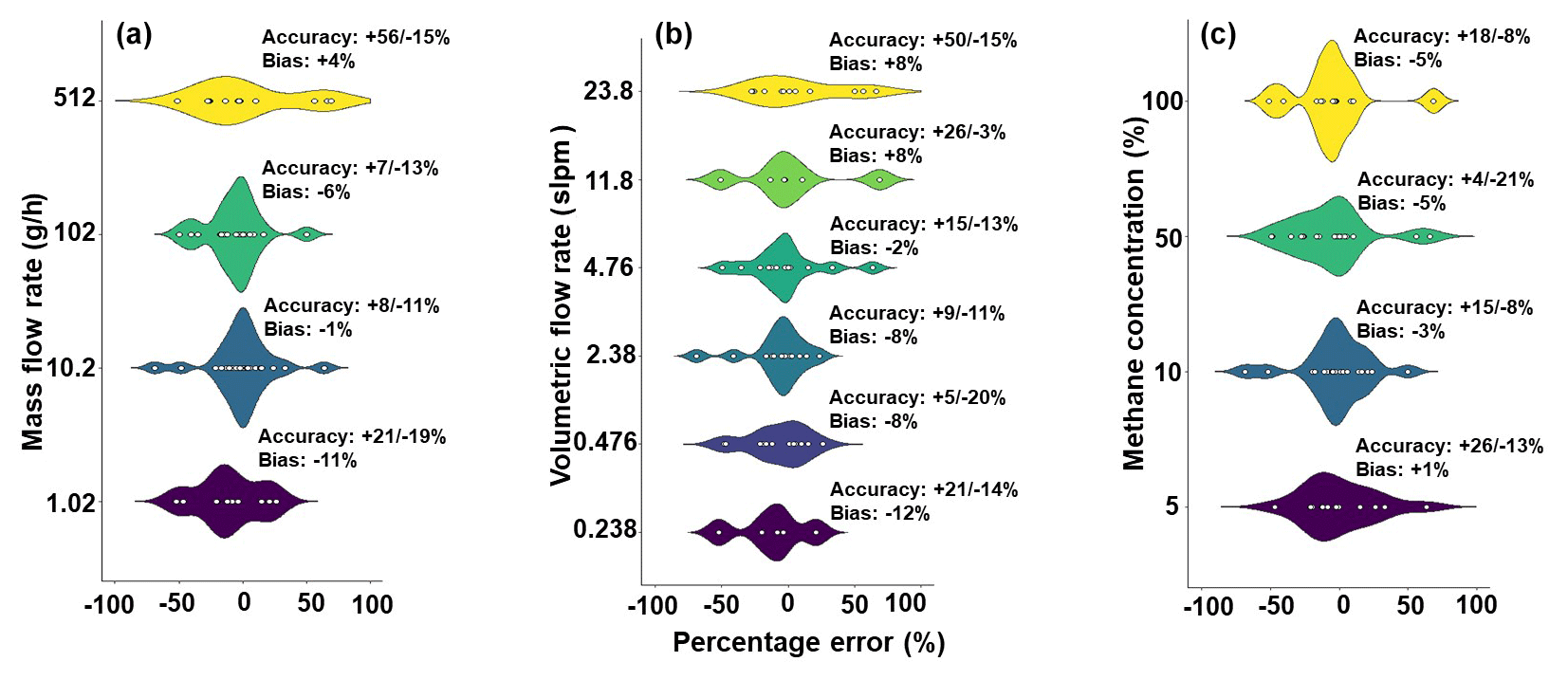
Figure 7 Violin plots of the percentage errors of the true versus measured methane flow rates under varying mass flow rates (a), volumetric flow rates (b), and gas concentrations (c) of methane. The points represent the measured percentage errors, and the shaded areas represent the relative density (on the y axis) of the observed percentage errors. Uncertainty ranges and biases are displayed for each factor.

3.3.3 Methane percentage of leaking gas

We analyzed four different percentages of methane in the leaking gas for the controlled releases (Fig. 7). The lowest accuracies were associated with the 5 % methane gas with an accuracy of $+\mathrm{31}/-\mathrm{16}$ %, whereas the highest accuracies were observed with the 10 % methane at $+\mathrm{15}/-\mathrm{8}$ %. The three highest percentages of methane in the leaking gas all had small negative biases ranging from −5 % to −3 %, whereas the 5 % methane leak had a slight positive bias at +1 %.

3.4 Optimizing the static chamber method for accuracy

For consistency, we define release rates of 1.02 and 10.2 g h⁻¹ as low flow rates, whereas release rates of 102 and 512 g h⁻¹ are defined as high flow rates. In addition, we define chamber volumes ≤20 L as small and chamber volumes of 322 and 2265 L as large. We analyzed how chamber configurations (i.e., chamber volume, the use of fans, and chamber shape) can be optimized to increase the accuracy of methane flow rate estimates. In general, we found that smaller chambers produced the lowest errors. No measurements from smaller chambers produced a percentage error above ±30 %. We also saw that smaller chambers performed similarly regardless of the presence of fans, with smaller chambers with fans producing an accuracy of $+\mathrm{16}/-\mathrm{8}$ % and smaller chambers without fans having an accuracy of $+\mathrm{12}/-\mathrm{13}$ %. Smaller chambers performed slightly better if the chambers were cylindrical, with an accuracy of $+\mathrm{3}/-\mathrm{12}$ % compared with smaller rectangular chambers that had an accuracy of $+\mathrm{16}/-\mathrm{3}$ %. For larger chambers (i.e., ≥20 L), the use of fans was critical for reducing measurement error. Larger chambers with fans produced an accuracy of $+\mathrm{4}/-\mathrm{5}$ % compared with large chambers without fans that produced an accuracy of $+\mathrm{63}/-\mathrm{27}$ %. Therefore, although smaller chambers generally had lower errors than larger chambers, the errors in the larger chambers could be comparable to the smaller chambers when fans were used.

We found that chamber configurations could also be optimized according to the mass flow rate of methane. At low mass flow rates of methane (i.e., ≤100 g h⁻¹), we found that smaller chambers were more accurate than larger chambers, with accuracies of $+\mathrm{12}/-\mathrm{8}$ % and $+\mathrm{15}/-\mathrm{19}$ %, respectively. The use of fans had little impact on the accuracy of smaller chambers at these low flow rates, with smaller chambers with fans producing an accuracy of $+\mathrm{16}/-\mathrm{8}$ % and smaller chambers without fans having an accuracy of $+\mathrm{7}/-\mathrm{13}$ %. In contrast, the use of fans was important for the accuracy of larger chambers at these lower mass flow rates. Larger chambers with fans had an accuracy of $+\mathrm{4}/-\mathrm{30}$ %, whereas larger chambers without fans had an accuracy of $+\mathrm{48}/-\mathrm{19}$ %. In terms of the chamber shape, at low flow rates, smaller cylindrical chambers had an accuracy of $+\mathrm{1}/-\mathrm{11}$ % compared with small rectangular chambers that produced an accuracy of $+\mathrm{15}/-\mathrm{3}$ %. For larger chambers at low mass flow rates, we observed a contrasting result with large rectangular chambers producing an accuracy of $+\mathrm{6}/-\mathrm{16}$ % and large cylindrical chambers producing a median percentage error of $+\mathrm{24}/-\mathrm{48}$ %.

We observed similar results when optimizing chamber configurations for high methane mass flow rates (i.e., ≥100 g h⁻¹). We found that smaller chambers (≤20 L) performed better than larger chambers, with accuracies of $+\mathrm{14}/-\mathrm{13}$ % and $+\mathrm{50}/-\mathrm{16}$ %, respectively. We also found that the use of fans was critical for measurement accuracy for larger chambers at higher mass flow rates of methane. Larger chambers with fans had an accuracy of $+\mathrm{4}/-\mathrm{4}$ % compared with larger chambers without fans that had an accuracy of $+\mathrm{66}/-\mathrm{35}$ %. With respect to chamber shapes, cylindrical chambers were more accurate than rectangular chambers, with an accuracy of $+\mathrm{6}/-\mathrm{14}$ % compared with $+\mathrm{26}/-\mathrm{15}$ %, respectively. At higher mass flow rates of methane, we found that large cylindrical chambers with fans were highly accurate at $+\mathrm{2}/-\mathrm{3}$ % of the true methane flow rate.

From all of the controlled-release experiments that we performed, we saw that the median absolute error of ±14 % was lower than the mean error of 20 %, indicating a heavy-tailed distribution of measurement errors. As such, we analyzed all controlled-release experiments where the resulting error exceeded 40 % in order to assess the potential cause of these erroneous measurements. A total of 12 controlled releases had quantification errors that exceeded 40 % (Fig. S1 in the Supplement). All of these experiments were conducted on larger-volume chambers (i.e., 322 and 2265 L), and 8 of the 12 had no fans present. Based on a comparison of the fit of the linear regressions, we found that these 12 experiments did have a good correlation between the methane concentrations and time, with R² values averaging 0.91 when compared to the rest of the dataset (mean R²=0.96). Notably, 3 of the 12 high-error measurements had very high R² values exceeding 0.99, with an example being shown in the bottom left panel of Fig. 8. We observed a similar phenomena with a single controlled-release performed with an “ideal” and “nonideal” chamber seal (shown in Sect. S1 in the Supplement), where a nonideal chamber seal produced a high R² value but underestimated the methane flow rate by 43 %.

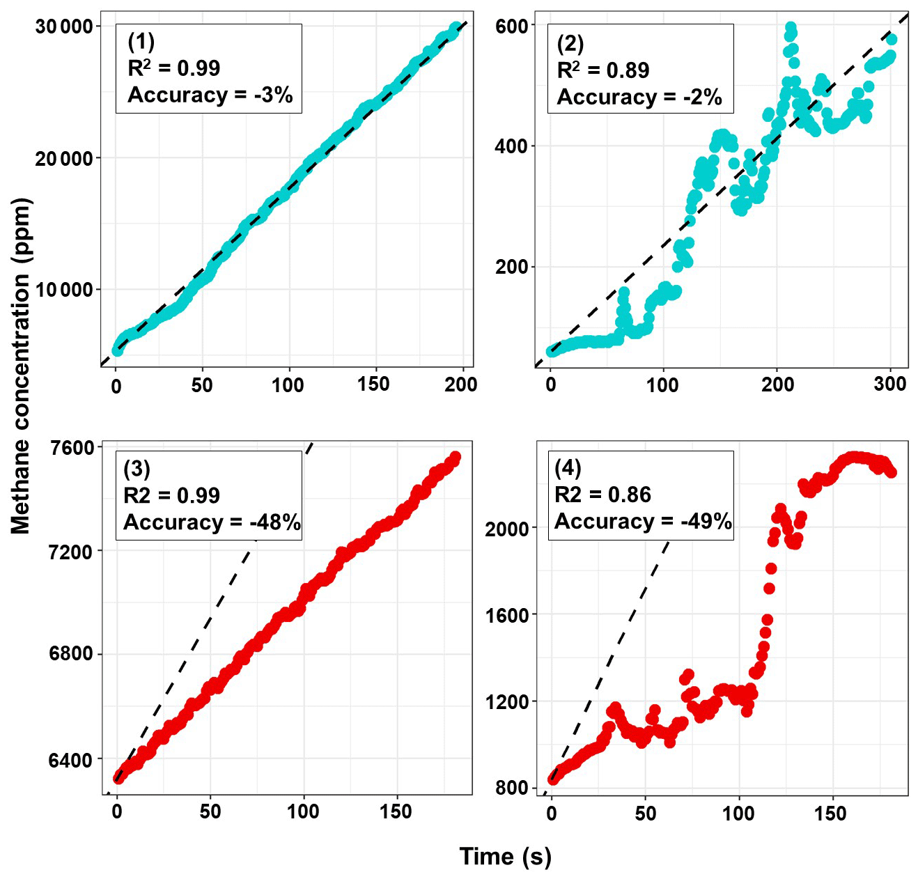
Figure 8 Four examples of raw controlled-release data showing methane concentrations versus time. The measured concentrations within the chamber are shown by the colored dots, and the true or expected concentrations are indicated by the dashed lines. Points colored blue indicate a measurement error less than 40 %, and the points colored red indicate a measurement error greater than 40 %. The examples shown are (1) high R² value and high quantification accuracy, (2) low R² value and high quantification accuracy, (3) high R² value and low quantification accuracy, and (4) low R² value and low quantification accuracy.

4 Discussion

Our compilation of component-level methane flow rates from the IPCC Emission Factor Database showed that 99 % of the component-level emission rates fall below the 100 g h⁻¹ level. Therefore, it is important to develop and test methane quantification methods for these lower methane flow rates (i.e., ≤100 g h⁻¹). Quantification of methane emissions at the component level provides a level of detail necessary to develop actionable mitigation strategies through the clear identification of emitting components. Most controlled-release studies focus on indirect sampling methods which are effective in measuring methane emissions at the site- and/or facility-level scale. While these data are important for validating greenhouse gas inventories and quantifying emissions from super-emitting methane sources (Brandt et al., 2016; Ravikumar et al., 2017), emissions data at the component level are also needed to improve bottom-up greenhouse gas inventories and develop actionable mitigation strategies. Many of the component-level sources that we consider, such as sewage utility holes, livestock, abandoned oil and gas wells, and NG pipeline leaks, have been shown to be significant methane sources at municipal; provincial, state, or territorial; or national levels (Williams et al., 2022, 2020; El Hachem and Kang, 2022; Seiler et al., 1983; Kang et al., 2016; Hendrick et al., 2016). These sources are all characterized by low methane emission rates (below 100 g h⁻¹ on average) that are challenging to measure using indirect methods. Several studies have highlighted the super-emitting nature of methane emission sources, particularly from the NG sector (Brandt et al., 2016). However, the upper range of super-emitting methane sources varies depending on the source being measured. For example, a study of methane emissions from Montréal, Canada, found that both residential NG meter sets and sewage utility holes were significant sources of methane for the city, despite having maximum methane emission rates of 4.2 and 33 g h⁻¹, respectively (Williams et al., 2022). While many controlled-release studies focus on a higher range of methane emissions, it is still important that methods are developed and tested for lower methane emission sources.

In addition to the factors that we tested, there are several other sources of uncertainty in the static chamber method that we did not investigate. One factor that could impact measurement accuracy is the effectiveness of the chamber seal. An improper chamber seal could lead to the intrusion of atmospheric air, which dilutes the chamber headspace and leads to an underestimation of the true methane flow rate (Sect. S1). Typically, in field settings, chambers are sealed to the ground (Kang et al., 2016; Lebel et al., 2020). In some cases, chambers can be sealed aboveground to an emitting component. A variety of different methods have been used to create these chamber-to-site seals, such as tape, bungee cords, chamber collars, sand, and snow (Williams et al., 2020; Lebel et al., 2020; Kang et al., 2016). In our experience, smaller chambers are easier to seal to an emitting component, given the smaller size and ease of identifying potential breaches. Ensuring a proper chamber seal in larger chambers is more difficult due to the chamber size, but it is achievable under stable environmental conditions. The methane concentration measurement method is one aspect of the static chamber method that will affect both the measurement accuracy and sensitivity of the static chamber method. In this work, we use a portable greenhouse gas analyzer to continuously measure methane concentrations within the chamber. Uncertainty related to the frequency of methane concentration measurement and the accuracy and precision of the greenhouse gas analyzer are all important factors related to uncertainty. Furthermore, portable greenhouse gas analyzers can generally be classified as either measuring a full range of methane concentrations at the cost of precision at lower methane concentrations (i.e., ≤10 ppm methane) or measuring methane with high precision at the cost of an upper measurement range (i.e., 1000 ppm). Therefore, the selection of the greenhouse analyzer can also be optimized according to the methane source being measured to improve accuracy. Other factors such as the release point of the emitted gas, the presence of multiple emission sources, the environment, the chamber rigidity, the method and strength of interior chamber mixing, and the position of the gas sampling points are all factors that could also impact measurement uncertainty. Further analysis of the impacts of these factors on measurement accuracy would be beneficial for guiding the ideal deployment of the static chamber method for the quantification of component-level methane sources.

Our results showed that the static chamber methodology can quantify methane emissions ranging from 1.02 to 512 g h⁻¹ with an accuracy of $+\mathrm{14}/-\mathrm{14}$ %. In comparison to indirect methods, Johnson et al. (2023) state that their aircraft-based method has a multi-pass uncertainty range of $-\mathrm{46}/+\mathrm{54}$ %, which roughly corresponds to an absolute error of ±50 %. In von Fischer et al. (2017), they state an uncertainty range of $-\mathrm{24}/+\mathrm{32}$ % after five mobile survey passes, which roughly corresponds to an absolute error of ±28 %. With regards to other controlled-release tests on static chambers, we find that our median uncertainty of $+\mathrm{14}/-\mathrm{14}$ % falls within the 10 %–20 % range reported by Lebel et al. (2020) and Pihlatie et al. (2013). For the larger chambers, we find that the use of fans is critical for maximizing accuracy, which is expected given the larger volume of air that is required to be mixed. The 12 largest measurement errors in this work occurred from large volume chambers, with 8 of those controlled releases having no fans present. The larger chambers that we used were all collapsible chambers; this could have impacted the measurement accuracy due to the wind altering the shape of the chamber walls and the chamber volume during the experiment. The large-volume chambers that we used are designed to accommodate the odd site shapes encountered in the field, such as abandoned oil and gas wells (Fig. 1). Future controlled-release studies that test larger-volume rigid chambers would help elucidate the cause of these high errors. We also noted that all of these large-measurement-error experiments showed high R² values above 0.80, meaning that they would be difficult to distinguish based on the goodness of fit of the measurement data alone. Furthermore, several experiments showed relatively poor R² values but good measurement accuracy (Fig. 8), adding to this difficulty. We found that chamber shape is more important for larger chambers than for smaller chambers, with the large, cylindrical chamber performing better than the large, rectangular chamber, whereas we did not find any difference between the smaller chambers with respect to shape. Ideally static chambers should be constructed to minimize potential dead zones where gases can accumulate (Christiansen et al., 2011), and cylindrical, or even semispherical or spherical chambers, should facilitate easier mixing of the chamber headspace.

At higher methane flow rates (≥100 g h⁻¹), we found that our large cylindrical chamber with fans quantified methane emissions with the highest accuracy (i.e., $+\mathrm{2}/-\mathrm{3}$ %) of any chamber combination used throughout this study. In addition, a methane source such as an oil or gas well can have multiple emitting components (e.g., pipe flanges, valves, surface casing vents, and soil gas migration) that could be missed when using smaller chambers. Methane concentrations within a smaller chamber can also rapidly reach explosive levels which can pose safety concerns if the environment is not intrinsically safe (Riddick et al., 2022); however, these risks can be minimized at little cost to accuracy if fans are omitted. Furthermore, intrinsically safe methods of chamber mixing, such as external pumps, could be used to mix air within chambers, regardless of the size of chamber. Theoretically, there is no upper methane flow rate limitation for the static chamber method, and utilizing large chambers, such as the 32 000 L chamber used in Lebel et al. (2020), could theoretically quantify methane flow rates in the 100–200 kg h⁻¹ range. However, there are practical limitations to directly measuring components emitting methane at these high levels, with the most notable being safety concerns and access issues (e.g., measuring flare stacks and liquid storage tank unloading). Another factor to consider is the time to reach steady state. Enclosing a high-methane-emission source within a smaller chamber causes methane concentrations within the chamber to rapidly reach steady state, essentially creating a dynamic chamber, which we do not test in this work (Pedersen et al., 2010; Levy et al., 2011). Overall, our findings indicate that small chambers (i.e., ≤20 L), regardless of the chamber shape or use of fans, can be used to quantify component-level methane flow rates with an accuracy of ±11 % for methane flow rates ranging from 1.02 to 512 g h⁻¹. If larger chambers are required/desired, optimal configurations (i.e., fans present and cylindrical shapes) will produce errors of ±3 % for high methane flow rates (i.e., ≥100 g h⁻¹).

5 Conclusions

Our results have shown that the static chamber methodology can be an effective and accurate method for the quantification of component-level methane flow rates. Whereas indirect sampling methods have been extensively tested, there is a need to test direct sampling methods given their ability to quantify methane emissions at the component level, which is important for developing actionable mitigation strategies. The static chamber method is logistically simple to implement and adaptable to multiple methane sources, making it a viable measurement option for many component-level emission sources. Going forward, there are opportunities to improve the static chamber design in order to reduce measurement uncertainties. Our work provides the testing and design information for the static chamber methodology, thereby contributing to the range of measurement tools needed to quantify methane emission rates from all sources.