the Creative Commons Attribution 4.0 License.
the Creative Commons Attribution 4.0 License.
 | 25 Jul 2023
Detecting plumes in mobile air quality monitoring time series with density-based spatial clustering of applications with noise
Blake Actkinson
Robert J. Griffin
Mobile monitoring is becoming an increasingly popular technique to assess air pollution on fine spatial scales, but methods to determine specific source contributions to measured pollutants are sorely needed. One approach is to isolate plumes from mobile monitoring time series and analyze them separately, but methods that are suitable for large mobile monitoring time series are lacking. Here we discuss a novel method used to detect and isolate plumes from an extensive mobile monitoring data set. The new method relies on density-based spatial clustering of applications with noise (DBSCAN), an unsupervised machine learning technique. The new method systematically runs DBSCAN on mobile monitoring time series by day and identifies a subset of points as anomalies for further analysis. When applied to a mobile monitoring data set collected in Houston, Texas, analyzed anomalies reveal patterns associated with different types of vehicle emission profiles. We observe spatial differences in these patterns and reveal striking disparities by census tract. These results can be used to inform stakeholders of spatial variations in emission profiles not obvious using data from stationary monitors alone.
- Article
(3803 KB) - Full-text XML
-
Supplement
(1955 KB) - BibTeX
- EndNote


A central question of air pollution studies is to identify the varied sources that contribute to measured pollutant concentrations. This question becomes more complicated in a mobile monitoring context because measurements and concentrations vary as a function of both space and time, making conventional source apportionment techniques such as positive matrix factorization and principal component analysis (PCA) harder to apply effectively (Larson et al., 2017).
Recently published work took several approaches to performing source apportionment on measured pollutants in a mobile monitoring context. One approach involves using PCA on background subtracted measurements, such as in Larson et al. (2017), whose approach has limitations when applied to extensive mobile monitoring campaigns because it defines a rolling minimum across a static time window that may not be applicable for extensive mobile monitoring campaigns with ≈ 20–30 × the temporal coverage. Other approaches have focused on using land use regression (LUR) models to identify relationships between pollutants and land use variables, such as in Messier et al. (2018). However, LUR models require spatiotemporal databases of sufficient temporal and spatial resolution for use in model training. While recent efforts have illustrated creative methods of creating these land use databases (Qi and Hankey, 2021), use of these models is still limited through the availability of these databases. There is a need for the development of methods that can identify source influences in large mobile monitoring data sets at high time resolution without being subject to the availability of land use variable databases.
Another factor that aggravates source identification in mobile monitoring contexts is the nature of mobile monitoring data themselves. If a mobile monitoring campaign were conducted focusing largely on residential areas with brief excursions into traffic-congested areas, such as highways, performing PCA or other dimension reduction techniques to describe patterns in the entire data set would likely return results that are weighted towards residential areas with negligible source influences. This type of analysis generates solutions in which there is a demarcation between a majority of points with little source influence and a smaller subset of source-influenced points elevated in all pollutants, which is not compelling if the objective is to determine the specific sources affecting the measurements.
This raises the question of how to identify source influences within mobile monitoring time series that cover locations ranging from “background” to “highly influenced by sources”. If one could identify source spikes or plumes within mobile monitoring time series, one could restrict their analysis to these plumes to categorize the different types of sources that affected their mobile monitoring measurements. Plume identification within mobile monitoring time series has been addressed previously. Hagler et al. (2012) use a rolling coefficient of variation across a 5 s time interval and then flag points with a coefficient greater than 2. Drewnick et al. (2012) use a different moving window algorithm that calculates the standard deviation of points below a defined background threshold (σb) and flags points which are more than 3σb above the previous point. The algorithm then flags subsequent points, increasing the threshold necessary (by a factor of , in which nf is the total number of flagged points) for flagging for every subsequent point beyond the first flagged point. Others have addressed the plume identification question indirectly through background estimation and removal methods.
These methods all have drawbacks. In the data used in the present work, the method of Hagler et al. (2012) flags few to no points at all, suggesting that the method is sensitive to the time series utilized. The algorithm of Drewnick et al. (2012) suffers in situations where many plumes appear consecutively to one another, frequently leading to poor performance in those circumstances. Other methods depend on a time window, which presents problems for complex, multi-day mobile monitoring time series.
Here we discuss an algorithm to identify plumes in a different manner. The algorithm relies on density-based spatial clustering of applications with noise (DBSCAN), a nearest-neighbor clustering algorithm (Ester et al., 1996). DBSCAN clusters points based on whether they fall into predetermined neighborhoods with other points. The technique can cluster points with more complicated shapes (e.g., an “S” embedded in noise in two-dimensional space) and is not sensitive to starting values compared to other clustering techniques such as k means (Tan et al., 2019). Additionally, the algorithm does not require every single point to be clustered, allowing for those points that do not neatly fall into a given cluster to be defined as noise.
The objective of this work is to establish a new method for detecting plumes in mobile monitoring time series, validate its performance, and use it to perform novel analysis that elucidates the impacts of different emission sources across census tracts in the Greater Houston area. We utilize DBSCAN by envisioning daily mobile monitoring time series collected in Houston (Miller et al., 2020; Actkinson et al., 2021) that include black carbon (BC), carbon dioxide (CO2), oxides of nitrogen (nitric oxide (NO) + nitrogen dioxide (NO2) = NOx), and ultrafine particle (UFP) number concentrations as large numbers of points clustered around a four-dimensional origin with plumes scattered outwards from this origin. In the DBSCAN context, plumes would be labeled as noise. We first describe DBSCAN and then detail how we adapt it for application to mobile monitoring time series. To evaluate performance, we construct a validation set by manually flagging plumes via visual inspection from a randomly chosen subset of days from the Houston mobile monitoring campaign (Miller et al., 2020; Actkinson et al., 2021). We use the validation set to tune DBSCAN and other time-series-based models and compare the performance of all models. We apply the algorithm to the Houston mobile monitoring data set to identify anomalies, which are then clustered into anomaly types linked to specific vehicle emission sources. We tabulate the number of these different anomaly types by census tract and derive anomaly frequencies, which are conceptualized as the probability of detecting a given anomaly type during the prescribed study period. We demonstrate differences in anomaly frequencies in census tracts across Houston, which can be used to tailor census-tract-specific air monitoring regulation and enforcement strategies. We discuss the implications of the method, the results, and future directions for this research.
2.1 Data
Data were collected during the Houston mobile monitoring campaign and are described in detail elsewhere (Miller et al., 2020; Actkinson et al., 2021). The campaign's objective was to measure air pollution on a very fine spatial scale in 35 different census tracts across the Greater Houston area in a 9-month time span. Two Google Street View cars were driven through these census tracts systematically to evaluate spatial differences in the concentrations of seven pollutants. Previous analyses with this data set focused on identifying large concentrations attributable to sources along specific individual roadways and on developing a technique to identify and remove background concentrations from the time series collected (Miller et al., 2020; Actkinson et al., 2021).
In the current analysis, we restrict the set of analyzed pollutants to be BC, CO2, UFP, and NOx. Here, we do not consider fine particle mass (PM2.5) concentration and ozone due to the influence of secondary processes. Table S1 in the Supplement provides the instruments used to measure each respective pollutant. BC, CO2, and UFP measurements were taken on 1 s time resolution, while NO and NO2 measurements were taken on 5 s time resolution. With the addition of logged global positioning system (GPS) coordinates from each car, the campaign generated a massive spatiotemporal data set spanning millions of observations across the 9-month span.
In this work, we create a multivariate data set consisting of the four air pollution variables at 1 s time resolution, along with corresponding latitude and longitude coordinates and timestamps that span 277 separate days of sampling for a total of 5 301 507 observations. The BC data were smoothed with a 10 s time window to limit the effects of noise on subsequent analysis. In the original data set, NO and NO2 were taken on a 5 s time resolution, while CO2, BC, and UFP were all collected at 1 s resolution. To perform analysis at a finer temporal resolution, as well as to address missing data, we use monotone Hermitian splines to impute missing measurements up to a 6 s time gap. While previous mobile monitoring studies have fused 5 s data with 1 s data by repeating the same 5 s measurement each second across the entire interval (Shah et al., 2018; Miller et al., 2020), we argue that using continuous splines provides a more realistic estimate of missing 1 s information in this context. Previous studies have focused on preserving the spatial meaning of concentration plotted on maps at very fine spatial intervals; here, we are more interested in estimating temporal variations in missing concentrations, and splines are suitable tools to do so for brief 6 s intervals. Total imputed percentages for each pollutant were 1.06 %, 80.0 %, 80.0 %, 0.42 %, and 0.49 % for BC, NO, NO2, CO2, and UFP, respectively; 90.1 % of NOx realizations had at least one imputed measurement. Any multivariate realization with at least one missing observation in a variable not imputed was excluded otherwise. Days in which the cars operated had to possess a minimum of 600 measurements to be included in the analysis. Using road shapefiles available through the TigerLINE road database (U.S. Census Bureau, 2018), we assign road categories to each of our points based on their respective latitude and longitude coordinates. To be consistent with Miller et al. (2020) and Actkinson et al. (2021), we restrict our analysis to points with logged latitude and longitude coordinates on primary, secondary, local, and private roads, as well as ramps and service drives, because these are roads typically relevant to an individual's exposure. To account for GPS error, we remove logged GPS coordinates whose nearest-neighbor distance to a TigerLINE shapefile point is more than 30 m. Additionally, we observed evidence of the vehicles sampling their own exhaust when driving to and from dead ends in a previous analysis of the data set (Miller et al., 2020). Because we do not want to characterize our own individual vehicle's emissions, we remove points less than 30 m from a dead end in a road.
2.2 DBSCAN
DBSCAN is a clustering routine originally conceived by Ester et al. (1996). Using two predefined parameters, epsilon (ϵ) and MinPts, DBSCAN seeks to label points that have MinPts points within a neighborhood defined with radius ϵ as core points, points that do not meet the MinPts criteria but have a core point within their ϵ neighborhood as border points, and points that do not fit either of these criteria as noise.
More formally, the ϵ neighborhood around a point p∈D is defined using the notation of Hahsler et al. (2019) as
where N is the neighborhood, D is the set of points, and d is a distance measure such as the Euclidean distance. A point is defined as a core point if
where MinPts is the minimum points parameter and denotes cardinality. The algorithm systematically labels points as core points, border points, or noise points depending on these criteria.
2.3 Validation set construction
To tune parameters and evaluate algorithm performance, we construct a validation set from the mobile monitoring data by manually flagging visible plumes within 30 randomly selected daily mobile monitoring time series (out of a possible total of 277); example validation set data are shown in Fig. S1. The total number of points in the validation set was 564 107, which amounts to ≈ 10 % of the entire set. A graphical user interface in IgorPro was used to flag plumes by visually inspecting the time series for spikes in pollutant concentrations for each pollutant (BC, CO2, NOx, and UFP). Any time series realization that had a spike in at least one pollutant was flagged.
2.4 Algorithm description
We create an algorithm incorporating DBSCAN to label anomalies systematically within the Houston mobile monitoring campaign. Pseudo-code for this algorithm is given in Fig. 1. The algorithm estimates ϵ and MinPts parameters for daily time series in the campaign based on the number of points in each time series and its dispersion and subsequently performs DBSCAN using these estimated parameters. We define the MinPts parameter to be the product of the total number of points in the daily time series, n, and a fractional value parameter, fval. We set fval to 0.03 using the external validation set and describe the specific procedure in Sect. 2.6. We do not consider values of fval greater than 0.5 due to rapidly increasing computational cost and poor performance at higher values. After calculating MinPts, we determine ϵ using a k-nearest-neighbor (knn) distance ordering procedure in which the value of k was set equal to MinPts and in which a point is the kth nearest neighbor to another point if the distance between the two points is the kth shortest distance among all points. We construct an ordered knn distance set and determine the mean and standard deviation of the first 30 ordered distances, and we then define ϵ as the first distance that is greater than the mean plus 3 times the standard deviation of the subset of previously ordered distances. We iterate through the entire set of remaining distances, adding the current distance to the subset if it does not meet the criteria used to define ϵ. Once both ϵ and MinPts are determined, we run DBSCAN on the daily time series observations in which core points are labeled as normal and both border and noise points are labeled as anomalies. An example of labeled DBSCAN output for a scatterplot of daily BC CO2 time series is given in Fig. 2.
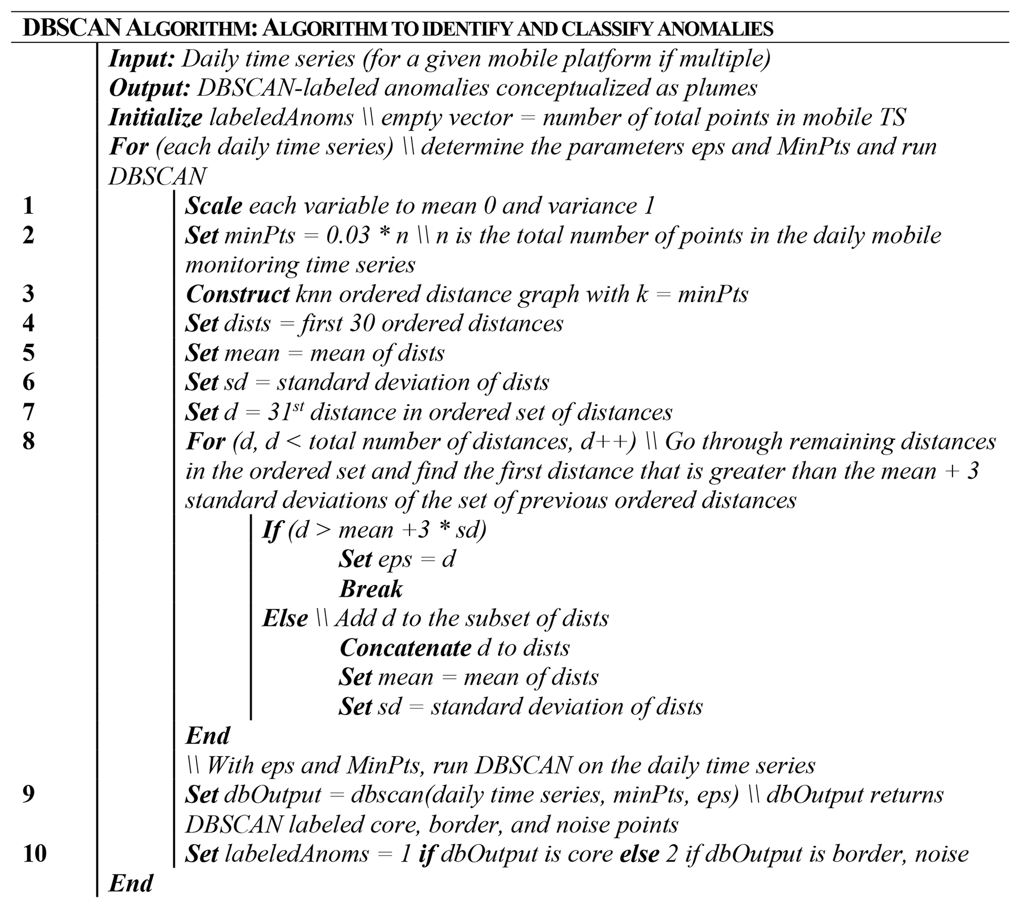
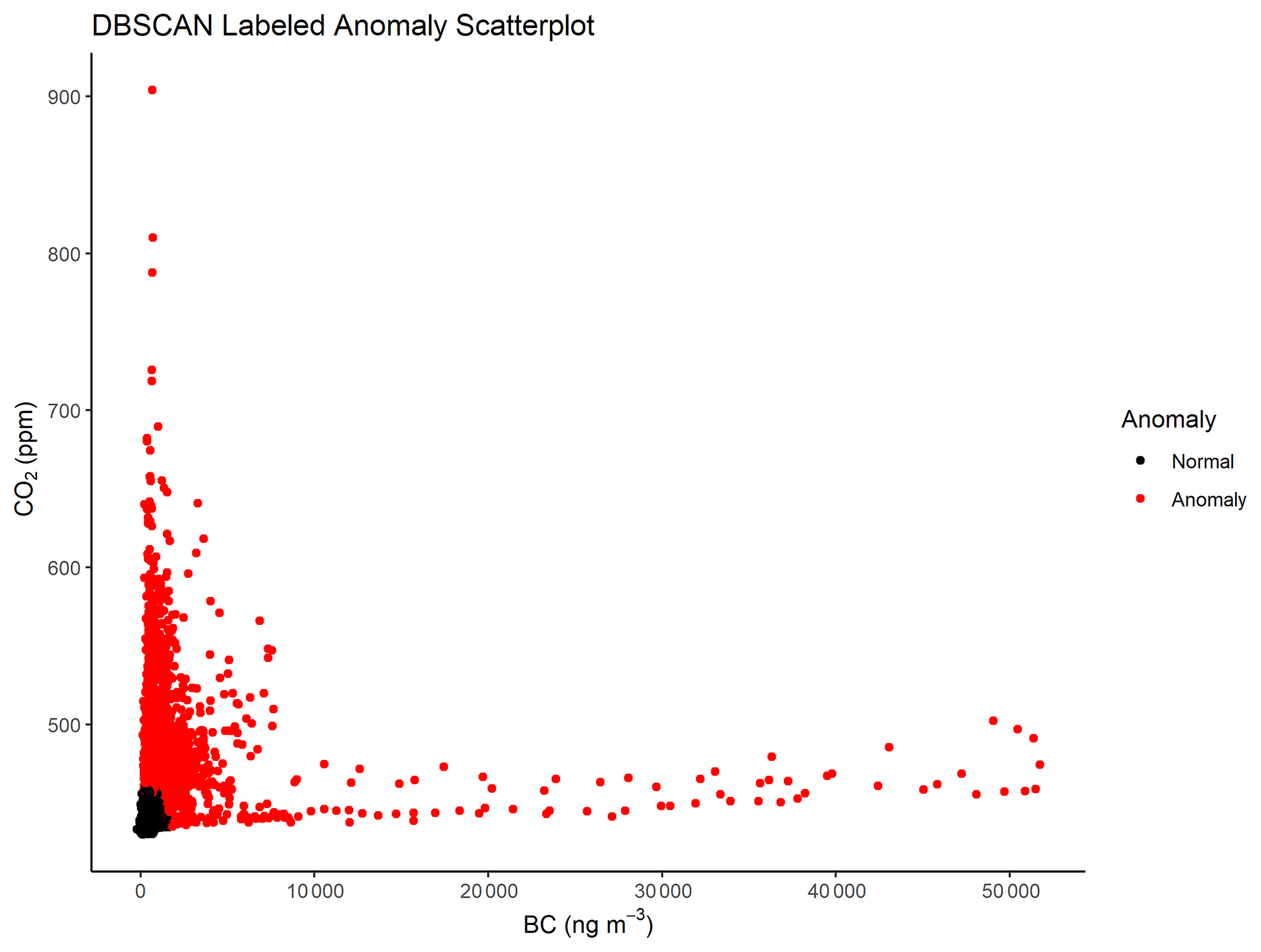
Figure 2Daily scatterplot example of DBSCAN labeled anomalies (red) for CO2 against BC. Points labeled as normal (black and clustered near the origin) are approximately two-thirds of the time series realizations in this example.
2.5 Description of other algorithms
To put the performance of the DBSCAN anomaly detection algorithm in context, we compare its labeled anomalies with output from the previously described plume detection technique of Drewnick et al. (2012) (referred to as “Drewnick” moving forward) or base-case 90th-quantile algorithms. These two base-case algorithms, the Quantile-OR (QOR) and the Quantile-AND (QAND) algorithms, flag points as anomalous based on criteria centered around the 90th quantile of pollutant distributions. In the QOR case, points are flagged as anomalous if any one pollutant measurement (BC, CO2, NOx, or UFP) is above the 90th quantile for the given daily time series (if BCt > 90th BC, CO2,t > 90th CO2, Ox,t > 90th NOx, or UFPt > 90th UFP). In the QAND case, points are flagged as anomalous if all pollutant measurements are greater than their respective 90th quantiles (if BCt > 90th BC, CO2,t > 90th CO2, NOx,t > 90th NOx, and UFPt > 90th UFP). We run these algorithms, along with the Drewnick algorithm, on all daily time series to assess performance.
2.6 Using the external validation set to tune parameters and evaluate performance
To determine an appropriate value of fval for use in the DBSCAN algorithm, we perform grid search on values of [0.01, 0.10] in increments of 0.01 and [0.15, 0.50] in increments of 0.05. We do not consider values above 0.5 due to computational cost and poor performance at higher values of fval. We evaluate performance using percentage agreement, defined as
where I(.) is the indicator function that evaluates to 1 if the condition is true and 0 otherwise, Pi is the prediction label at point i, Vi is the validation set label at point i, and N is the total number of points in the validation set. Tuning results indicate that a value of 0.03 is most appropriate for fval, which we use in subsequent analyses. In addition to the fval parameter, we tune the quantile parameter with the external validation set. Quantiles near the 90th return only modest improvements, and thus we analyze the 90th quantile.
To evaluate whether we overfit to this validation set, we perform k-fold cross validation with the number of folds, k, equal to five. We train our models on four out of five folds, tuning the fval parameter such that the model performance agreement is maximized on the testing set. We find that the value of fval that results in superior performance is 0.03, suggesting that our work above generalizes appropriately. The k-fold cross-validation results are given in Table S2.
We also use the same validation set to compare performance across all four algorithms examined in this study. We evaluate the performance of each by calculating the percentage agreement between each algorithm's labels and the validation set labels.
2.7 Interpretation: k-means clustering and PCA
We perform k-means clustering on the extracted anomalies using the kmeans function available in R's base package (R Core Team, 2022). We set the number of centers (clusters) to 3 and choose 200 iterations with different random starts to ensure the derived result was robust to utilized starting values. We assign cluster labels based on the cluster means to ensure consistency in label assignment. We use prcomp available in the R base package to calculate principal component loadings and scores for visualization (R Core Team, 2022). We use the R packages scattermore (Kratochvil, 2022) and tidyverse (Tidyverse, 2022) for the visualization itself. We perform Varimax rotation using R package psych (Revelle, 2022) to compare to results from a previously published study (Larson et al., 2017).
We create boxplots of assigned roadway trucking variables to probe potential meanings of clustered anomalies. We extract roadway trucking variables from the Texas Department of Transportation's (TxDOT) roadway inventory (Texas Department of Transportation, 2021) with processing performed using R package sf (Pebesma, 2018a). We average records along the same road segment with weights equivalent to the distance between fields in the shapefile FROM_DFO and TO_DFO, which are distance measures representing starting and ending points for those records in the shapefile. Extracted roadway variables from the shapefile include annual average daily traffic counts (AADT), truck AADT percentage (TRUCK_AADT_PCT), and the number of all trucks in AADT (AADT_TRUCKS).
2.8 Census tract assignment
To determine differences in anomaly frequency between census tracts, we assign points (Pebesma, 2018a) to census tracts using tract boundaries stored in a shapefile used in a previously published analysis of the same campaign data (Miller et al., 2020; Actkinson et al., 2021). We count anomalies of a given cluster assignment and divide by the total recorded measurements in each polygon. Because each census tract was sampled at different hours from one another and because the objective of the analysis was to compare census tracts, we implement a rescaling procedure described in detail in Sect. S1. As part of that procedure, we restrict the comparisons to 19 of the 35 census tracts to measurements taken between 08:00 and 16:00 LT (local time) and measurements taken on weekdays. To account for different polygons containing differing numbers of measurements, we divide the total amount of rescaled anomaly types by the total number of measurements made in the census tract, deriving a probability of encountering the specified anomaly type during the campaign in the restricted time interval described above. This probability represents the chance of detection of a given anomaly during the campaign study period. Sect. S2 describes a bootstrapping procedure used to estimate errors associated with these probabilities, which are provided in Tables S3, S4, and S5.
3.1 External validation
We run all four algorithms – Drewnick, QOR, QAND, and DBSCAN – on the Houston mobile monitoring campaign data. To differentiate performance, we compare each algorithm's labeled anomalies with the anomalies of the validation set on the same subset of days, which are considered the ground truth. We observed the algorithm to capture clean conditions as well; the DBSCAN algorithm labeled 848 multivariate realizations with all pollutants lower than their respective fifth quantiles as noise or just 0.07 % of the total number of labeled anomalies.
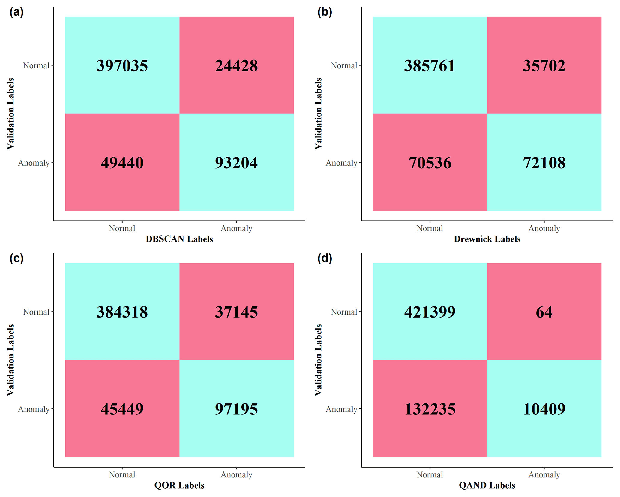
Figure 3Confusion matrices corresponding to the performance of (a) DBSCAN, (b) Drewnick, (c) QOR, and (d) QAND. Overall agreement between each algorithm and the validation set was (a) 86.9 %, (b) 85.5 %, (c) 81.8 %, and (d) 77.0 %, respectively. For example, DBSCAN and the validation efforts both label 397 035 points as normal and 93 204 as anomalous. DBSCAN labels 49 440 points as normal when the validation efforts label them as anomalous; conversely, DBSCAN labels 24 428 points as anomalous when the validation efforts label them as normal.
Of the four algorithms, DBSCAN had the best performance, with its labels exhibiting 86.9 % agreement with the validation set's labels. The QOR, QAND, and Drewnick algorithms exhibit 85.5 %, 77.0 %, and 81.8 % agreement, respectively. For context, an algorithm that simply labeled all points as normal would generate 74.7 % agreement with the validation set. Because this baseline agreement is so high, we create confusion matrices to probe sources of agreement and disagreement between each algorithm's predicted anomalies and the validation set labeled anomalies and display them in Fig. 3. Confusion matrices compare how an algorithm categorizes points with the points' true categories. In our work, confusion matrices tabulate the number of points that a given algorithm labels as normal or as an anomaly that are correspondingly labeled as normal or as an anomaly in the validation set.
Figure 3 illustrates that even though the DBSCAN algorithm exhibits greater overall agreement with the validation set, it predicts anomalies less successfully compared to the QOR algorithm. However, the DBSCAN algorithm outperforms the QOR algorithm in its ability to not predict normal points as anomalous. This suggest that the QOR algorithm captures the most anomalies but is a coarse approach to doing so; the DBSCAN algorithm captures fewer anomalies but is less likely to predict something as anomalous when it is not. Table S6 contains counts of instances in which one algorithm made a mistake of a given type when the other did not. Table S6 provides further evidence that the DBSCAN algorithm is inferior in its ability to label anomalous points compared to the QOR algorithm, while the QOR algorithm is inferior in its ability to not label normal points as anomalous. For the purposes of further analysis, we focus our attention on DBSCAN-derived anomalies, bringing in QOR-derived anomalies periodically for comparison. We choose to focus on results from DBSCAN as the approach is more conservative; it does not result in as many false positives as the QOR algorithm and provides confidence that what is being analyzed is an anomaly. The QAND and Drewnick algorithms do not offer superior performance over the DBSCAN and QOR algorithms, and we do not consider them for further analysis.
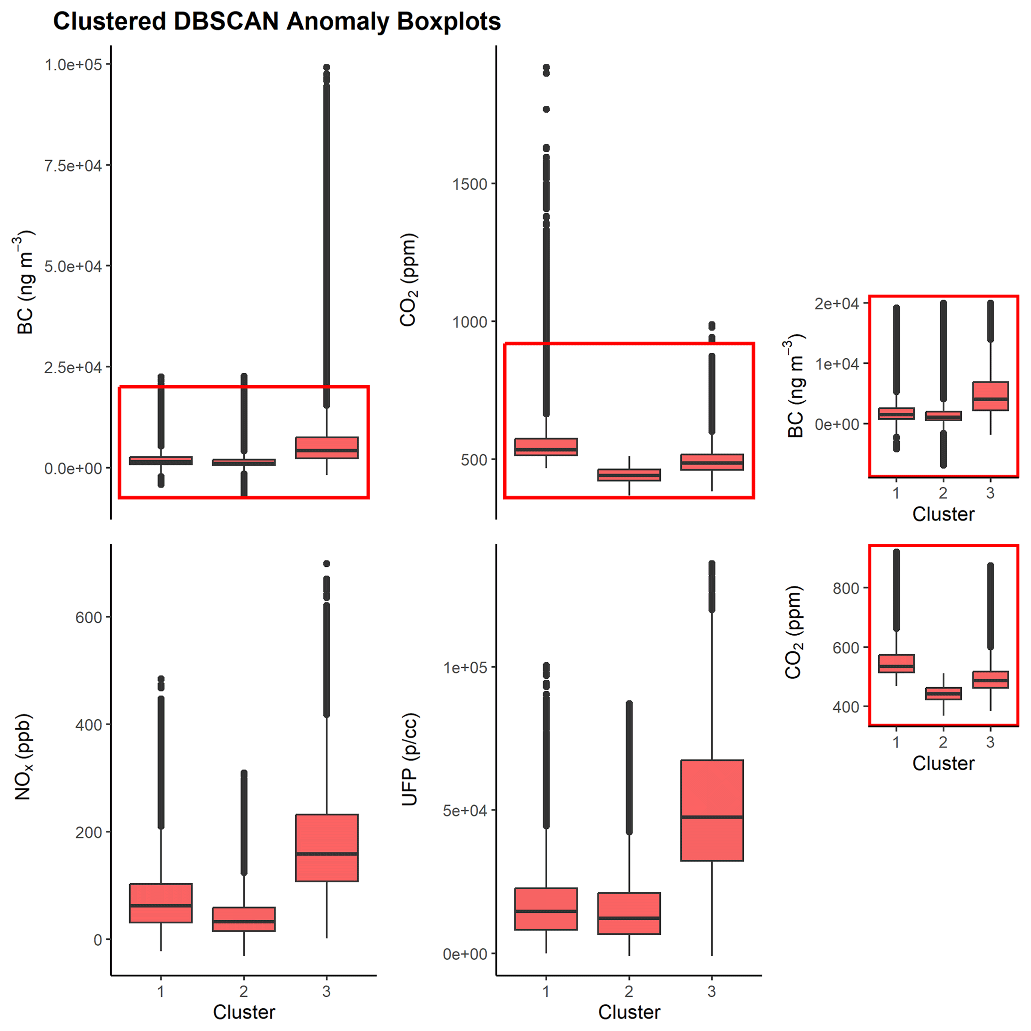
Figure 4Boxplots of clustered DBSCAN anomalies by cluster label. Red rectangles correspond to insets of CO2 and BC that are displayed on the right side of the plot.
3.2 The k-means clustering and PCA
We cluster detected anomalies using R function kmeans, which consistently yields one cluster rich in CO2 concentrations (“CO2 cluster”), another cluster that contains lower (but still higher than their non-anomaly counterparts) concentrations of all four pollutants for both QOR- and DBSCAN-derived anomalies (“transition cluster”), and a third cluster rich in BC NOx/UFP (“BC UFP cluster”) concentrations. Table 1 and Figs. 4 and S5 contain statistics describing the contents of each cluster. The results are consistent with previously published emissions patterns associated with light and heavy-duty vehicles. Heavy-duty, diesel-powered vehicles emit more BC, NOx, and UFP per kilogram of fuel than light-duty vehicles, often an order of magnitude or more (Dallmann et al., 2012, 2013; Park et al., 2011; Preble et al., 2018). Additionally, loadings from the PCA biplot in Fig. S5 when varimax rotated are consistent in split with those reported in Larson et al. (2017); loadings are sequestered into BC- or UFP-rich and CO2-rich factors, which are attributed to heavy- and light-duty vehicle activity, respectively. These loadings are given in Table S7.
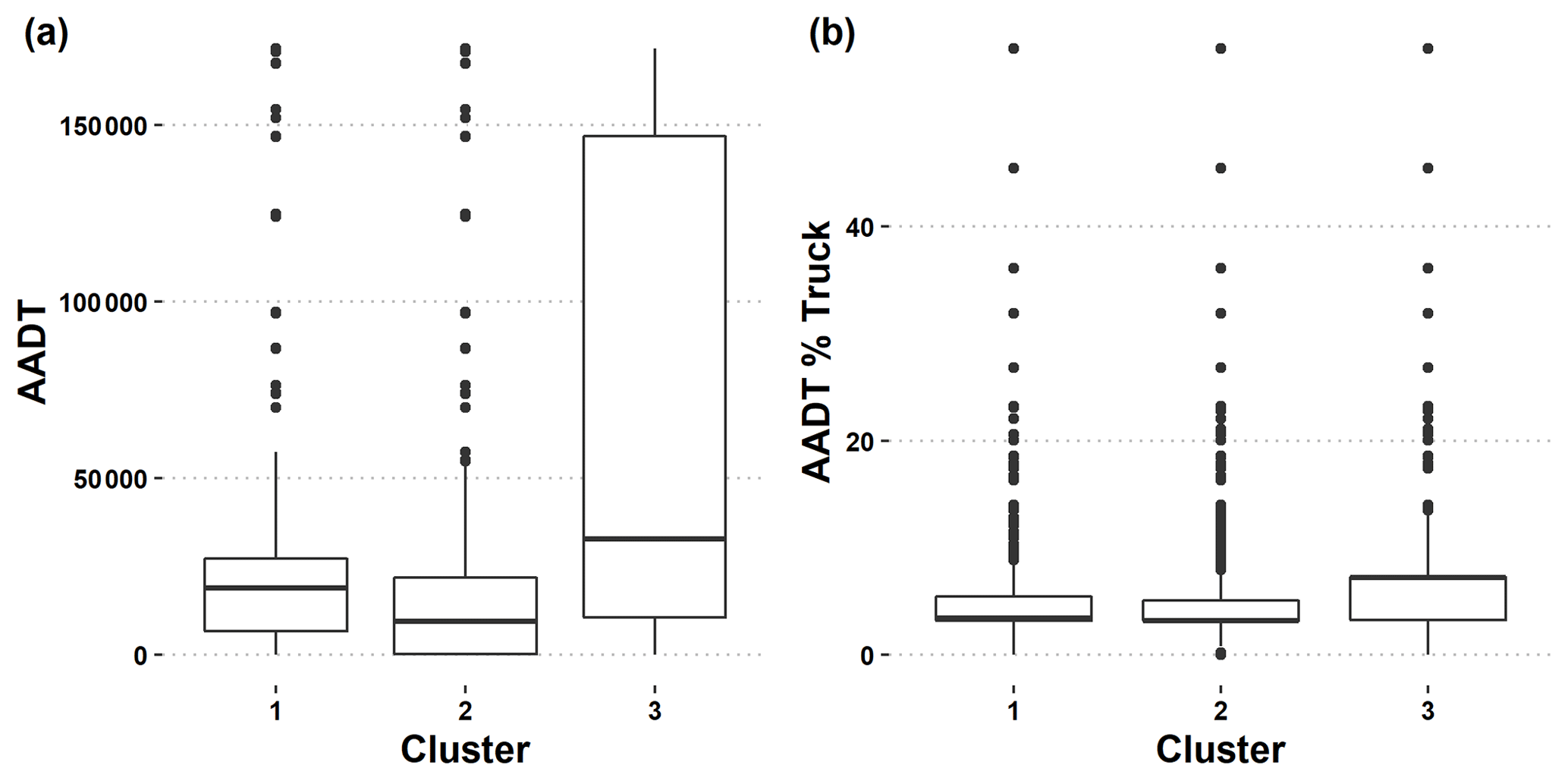
Figure 5Boxplot of traffic attributes corresponding to anomalies in labeled clusters (1 – “CO2 cluster”; 2 – “transition cluster”; 3 – “BC UFP cluster”). (a) Annual average daily traffic (AADT) by cluster label. (b) Percentages of trucks in the annual average daily traffic counts (AADT% Truck).
Table 1DBSCAN and QOR k-means cluster means for the four pollutants considered.
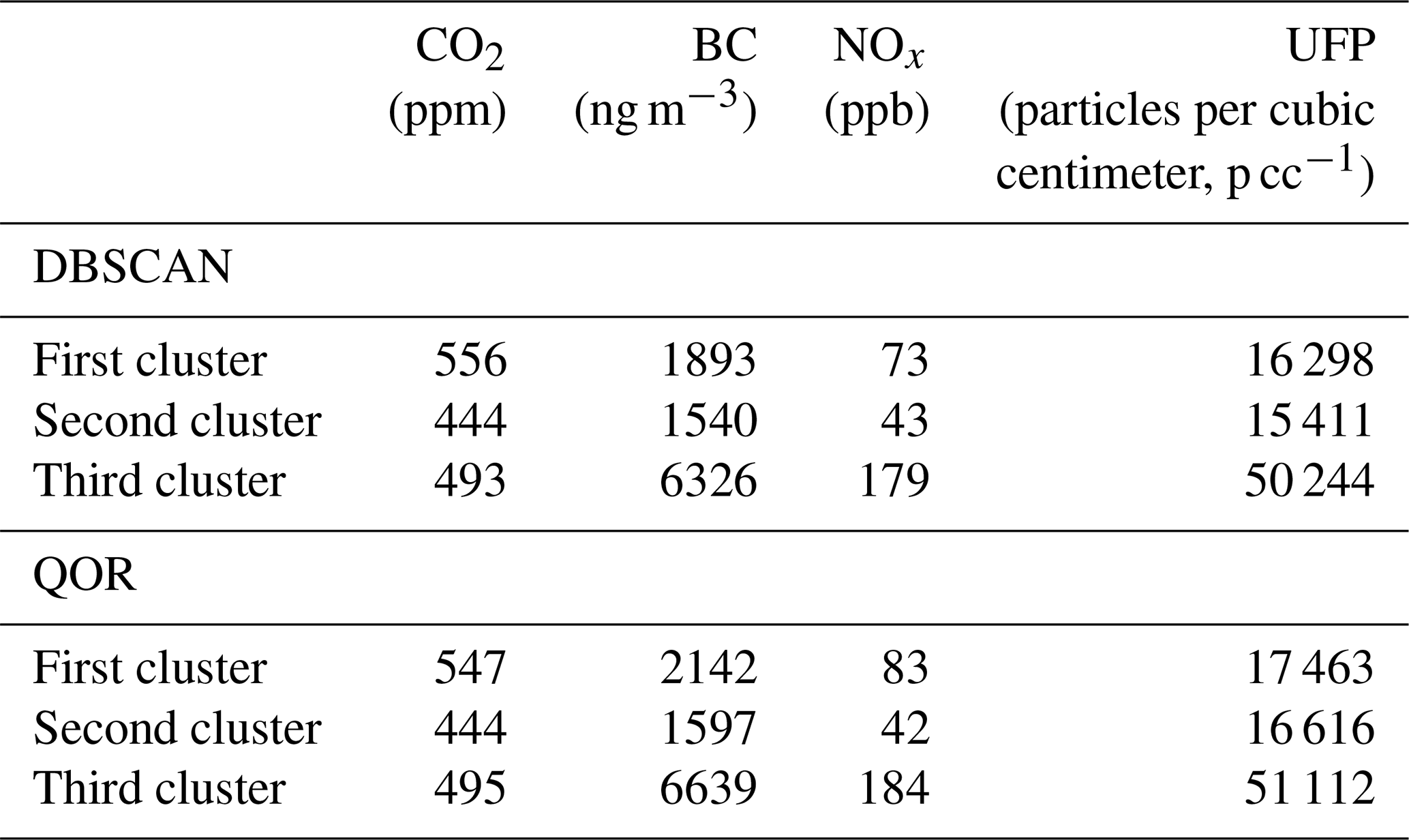
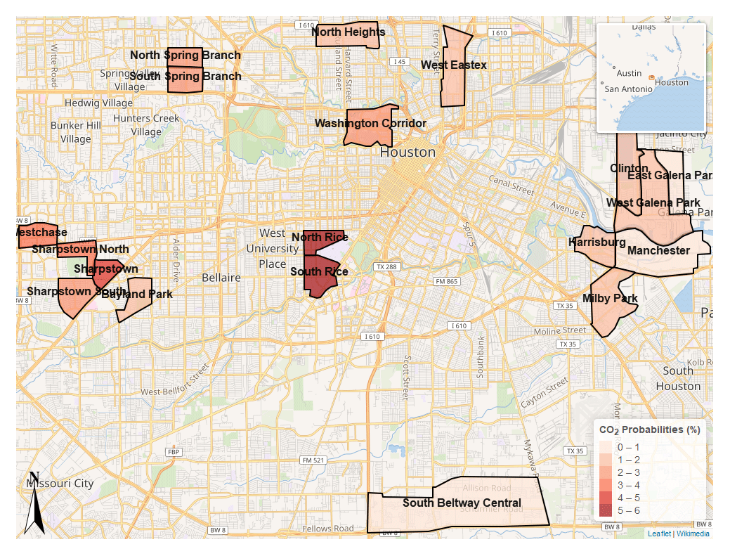
Figure 6Map depicting analyzed census tracts colored (darker indicates larger probability) by their calculated CO2 anomaly detection probabilities (%). Wikimedia, 2021. Distributed under the Creative Commons Attribution-ShareAlike 4.0 license. https://foundation.wikimedia.org/w/index.php?title=Maps_Terms_of_Use#Where_does_the_map_data_come_from.3F (last access: 11 November 2022).
To verify vehicle-related impacts associated with these clusters, we extract traffic variables from the TxDOT roadway inventory and assign these values to our clustered anomalies based on nearest-neighbor assignment between the logged GPS coordinates of each clustered point and the latitude and longitude coordinates of the inventory's features (Texas Department of Transportation, 2021). We plot these assignments in Fig. 5. Figure 5a contains the overall AADT counts. Figure 5b shows percentages of trucks in the estimated annual AADT counts. The high percentage of trucks in AADT in the BC UFP cluster suggests that the cluster is related to trucking activity, while the lower trucking percentage in combination with elevated AADT compared to the transition cluster suggests that the CO2 cluster is capturing light-duty vehicle activity. Results from these boxplots confirm that our clusters are linked to emissions from these different vehicle types.
3.3 Detected anomaly type by census tract
To evaluate spatial differences in these clustered anomaly types across the city of Houston, we tabulate anomaly types for a subset of visited census tracts; details about the census tracts are provided in Table S8. We report rescaled total numbers of detected anomalies of a given cluster type (CO2 cluster for CO2-rich, transition cluster, BC UFP cluster) divided by the total number of measurements made in that census tract. Normalizing by the total number of measurements in this manner yields the probability of encountering the anomaly in the census tract during the study period, which is from 08:00 to 16:00 LT on weekdays. Figure S6 displays bar plots showing DBSCAN anomaly detection type probabilities by census tract, while Figs. 6 and 7 map the census tracts colored by their CO2 and BC UFP anomaly detection type probabilities.

Figure 7Map depicting analyzed census tracts colored (darker indicates larger probability) by their calculated BC UFP anomaly detection probabilities (%). Wikimedia, 2021. Distributed under the Creative Commons Attribution-ShareAlike 4.0 license. https://foundation.wikimedia.org/w/index.php?title=Maps_Terms_of_Use#Where_does_the_map_data_come_from.3F.
The bar plots and maps illustrate stark spatial heterogeneity in anomaly type. With respect to CO2 cluster anomalies, neighborhoods in the western parts of Houston (North Rice, South Rice, Sharpstown) consistently rank higher than neighborhoods in the eastern part of Houston (Milby Park, Clinton, Manchester), with neighborhoods surrounding Rice University ranking the highest. The neighborhoods near the Rice campus consist of busy thoroughfares that are often congested with traffic from light-duty gasoline-powered vehicles, especially around local rush hour (08:00 LT). With regards to the BC UFP clusters, heavily industrialized neighborhoods in the eastern part of Houston near the Houston Ship Channel (Milby Park, West Galena Park, Manchester, Clinton) are ranked the highest, with the Milby Park census tract exhibiting the highest probability of encountering one of these anomaly types (10.6 %) during the study period.
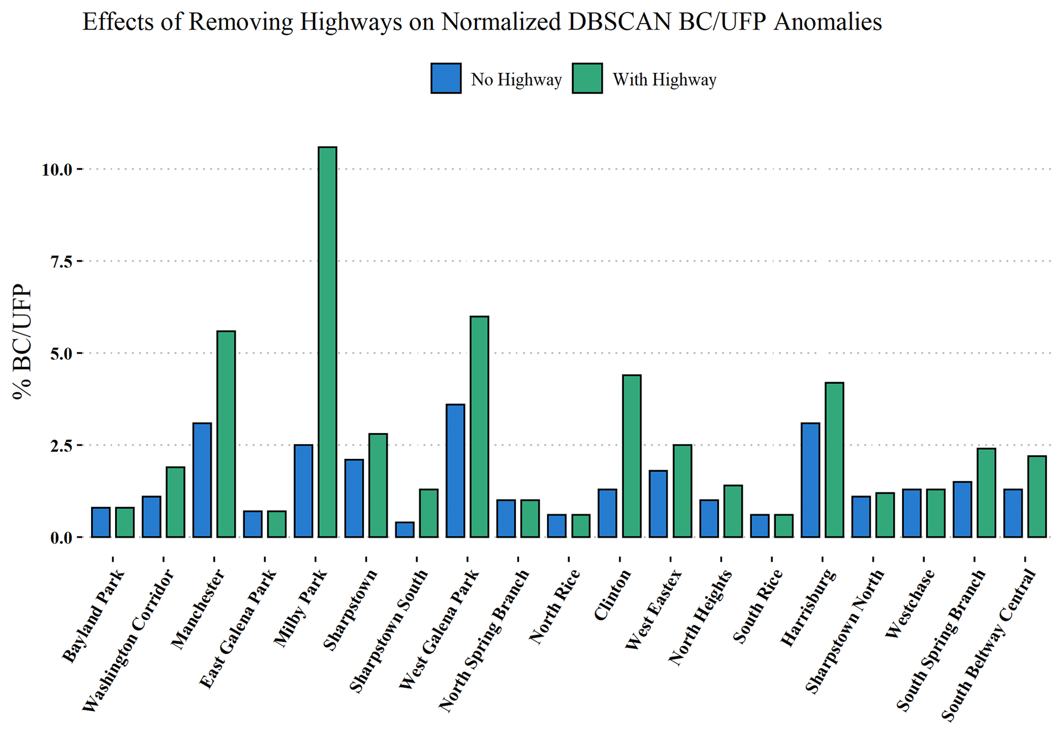
Figure 8Probability of detecting BC UFP anomaly type with highways in the analysis (green, right bar for each census tract) and without highways in the analysis (blue, left bar for each census tract).
Table 2Tabulated anomaly detection probability type (“CO2-rich” is listed as “CO2 %”, “transition” is listed as “transition %”, “BC- UFP-rich” is listed as “BC UFP %”) by census tract. For example, the italicized entries in this table indicate a ∼ 10 × greater chance of encountering a BC/UFP anomaly type in the Manchester census tract compared to the North Rice census tract.

Many of the BC UFP anomaly detections occur on highways; Fig. 8 illustrates the differences in BC UFP anomaly detection probabilities when highways are included and excluded from the analysis (Fig. S7 shows the same information for CO2 anomalies). Even with highways removed from the analysis, neighborhoods in the eastern part of Houston still rank consistently higher than those neighborhoods in the western part of Houston with respect to the frequency of BC UFP anomaly detection. The mapped census tracts show spatial discrepancies between CO2-dominated and BC UFP-dominated areas with respect to probability of anomaly type detection. Table 2 details probabilities of detecting each anomaly type by census tract, underscoring these spatial disparities. For example, the italicized entries in Table 2 indicate a ∼ 10 × greater chance of encountering a BC UFP anomaly type in the Manchester census tract compared to the North Rice census tract. These disparities, and the presented evidence suggesting that the BC UFP anomalies are closely related to heavy-duty vehicles, are consistent with previous modeling studies that show large contributions of heavy-duty vehicles to air pollution in Houston's Ship Channel (HSC) neighborhoods and previous work pointing out elevated heavy-duty vehicle activity in the HSC area (Zhang et al., 2017; Demetillo et al., 2020).
We discuss the successful development of a new approach to detect plumes in mobile monitoring time series using an anomaly detection algorithm based on DBSCAN and use the resulting analysis to derive anomaly frequencies representative of different emission impacts in different Houston neighborhoods. While previous work has implemented DBSCAN in conjunction with deep-learning models to analyze satellite PM2.5 measurements (Lu et al., 2021) or to define microenvironments in air pollution exposure contexts (e.g., home, work, or restaurants) (Do et al., 2021), this is the first study to incorporate DBSCAN in plume detection efforts. The algorithm offers comparable, if not superior, performance to previously published plume detection techniques for mobile monitoring time series and is justified in analyses warranting a conservative approach. In this work, we show how this approach illustrates different emission impacts in census tracts around the city of Houston. Specifically, we show how BC and UFP anomaly frequencies were ≈ 10 × greater in census tracts in the eastern part of Houston near the HSC compared to neighborhoods in the western part of Houston. While it is not definitive that this cluster type represents impacts from heavy-duty vehicles, as there is no observational evidence to connect those observations to those vehicle types directly, anomaly emission patterns are consistent with previously published studies analyzing emissions from light- and heavy-duty vehicles (e.g., Larson et al., 2017, and references therein). Previous studies also have shown the large impacts of trucking on pollution in the HSC area and have raised environmental justice concerns with the burden of pollution from diesel-powered-vehicle activity (Demetillo et al., 2020; Zhang et al., 2017). Results from this work emphasize the need for additional investigation into trucking activity in HSC neighborhoods and, more broadly, illustrate how mapped spatial distributions of these anomalies can be used to inform regulatory activities.
Results from this algorithm could be incorporated into health assessment frameworks. Clustered anomalies could be grouped into source categories to facilitate simple exposure estimates from different sources. Apportioning anomalies to nearby sources and determining their frequencies would be an interesting approach to determining whether some sources are more harmful to health than other sources. Census-tract-weighted probabilities of an anomaly could be employed in random walk simulations of cumulative air pollution exposure, providing a different metric to evaluate related health effects (Tang and Niemeier, 2021). Future work could focus on addressing serial dependency inherent in detected anomalies to develop probability-based exposure estimates and the general development of a framework that relates health outcomes to the frequencies of these detected anomalies.
There are opportunities to improve this algorithm in future work. For example, this algorithm should be evaluated using different external validation methods, such as having an observer sit in the vehicle and note emissions events (for example, driving behind a heavy-duty diesel vehicle), while data are being collected to create the validation set. Additionally, the mobile platform could be co-located with a wide suite of stationary instruments to enable more confidence in source identification. Alternative nearest-neighbor clustering techniques could be explored; local outlier factors could be used to address situations where DBSCAN does not exhibit great performance (Tan et al., 2019). An ensemble approach utilizing both DBSCAN and other clustering techniques could be investigated for improved performance (Drewnick et al., 2012; Actkinson et al., 2021). Future work also could consider aggregating data on a scale finer than a census tract to address heterogeneity of emissions within a census tract.
A GitHub repository containing code used to generate the work is available here: https://doi.org/10.5281/zenodo.7700290 (Actkinson, 2023a).
Additionally, an R Shiny application containing a graphical user interface to the software is available at the following URL: https://bactkinson.shinyapps.io/plume_detection_with_dbscan/ (Actkinson, 2023c). The DOI for the repository containing code used to generate the Shiny app is available here: https://doi.org/10.5281/zenodo.7700300 (Actkinson, 2023b).
The following R packages were used in the analysis and visualization of results: tidyverse (https://www.tidyverse.org/; Tidyverse, 2022), ggpubr (https://CRAN.R-project.org/package=ggpubr; Kassambara, 2020), caret (https://CRAN.R-project.org/package=caret; Kuhn, 2022), dbscan (https://CRAN.R-project.org/package=dbscan; Hahsler and Piekenbrock, 2022; Hahsler et al., 2019), Leaflet for R (https://CRAN.R-project.org/package=leaflet; Cheng et al., 2022), leafem (https://CRAN.R-project.org/package=leafem; Appelhans, 2021), sf (https://CRAN.R-project.org/package=sf; Pebesma, 2018b, a), Mapview (https://github.com/r-spatial/mapview; Appelhans et al., 2022), scattermore (https://CRAN.R-project.org/package=scattermore; Kratochvil, 2022), psych (https://CRAN.R-project.org/package=psych; Revelle, 2022), base (R Core Team, 2022), and data.table (https://CRAN.R-project.org/package=data.table; Dowle and Srinivasan, 2021).
Validation data sets used in this work are available at the following Zenodo repository: https://doi.org/10.5281/zenodo.6473859 (Actkinson and Griffin, 2022).
The Texas Department of Transportation Road Inventory is available for download here: https://www.txdot.gov/data-maps/roadway-inventory.html (Texas Department of Transportation, 2021).
The 2018 TIGER/Line Shapefile, created and maintained by the United States Census Bureau, is available for download here: https://catalog.data.gov/dataset/tiger-line-shapefile-2018-county-harris-county-tx-all-roads-county-based-shapefile (U.S. Census Bureau, 2018).
The supplement related to this article is available online at: https://doi.org/10.5194/amt-16-3547-2023-supplement.
BA conceived, wrote, and analyzed the plume detection algorithm with helpful insight from RJG. BA wrote the manuscript. RJG provided helpful edits and suggestions.
The contact author has declared that none of the authors has any competing interests.
Publisher's note: Copernicus Publications remains neutral with regard to jurisdictional claims in published maps and institutional affiliations.
The authors gratefully acknowledge the support of the National Institute of Environmental Health Sciences (NIEHS, grant no. R01ES028819-01). Additionally, we appreciate the support of Environmental Defense Fund for the collection and provision of the mobile data used to develop this algorithm. Finally, we acknowledge Katherine Ensor and Daniel Cohan for useful suggestions and input.
This research has been supported by the National Institute of Environmental Health Sciences (grant no. R01ES028819-01).
This paper was edited by John Sullivan and reviewed by two anonymous referees.
Actkinson, B.: bactkinson/Anomaly_Analysis: AMT Preprint Submission (AMT), Zenodo [code], https://doi.org/10.5281/zenodo.7700290, 2023a.
Actkinson, B.: bactkinson/Plume_Detection_with_DBSCAN: Plume Detection with DBSCAN – R Shiny App (AMT), Zenodo [code], https://doi.org/10.5281/zenodo.7700300, 2023b.
Actkinson, B.: DBSCAN Plume Detection Tool, shinyapps.io [code], https://bactkinson.shinyapps.io/plume_detection_with_dbscan/ (last access: 6 March 2023), 2023c.
Actkinson, B. and Griffin, R.: Datasets used in Detecting Plumes in Mobile Air Quality Monitoring Time Series with Density-based Spatial Clustering of Applications with Noise v01, Zenodo [data set], https://doi.org/10.5281/zenodo.6473859, 2022.
Actkinson, B., Ensor, K., and Griffin, R. J.: SIBaR: a new method for background quantification and removal from mobile air pollution measurements, Atmos. Meas. Tech., 14, 5809–5821, https://doi.org/10.5194/amt-14-5809-2021, 2021.
Appelhans, T.: leafem: “leaflet” Extensions for “mapview”, CRAN [code], https://CRAN.R-project.org/package=leafem (last access: 11 November 2022), 2021.
Appelhans, T., Detsch, F., Reudenbach, C., and Woellauer, S.: mapview: Interactive Viewing of Spatial Data in R, GitHub [code], https://github.com/r-spatial/mapview (last access: 11 November 2022), 2022.
Cheng, J., Karambelkar, B., and Xie, Y.: leaflet: Create Interactive Web Maps with the JavaScript “Leaflet” Library, CRAN [code], https://CRAN.R-project.org/package=leaflet (last access: 11 November 2022), 2022.
Dallmann, T. R., DeMartini, S. J., Kirchstetter, T. W., Herndon, S. C., Onasch, T. B., Wood, E. C., and Harley, R. A.: On-road measurement of gas and particle phase pollutant emission factors for individual heavy-duty diesel trucks, Environ. Sci. Technol., 46, 8511–8518, https://doi.org/10.1021/es301936c, 2012.
Dallmann, T. R., Kirchstetter, T. W., DeMartini, S. J., and Harley, R. A.: Quantifying on-road emissions from gasoline-powered motor vehicles: Accounting for the presence of medium- and heavy-duty diesel trucks, Environ. Sci. Technol., 47, 13873–13881, https://doi.org/10.1021/es402875u, 2013.
Demetillo, M. A. G., Navarro, A., Knowles, K. K., Fields, K. P., Geddes, J. A., Nowlan, C. R., Janz, S. J., Judd, L. M., Al-Saadi, J., Sun, K., McDonald, B. C., Diskin, G. S., and Pusede, S. E.: Observing nitrogen dioxide air pollution inequality using high-spatial-resolution remote sensing measurements in Houston, Texas, Environ. Sci. Technol., 54, 9882–9895, https://doi.org/10.1021/acs.est.0c01864, 2020.
Do, K., Yu, H., Velasquez, J., Grell-Brisk, M., Smith, H., and Ivey, C. E.: A data-driven approach for characterizing community scale air pollution exposure disparities in inland Southern California, J. Aerosol Sci., 152, 105704, https://doi.org/10.1016/j.jaerosci.2020.105704, 2021.
Dowle, M. and Srinivasan, A.: data.table: Extension of “Data.Frame”, CRAN [code], https://CRAN.R-project.org/package=data.table (last access: 11 November 2022), 2021.
Drewnick, F., Böttger, T., von der Weiden-Reinmüller, S.-L., Zorn, S. R., Klimach, T., Schneider, J., and Borrmann, S.: Design of a mobile aerosol research laboratory and data processing tools for effective stationary and mobile field measurements, Atmos. Meas. Tech., 5, 1443–1457, https://doi.org/10.5194/amt-5-1443-2012, 2012.
Ester, M., Kriegel, H.-P., and Xu, X.: A density-based algorithm for discovering clusters in large spatial databases with noise, in: KDD'96: Proceedings of the Second International Conference on Knowledge Discovery and Data Mining, Portland, Oregon, USA, 2–4 August 1996, AAAI Press, 226–231, https://dl.acm.org/doi/10.5555/3001460.3001507, 1996.
Hagler, G. S. W., Lin, M.-Y., Khlystov, A., Baldauf, R. W., Isakov, V., Faircloth, J., and Jackson, L. E.: Field investigation of roadside vegetative and structural barrier impact on near-road ultrafine particle concentrations under a variety of wind conditions, Sci. Total Environ., 419, 7–15, https://doi.org/10.1016/j.scitotenv.2011.12.002, 2012.
Hahsler, M. and Piekenbrock, M.: dbscan: Density-Based Spatial Clustering of Applications with Noise (DBSCAN) and Related Algorithms, CRAN [code], https://CRAN.R-project.org/package=dbscan (last access: 11 November 2022), 2022.
Hahsler, M., Piekenbrock, M., and Doran, D. Dbscan: Fast density-based clustering with R, J. Stat. Softw., 91, 1–30, https://doi.org/10.18637/jss.v091.i01, 2019.
Kassambara, A.: Ggpubr: “ggplot2” Based Publication Ready Plots, CRAN [code], https://CRAN.R-project.org/package=ggpubr (last access: 11 November 2022), 2020.
Kratochvil, M.: Scattermore: Scatterplots with More Points, CRAN [code], https://CRAN.R-project.org/package=scattermore (last access: 11 November 2022), 2022.
Kuhn, M.: caret: Classification and Regression Training, CRAN [code], https://CRAN.R-project.org/package=caret (last access: 11 November 2022), 2022.
Larson, T., Gould, T., Riley, E. A., Austin, E., Fintzi, J., Sheppard, L., Yost, M., and Simpson, C.: Ambient air quality measurements from a continuously moving mobile platform: Estimation of area-wide, fuel-based, mobile source emission factors using absolute principal component scores, Atmos. Environ., 152, 201–211, https://doi.org/10.1016/j.atmosenv.2016.12.037, 2017.
Lu, X., Wang, J., Yan, Y., Zhou, L., and Ma, W.: Estimating hourly PM2.5 concentrations using Himawari-8 AOD and a DBSCAN-modified deep learning model over the YRDUA, China, Atmos. Poll. Res., 12, 183–192, https://doi.org/10.1016/j.apr.2020.10.020, 2021.
Messier, K. P., Chambliss, S. E., Gani, S., Alvarez, R., Brauer, M., Choi, J. J., Hamburg, S. P., Kerckhoffs, J., LaFranchi, B., Lunden, M. M., Marshall, J. D., Portier, C. J., Roy, A., Szpiro, A. A., Vermeulen, R. C. H., and Apte, J. S.: Mapping air pollution with Google Street View cars: Efficient approaches with mobile monitoring and land use regression, Environ. Sci. Technol., 52, 12563–12572, https://doi.org/10.1021/acs.est.8b03395, 2018.
Miller, D. J., Actkinson, B., Padilla, L., Griffin, R. J., Moore, K., Lewis, P. G. T., Gardner-Frolick, R., Craft, E., Portier, C. J., Hamburg, S. P., and Alvarez, R. A.: Characterizing elevated urban air pollutant spatial patterns with mobile monitoring in Houston, Texas, Environ. Sci. Technol., 54, 2133–2142, https://doi.org/10.1021/acs.est.9b05523, 2020.
Park, S. S., Kozawa, K., Fruin, S., Mara, S., Hsu, Y.-K., Jakober, C., Winer, A., and Herner, J.: Emission factors for high-emitting vehicles based on on-road measurements of individual vehicle exhaust with a mobile measurement platform, J. Air Waste Manage. Assoc., 61, 1046–1056, https://doi.org/10.1080/10473289.2011.595981, 2011.
Pebesma, E.: Simple Features for R: Standardized Support for Spatial Vector Data, R J., 10, 439–446, https://doi.org/10.32614/RJ-2018-009, 2018a.
Pebesma, E.: sf: Simple Features for R, CRAN [code], https://CRAN.R-project.org/package=sf (last access: 11 November 2022), 2018b.
Preble, C. V., Cados, T. E., Harley, R. A., and Kirchstetter, T. W.: In-use performance and durability of particle filters on heavy-duty diesel trucks, Environ. Sci. Technol., 52, 11913–11921, https://doi.org/10.1021/acs.est.8b02977, 2018.
Qi, M. and Hankey, S.: Using street view imagery to predict street-level particulate air pollution, Environ. Sci. Technol., 55, 2695–2704, https://doi.org/10.1021/acs.est.0c05572, 2021.
R Core Team: R: A language and environment for statistical Computing, R Foundation for Statistical Computing, Vienna, Austria, https://www.R-project.org/, last access: 31 March 2022.
Revelle, W.: psych: Procedures for Personality and Pscyhological Research, CRAN [code], https://CRAN.R-project.org/package=psych (last access: 11 November 2022), 2022.
Shah, R. U., Robinson, E. S., Gu, P., Robinson, A. L., Apte, J. S., and Presto, A. A.: High-spatial-resolution mapping and source apportionment of aerosol composition in Oakland, California, using mobile aerosol mass spectrometry, Atmos. Chem. Phys., 18, 16325–16344, https://doi.org/10.5194/acp-18-16325-2018, 2018.
Tan, P.-N., Steinbach, M., Karpatne, A., and Kumar, V.: Introduction to Data Mining, Pearson, ISBN 0133128903, 2019.
Tang, M. and Niemeier, D. A.: Using big data techniques to better understand high-resolution cumulative exposure assessment of traffic-related air pollution, ACS EST Eng., 1, 436–445, https://doi.org/10.1021/acsestengg.0c00167, 2021.
Tidyverse: https://www.tidyverse.org/, last access: 31 March 2022.
Texas Department of Transportation: Roadway Inventory, Texas Department of Transportation [data set], https://www.txdot.gov/data-maps/roadway-inventory.html (last access: 11 November 2022), 2021.
U.S. Census Bureau: TIGER/Line Shapefile, 2018, county, Harris County, TX, All Roads County-based Shapefile, U.S. Census Bureau [data set], https://catalog.data.gov/dataset/tiger-line-shapefile-2018-county-harris-county-tx-all-roads-county-based-shapefile (last access: 11 November 2022), 2018.
Zhang, X., Craft, E., and Zhang, K.: Characterizing spatial variability of air pollution from vehicle traffic around the Houston Ship Channel area, Atmos. Environ., 161, 167–175, https://doi.org/10.1016/j.atmosenv.2017.04.032, 2017.