A new accurate low-cost instrument for fast synchronized spatial measurements of light spectra

We developed a cost-effective Fast-Response Optical Spectroscopy Time-synchronized instrument (FROST). FROST can measure 18 light spectra in 18 wavebands ranging from 400 to 950 nm with a 20 nm full-width half-maximum bandwidth. The FROST 10 Hz measurement frequency is time-synchronized by a global navigation satellite system (GNSS) timing pulse, and therefore multiple instruments can be deployed to measure spatial variation in solar radiation in perfect synchronization. We show that FROST is capable of measuring global horizontal irradiance (GHI) despite its limited spectral range.

It is very capable of measuring photosynthetic active radiation (PAR) because 11 of its 18 wavebands are situated within the 400-to-700 nm range. A digital filter can be applied to these 11 wavebands to derive the photosynthetic photon flux density (PPFD) and retain information on the spectral composition of PAR.

The 940 nm waveband can be used to derive information about atmospheric moisture.

We showed that the silicon sensor has undetectable zero offsets for solar irradiance settings and that the temperature dependency as tested in an oven between 15 and 46 ^∘C appears very low (−250 ppm K⁻¹). For solar irradiance applications, the main uncertainty is caused by our polytetrafluoroethylene (PTFE) diffuser (Teflon), a common type of diffuser material for cosine-corrected spectral measurements. The oven experiments showed a significant jump in PTFE transmission of 2 % when increasing its temperature beyond 21 ^∘C.

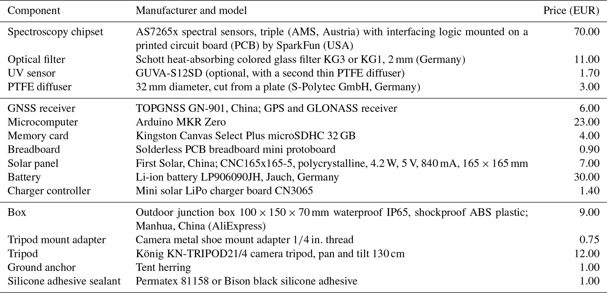
The FROST total cost (< EUR 200) is much lower than that of current field spectroradiometers, PAR sensors, or pyranometers, and includes a mounting tripod, solar power supply, data logger and GNSS, and waterproof housing. FROST is a fully standalone measurement solution. It can be deployed anywhere with its own power supply and can be installed in vertical in-canopy profiles as well. This low cost makes it feasible to study spatial variation in solar irradiance using large-grid high-density sensor setups or to use FROST to replace existing PAR sensors for detailed spectral information.

1 Introduction

Understanding solar irradiance and its interaction with clouds and vegetation is of utmost importance in unraveling the complexity of feedback systems that determine our weather and climate. Cloud-shading dynamics of irradiance are highly dynamic (Lohmann, 2018), and cloud-resolving models (CRMs) are unable to resolve short time intervals and small spatial scales. At grid scales below 1 km, 3-D radiative transfer models can greatly improve the 3-D surface and atmosphere heating rates in atmospheric models (Calahan et al., 2005; Jakub and Mayer, 2015). A good example is the complexity of the radiative effects of shallow cumulus clouds and their interactions with a vegetated surface. Traditional 1-D radiation models produce unrealistic surface radiation fields, but Veerman et al. (2020) showed that a 3-D radiation transfer model could greatly improve the coupling mechanisms between clouds and the land surface. The small circulations, turbulence, and combined cloud microphysics in convective boundary layers are all highly non-linear and complex. CRMs are crucial for improving weather forecasting models and for the energy meteorology sector. Kreuwel et al. (2020) showed that solar-powered grid loading is highly dynamic and especially so for smaller household photovoltaic (PV) systems, leading to grid overload challenges at very short time intervals of seconds. High-quality observations, both in high resolutions spatially and with a high temporal resolution, are required to test such models, but so far observations are lacking (Guichard and Couvreux, 2017).

Yordanov et al. (2013) showed that cloud enhancements can significantly increase solar irradiance levels (> 1.5 times), which result in peak irradiance levels well exceeding extraterrestrial levels even at high altitudes and latitudes (Yordanov, 2015). They used fast-response silicon sensors, and their highest detected irradiance bursts lasted about 1 s, which led them to believe that the required light sensor response time should be at least 0.15 s, much faster than traditional thermopile pyranometers with a response time of several seconds. The slow response time of those thermopile sensors is related to the thermal mass of the thermopile sensor. Semiconductor light sensors respond faster because photons directly mobilize electrons that can be measured directly. The downside of semiconductor light sensors is their limited and non-flat spectral response and temperature sensitivity. Thermopile-based pyranometers are also expensive as compared to a silicon-based solution, which limits their large-scale use in meteorological measurement networks. Martinez et al. (2009) showed that a factor-of-10 reduction in pyranometer costs as compared to a thermopile sensor is possible with the use of a silicon photodiode; however their spectral response is limited (400 to 750 nm) and it has non-flat spectral response. A major solar spectral change occurs in the infrared due to water absorptions bands, which leads to an overestimation for clear-sky conditions and an underestimation for overcast skies when calibrated for average weather conditions.

The spectral-response limitations of the photodiode used by Martinez et al. (2009) can be improved with a wider-spectral-response silicon-type pyranometer such as applied in the LI-COR LI-200SZ as demonstrated by Michalsky et al. (1991). They compared the LI-COR LI-200SZ with a thermopile pyranometer (Kipp & Zonen CM 11). The CM 11 has a flat spectral response (300 to 2500 nm), whereas the LI-COR LI-200SZ exhibits a very non-linear and limited spectral response starting at 400 nm, increasing 5-fold in sensitivity towards its peak at around 1000 nm, and then sharply dropping off to zero at 1100 nm (Alados-Arboleda et al., 1995). Their main uncertainty is related to the temperature dependence of silicon sensors. After a temperature correction, these performed similarly to thermopile pyranometers (11.4 W m⁻² RMSEs) under clear- and cloudy-sky conditions. This is surprisingly accurate because LI-COR calibrates their pyranometer against a reference thermopile pyranometer, and therefore a change in the solar spectrum may affect its accuracy. Michalsky et al. (1991) argued that the clear- or cloudy-sky global horizontal irradiance (GHI) spectra are similar because of clouds mixing the direct and blue skylight. This, however, is contradicted by a recent study by Durand et al. (2021), where they investigated the spectral differences between clear and overcast skies. They showed that clouds, in relative terms, enrich GHI spectra in wavelengths < 465 nm and deplete them in wavelengths > 465 nm. This may well explain why the LI-COR sensor performed so well because its main sensitivity is in wavelengths > 465 nm, thus indirectly correcting for the reduced infrared in the major water absorption bands beyond its spectral range.

Optoelectronics are evolving rapidly, and innovations in semiconductor integration with optical components and microprocessors are paving the way for cost-effective spectrometers that can provide even temperature-compensated spectral details about solar radiation. A leading manufacturer in this field is Austria Micro Systems (AMS), which offers various intelligent light-sensing products that are capable of measuring light intensity within multiple optical wavebands. These sensors are mass-produced, resulting in low-cost sensors. Tran and Fukuzawa (2020) tested such a cost-effective 18-band multispectral sensor (AS7265x, AMS) for spectroscopy of fruit (between 400 and 950 nm), and useful information could be derived. Such filter spectroscopy sensors would be very interesting for solar global horizontal irradiance (GHI) measurements. Quantifying the spectral signature of radiation is very relevant, since clouds and air pollution modify the solar light spectrum and light scattering. Additionally, multiple reflections between various ground and water surfaces and clouds will further influence the light spectral composition. This is especially relevant in the photosynthetic active radiation (PAR) wavelengths for vegetation cloud feedbacks, since PAR affects photosynthesis and evapotranspiration (Durand et al., 2021).

Here we present the development of a cost-effective fast-response solar light sensor grid for spatially and temporally high resolution multiple-light-waveband-resolved GHI measurements. The required large number of sensors necessitates cost-effective design optimization.

Additionally, we tested these sensors for meteorological, photosynthesis, and remote sensing applications as well as performance both in the lab and in field experiments.

2 Instrument design and measurement method

The measurement system we developed is depicted in Fig. 1 (Fast-Response Optical Spectroscopy Time-synchronized instrument – FROST) and consists of a silicon light sensor chipset (AMS AS7265x), a global navigation satellite system (GNSS) for time synchronization, a cosine corrector light-diffusing input port, and a microcomputer. See Table 1 for a list of components.

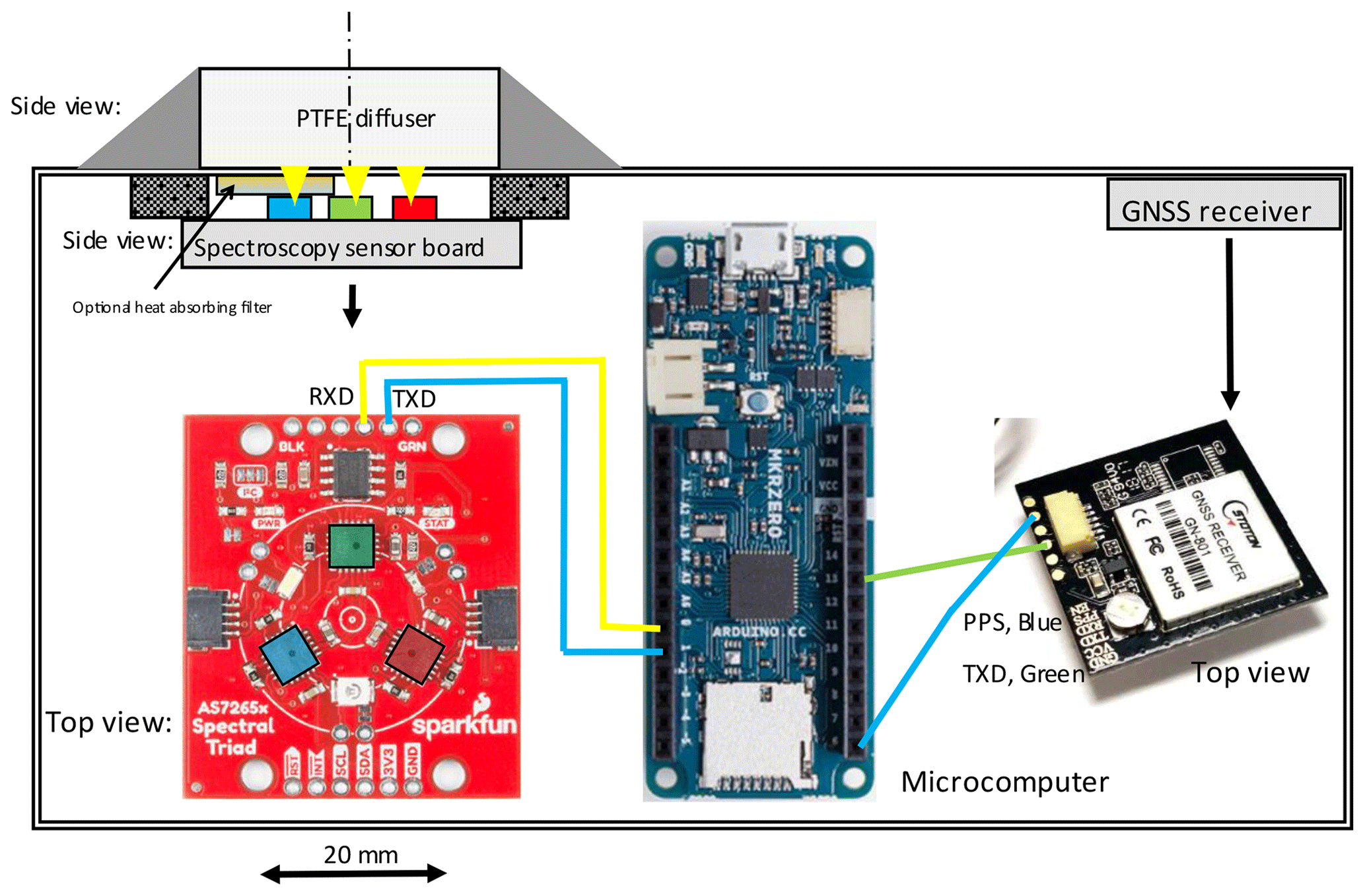
Figure 1 Mechanical layout and wiring diagram of the FROST spectrometer (sensor: 3.2 mm below a Teflon filter with radius of 32 mm). For easy identification we color-coded the three light sensors (blue, green, and red), each measuring six channels. RXD stands for received data and TXD stands for transmitted data.

Table 1 List of components for the waterproof solar-powered spectrometer.

Time-synchronized measurements are achieved using a hardware GNSS receiver timing pulse (PPS) to trigger each measurement, and time-stamped data are processed and collected by a microcomputer board (Fig. 1, Table 1).

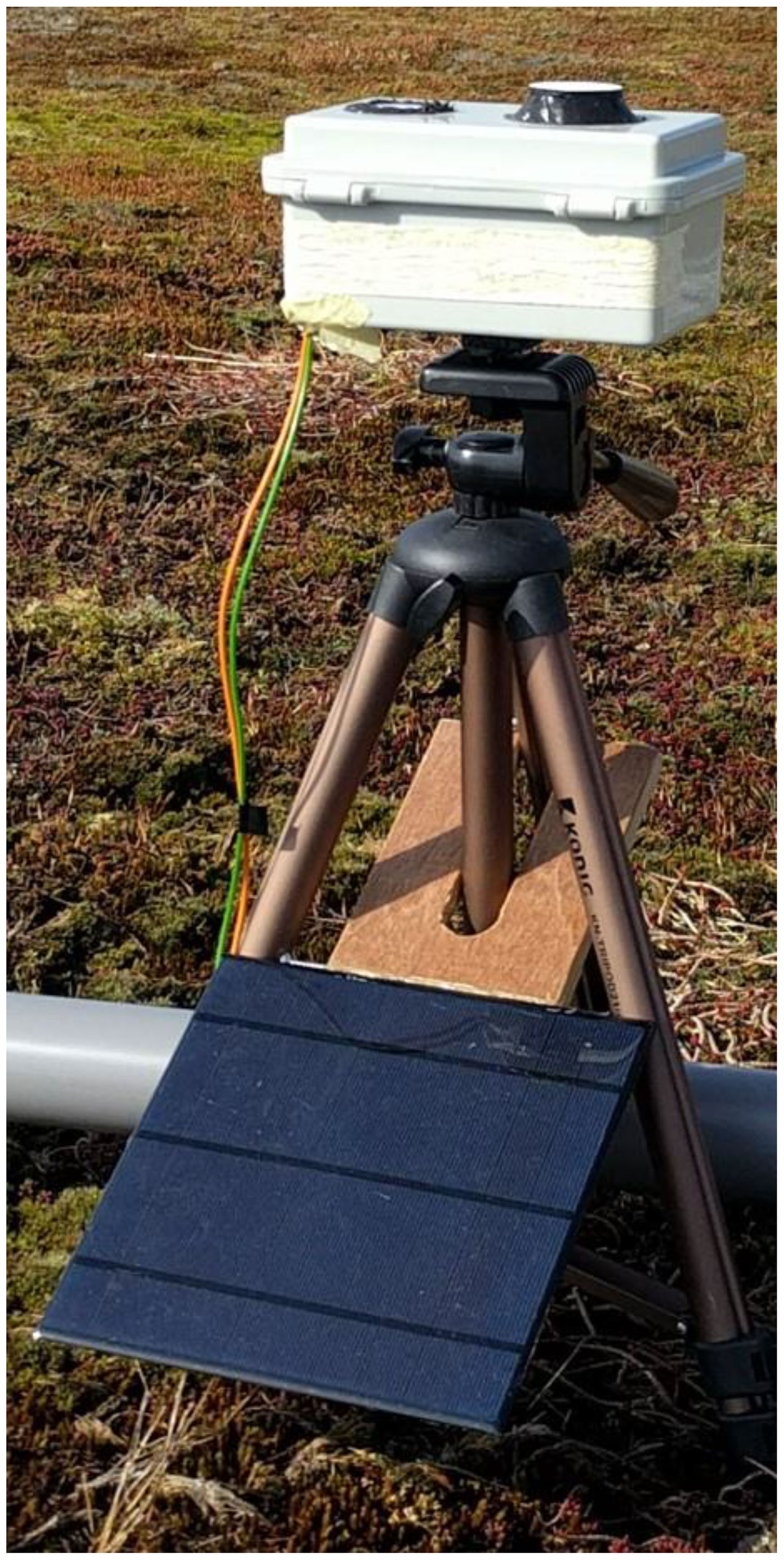
The light sensors are mounted on camera tripods, which makes leveling easy (Fig. 2). A camera metal shoe mount adapter was glued under the polycarbonate housing for fast mounting. For winds > 6 m s⁻¹ it is advised to use tent herrings to fix the tripod to the ground. The power consumption is 0.5 W, and a 6 A h LiPo battery will last for 40 h without sunshine. Battery capacity is reduced at lower temperatures. The 4.2 W polycrystalline solar panel together with a LiPo charge regulator is a reliable power supply solution for continuous operation in the Dutch climate from April–September. The solar panel is glued on a specially shaped wooden frame that slides over the tripod center tube, with the solar panel sides resting against the two outer tripod legs (Fig. 2). It is fixed to the rear leg with a thin metal wire. Hot glue appeared unsuitable for the panels, and it is advised to use epoxy glue.

Figure 2 FROST with solar panel mounted on a camera tripod.

The polytetrafluoroethylene (PTFE) diffuser was glued to the box by roughening the surfaces and using a black silicone adhesive around the diffuser edges.

The correct synchronization of the sensor grid measurements is essential, and several options were considered, such as a network configuration with synchronized triggering at fixed time intervals. Wires in the field were not an option due to logistic challenges, and radio communication is possible but adds to the cost with reduced reliability due to radio interference. As a robust option, a GNSS receiver was chosen that constantly synchronizes its internal time to an international clock standard. Similar timing synchronizations are used for sensors grids in seismic activity monitoring of volcanos where timing is essential to determine seismic propagation and where synchronization accuracy of 50 ns could be achieved (Lopez Pereira et al., 2014).

2.1 Light sensor

The light-sensing element is the AMS AS7265x, a smart spectrometer sensor capable of measuring light at 18-channel 20 nm full-width half-maximum (FWHM) bandwidth from visible and near-infrared spectral bands (410 to 940 nm) with an electronic shutter (manufacturer: AMS, Australia). It has a broad operational temperature range from −40 to 85 ^∘C. The spectrometer consists of three separate integrated circuits with each including six silicon-based photodiodes with integrated optical bandpass interference filters, micro-lenses, a programmable analog amplifier, an analog-to-digital converter, and a microprocessor. We identify the AS72651, AS72652, and AS72653 as the blue, red, and green sensors, as indicated in Fig. 1. The integrated light interference filters are directly deposited onto the silicon. Factory calibration values are stored inside the internal memory. Two serial communication options are available for interfacing with a microcomputer: a universal asynchronous transmission (UART) and a synchronous serial transmission (I2C) port. The three light sensor view angles are limited by the chip-housing light input port to 41^∘, which ensures that the optical interference band filters stay within the 20 nm FWHM and ±10 nm center-wavelength specifications. AMS state that their filter stability (in time and against temperature) is not detectible but do not provide further specifications. They do mention that the wavelength accuracy is within ±10 nm. The AS7265x triple set of light sensor chips, each capturing six light wavebands, poses a challenge to couple optically all three to the same sensing area and to assure a good cosine response needed for the accurate measurement of GHI. The limited opening angle poses an additional challenge for GHI measurements, since they require a viewing angle of 180^∘; therefore an achromatic cosine-corrected diffuser is required.

2.2 Diffuser material

Teflon (PTFE) material is commonly used as an effective light diffuser, with a large spectral transmission range starting below 300 nm, and is available from various manufacturers. However, PTFE light transmittance exhibits a temperature dependency caused by a major phase change in its crystalline structure at 19 ^∘C. The phase change can cause a significant change in transmittance. Yliantilla and Schreder (2005), tested three commercially available PTFE diffusers and found transmission changes between 1 % and 4 % at the phase change temperature. By comparison, they also showed a quartz diffuser with a linear response to temperature (0.035 % ^∘C⁻¹) without the sudden transmission jump as found in the PTFE diffusers. Despite this, PTFE was chosen as a cost-effective diffuser to maximize the spatial number of sensors. The diffusers were cut from PTFE plates (S-Polytec GmbH, Goch, Germany) using a vice and a hole punch to press round diffusers. Diffusers 10.6 and 2.0 mm were tested. The transmission temperature dependency of our PTFE diffusers was tested in a temperature-controlled oven with a cooler (WTB Binder, Germany, with forced convection and Eurotherm temperature controller). The oven is equipped with a glass front door, and the lowest possible temperature setting was kept above the dew point temperature of the laboratory to avoid moisture condensation issues. An LED light source (LCS, 17 W, 2500 lm) was chosen for its high output and limited thermal infrared and was powered by a stabilized voltage power supply. The LED was placed outside the oven in front of the oven's glass door about 1 m away to minimize lamp heating. A second light sensor was placed outside the oven next to the lamp to monitor its output. Diffuser light transmission measurements were corrected for variation in lamp output. Subsequently the light sensor without a diffuser was tested. Temperature sensitivity measurement results are presented in Sect. 3.2.

The spectrometer performance was also tested at the DWD (German Weather Service) radiation calibration facility in Lindenberg, Germany. The spectrometer output was compared against a calibrated xenon light source, and the intensity was adjusted by varying the lamp sensor distance between 0.5 and 0.7 m. The possible spectral crosstalk of infrared light was tested by placing a very steep long-pass interference filter with a cut-on wavelength of 1000 ± 9 nm (dielectric-coated long-pass filter, 25.4 mm diameter, 1.1 mm thick, transmission > 95 %, OD5 blocking, Edmund Optics, stock no. 15-463) in front of the sensor. The long-pass filter blocks all sensor wavebands, and any remaining signal is then considered infrared crosstalk. The position of the optical waveband filters was tested using a Cary 4000 (Agilent, USA) UV–Vis–NIR spectrophotometer at Wageningen University, the Netherlands. Results are presented in Sect. 3.1.

2.3 Cosine response

The cosine response was determined by placing an LED light source (LED light bulb 2500 lm, diameter 0.1 m) and our light sensor 5 m apart, both on tripods at 1 m height. Since a darkroom was not available, the measurements were performed outdoors at night to avoid reflection from ceilings and walls. A night with low humidity was chosen to minimize aerosol light scattering. The direction of the light sensor was adjusted from 0^∘ (viewing the light source) to 90^∘ (perpendicular to the light beam). To keep the distance between the sensor and light source constant during rotation, the plane of rotation was located exactly at the diffuser surface. A shading screen was placed between the light source and sensor to shade the ground surface to avoid any light reflection into the sensor. Results are presented in Sect. 3.3.

2.4 Time synchronization

Instead of using a GNSS for synchronizing an internal clock or using the serial date and time output, we use the very precise (< 100 ns accuracy) hardware timing pulse of a GNSS module to trigger each measurement directly (at 10 Hz.). The data are time-stamped with the GNSS date and time output. A special GNSS receiver was selected that also outputs a programmable timing pulse for synchronization purposes (better than 50 ns). As a bonus, it also provides location data within a few meters. These receivers can be purchased for less than EUR 6 (Table 1). The time synchronization analysis can be found in Sect. 3.4.

2.5 Data logging

The data logging of the GNSS date, time, latitude, longitude, and the 18-channel spectroscopy measurements at 10 Hz results in a dataflow of > 100 MB of data per day. The spectroscopy sensor outputs ASCII data, and the bandwidth of the I2C interface on the spectroscopy side was insufficient; thus the UART serial interface was selected. The sensor can be triggered by serial command to do a measurement, and this command in turn is triggered by the hardware timing pulse of the GNSS.

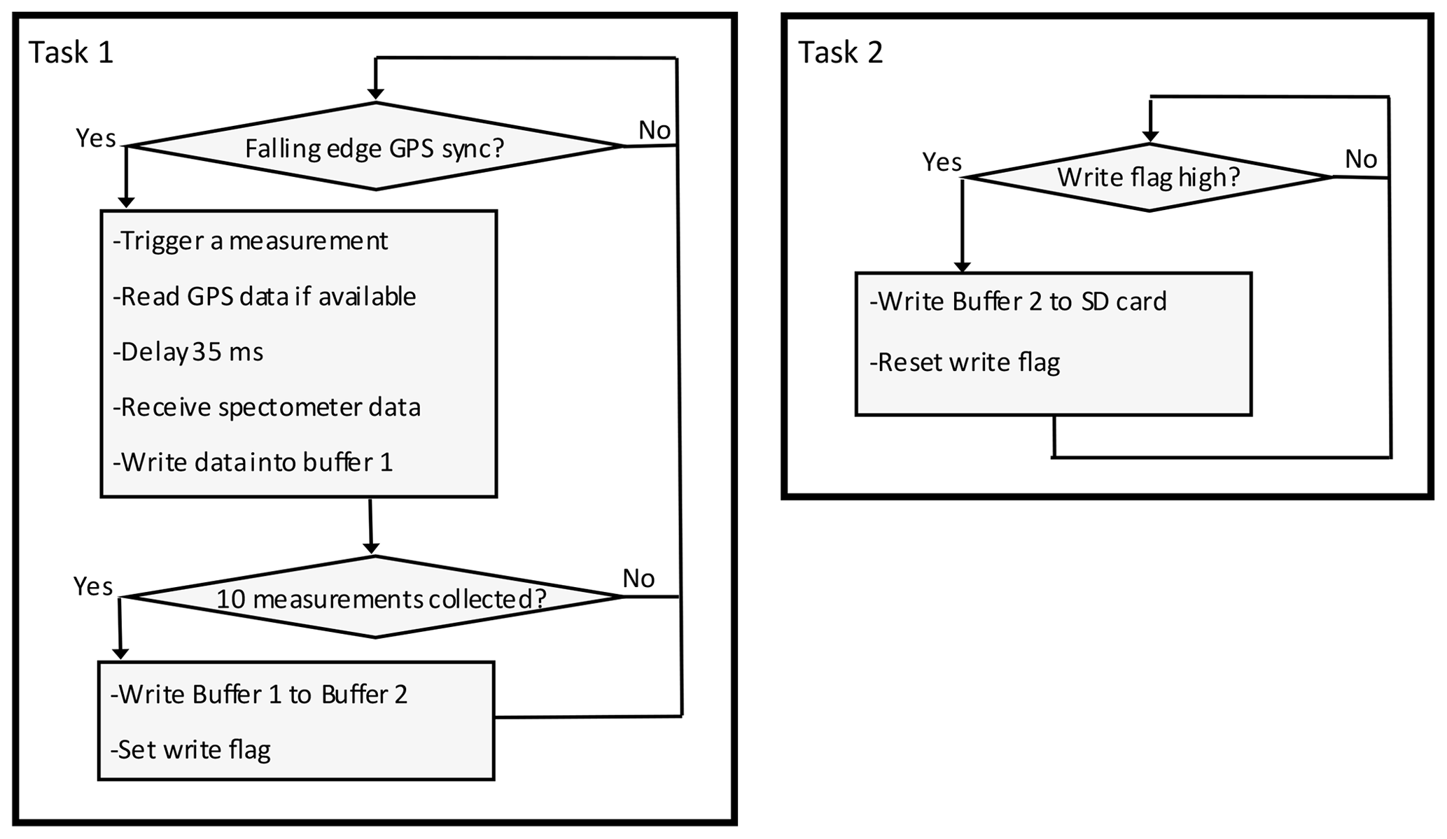
Figure 3 Multitasking software implementation for synchronized measurements and data storage. Each buffer can contain 10 rows of data. The program is available at Zenodo (https://doi.org/10.5281/zenodo.6945812, Heusinkveld, 2022).

For data logging, the MKR Zero of the Arduino family microprocessor platforms was chosen. It is a cost-effective and low-power data-logging solution using a 48 MHz SAM D21 Cortex 32 bit low-power ARM MCU and a built-in microSD card holder (max 32 GB). A consumer-grade 32 GB SD card was selected, data rates are low (< 5 kB s⁻¹), and the large size ensures that the card does not wear down fast (< 4 GB per month). The challenge with this data-logging solution is that the default operating system cannot handle sustained data writing to an SD card at 10 Hz using linear programming (despite a low data rate of < 5 kB s⁻¹). In fact, the SD card would regularly delay the measurements by an estimated 200 ms, resulting in a loss of data (tested with a new, fast SD card with 85 MB s⁻¹ max write speed). Thus a microcontroller multitasking real-time operating system is needed, and FreeRTOS (http://freertos.org, last access: 27 July 2023, FreeRTOS_SAM21 by BriscoeTech, version 2.3.0) was chosen to overcome this challenge. Two tasks that run semi-parallel on the single-core CPU were defined. The first task with the highest priority will initiate a measurement cycle at the falling edge of the hardware timing signal of the GNSS. Task 2 will be triggered each second and writes the 10 Hz buffered data to the SD card (Fig. 3).

2.6 Field experiments

The field experiments were conducted at various locations. At the Veenkampen weather station, Wageningen, the Netherlands (lat 51.981^∘, long 5.620^∘), sensor performance was tested against GHI measurements and a spectrophotometer. Although GHI is directly measured with a pyranometer, it was decided to use the pyrheliometer and diffuse radiation sum to reduce cosine response errors. The instruments consist of a Kipp & Zonen pyrheliometer CHP1 with a calibration accuracy of ±0.5 % and a first-class pyranometer CM 21 for diffuse radiation measurements with a time constant of 5 s, directional error < ±10 W m², tilt error ±0.2 %, zero-offset due to T change < 2 W m² at 5 K h⁻¹, and cosine response error max ±2 % at 60^∘ and max ±6 % at 80^∘. Both instruments were mounted on a sun tracker (EKO Instruments, Japan, STR-21 with shading disk). On selected days the solar spectrum was measured with an ASD FieldSpec (USA) field spectroradiometer with a cosine collector and with a factory recalibration performed in 2021.

Additionally, a large set of sensors were deployed during the FESSTVaL campaign (https://fesstval.de/, last access: 27 July 2023) at the German Weather Service (DWD) in Falkenberg, Germany, to study the spatial variation in solar irradiance (June 2021). For that campaign, it was crucial to obtain fast and time-synchronized spatial solar irradiance measurements. Their Baseline Surface Radiation Network (BSRN) location at Lindenberg (Driemel et al., 2018) was used to test long-term stability from 22 June–31 August 2021.

FROST was also deployed in a field experiment in La Cendrosa, Spain (lat 41.692537^∘, long 0.931540^∘) from 14–29 July 2021. It was used, among other things, to study crop growth.

3 Performance and applications

The performance of the sensor, the temperature dependency and cosine response of the diffuser, and the time synchronization are presented below. The infrared crosstalk is analyzed by measuring signal response with all light below 1000 nm blocked using a low-pass infrared filter. Subsequently a correction method using heat-absorbing infrared filters (referred to as “correction filters”) is introduced and tested. This results in three versions of FROST: one with a 10.6 mm diffuser, one with a 2 mm diffuser including a correction filter on the blue sensor, and one with a 2 mm diffuser with two correction filters (on the blue and red sensor).

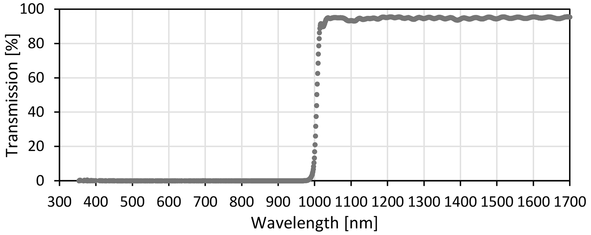
Figure 4 Transmission of the optical LP filter measured with a Cary 5000 UV–Vis–NIR spectrophotometer equipped with a universal measurement accessory at the DWD, Lindenberg, Germany.

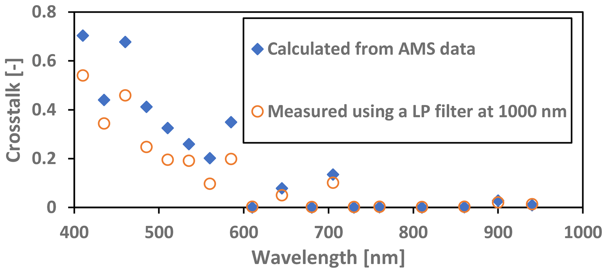
Figure 5 Measured spectroscopy sensor infrared crosstalk from wavelengths > 1000 nm, tested with a xenon lamp and an optical long-pass filter (LP at 1000 nm) and calculated from spectral-response data as supplied by the manufacturer (AMS). Crosstalk is defined as the fraction of light wavelengths > 1000 nm that the sensor is responding to; for example at 410 nm, 55 % of the measured signal actually originates from wavelengths > 1000 nm.

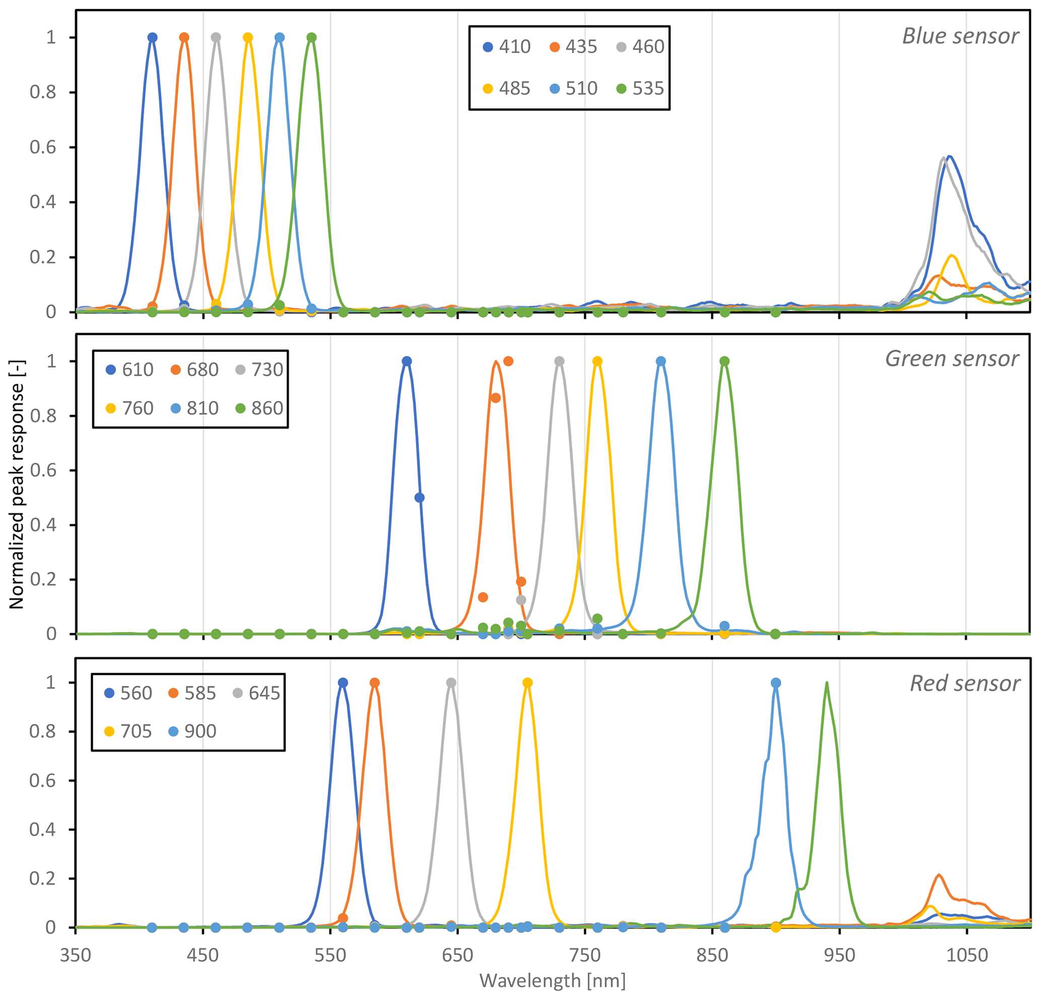
Figure 6 Normalized peak spectral response of the triple AMS sensor (denoted as blue, green, and red sensor); data provided by manufacturer after consultation (solid lines) and our measured response up to 900 nm (dots) as measured with a sensor placed inside a Cary 4000 UV–Vis spectrophotometer equipped with a universal measurement accessory.

3.1 Spectral response and calibration

According to the manufacturer specifications, the normalized (at peak wavelength) responsivity of their spectroradiometer has a good narrow-band response (20 nm FWHM) and limited overlap for the 18 channels. Wavelength accuracy is within ±10 nm, and this was confirmed by testing the sensor inside a Cary 4000 UV–Vis spectrophotometer equipped with a universal attachment accessory. Unfortunately, the Cary spectrophotometer had a limited spectral range; thus, we were unable to test the crosstalk in the near infrared or test the 940 nm band (Fig. 6).

Linearity was tested by comparing the spectroradiometer against a reference thermopile pyranometer CM 21 (Kipp & Zonen, the Netherlands) and a stabilized halogen light source in a darkroom. The intensity was adjusted by changing the lamp distance. The FROST non-linearity was at least as good as the CM 21, which has a non-linearity of < ±0.2 %. The factory-calibrated accuracy is ±12 % according to the manufacturer specifications (35 counts µW⁻¹ cm²). After initial testing using solar radiation as a light source for reflectance measurements of lawn grass, we were confronted with unusual data. The PAR region clearly showed very high reflection values, more than 5 times what is typical of such a surface.

After consultation with the manufacturer (AMS), they clarified that the AS72653 sensor has a strong crosstalk in the near infrared. The sensor was meant to be used with LED light for spectral reflectance measurement applications, which would not produce light > 1000 nm. They recommend a specific LED for each sensor, and therefore each reflectance measurement would consist of three separate measurements with each using one sensor and with one specific LED at a time.

We tested the sensor at the DWD radiation calibration facility in Lindenberg using a calibrated light source. The crosstalk caused by light wavelengths beyond 1000 nm was measured by using an optical long-pass (LP) interference filter that blocks all light below 1000 nm. Thus, the remaining signal on all 18 channels can be attributed to crosstalk from wavelengths > 1000 nm. The blocking filter characteristics were tested in a Cary 5000 UV–Vis–NIR spectrophotometer equipped with a universal attachment accessory (Fig. 4).

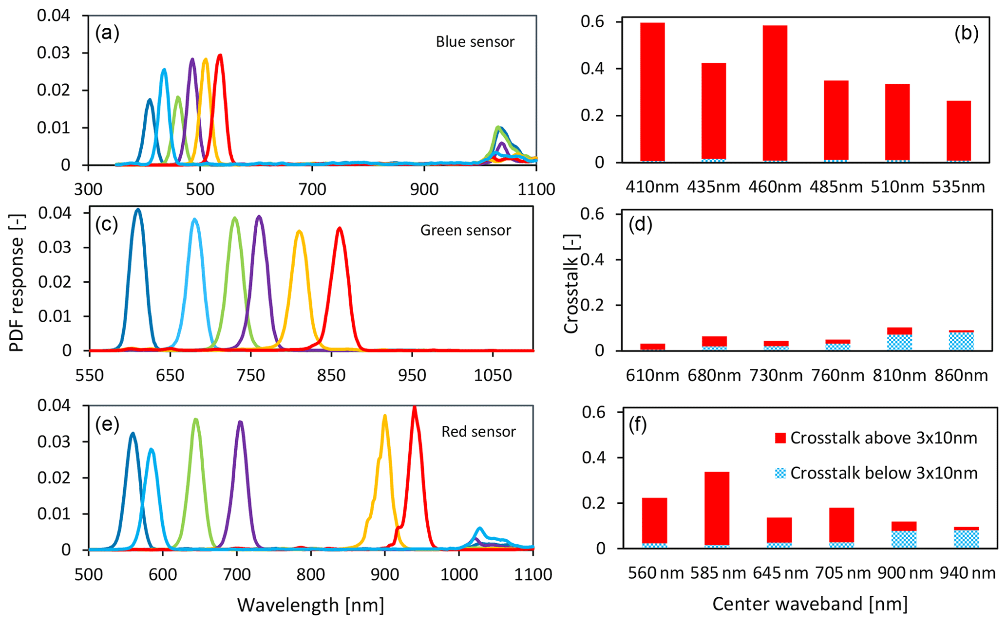
Figure 7 (a, c, e) Spectral response of the triple AMS sensor (denoted as blue, green, and red sensor), Probability density functions (PDFs) calculated from data provided by the manufacturer AMS (Kumud Dey, personal communication, 2020). (b, d, f) The crosstalk for each channel is presented as two values: signal originating from > (center wavelength + 30 nm) divided by total signal of a channel (red) and signal < (center wavelength − 30 nm) divided by total signal of a channel (blue) (sensor only, without diffuser).

Figure 5 shows the fraction of infrared light (> 1000 nm) within the sensor output for each of the 18 channels. The sensor output was corrected for the LP filter transmission loss (about 5 %; see Fig. 4). Note that the crosstalk is larger than during solar radiation measurements because a xenon light source contains a higher amount of infrared radiation. Cloudy conditions would further reduce crosstalk. For clear-sky conditions, the crosstalk would be about half of the xenon light. The blue diamonds in Fig. 5 show the calculated crosstalk using the AMS sensor spectral filter response data obtained through personal communication (Kumud Dey, personal communication, 2020) with the manufacturer (Fig. 6). The measured crosstalk on the blue sensor appears to be slightly better. The crosstalk is very large in the visible light range and confirms the provided filter transmission curves from AMS (Kumud Dey, personal communication, 2020​​​​​​​). Note that those transmission curves (Fig. 6) are not available on the publicly available datasheet. Figure 5 shows that only half of the channels provide the correct spectral information (if calibrated correctly using the data from Fig. 6). However, there are enough channels to measure the so-called red edge around 700 nm in vegetation light transmission and reflection. This opens up applications for vegetation growth measurements without further modifications.

All channels in the blue sensor and some of the channels (650 and 685 nm) in the red sensor have very high crosstalk from the 1000-to-1100 nm range, but the crosstalk makes the sensor cover a larger range of the solar spectrum. It is therefore still usable if this can be quantified.

In Fig. 7, the right panels show that the crosstalk for a flat spectrum, defined as the signal above or below 3×0.5 FWHM from the center wavelength, is large (up to 60 %) in the PAR range for the blue sensor and mainly from the infrared beyond 1000 nm. The green sensor performs much better and exhibits minimal infrared crosstalk (< 5 %). The red sensor has an issue mainly with the first two channels.

To remove infrared crosstalk, an optical short-pass filter is required. However, a filter with a sharp cutoff at 1000 nm is, to our knowledge, not available or probably very expensive and sensitive to the angle of incidence. Cost-effective short-pass filters are made from heat-absorbing glass and have a dye added to the glass that absorbs infrared radiation (Fig. 8). However, these heat-absorbing filters do not have a steep filter response and therefore are ineffective at correcting the red sensor without attenuating the 900 and 940 nm channels too much. The Schott heat-absorbing filters KG3 and KG1 appear to offer a good solution for the blue sensor (Fig. 9, second-row panels). The remaining crosstalk is mainly related to the slightly broader filter response. The first four channels of the red sensor (Fig. 7, lower panels) can also be improved. However, such a correction filter for the red sensor would increase crosstalk from shorter wavelengths for the 900 and 940 nm wavebands (see lower-right panel in Fig. 9) and greatly reduce signal strength. For accurate PAR measurements and when the 900 and 940 nm channels are not needed, using the weaker KG1 filter for the red sensor is recommended.

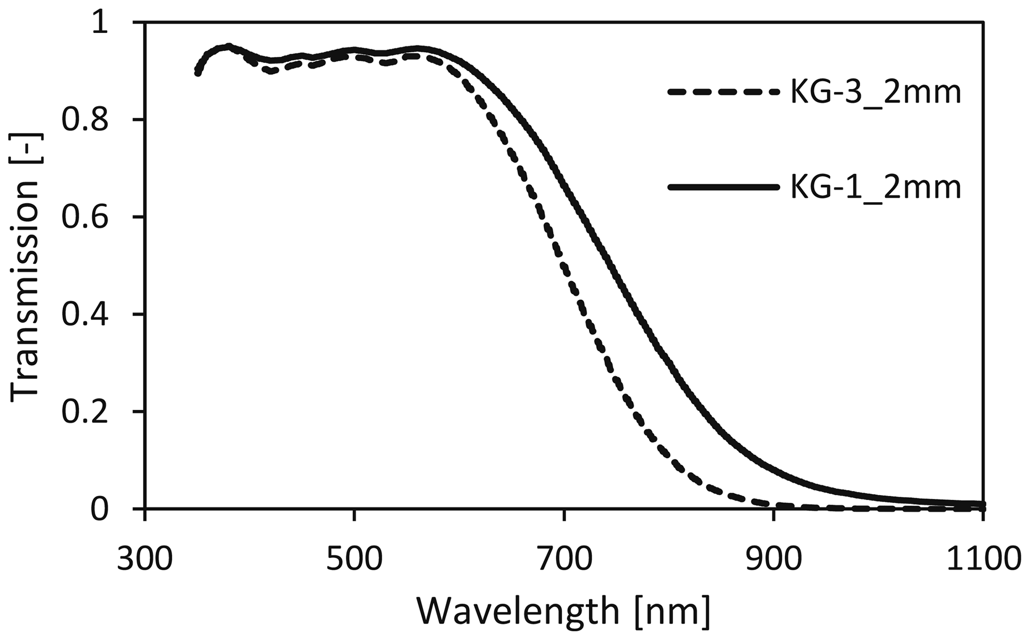
Figure 8 Correction filters for the infrared crosstalk: Schott heat-absorbing filters (adapted from Schott AG manufacturer data).

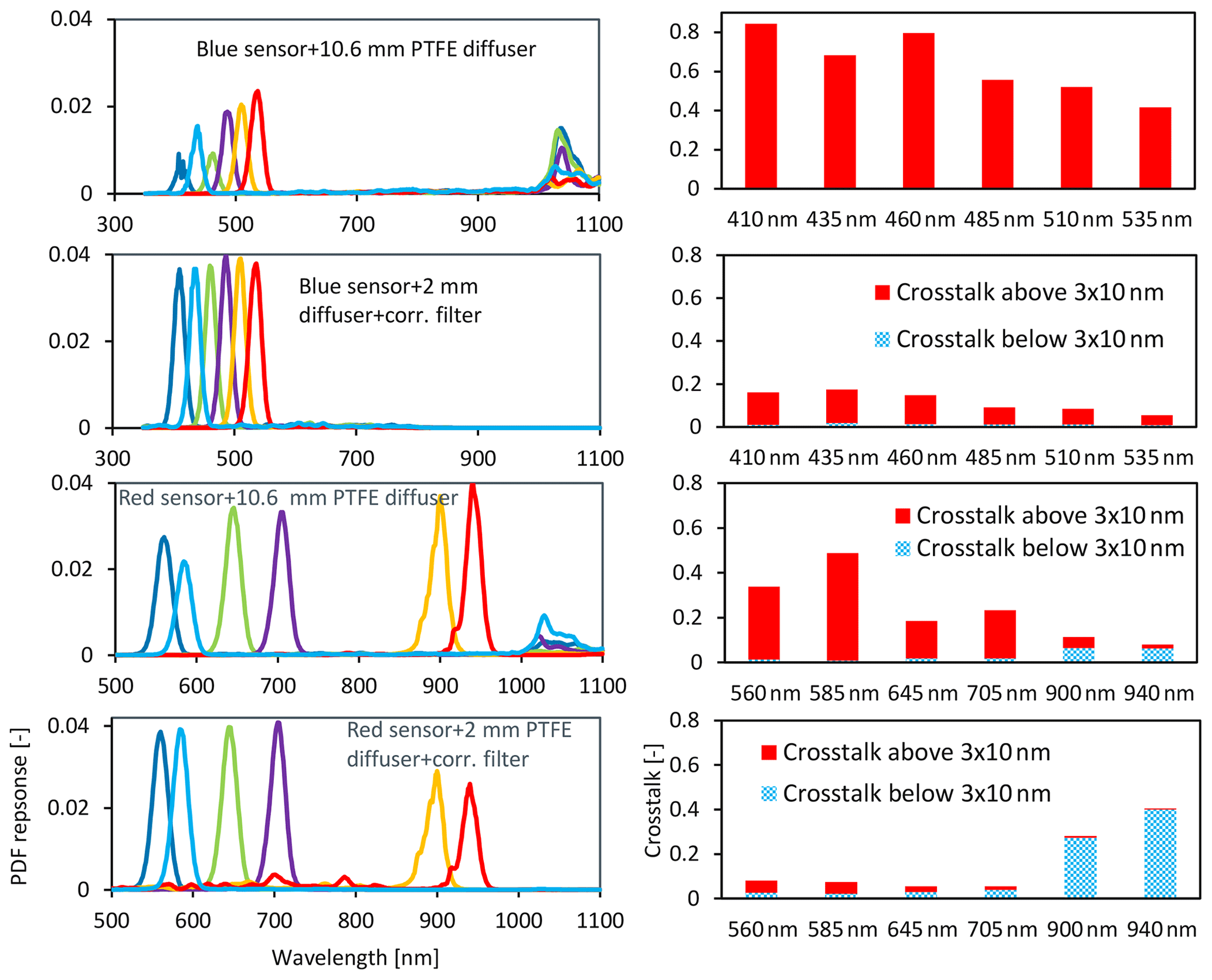
Figure 9 Spectral response and crosstalk (for a flat spectrum) of the blue and red sensor, without or with correction filter. First row: blue sensor with 10.6 mm PTFE diffuser. Second row: blue sensor with 2 mm PTFE diffuser including a heat-absorbing filter (Schott KG3). Third row: red sensor with 10.6 mm PTFE diffuser. Fourth row: red sensor with 2 mm PTFE diffuser and heat-absorbing filter (Schott KG1), calculated from manufacturer data of sensor spectral response, transmission data of the Schott optical correction filter, and measured transmission of PTFE diffusers.

Because of the limited view angle of the spectroscopy sensors (40^∘), it is crucial to add a light diffuser. Two light-diffusing materials were tested, PTFE and opal cast acrylic sheet glass, and the transmission measurements are shown in Fig. 10 (measured with the ASD FieldSpec).

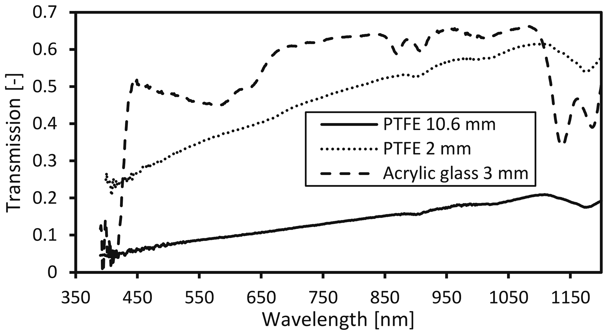
Figure 10 Transmission of PTFE diffusers and an opal cast acrylic sheet glass diffuser measured with an ASD FieldSpec spectroradiometer.

The reduced transmittance of the PTFE diffusers in the shorter wavelengths (Fig. 10) enhances the near-infrared crosstalk (compare Fig. 9 top-right panel with Fig. 7 top-right panel). The combined effect of sensor and PTFE spectral response with or without correction filters is shown in Fig. 11. Three versions of the spectrophotometer were developed: one with a 10.6 mm PTFE diffuser to improve cosine response (FROST1), a second version with a 2 mm PTFE diffuser and a correction filter on the blue sensor (FROST2), and a third version with a 2 mm PTFE diffuser and correction filters on the blue and red sensor (FROST3). The spectral selective quality on real-world measurements (Fig. 11) was calculated from the combined effect of the spectrophotometer filter characteristics (Figs. 7 and 8), diffuser (Fig. 10), and Schott correction filters (Fig. 8).

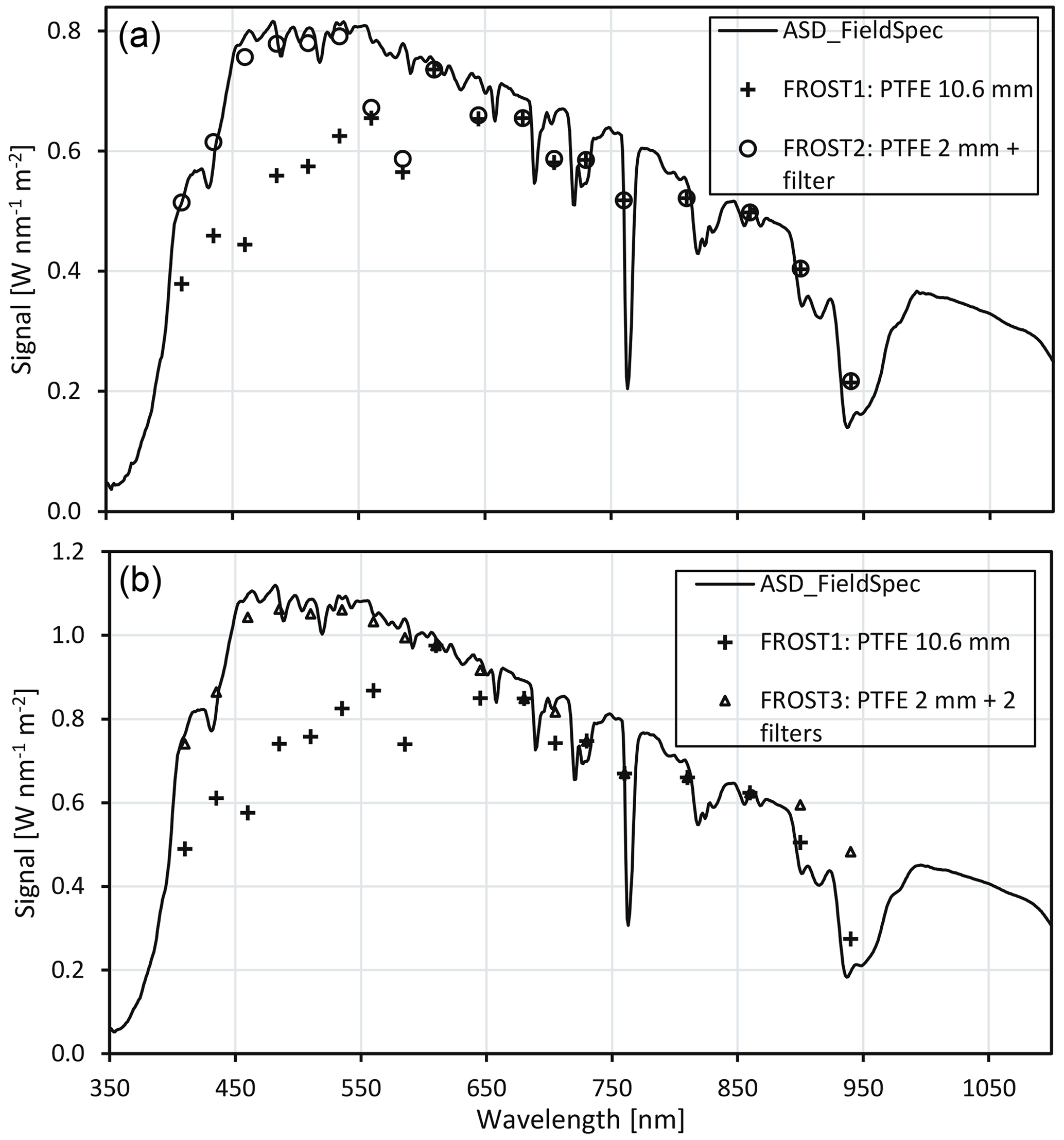
Figure 11 Outdoor measurements (ASD FieldSpec) with calculated response of three FROST versions: FROST1 with a 10.6 mm diffuser, FROST2 with a 2 mm PTFE diffuser and a correction filter on the blue sensor, and FROST3 with a 2 mm PTFE diffuser and a correction filter on the blue and red sensor, considering sensor spectral response and transmission of diffuser and correction filter, during clear-sky conditions, Wageningen: (b) 15 May 2022, 14:24 UTC; (a) 11 March 2022, 13:35 UTC.

Figure 11 shows that the first 8 channels, if uncorrected with a heat-absorbing filter, underestimate the irradiance levels at the expected wavebands because these bands are very sensitive to the infrared region between 1000 and 1100 nm. At this infrared region, the solar radiation intensity is lower than what the blue sensor is supposed to see and thus leads to an underestimation of the blue sensor for the visible channels. The heat-absorbing filters effectively remove this crosstalk. It also shows that the red sensor benefits from a heat-absorbing filter for the wavebands 560 and 585 nm, but it greatly reduces the sensitivity of the 900 and 940 nm wavebands, which makes the contribution of crosstalk from short wavebands too high (large positive deviation). Therefore the red sensor should not be equipped with such a filter if the 900 and 940 nm wavebands are important, for example to estimate column atmospheric moisture (see Fig. 17).

The procedure to calibrate each waveband of FROST would require an accurate spectrophotometer and a clear day. First, each of the 18 PDF band responses of the sensor (with or without a correction filter!) and diffuser combinations is multiplied with the known solar spectrum for a very clear day or measured with a calibrated spectrophotometer. This gives the nW m⁻² reference value that the FROST sensor should produce for each waveband. Subsequently the 18 raw FROST wavebands' outputs are multiplied by the AMS calibration factors (since we use the uncalibrated output for fast measurement) and divided by the reference values. The AMS spectroscopy sensor factory calibration values are written to the SD card at the very start of the measurements. The derivation of the calibration values for each FROST channel i in counts W⁻¹ m² can be written as

$$\begin{array}{}\text{(1)}& {\mathrm{Cal}}_{\mathrm{FROST},i}={\displaystyle \frac{{\mathrm{Counts}}_i\cdot {\mathrm{Cal}}_{\mathrm{manufacturer},i}}{{\sum }_{{\mathit{\lambda }}_{\mathrm{1}}}^{{\mathit{\lambda }}_{\mathrm{2}}}\left[\frac{R_{{\mathrm{sensor}}_{i,\mathit{\lambda }}}\cdot T_{{\mathrm{diffuser}}_{\mathit{\lambda }}}\cdot T_{{\mathrm{filter}}_{\mathit{\lambda }}}}{{\sum }_{{\mathit{\lambda }}_{\mathrm{1}}}^{{\mathit{\lambda }}_{\mathrm{2}}}{R}_{{\mathrm{sensor}}_{i,\mathit{\lambda }}}\cdot T_{{\mathrm{diffuser}}_{\mathit{\lambda }}}\cdot T_{{\mathrm{filter}}_{\mathit{\lambda }}}}\cdot {\mathrm{Source}}_{\mathit{\lambda }}\right]}},\end{array}$$

where Counts_i is the signal output of a FROST channel i, from 1 to 18 (–); Cal_{manufacturer,i} is the manufacturer calibration factor (–) for channel i; $R_{{\mathrm{sensor}}_{i,\mathit{\lambda }}}$ is the normalized peak spectral response of channel i (–) at wavelength λ (nm); $T_{{\mathrm{diffuser}}_{\mathit{\lambda }}}$ is the spectral transmission of the diffuser (–) at wavelength λ (nm); $T_{{\mathrm{filter}}_{\mathit{\lambda }}}$ is the transmission of the (optional) crosstalk correction filter (–) at wavelength λ (nm); Source_λ (W m⁻²) is the output of the reference light source at wavelength λ (nm) (preferably the sun); and λ₁ and λ₂​​​​​​​ are the lower and upper boundaries of the spectral sensitivity range (including crosstalk) of FROST. Note that the denominator is the spectrally weighted source signal strength.

Table 2 Sensitivity, or counts (C) W⁻¹ m² of FROST1, FROST2, and FROST3 with different configurations; offsets are always zero. Every sensor uses a gain of 16 and an integration time of 13.9 ms. The flags denote quality of measurement (waveband accuracy). Flag 0: low crosstalk; Flag 1: crosstalk < 20 %; Flag 2: 20 % < crosstalk < 35 %; Flag 3: crosstalk > 35 %. The colors in the first column indicate each of the three sensors in FROST. The final column shows the improvement factor for sensitivity when using a 3 mm white acrylic glass diffuser instead of a 2 mm PTFE diffuser.

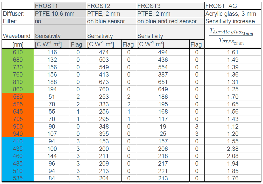
The sensor output sensitivity is then expressed as counts W⁻¹ m². The normalized sensor response is provided in Figs. 7 and 9 and in Table S1 in the Supplement. An example of sensitivity values is presented in Table 2. These values were derived on 11 March 2022 at 13:35 UTC for the 10.6 mm diffuser version and the 2 mm diffuser + one filter version. The 2 mm diffuser with two correction filters was measured on 15 May 2022 (Fig. 11). Note that these values are only valid for an integration value of 13.9 ms and a gain of 16. We do not recommend using channels with Flag 2 or 3 if spectral accuracy is required.

3.2 Temperature sensitivity and drift

The diffuser and sensor were both tested for temperature effects. The measurements were corrected for sensor temperature drift or drift in lamp output by measuring the lamp output with an extra sensor outside the oven. The oven has an internal fan to assure a homogeneous temperature within the oven chamber. The PTFE filter shows a significant jump in transmission around 21 ^∘C; then it reaches a plateau and slowly declines past 35 ^∘C (Fig. 12, upper panel). The temperature was slowly increased and stabilized for 30 min at each measurement point to minimize thermal delays in the PTFE material.

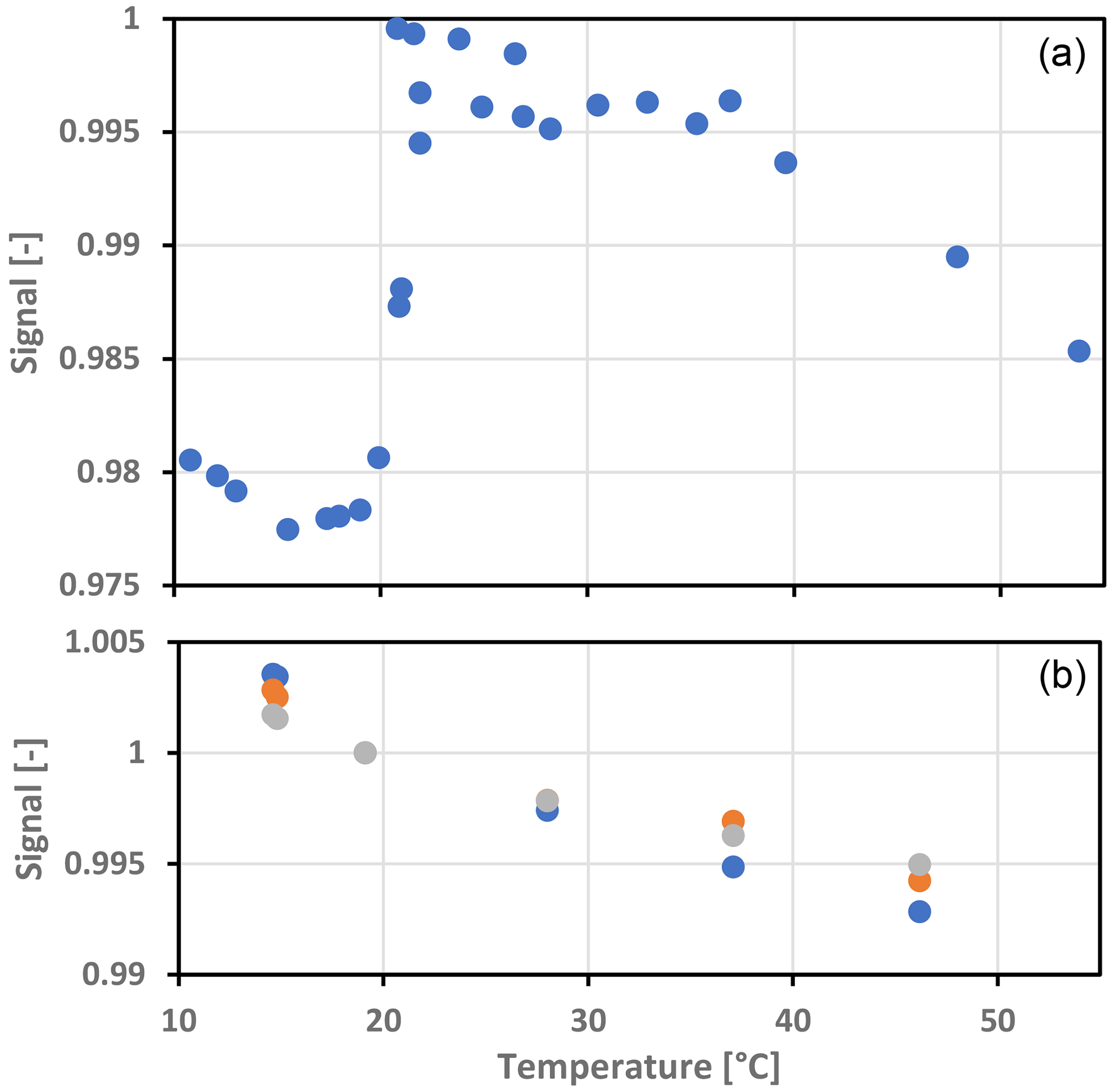
Figure 12 Temperature response: (a) PTFE diffuser and (b) three random light sensors (−250 ppm).

Three spectroscopy sensor chipsets (3 × 18 wavebands) were oven-tested for temperature sensitivity between 16 and 46 ^∘C. Overall temperature sensitivity is −250 ppm K⁻¹ with a small variation among the three sensors. Lower temperatures were not possible due to condensation issues when reaching the dew point temperature of the laboratory (Fig. 12).

3.3 Cosine response and GHI

The cosine response measurements (outside, LED lamp) had a better performance for the 10 mm diffuser but nevertheless had some inconsistencies among the three sensors. We tried to improve the cosine response by leaving part of the sides uncovered, but this caused a very high asymmetry among the three sensors. The explanation is that the three sensors do not have the same viewing angle location under the diffuser; thus some will see more from the side than the other sensors. The side sensitivity is greatly reduced with a thinner filter but at the expense of a reduced cosine response (Fig. 13).

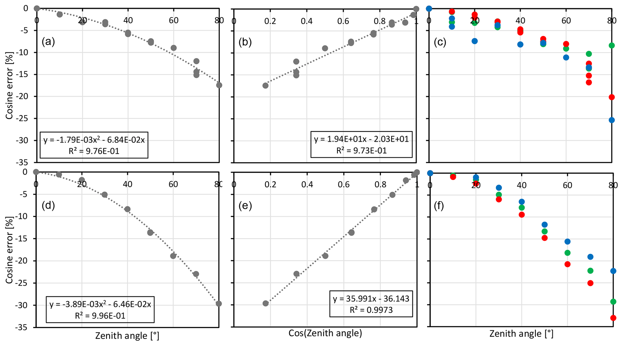
Figure 13 (a–c) The 10.6 mm diffuser (black sides). (d–f) The 2 mm diffuser (sides painted black). Panels (c) and (f) are color-coded for each sensor integrated circuit.

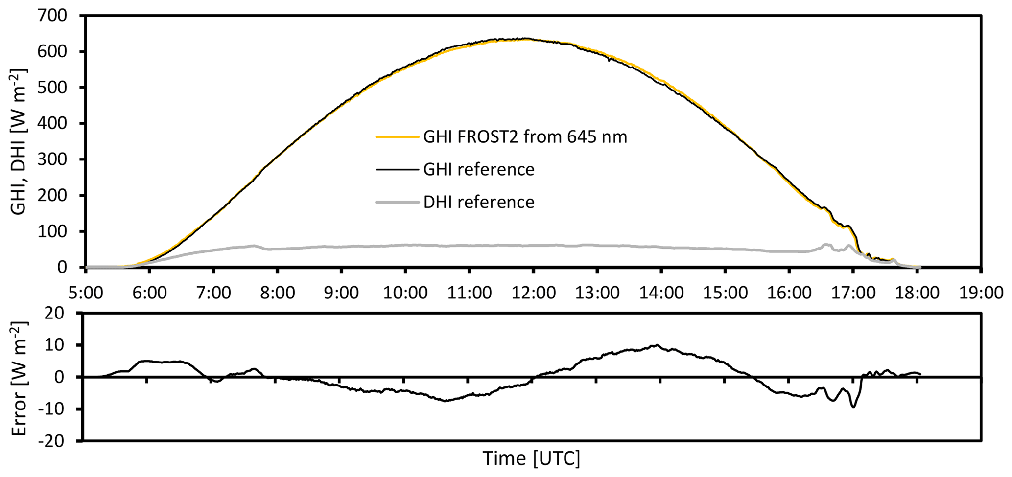
Figure 14 Comparison between GHI measured using a pyrheliometer and diffuse radiation sum (on a sun tracker and correcting for zenith angle) and a calibrated FROST2 with a 2 mm PTFE diffuser and one correction filter; diffuse horizontal irradiance (DHI) measured with a pyranometer mounted on a sun tracker with a shading ball, Veenkampen weather station, 19 March 2022. Relative errors at GHI > 200 W m⁻² are < 2 % and mainly related to horizontal misalignment causing an asymmetric error before/after noon UTC.

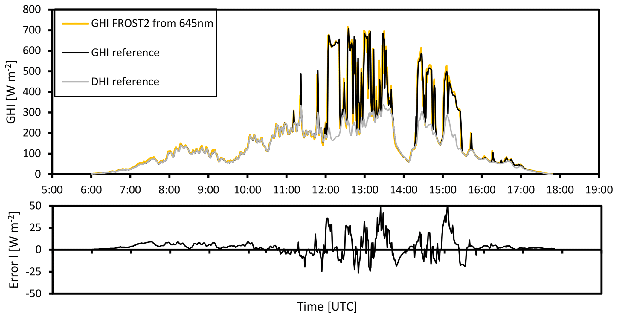
Figure 15 Calibrated FROST2 GHI from 645 nm (calibrated on a clear day, 19 March; see Fig. 14); calibration tested with cloudy weather conditions – cloudy weather conditions in the morning, some clearing in the afternoon, 1 min averaged data, error plot 10 min running mean to suppress differences due to spatial separation of FROST and reference (145 m apart), Veenkampen weather station, 14 March 2022. Relative errors at GHI > 100 W m⁻² are < 7 % and mainly related to spatial separation between FROST and reference.

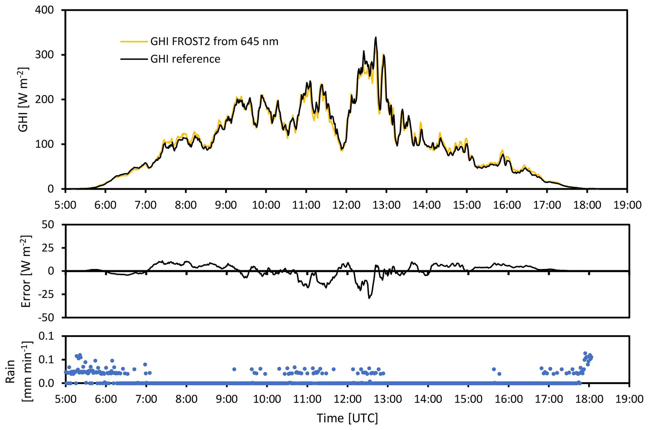
Figure 16 Calibrated FROST2 GHI from 645 nm (calibrated on a clear day, 19 March; see Fig. 14); calibration tested under rainy weather conditions, 1 min averaged data, error plot 10 min running mean to suppress differences due to spatial separation of FROST and reference (145 m apart), Veenkampen weather station, 31 March 2022. Relative errors at GHI > 100 W m⁻² are < 7 % and mainly related to spatial separation between FROST and reference.

We found that most of the cosine response errors can be corrected afterwards and is demonstrated for the 2 mm filter, which had the largest cosine response error but less transmission loss. The accurate measurement of GHI can be achieved by first correcting for the zenith angle response (see Fig. 13, lower-middle panel) and subsequently applying a second-order linear regression against a reference pyranometer on 1 clear day (19 March 2021). Additionally, a correction for the limited spectral response is needed. We tested this calibration method for the average signal of all 18 wavebands and on single wavebands. The dataset contains clear-sky days (Fig. 14), overcast days (Fig. 15), and rainy weather (Fig. 16). The best overall results were achieved with either channel 645 or channel 705 nm, with residual errors mainly below 10 W m⁻² during contrasting weather conditions. Due to the spatial separation of 156 m between our sensors and the reference solar radiation measurements and the differences in response speed, we rejected the cloud passage time intervals. The 645 and 705 nm wavebands seem to correct cloud effects on the GHI where irradiance is enhanced below 500 nm and reduced due to water absorption bands at wavebands > 1 µm.

The remaining uncertainty in the clear-day calibration (up to 10 W m⁻² or 5 %) is mainly related to small leveling uncertainties or tolerances in input optics of both the reference and our sensors. This is visible as a shift from a negative to a positive bias around 12:00 UTC (Fig. 14).

The instruments were not dried during the precipitation event (Figs. 16 and 17). Water droplets on the diffuser may affect light transmission and diffuser optical properties. Note that in Figs. 14–16, the nocturnal offsets are zero.

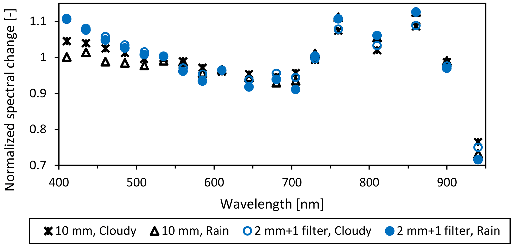
Figure 17 Two FROST instruments, one with a 10 mm diffuser (FROST1) and one with a 2 mm diffuser and correction filter (FROST2). The normalized spectral cloud modification factor is the spectral change in cloudy (14 March 2022) and rainy weather (31 March 2022) compared to a cloud-free day (19 March 2022), Veenkampen weather station, data averaged between 11:00 and 12:00 UTC for each day.

Next, we investigated how the light spectra are modified by clouds or rain. The two instruments, one with a 10 mm diffuser (FROST1) and the second version with a 2 mm diffuser and crosstalk correction filter on the blue sensor (FROST2), were used to calculate the spectral change due to cloudy or rainy weather conditions (Eq. 2).

$$\begin{array}{}\text{(2)}& \mathrm{Spectral}\mathrm{\_}{\mathrm{change}}_i={\displaystyle \frac{\frac{{\mathrm{Counts}}_{i,\mathrm{clouds}\mathrm{\_}\mathrm{rain}}}{\frac{\mathrm{1}}{\mathrm{18}}\sum _{i=\mathrm{1}}^{\mathrm{18}}{\mathrm{Counts}}_{i,\mathrm{clouds}\mathrm{\_}\mathrm{rain}}}}{\frac{{\mathrm{Counts}}_{i,\mathrm{clear}}}{\frac{\mathrm{1}}{\mathrm{18}}\sum _{i=\mathrm{1}}^{\mathrm{18}}{\mathrm{Counts}}_{i,\mathrm{clear}}}}}\end{array}$$

Data from the experiments shown in Figs. 14–16 were used, and, of the 3 contrasting days, the 11:00–12:00 UTC intervals were averaged and normalized for the average spectral signal of the 18 wavebands. Figure 16 shows that the 940 nm waveband is very sensitive to moisture, with a reduction of more than 20 % as compared to its nearest waveband. Accordingly, it can be used to derive information about atmospheric moisture such as column water vapor. Both cloudy and rainy conditions appear to modify the spectra in a similar way (Fig. 17). The low enhancement in the first four wavebands of the instrument with the 10 mm diffuser version (FROST1) is related to the strong crosstalk in the near infrared. The corrected version with the 2 mm diffuser (FROST2), which contains the crosstalk correction filter, shows an enhancement due to clouds and is in line with the findings by Durand et al. (2012), who had an enhancement below 465 nm. The 645 or 705 nm waveband as shown in Figs. 14–16 appears to have the right amount of sensitivity reduction due to clouds and rain (slightly stronger) to be used for GHI measurements. It is, however, recommended to use all 18 bands and use a proper weighting function that reduces sensitivity in the visible region. We currently have no explanation for the enhancements between 750 and 860 nm.

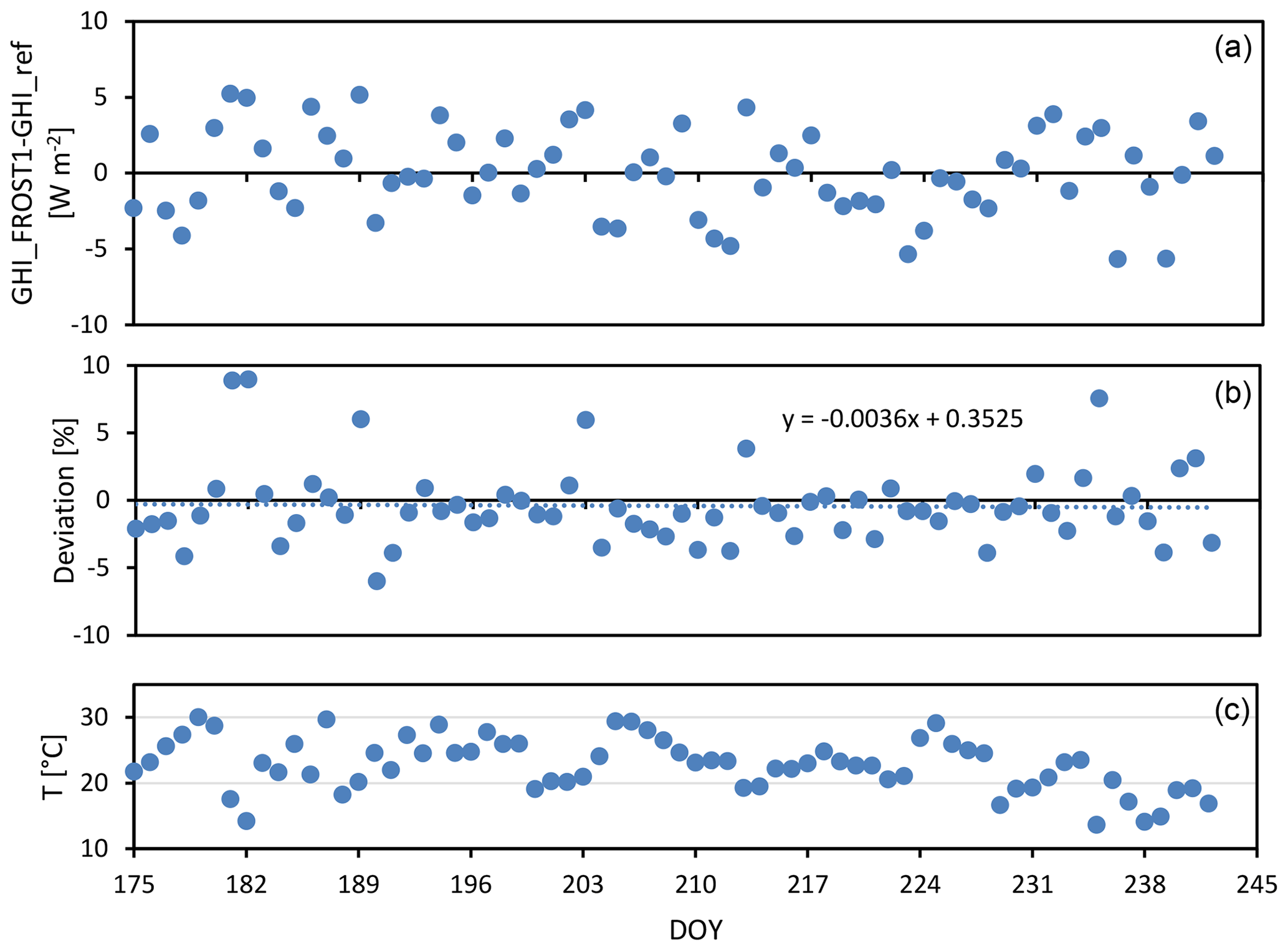
Figure 18 Long-term stability of FROST1 GHI measurements (using the 645 nm channel and calibrated with day of year (DOY) 226, 14 August 2021 data). (a) Daily average FROST GHI deviation from reference GHI. (b) FROST1 GHI deviation from averaged data between 12:00 and 13:00 UTC. (c) Average air temperature between 12:00 and 13:00 UTC, during a 2.5-month comparison experiment at Lindenberg. Measurements corrected for PTFE diffuser transmission change at 21 ^∘C.

The long-term drift was tested at the Lindenberg rooftop observatory. One instrument was measuring from 22 June to 31 August 2021 (without any missing 0.1 s measurements). These data from 2.5 months were converted to GHI values by using only 1 relatively clear day (13 August) and compared with their reference pyranometer. The GHI standard error was 2.5 W m⁻² for daily averages with a diffuser temperature correction obtained by increasing sensor values by 2 % at temperatures below 21 ^∘C according to Fig. 12 and cosine response correction according to Fig. 13b (for daily errors see Fig. 18, upper panel). Additionally, the GHI deviations in percentage between 12:00 and 13:00 UTC were averaged to reveal possible sensor drift in time. The diffuser temperature correction practically removed all long-term drift (Fig. 18, middle panel).

3.4 Spatial measurements and synchronization

For spatial measurements, exact synchronization is essential. Our GNSS solution uses the hardware timing pulse of the GNSS to trigger a measurement. To illustrate the synchronization performance, we set up three standalone FROST sensors and let them run for 1 h outdoors. We then placed them in a darkroom, and at 12:00:45.6 UTC an LED light source was switched on for 0.3 s. Figure 19 shows 1.1 s of collected 10 Hz data of the 610 nm waveband. The response appears instantaneous and perfectly synchronized. There is still an integration time for each measurement, and this was set at 13.9 ms for FROST s16 and s20 and, for testing purposes, twice as long for the experimental version with a less transparent diffuser to get more signal. This instrument is denoted with “Exp” in Fig. 19. Therefore, the “Exp” FROST occasionally showed a small delay and illustrates the importance of configuring all sensors with the same integration time. Figure 19 also shows that the instruments have no zero-offset (no dark current) errors.

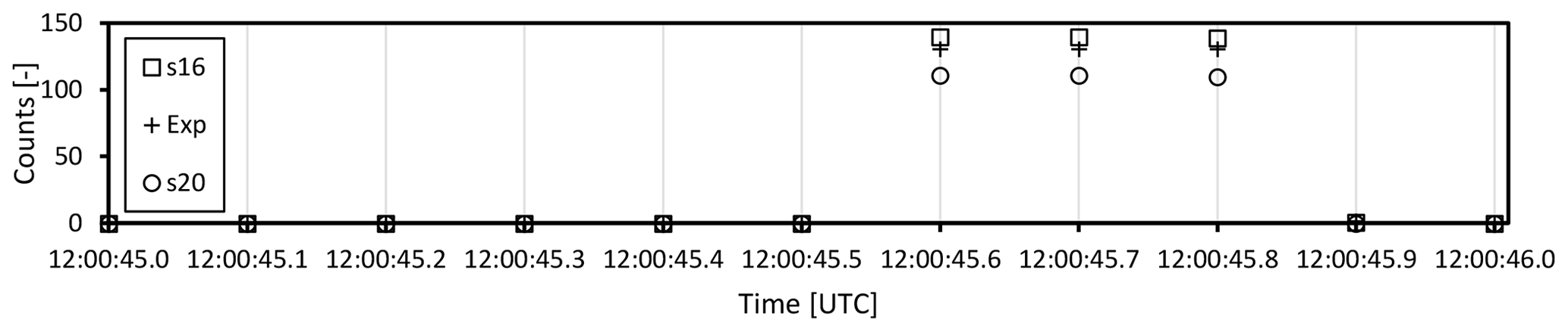
Figure 19 Example of synchronization, response speed, and zero offsets of three standalone instruments (uncalibrated). All three use their own GNSS for synchronization. Light pulse of 0.3 s generated by an LED lamp.

Table 3 Readout order during one full measurement cycle.

The full sensor readout requires two integration cycles with each cycle measuring 12 channels (see Table 3). As a result, there is a maximum of one integration cycle delay between certain channels (with our default settings: maximum 28 ms). Six channels are measured twice within one default measurement cycle (Table 3). For critical synchronization applications, it is possible to measure only 12 of the 18 channels during each measurement cycle.

The downside of a fast integration cycle is a smaller output signal. The 10.6 mm diffuser reduces the light onto the detector significantly, approximately 120 to 30 counts per channel at 650 W m⁻². The 2 mm diffuser increases the signal by a factor of 4. Longer integration times are considered but should be less than 50 ms to assure a sustained 10 Hz output (two integration cycles < 100 ms). Additional time is needed for data communication. The AMS spectroscopy sensor output is in ASCII format, and therefore more digits require more time to transmit.

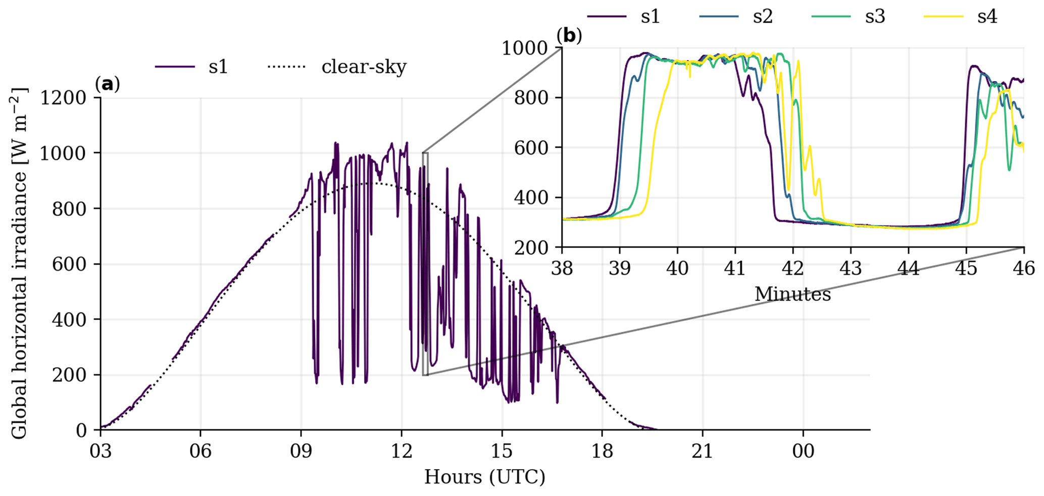
Figure 20 Measurements at 10 Hz of spatial variation in GHI at four locations along a 150 m west–east transect (b) compared to one location (a) at 1 min averages. The dashed line shows the CAMS McClear clear-sky product. Falkenberg, 27 June 2021.

For the measurement campaign in Falkenberg, a large 2-D sensor grid was deployed with 50 m grid spacing. It is a good illustration of the spatial dynamics of GHI during partly cloudy conditions. The 1 min averaged data at one point show the cloud enhancements, and the 10 Hz measurements show the high dynamics and spatial variation along a 150 m transect (Fig. 20).

3.5 Photosynthetic active radiation

Sensors for measuring photosynthetic active radiation (PAR) are usually constructed using a silicon photodiode and a light bandpass filter from 400 to 700 nm. Photosynthesis is a quantum process, and therefore measurements are usually expressed as a photosynthetic photon flux density (PPFD, µmol photons m⁻² s⁻¹). The sensor therefore must account for the larger number of photons at larger wavelengths. The wavelength sensitivity (in W m⁻² nm⁻¹) is such that the sensitivity at the 700 nm wavelength is 1.75 times larger than at 400 nm. In our case, we have 11 well-defined wavebands within the PAR region. Therefore, a digital filter can be used to calculate PPFD. Since the sensor outputs in W m⁻² nm⁻¹, it must be converted to PPFD by calculating the number of moles per joule per waveband.

The photon energy (E_n) at each waveband (n) is related to wavelength (λ) by the speed of light (c) and the Planck constant (h): $E_n=\frac{hc}{{\mathit{\lambda }}_n}$. The photons (P) per square meter are $P_n=\frac{R_n}{E_n}$, where R_n is the irradiance measured at each waveband. The number of moles is linked to the number of photons through Avogadro's number (A), and integration over all 11 FROST3 wavebands yields the total PPFD:

$$\begin{array}{}\text{(3)}& \mathrm{PPFD}=(\mathrm{700}-\mathrm{400})\underset{n=\mathrm{1}}{\overset{\mathrm{11}}{\int }}{P}_n/A{n}_{max}.\end{array}$$

The translation factor from W m⁻² nm⁻¹ to µmol m⁻² s⁻¹ nm⁻¹ for the 11 wavebands is depicted in Fig. 21. The PPFD in Fig. 11, lower panel, according to Eq. (3)​​​​​​​ is for example 1293 µmol m⁻² s⁻¹.

Figure 21 Conversion factor for each FROST3 waveband to calculate PPFD (µmol m⁻² s⁻¹).

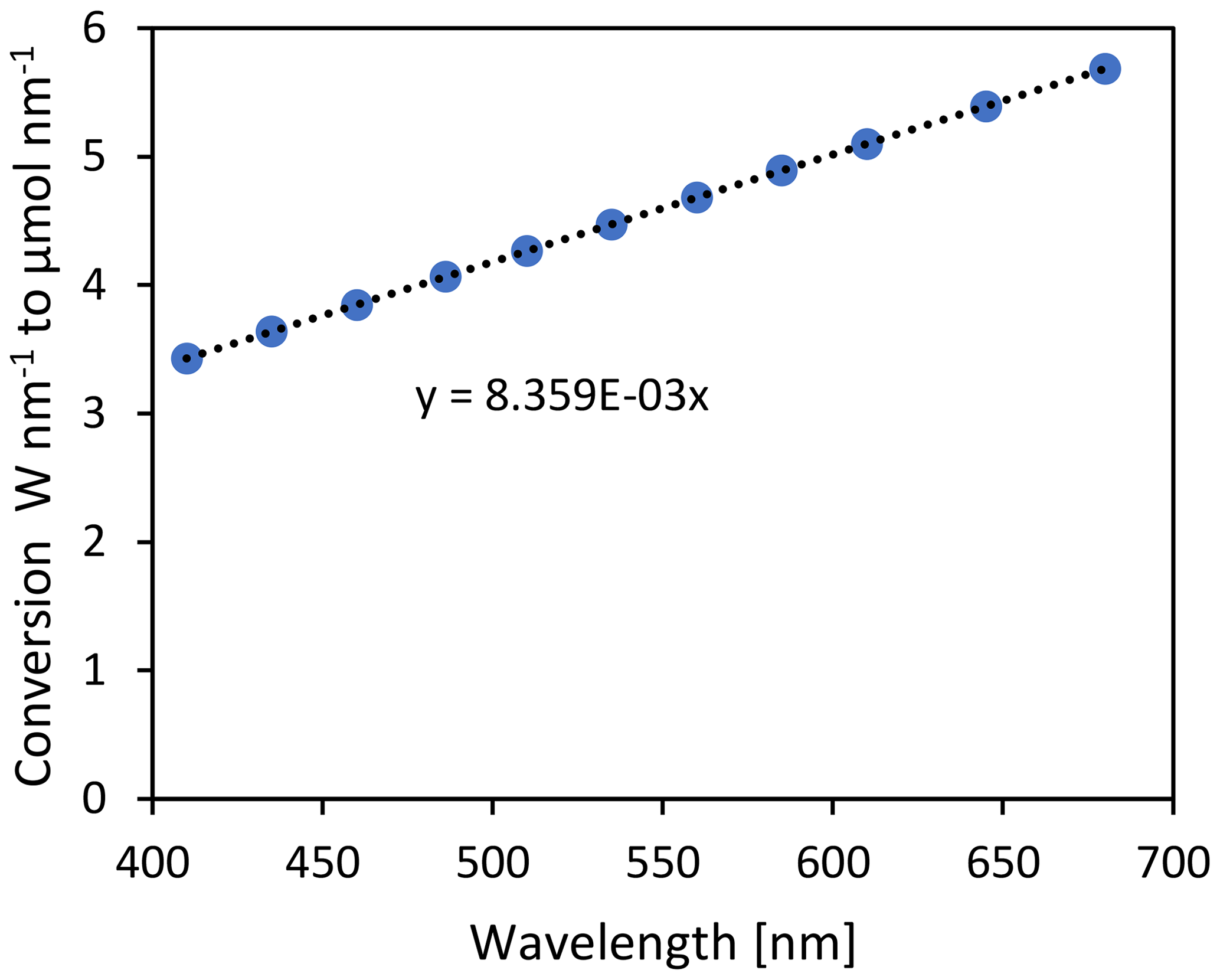
Note that the 11 channels within the PPFD range of FROST3 can be used to study vegetation-specific photosynthesis spectral response.

3.6 Vegetation development

FROST was tested during a field experiment in La Cendrosa, Spain (lat 41.692537^∘, long 0.931540^∘) (LIAISE campaign; Boone et al., 2021), from 14–22 July 2021. The instrument was placed on the bare soil surface at the moment the alfalfa vegetation started to develop. The normalized difference vegetation index (NDVI) (NIR − VIS) $/$ (NIR + VIS) is used in remote sensing to quantify crop growth; a low value is bare soil and a value of 1 represents a fully grown crop. It can be computed from at least two wavebands, one in the near infrared (> 700 nm) and a second waveband in the visible range. The two wavebands of 680 and 730 nm in version 1 are not affected by infrared crosstalk, and both measure at the same sensor chip to assure that both channels have the same viewing angle. Figure 22 shows daily values of NDVI.

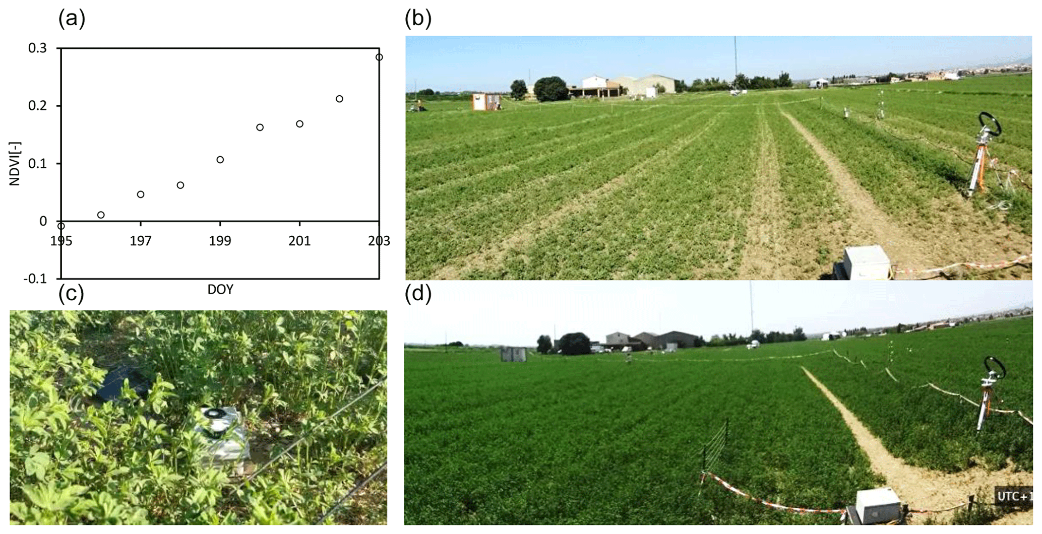
Figure 22 NDVI measurements calculated from FROST1 (with 10 mm diffuser) 680 and 730 nm wavebands located inside an alfalfa canopy. (c) FROST (top at about 8 cm height) placed on the surface in between alfalfa, crop height 30 cm (18 July). (b) Alfalfa crop on 14 July (crop height 23 cm). (d) Alfalfa crop (height 48 cm) on 22 July. Spain from 14–22 July 2022.

3.7 Surface albedo

A good test for the quality of the spectral measurements without having to deal with absolute calibration uncertainties comprises surface reflectance measurements. The typical spectral reflectance signature of healthy vegetation has two minima in the visible range at 500 and 675 nm and a small peak at 550 nm. Beyond 750 nm it is strongly reflective (about 50 %). A bare soil surface, in this case a sandy soil patch from a very deep soil layer that surfaced during the recent drilling of a well at the weather station, served as a bare soil plot and had a negligible organic soil fraction. The ASD FieldSpec was equipped with a cosine collector and operated in irradiance mode. Weather conditions were sunny with low soil moisture content of the bare soil. The comparison is good considering the difficulty of sampling the same spot for both instruments due to differences in the cosine response, size of sensor head, and leveling (Fig. 23).

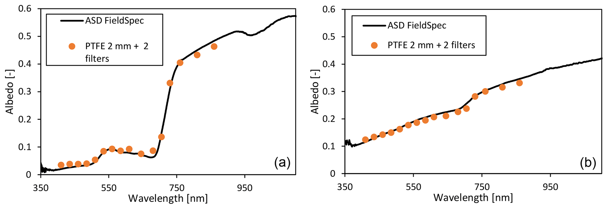
Figure 23 Spectral reflectance as measured by FROST3 and the ASD FieldSpec with cosine collector. (a) Spectral reflectance of grassland, Veenkampen weather station, 14:12 UTC on 15 May 2022; (b) sandy soil (dry, no organic fraction), 14:06 UTC on 15 May 2022.

The small underestimation of the 810 and 860 nm channels is related to the small cross-correlation with smaller wavelengths (Fig. 7, middle panels, and Fig. 23).

4 Concluding remarks

The FROST instrument will enable new research opportunities. It is much faster than traditional thermopile pyranometers and the low cost enables the deployment of large sensor grids. It can be deployed very quickly because it is a fully standalone, “plug and play” solution and measurements are always fully synchronized to UTC within at least 1 µs. The instrument has superior linearity (< 0.2 %), and the temperature coefficient is very low (−250 ppm K⁻¹) and was consistent among the three tested instruments. In contrast to thermopile sensors, FROST has no zero-offset errors. The drift with time appeared insignificant during a 2.5-month field test. Compared to PAR sensors, FROST can resolve the PAR spectra in 11 narrow wavebands (FWHM: 20 nm). This makes it possible to study wavelength-dependent photosynthesis responses of, for example, chlorophyll a and b. This is also relevant in canopy profile studies where solar irradiance extinction through a canopy modifies its light spectra. The fast response makes it possible to investigate the impact of the growth and wind-induced movements of vegetation on radiation fluctuations.

FROST measures GHI in 18 wavebands and includes a water absorption band, which makes it possible to derive information about atmospheric moisture such as column water vapor. Additionally, by using proper infrared crosstalk correction filters, it can monitor the spectral reflection properties of a surface with its first 16 wavebands from 410 to 860 nm. FROST can also be used to monitor vegetation growth by measuring NDVI.

We hope that other researchers will benefit from our crosstalk problem solution. Tran and Fukazawa (2020) used the same AMS spectroscopy sensor to determine optical properties of fruit, but they did not use LED light sources as recommended by the manufacturer. Their halogen light source emits much infrared light > 1000 nm, and therefore the six channels of their blue sensor and two of their six red sensor channels were greatly affected by infrared crosstalk. This is something they may not have been aware of because the AMS spectroscopy sensor datasheet does not show the filter response above 1000 nm. We believe their instrument performance would improve using our proposed correction filters.

Although the proposed cosine correction appears to give good results (2.5 W m⁻² standard error for daily averaged GHI), we will continue to improve the cosine collector for large zenith angles. PTFE as a diffuser material has better transmission properties below 400 nm than opal cast acrylic sheet glass, but it exhibits a 2 % stepwise increase in transmission beyond 21 ^∘C. Since the shortest waveband sensitivity of the FROST sensor is limited to 400 nm (considering FWHM), we recommend using opal cast acrylic glass diffusers for future versions. This would also remove UV radiation exposure and reduce sensor aging.