Extended validation of Aeolus winds with wind-profiling radars in Antarctica and Arctic Sweden

Winds from two wind-profiling radars, ESRAD (ESrange atmospheric RADar) in Arctic Sweden and MARA (Moveable Atmospheric Radar for Antarctica) on the coast of Antarctica, are compared with collocated (within 100 km) winds measured by the Doppler lidar on board the Aeolus satellite for the time period July 2019–May 2021 (baseline 2B11). Data are considered as a whole and subdivided into summer and winter as well as ascending (afternoon) and descending (morning) passes. Mean differences (bias) and random differences are categorized (standard deviation and scaled median absolute deviation) and the effects of different quality criteria applied to the data are assessed, including the introduction of the “modified Z score” to eliminate gross errors. This last criterion has a substantial effect on the standard deviation, particularly for Mie winds. Significant bias is found in two cases, for Rayleigh winds for the descending satellite passes. at MARA (−1.4 (+0.7) m s⁻¹) and for all Mie winds at ESRAD (+1.0 (+0.3) m s⁻¹). For the Rayleigh winds at MARA, there is no obvious explanation for the bias in the data distribution. The Mie wind error with respect to the wind data measured at ESRAD shows a skewed distribution toward positive values (Aeolus horizontal line-of-sight wind > ESRAD wind). Random differences (scaled median absolute deviation) for all data together are 5.9 and 5.3 m s⁻¹ for Rayleigh winds at MARA and ESRAD, respectively, and 4.9 and 3.9 m s⁻¹ for Mie winds. When the comparison is restricted to Aeolus measurements with a mean location within 25 km from the radars, there is no change to the random differences for Rayleigh winds, but for Mie winds they are reduced to 3.3 and 3.6 m s⁻¹. These represent an upper bound for Aeolus wind random errors since they are due to a combination of spatial differences and random errors in both radar winds and Aeolus winds. The random errors in radar winds are < 2 m s⁻¹ and therefore contribute little, but spatial variability clearly makes a significant contribution for Mie winds, especially at MARA.

1 Introduction

The Aeolus satellite mission is the first attempt to measure meteorological wind profiles on a global scale from space using the Doppler lidar technique. It carries a single instrument – the Atmospheric Laser Doppler Instrument (ALADIN) – which uses two detectors to measure backscattered laser light from cloud and aerosol particles (Mie scatter) and molecules (Rayleigh scatter), respectively (Stoffelen et al., 2005; ESA, 2008; Reitebuch, 2012). It was launched on 22 August 2018, and, from the planning stage, a wide range of validation tests were proposed, comparing the wind profiles from the satellite with those measured by established techniques such as radiosondes, ground-based radars, and lidars.

Validation exercises soon after the start of the mission found that the quality of retrieved winds in part depended on the satellite's geolocation and on orbit orientation (see e.g. Guo et al., 2021; Lux et al., 2021). This could be traced back to unexpected instrumental effects, most prominently the influence of temperature on the performance of the primary telescope mirror of the instrument (Witschas et al., 2020; Lux et al., 2021; Weiler et al., 2021). The subsequent changes to the data processing gave substantial improvement of the biases from more than 5 m s⁻¹ (Martin et al., 2021; Rennie and Isaksen, 2020) to less than 2 m s⁻¹ (e.g. Iwai et al., 2021; Baars et al., 2023). However, Baars et al. (2023) noted that those improvements were partly masked by worsening instrument performance (e.g. decrease in laser output energy) that led to an increase in the random error. Nevertheless, Aeolus winds have been shown to make a positive contribution to global weather forecasting (Reitebuch et al., 2020; Rennie et al., 2021; Weiler et al., 2021). A good number of validation comparisons of the corrected data processing after 2020 against a variety of other data sources have been reported, such as radiosondes (e.g. Martin et al., 2021; Rani et al., 2022; Chou et al., 2022), wind-profiling radar (e.g. Guo et al., 2021; Kottayil et al., 2022; Chou et al., 2022), Doppler wind lidars (e.g. Chen et al., 2022; Witschas et al., 2022), numerical weather prediction models (e.g. Lux et al., 2022; Rani et al., 2022), and other satellites (Lukens et al., 2022). Overviews of recent validation comparisons were summarized by e.g. Wu et al. (2022) and Ratynski et al. (2023), which mostly indicate possible biases less than 1 m s⁻¹ and random errors 4–7 m s⁻¹ for Rayleigh winds and 2–4 m s⁻¹ for Mie winds. At the same time, the biases and random errors seem to vary more than might be expected between the different measurement techniques and locations used in the validations. Lux et al. (2022) have looked in detail at the non-random nature of differences between Aeolus winds and reference winds and suggest that the exact details of quality control applied in validation studies can significantly affect the results. They found that the bias and random error estimates can be affected by small numbers of outliers, particularly for Mie winds where large errors outside a Gaussian distribution (gross errors) can be caused by misinterpretation of noise as signal. This can lead to predominantly positively biased gross errors.

An initial validation comparing measurements from two wind-profiler radars in Arctic Sweden and in Antarctica, with Aeolus winds processed with the 2B10 baseline, was published by Belova et al. (2021a). This found biases < 2 m s⁻¹ and standard deviation of the differences between satellite and radar winds in the range 4–7 m s⁻¹. Note that a large bias first reported for Mie winds in the data for Antarctica was found to be in error as detailed in the corrigendum published in May 2022 (Belova et al., 2021a, Corrigendum). However, the available time period for comparison was short (only 6 months) and uncertainties in the biases were large. Almost 2 years of data from these high-latitude radars are now available for comparison with the longest available consistently processed Aeolus dataset (baseline 2B11) from July 2019 to May 2021. A comparison of these extended datasets, together with more detailed consideration of the statistics as suggested by Lux et al. (2022), is presented here.

2 Overview of measurements and quality criteria

The radars used are MARA (Moveable Atmospheric Radar for Antarctica), situated at Maitri in Antarctica (70.77^∘ S, 11.73^∘ E) and ESRAD (ESrange atmospheric RADar), situated near Kiruna in Arctic Sweden (67.88^∘ N, 21.10^∘ E). Full details of the radar and satellite operation modes as well as the available data can be found in Belova et al. (2021a, b). Each radar measures profiles of vertical and horizontal wind components in the vertical direction above the radar site. They switch automatically every 1–2 min between different modes with vertical resolutions of 75, 150, and 600 m (MARA) as well as 900 m (ESRAD). The radars sample a cone of the atmosphere with a width of about 5^∘ for ESRAD and 10^∘ for MARA, so the horizontal diameter of the radar beams in the lowest 10 km of the atmosphere is less than 2 km at MARA and 1 km at ESRAD. Random errors (standard deviation of all 1 or 2 min estimates in the 1 h averages) are typically 2–3 m s⁻¹ for both radars (Belova et al., 2021b). Comparison with radiosondes (Belova et al., 2021b) has shown no significant bias (< 0.25 m s⁻¹) for winds at MARA but systematic biases at ESRAD of 8 % for zonal winds and 25 % for meridional winds (ESRAD underestimates wind components). These are thought to be due to the geometry of the radar antenna field and a high level of local radio noise. The ESRAD wind estimates are corrected for these biases before being compared with Aeolus winds. For the comparison with Aeolus (as in Belova et al., 2021a), we use 1 h averaged winds, also averaged over the height intervals corresponding to the Aeolus Rayleigh wind averages. We use only radar measurements where the 95 % confidence limit of the 1 h mean is less than 2 m s⁻¹ (this is calculated from the standard deviation and the number of the samples in the 1 h average using Student's t test).

We select all satellite measurement tracks passing within 100 km from each radar site. For Aeolus Rayleigh (clear) winds, we then select the profile with the mean position closest to the radar (which is averaged over about 87 km along the track). For Aeolus Mie (cloudy) winds, which are averaged over about 14 km of track, we collect all observations within 100 km of the radar and average them within the same height bins as the corresponding Rayleigh profile. We use the horizontal line-of-sight (HLOS) winds from the Level 2B data product, here using the 2B11 baseline (ESA, 2023). Radar measurements of the full wind vector are averaged from 30 min before the pass to 30 min after the pass, again to the same height bins as the Rayleigh wind profile. Radar HLOS winds are calculated from the radar vector winds (ignoring the vertical component, which is found to be negligible in the 1 h averages). There are usually four Aeolus passes per week providing comparative data at MARA and three passes per week at ESRAD.

For the analysis in Belova et al. (2021a) only winds less than 100 m s⁻¹ (radar and Aeolus) with a validity flag of 1 (Aeolus) and with estimated error (EE, also included in the Aeolus Level 2B product) < 8 m s⁻¹ (Rayleigh), EE < 5 m s⁻¹ (Mie), and 95 % confidence limit < 2 m s⁻¹ (radar) were used. Here, as suggested by Lux et al. (2022), we first examine the statistics of the differences between radar and Aeolus winds for different quality criteria (QC). Differences are parameterized in terms of bias, standard deviation (SD), and scaled median absolute deviation (ScMAD), where

$$\begin{array}{}\text{(1)}& \mathrm{bias}={\displaystyle \frac{\mathrm{1}}{N}}\cdot {\sum }_{i=\mathrm{1}}^N\left({\mathrm{HLOS}}_{\mathrm{Aeolus},\mathrm{i}}-{\mathrm{HLOS}}_{\mathrm{radar},\mathrm{i}}\right),\end{array}$$

$$\begin{array}{}\text{(2)}& \mathrm{SD}=\sqrt{{\displaystyle \frac{\mathrm{1}}{N-\mathrm{1}}}\sum {\left(\left({\mathrm{HLOS}}_{\mathrm{Aeolus},\mathrm{i}}-{\mathrm{HLOS}}_{\mathrm{radar},\mathrm{i}}\right)-\mathrm{bias}\right)}^{\mathrm{2}}},\end{array}$$

$$\begin{array}{}\text{(3)}& \begin{array}{rl}& \mathrm{ScMAD}=\mathrm{1.4826}\cdot \mathrm{median}\left(\left|\left({\mathrm{HLOS}}_{\mathrm{Aeolus},\mathrm{i}}\right.\right.\right.\\ & \left.-{\mathrm{HLOS}}_{\mathrm{radar},\mathrm{i}}\right)\left.\left.-\mathrm{median}\left({\mathrm{HLOS}}_{\mathrm{Aeolus},\mathrm{i}}-{\mathrm{HLOS}}_{\mathrm{radar},\mathrm{i}}\right)\right|\right).\end{array}\end{array}$$

Both SD and ScMAD are estimates of the variability of the wind error, but ScMAD is less susceptible to outliers. If the distribution is Gaussian, they have the same value.

In order to determine suitable QC, we first look at these parameters as a function of EE threshold for Rayleigh and Mie winds and with and without a second quality criterion, designed to eliminate gross errors, based on the modified Z score (ModZ) (Iglewicz and Haglin, 1993), as suggested by Lux et al. (2022):

$$\begin{array}{}\text{(4)}& {\mathrm{ModZ}}_i={\displaystyle \frac{\begin{array}{c}\left|\left({\mathrm{HLOS}}_{\mathrm{Aeolus},\mathrm{i}}-{\mathrm{HLOS}}_{\mathrm{radar},\mathrm{i}}\right)\right.\\ \left.-\mathrm{median}\left({\mathrm{HLOS}}_{\mathrm{Aeolus},\mathrm{i}}-{\mathrm{HLOS}}_{\mathrm{radar},\mathrm{i}}\right)\right|\end{array}}{\begin{array}{c}\mathrm{ScMAD}\\ \end{array}}}.\end{array}$$

Figure 1 shows the fraction of possible comparison points (n) retained, biases, SD, and ScMAD as a function of the EE threshold used for rejection at MARA. Parameters with the subscript z (n_z, bias_z, SD_z, ScMAD_z) have been calculated after further rejecting data points with ModZ_i > 3.5. Values for this limit between 3.0 and 3.5 were found to lead to a high degree of normality for differences between Aeolus observations and ECMWF background winds by Lux et al. (2022). We have also tested rejecting ModZ_i > 3.0, but the differences are very small so we show only results using ModZ_i > 3.5.

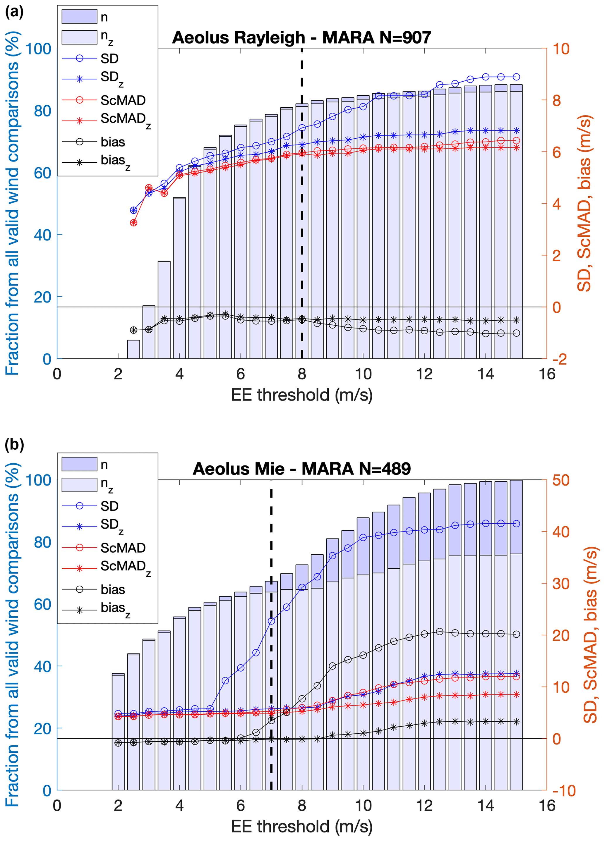
Figure 1 Comparison of Aeolus HLOS winds with MARA (for all available data) (a) for Rayleigh-clear winds and (b) for Mie-cloudy winds. Plots show the fraction of possible comparison points (n) retained, biases, SD, and ScMAD as a function of the EE threshold used for rejection. The subscript z (n_z, bias_z, SD_z, ScMAD_z) shows results after further rejecting data points with ModZ > 3.5. N in the panel titles is the number of samples corresponding to n = 100 %. The vertical dashed line marks the EE threshold used for the analysis in the rest of the paper.

In Fig. 1, for Rayleigh winds it is clear that SD rises steeply for EE > 7 m s⁻¹, but this is much less apparent where the check on ModZ_i has removed outliers (SD_z). ScMAD is insensitive to the ModZ_i restriction and is close to SD_z up to 8 m s⁻¹, suggesting a close to Gaussian distribution after the ModZ_i restriction. Bias and bias_z are consistently small (about −0.5 m s⁻¹) from EE > 3.5 m s⁻¹ up to 8 m s⁻¹, and bias_z remains at this level for all EE thresholds tested. Thus, the original choice of EE < 8 m s⁻¹ as the QC for Rayleigh winds seems reasonable. For Mie winds at MARA, both SD and bias increase sharply for EE > 5 m s⁻¹. ScMAD_z and SD_z remain very close to each other up to EE < 8.5 m s⁻¹. Bias_z remains small and at a rather constant level from EE < 5 to EE < 8.5 m s⁻¹. The fraction of total comparison points left after applying both the EE and ModZ_i rejection criteria (n_z) increases sharply for EE < 5 m s⁻¹ and more slowly after that to just over 80 % for Rayleigh (corresponding to ∼ 800 points) and to about 70 % for Mie winds (∼ 350 points). So, in order to include as many points as possible and a distribution as close as possible to Gaussian, it seems reasonable to increase the original threshold of EE < 5 m s⁻¹ for Mie winds to anywhere up to EE < 8 m s⁻¹ together with the outlier rejection using ModZ_i < 3.5.

Figure 2 shows corresponding plots at ESRAD. For Rayleigh winds, the bias and bias_z are insensitive to the EE threshold from EE < 5 m s⁻¹ to EE < 15 m s⁻¹. SD increases sharply at EE < 10 m s⁻¹ and above. Otherwise, SD_z, ScMAD, ScMAD_z, and the difference between SD_z and ScMAD_z all increase slowly but steadily for all EE thresholds above EE < 5 m s⁻¹. Thus, there is no clear motivation for a particular choice of EE threshold for Rayleigh winds. For Mie winds at ESRAD, SD and bias increase rapidly with EE thresholds > 5 m s⁻¹, while SD_z, ScMAD, ScMAD_z, and the difference between SD_z and ScMAD_z seem to increase more rapidly for EE threshold > 7.0 m s⁻¹. The bias_z increases slowly across all EE thresholds but is fairly constant between EE < 5 m s⁻¹ and EE < 7 m s⁻¹. The fraction of total comparison points left after applying both the EE and ModZ_i rejection criteria (n_z) increases sharply for EE < 5 m s⁻¹ and more slowly after that to just over 90 % for Rayleigh (corresponding to ∼ 1800 points) and to about 70 % for Mie winds (∼ 700 points).

Figure 2 As Fig. 1 but for ESRAD.

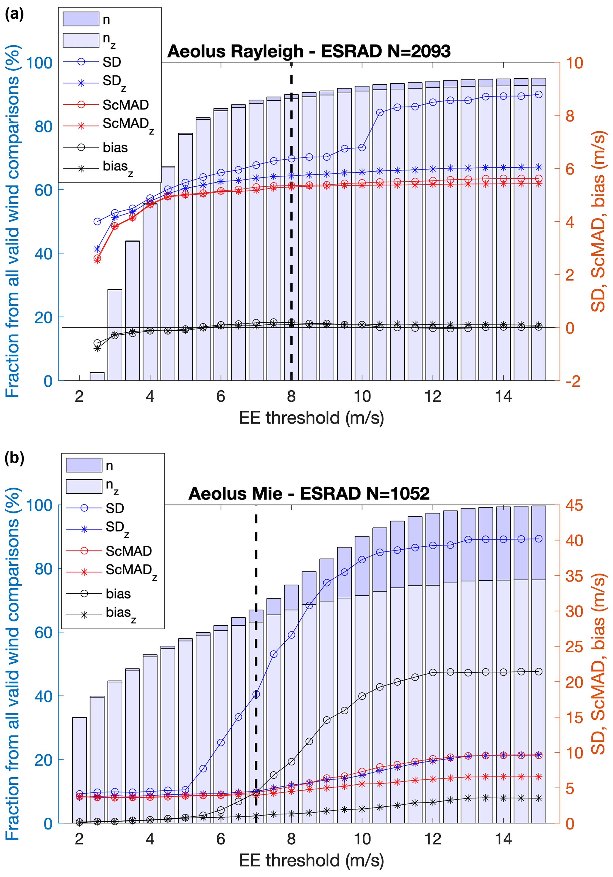
Figures 1 and 2 show very similar behaviour at MARA and at ESRAD, so there is no obvious reason to treat the data from the two sites differently. We have made similar plots for all of the data subsets, which we analyse below and found no reason to choose different thresholds for the different subsets. In all cases, ScMAD is close to ScMAD_z, and their values are constant or changing very slowly for EE values 1 m s⁻¹ above or below the thresholds. Similarly, bias and bias_z are close together and insensitive to the EE values around the chosen thresholds, although both the bias_z and ScMAD_z values can lie at different levels in the different subsets, as shown in Tables 1 and 2 and discussed in the next section. Thus, in the following we adopt QC using only Aeolus winds with estimated random error (EE) < 8 m s⁻¹ (Rayleigh) and < 7 m s⁻¹ (Mie), rejecting likely gross errors where ModZ > 3.5. This results in 80 %–90 % of Rayleigh wind comparison points and about 60 % of Mie wind points being available for analysis, which are sufficient numbers for further division according to summer–winter and ascending–descending orbits. The same restrictions on radar winds as in Belova et al. (2021a) are also applied – wind speed less than 100 m s⁻¹ and 95 % confidence limit < 2 m s⁻¹.

Table 1 Statistics of correlation and differences between Aeolus Rayleigh-clear HLOS winds and MARA HLOS winds. $\left|u_{\mathrm{HOS}}\right|$ shows the median Aeolus HLOS wind speed in each data subset, with the values between square brackets corresponding to the lower and upper quartiles of the distribution. N_z is the number of comparison points passing all quality checks (QC; see text for details); the percent of outliers is the number of points rejected by the final QC (ModZ < 3.5, Eq. 4). Slope_z is the slope of the best-fit straight-line correlation, and bias_z, SD_z, and ScMAD_z are as defined in Eqs. (1)–(3). Columns are for all data (July 2019–May 2021) or divided into summer (23 September–22 March), winter (23 March–22 September), descending, and ascending passes. For slope_z and bias_z, values between square brackets are 95 % confidence limits. Rayleigh winds with EE > 8 m s⁻¹ are excluded.

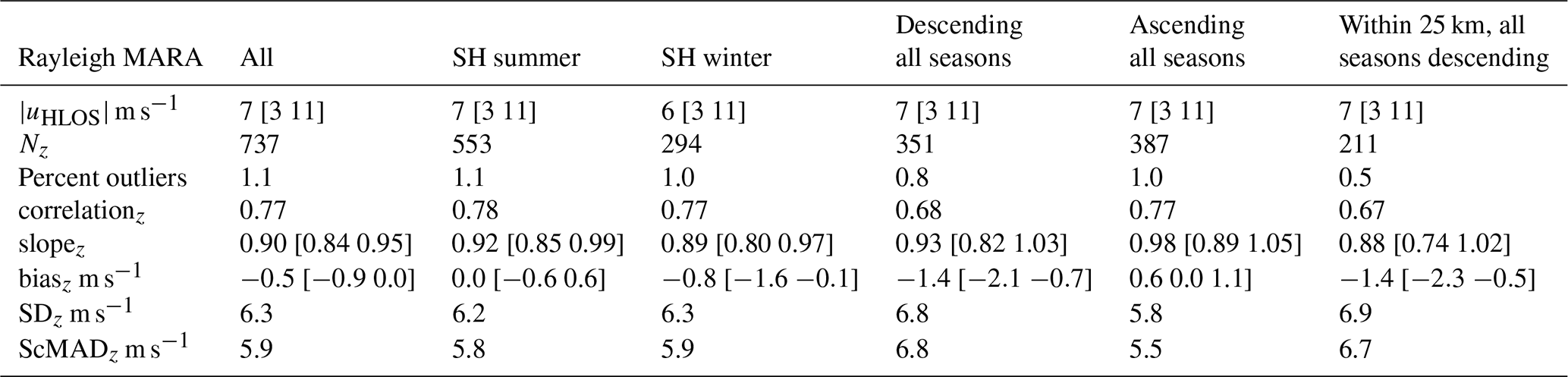
Table 2 As Table 1, but for Aeolus Mie-cloudy HLOS winds and MARA HLOS winds. Mie winds with EE > 7 m s⁻¹ are excluded.

3 Comparison with MARA, Antarctica

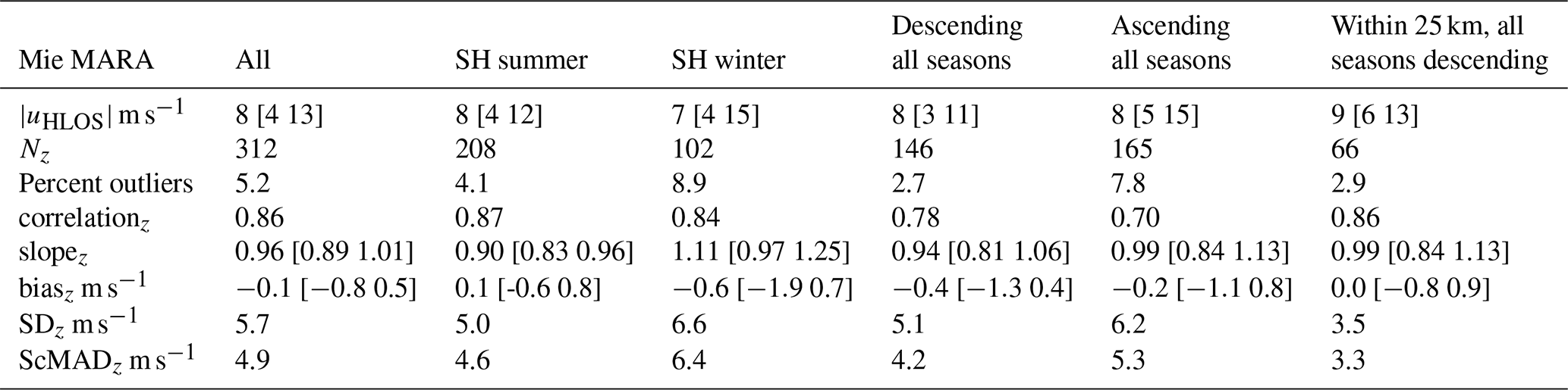
Statistics of the comparison between Aeolus and MARA are given in Table 1 (Rayleigh winds) and Table 2 (Mie winds), and scatter plots of the comparisons are shown in Fig. 3 (note that no correction is made in the tables for the random uncertainties in radar measurements). The first column in each table shows the comparison for all of the data, corresponding to Fig. 1 at EE thresholds 8 m s⁻¹ for Rayleigh winds and 7 m s⁻¹ for Mie winds. The tables also show the results after dividing the data by season (summer, 23 September–22 March; winter, 23 March–22 September) and by ascending (afternoon) and descending (morning) Aeolus passes. Variations of, for example, solar illumination on the ground between summer and winter as well as opposite lidar backscatter direction relative to the prevailing wind between ascending and descending passes could in principle affect the comparison. Seasonal influences on the instrument performance have also been found to be important, particularly for the bias (Weiler et al., 2021). Tables 1 and 2 also include a further column which shows the results when the comparison is restricted to Aeolus measurements within 25 km of MARA (more precisely, those with the mid-point of the average along the orbit track within 25 km). Because of the geometry of the satellite orbit, these are all on descending passes. Note that since Rayleigh winds are averaged over about 87 km distance along the track, those measurements will still include observations up to 68 km from the radar along the track. For Mie winds, which are averaged over 15 km, observations up to 33 km away can contribute.

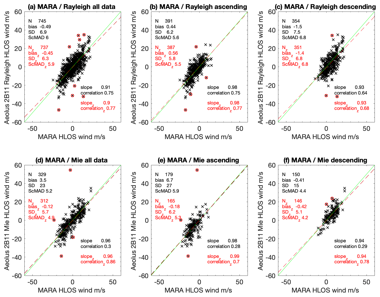
Figure 3 Scatter plots of Aeolus HLOS Rayleigh-clear winds (a–c) and Mie-cloudy winds (d–f) vs. MARA winds. Panels (a, d) show all orbits together, panels (b, e) show ascending passes, and panels (c, f) show descending passes. Red circles show data points removed by the ModZ > 3.5 QC. Parameters in black and red indicate fits including and excluding these points, respectively. The green line is where the Aeolus wind is exactly equal to the MARA wind. Units for bias_z, SD_z, and ScMAD_z are metres per second (m s⁻¹).

For the Rayleigh winds, Table 1 shows that there are no significant differences between summer and winter (note that results restricted to Aeolus measurements within 25 km from the radar are shown only in the tables; all of the figures include points up to 100 km from the radar). There does seem to be a significant difference between ascending and descending passes, with descending passes showing lower correlation, stronger (negative) bias, and higher SD_z and ScMAD_z. These differences can also be discerned by comparing Fig. 3b and c. For all of the data together, there is a small, marginally significant bias. As can be seen in Fig. 1, this bias is largely independent of the choice of EE threshold for data rejection.

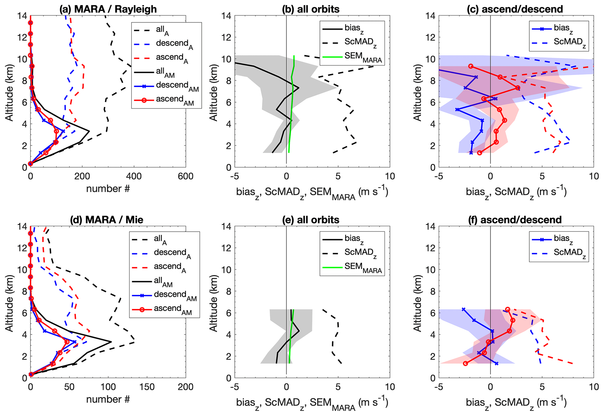
Figure 4 Comparison of Aeolus winds with MARA. Panels (a, d) show height profiles of numbers of data points, and dashed lines with the subscript A show the number of Aeolus wind observations with EE > 8 m s⁻¹ (Rayleigh) or 7 m s⁻¹ (Mie). Solid lines with the subscript AM show the number of points included in the analysis, i.e. where MARA data are also available and modZ < 3.5. Panels (b, e) show height profiles of the mean values of the uncertainty in MARA wind estimates (green line, SEM_MARA), bias_z, and ScMAD_z for all orbits together. Panels (c, f) show bias_z and ScMAD_z separately for ascending and descending passes.

For the Mie winds, Table 1 shows that there are (in %) twice as many outliers rejected by the ModZ < 3.5 QC in winter compared to summer. SD_z and ScMAD_z are also higher in winter, but the biases are not significantly different. Ascending passes show a higher rate of outliers and higher SD_z and ScMAD_z compared to descending, but again with no significant bias for either. Again the differences can be discerned by comparing Fig. 3e and f. The differences in variability between ascending and descending passes are opposite for Mie winds compared to Rayleigh winds; the differences in variability between summer and winter affect only the Mie winds and significant bias for the descending passes affects only the Rayleigh winds, so they are unlikely to be explained by meteorology or by systematic errors in radar wind speed. Overall, SD_z and ScMAD_z are slightly higher for Rayleigh winds (around 6 m s⁻¹) than for Mie winds (around 5 m s⁻¹). Comparing the red and black numbers in Fig. 3 also shows the large change in SD and bias for Mie winds when the ModZ < 3.5 quality criterion is applied (comparing bias and SD with bias_z and SD_z, respectively).

Figure 5 As Fig. 3 but for ESRAD.

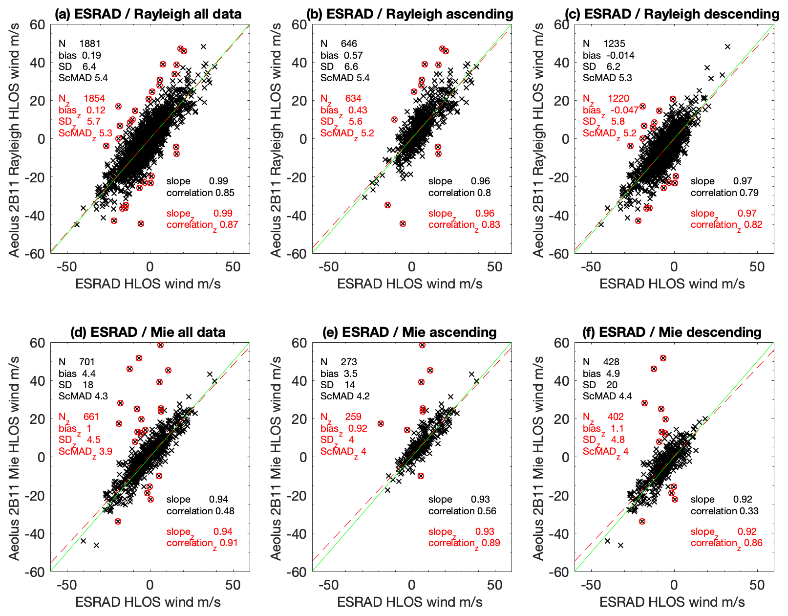
Figure 4 shows height-resolved parameters for the Aeolus–MARA comparison. Figure 4a and d show that low heights between 1 and 5 km dominate the comparison even though Aeolus wind estimates are available throughout the troposphere (and higher in the case of Rayleigh winds). This is due to the low sensitivity of the MARA radar in the upper troposphere and above. The uncertainty in radar winds is shown by the green line in Fig. 4b and c. Each radar wind is estimated from a 1 h average of measurements, and the standard error of the mean (SEM) is used as an estimate of the uncertainty. Since we include only averaged radar winds where the 95 % confidence interval is < 2 m s⁻¹ (this is twice the SEM when the number of data points in the average is large), SEM is low (below 1 m s⁻¹) and increases only slightly with height. (The SEM_MARA profile is essentially the same for the ascending and descending passes as for all data, so, for clarity, it is not included in the plot.) In Fig. 4e and f we can see that the negative bias for Rayleigh descending winds, seen in Tables 1 and 2, is seen at almost all heights, although the uncertainties in the bias become very large above 6 km height. It is partly balanced by a positive bias (marginally significant) for the ascending passes so that, for all data together (Fig. 4b and e), the mean bias becomes closer to zero. For the Mie winds, with notably more restricted height coverage, there is no significant bias at any height.

4 Comparison with ESRAD, Arctic Sweden

Tables 3 (Rayleigh winds) and 4 (Mie winds) show statistics of the comparison between Aeolus and ESRAD. Scatter plots of the comparisons are shown in Fig. 5. The comparison for all of the data is shown in the first column in each table, corresponding to Fig. 2 at EE thresholds 8 m s⁻¹ for Rayleigh winds and 7 m s⁻¹ for Mie winds. The tables also show the results after dividing the data by season (winter, 23 September–22 March; summer, 23 March–22 September) and by ascending (afternoon) and descending (morning) Aeolus passes. The final column in Tables 3 and 4 shows the results when the comparison is restricted to Aeolus measurements with their mid-points within 25 km of ESRAD. These are all on ascending passes and, due to averaging, will include observations up to 68 km and 33 km from the radar along the track for Rayleigh and Mie winds, respectively.

Table 3 Statistics of correlation and differences between Aeolus Rayleigh-clear HLOS winds and ESRAD HLOS winds. $\left|u_{\mathrm{HLOS}}\right|$ shows the median Aeolus HLOS wind speed in each data subset, with the values between square brackets corresponding to the lower and upper quartiles of the distribution. N_z is the number of comparison points passing all quality checks (QC; see text for details); the percent of outliers is the number of points rejected by the final QC (ModZ < 3.5, Eq. 4). Slope_z is the slope of the best-fit straight-line correlation, and bias_z, SD_z, and ScMAD_z are as defined in Eqs. (1)–(3). Units for bias_z, SD_z, and ScMAD_z are metres per second (m s⁻¹). Columns are for all data (July 2019–May 2021) or divided into summer (23 March–22 September), winter (23 September–22 March), descending, and ascending passes. For slope_z and bias_z, values between square brackets are 95 % confidence limits. Rayleigh winds with EE > 8 m s⁻¹ are excluded.

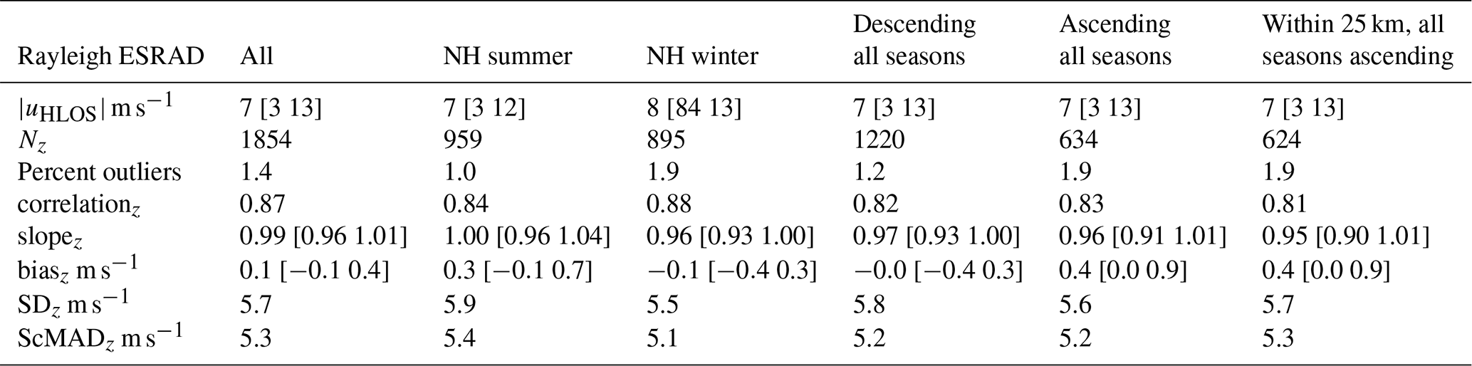
Table 4 As Table 3, but for Aeolus Mie-cloudy HLOS winds and ESRAD HLOS winds. Mie winds with EE > 7 m s⁻¹ are excluded.

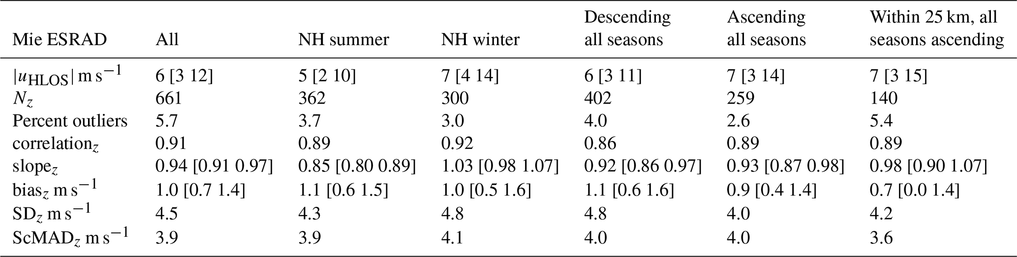
In Table 3 (Rayleigh winds), there are no significant differences between summer and winter or between ascending and descending passes, and bias_z in all cases is not significantly different from zero. In Table 4 (Mie winds), there are again no significant differences between summer and winter or between ascending and descending passes. However, there is a significant bias of about 1 m s⁻¹ for all cases. Overall, SD_z and ScMAD_z are slightly higher for Rayleigh winds (around 5 m s⁻¹) than for Mie winds (around 4 m s⁻¹) and slightly lower than at MARA.

Figure 5 illustrates the distribution of points about the regression lines and shows how the rejection of points with ModZ > 3.5 has effectively eliminated several gross errors. Figure 5 (comparing the black numbers for bias and SD with the red numbers for bias_z and SD_z) also shows the large change in SD and bias for Mie winds when the ModZ < 3.5 quality criterion is applied.

Figure 6 provides height-resolved profiles of parameters for the Aeolus–ESRAD comparison. As can be seen in Fig. 5a and d, in contrast to MARA, the more powerful ESRAD provides useful coverage in the upper troposphere as well as the lower troposphere. There are fewer joint ESRAD–Aeolus observations than Aeolus alone. Between 2 and 5 km height almost all Aeolus measurements (from this height range) have corresponding radar measurements. Higher up in the troposphere, about half of the Aeolus measurements (from this height range) have corresponding radar measurements. The green line in Fig. 5b and e shows the mean SEM for the ESRAD wind averages. Numbers can be as high as 1 m s⁻¹ in the upper troposphere but are lower at lower heights. (The SEM_ESRAD profile is essentially the same for the ascending and descending passes as for all data, so, for clarity, it is not included in the plot.) Considering the bias profiles in Fig. 4b, c, e, and f, above 6 km height, the bias uncertainties are notably lower than at MARA – this is a result of a much larger number of comparison points thanks to the higher power of ESRAD. For Rayleigh winds there is no significant bias at any height, and for Mie winds the ∼ 1 m s⁻¹ positive bias identified in Table 4 is clearly seen at all heights. From Fig. 2 it is clear that a positive bias appears whatever the EE threshold.

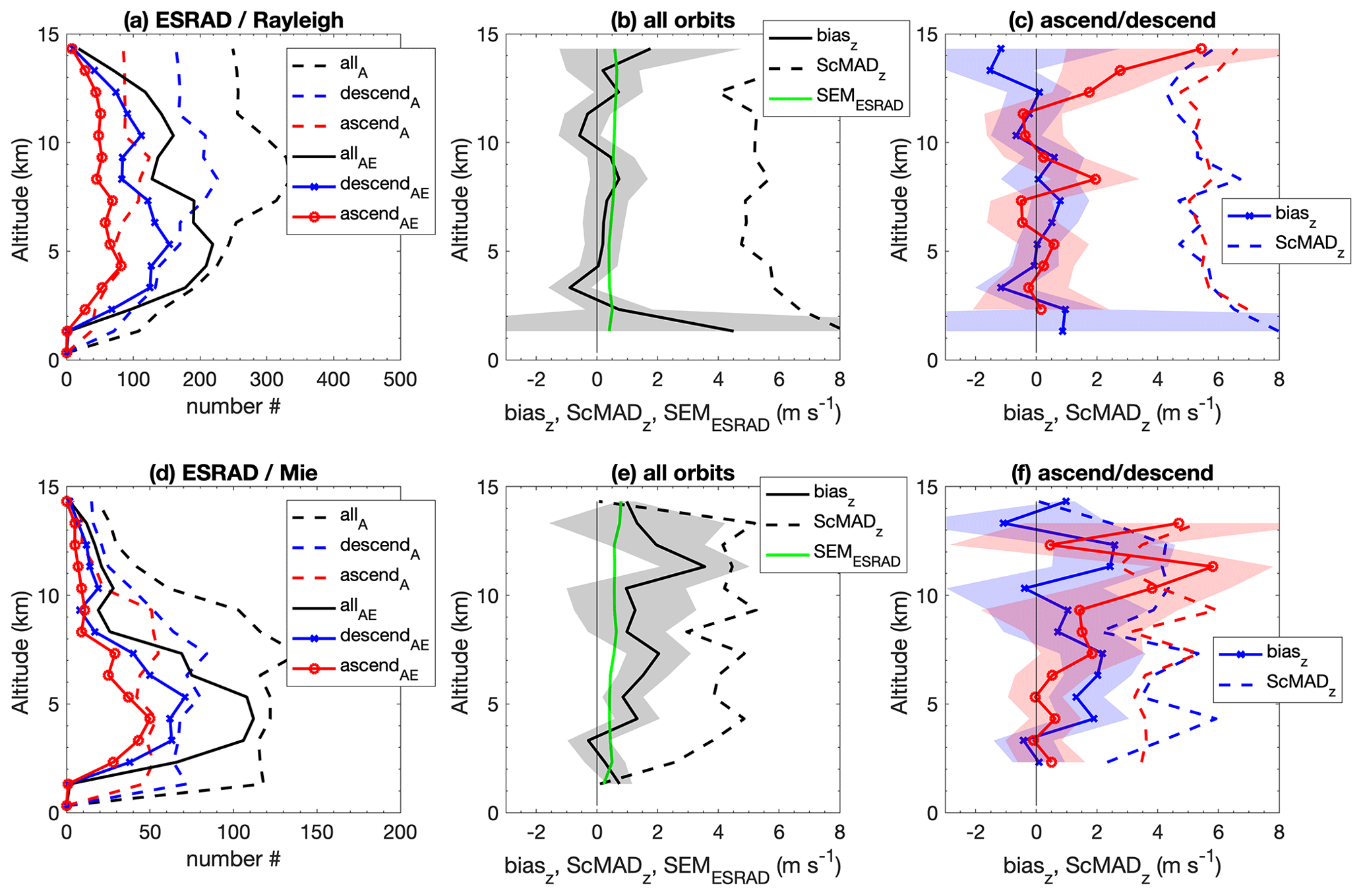
Figure 6 Comparison of Aeolus winds with ESRAD. Panels (a, d) show height profiles of numbers of data points, and dashed lines with the subscript A show the number of Aeolus wind observations with EE > 8 m s⁻¹ (Rayleigh) or 7 m s⁻¹ (Mie). Solid lines with the subscript AE show the number of points included in the analysis, i.e. where ESRAD data are also available and modZ < 3.5. Panels (b, e) show height profiles of the mean values of the uncertainty in ESRAD wind estimates (green line, SEM_ESRAD), bias_z, and ScMAD_z for all orbits together. Panels (c, f) show bias_z and ScMAD_z separately for ascending and descending passes.

5 Further analysis of non-zero biases

The analysis above has identified significant non-zero biases in two cases – for Rayleigh winds at MARA (descending passes, bias_z −1.4 m s⁻¹) and for all Mie winds at ESRAD (bias_z+1 m s⁻¹). To check these further, we plot normal probability curves for a series of EE thresholds in Figs. 7 and 8. These plots compare the distribution of the data (Aeolus HLOS wind–radar HLOS wind, after applying the ModZ < 3.5 QC) to the normal distribution (+). A reference line (red) joins the first and third quartiles of the data and is projected to the ends of the data. If the sample data have a normal distribution, then the data points appear along the reference line. Departures from the line to the right at the positive end and to the left at the negative end show “fat tails” (more points in the tails of the data distribution than in the normal distribution). When one tail is bigger than the other the distribution is skewed.

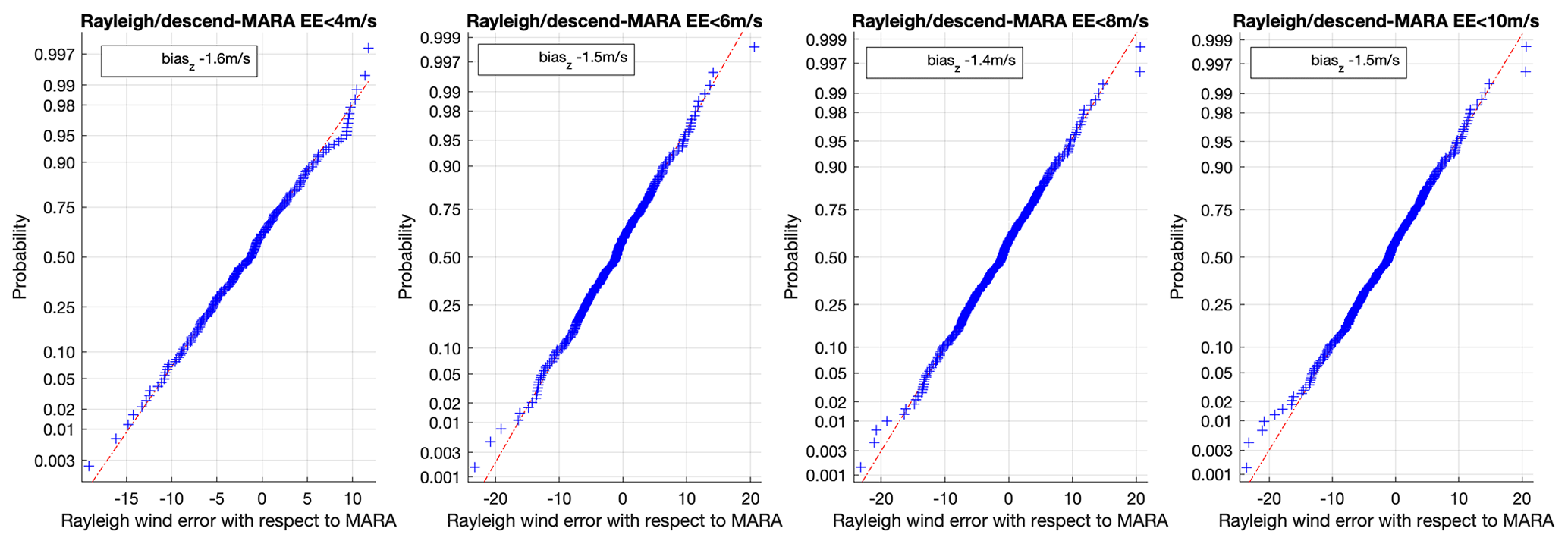
Figure 7 Normal probability plot for the difference between Aeolus Rayleigh HLOS wind and MARA wind (descending passes) for a series of EE thresholds, after rejecting points with ModZ > 3.5. See text for details.

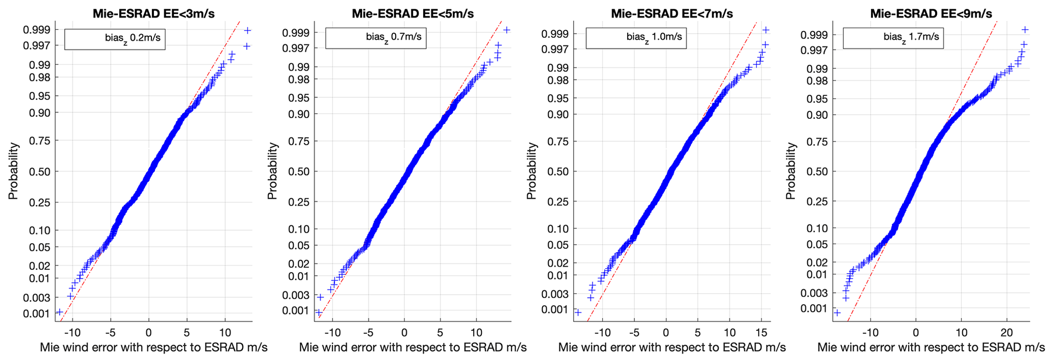
Figure 8 Normal probability plot for the difference between Aeolus Mie HLOS wind and ESRAD wind (all passes) for a series of EE thresholds, after rejecting points with ModZ > 3.5. See text for details.

Figure 7 (Rayleigh descending – MARA) shows fairly symmetric, small fat tails which grow slightly as the EE threshold is increased. The bias remains the same over the range of EE thresholds. This same constant bias over all EE thresholds can be seen for all of the Rayleigh MARA winds in Fig. 1. Figure 8 (Mie – ESRAD) shows small fairly symmetric fat tails for low values of the EE threshold, but these grow large and become skewed at the higher EE thresholds, leading to an increase in the bias estimate. This is also seen in Fig. 2. There is no obvious reason why the distribution is skewed only for Mie winds and only at ESRAD. One possibility might be local meteorology as the ESRAD area is often covered by mountain-lee-wave clouds which might affect Mie (cloudy) measurements differently than Rayleigh (clear) measurements. In general, vertical winds of up to 2 m s⁻¹ can be found in the troposphere in mountain lee waves at ESRAD (Kirkwood et al., 2010). However, the horizontal wavelengths of the lee waves are only a few tens of kilometres and would be averaged along the Aeolus track. In the comparison dataset here, 99 % of the data points have vertical winds within +0.4 and −0.4 m s⁻¹ at ESRAD, and there is no correlation between vertical wind and the difference between ESRAD and Aeolus HLOS winds. So vertical winds cannot explain the skewed distribution. Preferential locations for cloud formation within the wave wind field could affect Mie winds differently than Rayleigh winds. Extensive case studies would be needed to test this possibility.

6 Discussion and conclusions

In the present study we have compared 2 years of wind measurements by the Aeolus satellite (Rayleigh-clear and Mie-cloudy) with winds from two wind-profiler radars in Arctic Sweden and in coastal Antarctica, respectively. For each radar we have looked at ascending and descending passes and summer and winter separately, as well as for all of the data together. We have identified significant non-zero biases in only two subsets of the data – for Rayleigh winds at MARA (winter descending passes, bias −1.4 m s⁻¹) and for Mie winds (all passes) at ESRAD (bias +1 m s⁻¹). Biases for all other subsets are not different from zero at the 95 % confidence limits. In the initial validation of Aeolus winds against the MARA radar (Belova et al., 2021a) significant bias (−2 m s⁻¹) was also found for Rayleigh winds (descending passes) at MARA, which is similar to the result here. For Mie winds (Belova et al., 2021a, Corrigendum), the initial study also found a positive bias similar to the present study at ESRAD (average +1.2 m s⁻¹). The number of comparison points has increased by about a factor of 3 in the present study due the longer time period (2 years instead of 6 months), and, for Mie winds, the relaxation of the random error (EE) threshold for rejection of data increased from 5 to 7 m s⁻¹. With the increase in numbers and the introduction of a new criterion for rejection of outliers (modZ < 3.5), the uncertainties in the bias estimates have been substantially reduced (from 1–3 to 0.3–1 m s⁻¹) so we can be more confident that the estimated biases are accurate. It seems clear that uncorrected biases can still appear for our particular locations even after the data processing improvements incorporated in the L2B product with the 2B11 baseline. In addition, for Mie winds at ESRAD there is clearly a problem with a skewed distribution of random errors, with substantial numbers of Mie (HLOS) winds which are greater in magnitude than the radar winds, larger than expected for a normal distribution, and difficult to remove even with the new outlier constraint (modZ < 3.5). The problem of skewness for Mie winds has also been reported and addressed in detail by Lux et al. (2022).

The biases are similar in magnitude to results from other locations (e.g. Wu et al., 2022; Ratynski et al., 2023, and summaries included in those papers). Both Kottayil et al. (2022) and Ratynski et al. (2023) found no differences in the statistical results for ascending and descending passes. However, Martin et al. (2022) noted that biases can depend on latitude. It should be noted that Lukens et al. (2022) found large differences in the standard deviation of atmospheric motion vectors over Antarctica that were derived from Aeolus winds and from geostationary satellites and indicated that this is due to problems with the correct height assignment. Chou et al. (2022) presented a validation comparison with both radiosondes and radar in northern Canada, i.e. from latitudes similar to ESRAD. They found that Aeolus winds correlate well with their radiosonde data. On the other hand, correlation with radar winds was much less good. The reasons were twofold: firstly, the radar only operated for a limited time, leading to only a small number of profiles being available for comparison; secondly, the range of the radar was limited, as it was not optimized to measure winds but rather hydrometeors (e.g. rain).

Random differences (ScMAD_z) for all data together are 5.9 and 5.3 m s⁻¹ for Rayleigh winds at MARA and ESRAD, respectively, and 4.9 and 3.9 m s⁻¹ for Mie winds. We note that the random errors in the radar measurements should be < 2 m s⁻¹ (we have used only radar wind estimates where the 95 % confidence limit for the 1 h average is < 2 m s⁻¹) so that this should contribute little to the SD of the differences between radar and Aeolus measurements (less than 0.5 m s⁻¹ assuming uncorrelated random errors). Since Aeolus HLOS winds have been sampled within a few tens of kilometres from the radar sites, we can use the comparison of radar measurements with radiosondes by Belova et al. (2021a) to give some indication of the possible combined effects of spatial variability and random errors in the radar measurements (sondes, although launched at the radar sites, can be several tens of kilometres away by the time they leave the troposphere). Belova et al. (2021b) found the standard deviation of differences between winds measured by the radars and sondes to be about 4 m s⁻¹ at MARA (covering 291 sondes between February and October 2014) and 5 m s⁻¹ at ESRAD (28 radiosondes between January 2017 and August 2019). These are comparable to the values of ScMAD_z found in the Aeolus–radar comparison for Mie winds and slightly less than found for Rayleigh winds. So it is clear that part of ScMAD_z is likely due to spatial variability, but it is not possible to accurately quantify this. Assuming that the levels found in the radiosonde comparison are representative, spatial variability could in principle account for all of ScMAD_z (e.g. for the ESRAD–Mie wind comparison) or as little as 25 % (e.g. for the MARA–Rayleigh wind comparison).

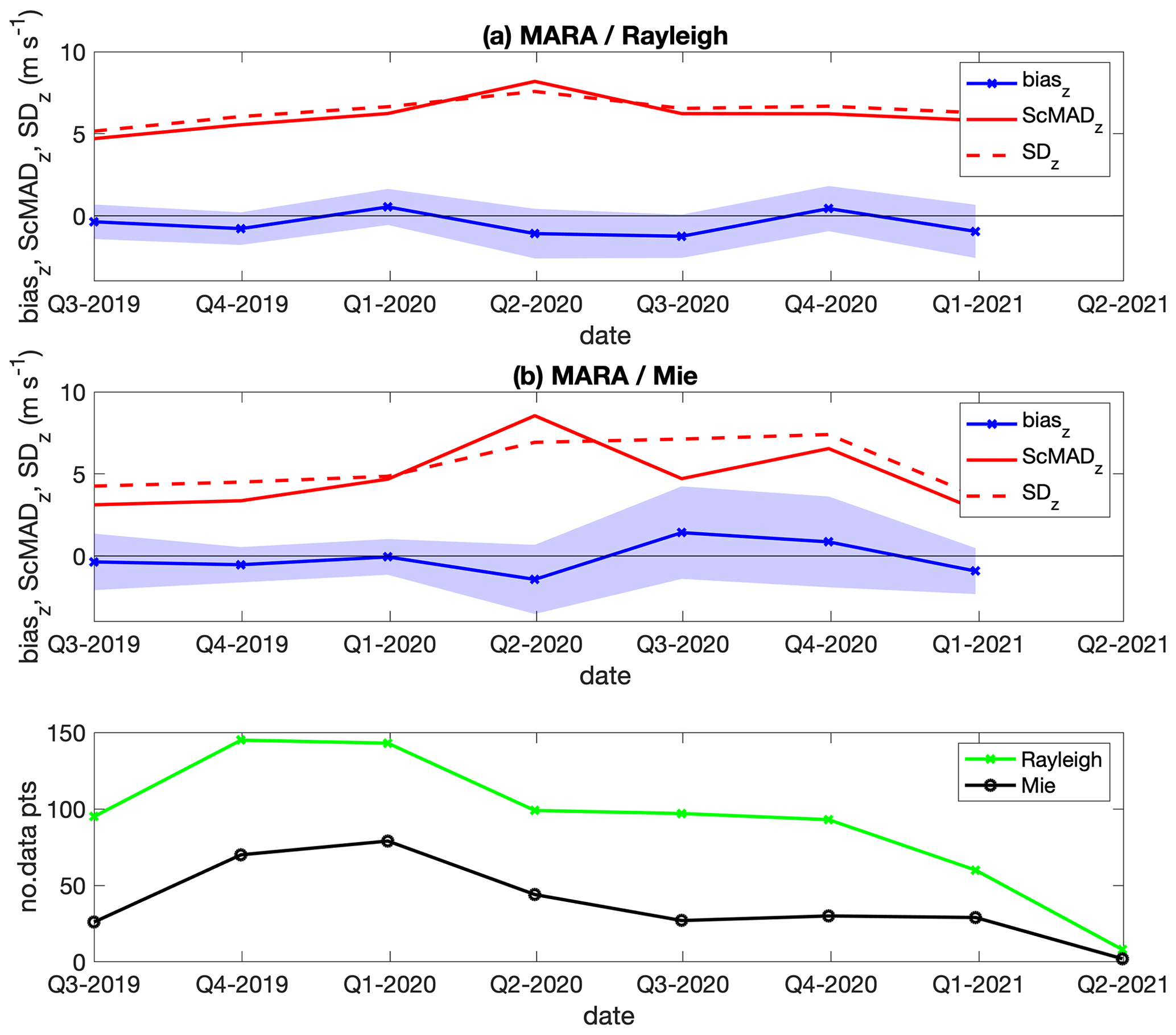
Figure 9 Variation over time of bias_z, ScMAD_z, and SD_z for the Aeolus–MARA comparison. The shaded area around bias_z indicates 95 % confidence limits. Each quarter (all seasons, all orbits) over the 2-year study period was processed separately. Insufficient data are available for the last quarter. The bottom plot shows the number of data points that are included in the comparison.

An alternative is to consider the effect on ScMAD_z of restricting the comparison to Aeolus wind measurements closer to the radars. These results are shown in the rightmost columns of Tables 1–4, where only Aeolus measurements with mid-points within 25 km of the radars are included. For Rayleigh winds, there is no improvement in ScMAD_z for the restricted dataset, but the long along-track averaging distance of the Aeolus Rayleigh winds means that they still include contributions from up to 68 km away. For the Mie winds, with a much shorter along-track averaging distance, there are improvements in ScMAD_z with the restricted dataset to 3.3 m s⁻¹ at MARA and 3.6 m s⁻¹ at ESRAD. This is well below the values for the other data subsets, which are 4.2–6.4 m s⁻¹ for MARA and 3.9–4.1 m s⁻¹ for ESRAD. It seems likely that spatial variability is an important contributor to ScMAD_z, particularly at MARA. The geometry of the orbit passes at MARA means that two passes per week within 100 km are ascending and two are descending. Only one (descending) pass per week comes within 25 km. The higher ScMAD_z for ascending compared to descending passes at MARA could be explained by 50 % of the descending passes being very close to the radar. Likewise, the much higher ScMAD_z for winter compared to summer at MARA may simply reflect higher spatial variability of the winds in winter, particularly as the comparison is primarily based on measurements from the lower troposphere. At ESRAD, three Aeolus orbits per week pass within 100 km, two descending (one to the east and one to the west) and one ascending (only the latter within 25 km). The only difference between the 25 km dataset and the full ascending dataset is the along-orbit distance included in the averaging for the comparison. The small improvement of ScMAD_z from 4.0 to 3.6 m s⁻¹ with the restricted dataset suggests that spatial variability along the orbit path contributes a little at ESRAD. There is no difference in ScMAD_z between ascending and descending passes, suggesting that along-orbit variability and east–west spatial variability are about the same. The slightly higher ScMAD_z for winter (4.1 m s⁻¹) compared to summer (3.9 m s⁻¹) may again be due to slightly higher spatial variability in winter.

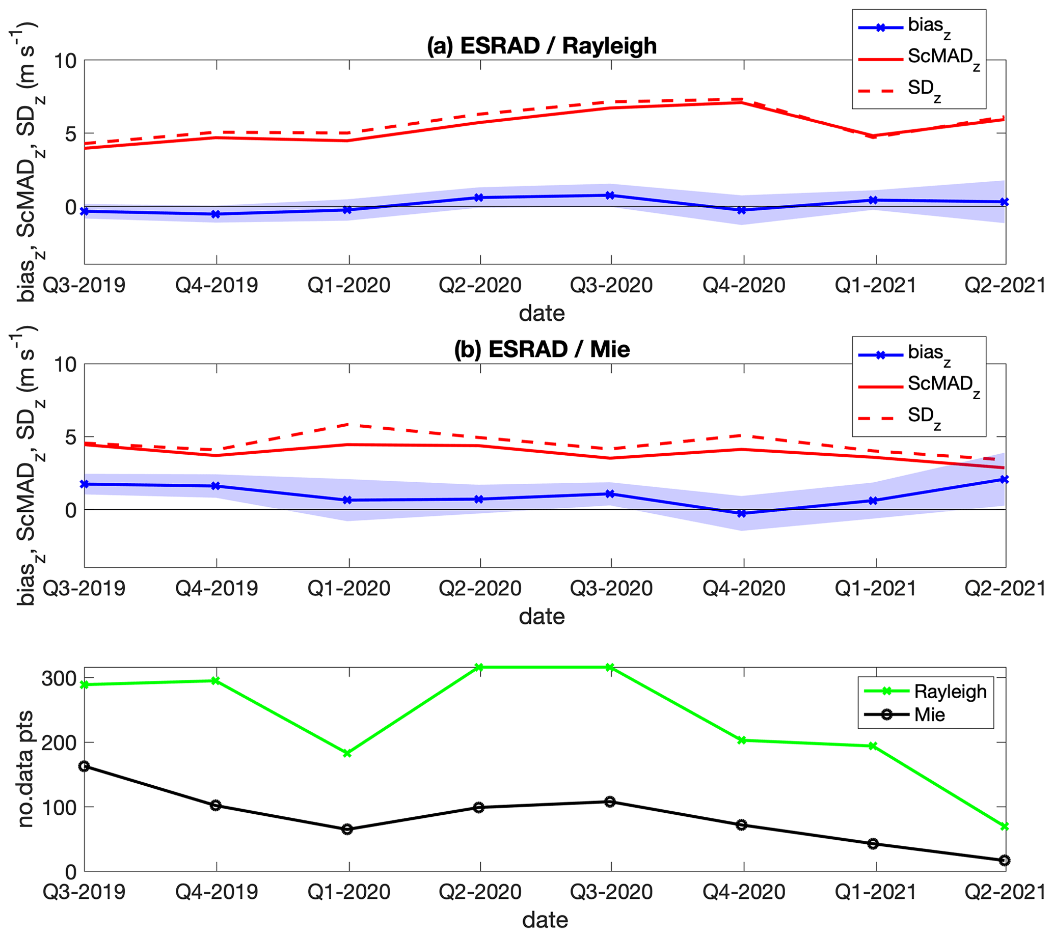
Figure 10 Variation over time of bias_z, ScMAD_z, and SD_z for the Aeolus–ESRAD comparison. The shaded area around bias_z indicates 95 % confidence limits. Each quarter (all seasons, all orbits) over the 2-year study period was processed separately. The bottom plot shows the number of data points that are included in the comparison.

The higher values for ScMAD_z for MARA compared to ESRAD (by 0.6–1.0 m s⁻¹) could be due to differences in local meteorology, leading to differences in spatial variability. The higher ScMAD_z for Rayleigh winds compared to Mie winds (by 1.0–1.4 m s⁻¹) is as expected because of different random errors in those wind estimates from Aeolus.

For the MARA and ESRAD data, Belova et al. (2021a) reported SD values for different subsets in the range 4–6 m s⁻¹ for Rayleigh winds and mostly 3–5 m s⁻¹ for Mie winds. The present study shows SD_z 5.5–6.8 m s⁻¹ for Rayleigh winds and 4.0–6.6 m s⁻¹ for Mie winds, which are somewhat higher. Figures 9 and 10 show how bias_z and its confidence limits as well as SD_z and ScMAD_z vary over the 2 years of the present study. These show an overall increase in confidence limits for bias_z for all cases, as well as in SD_z and ScMAD_z for Rayleigh winds. These are in line with the increase in estimated random errors for Aeolus winds between June 2019 and June 2021 (2B11 baseline) shown by Lux et al. (2022), which is due to degradation in power of the Aeolus lidar. There is no clear increase in SD_z and ScMAD for the Mie wind comparison, which could be due to the bigger influence of spatial variability on those values. We also note that the precision of Mie winds should be less affected by laser signal degradation as Mie winds are mainly retrieved form strong cloud scatter.