the Creative Commons Attribution 4.0 License.
the Creative Commons Attribution 4.0 License.
 | 21 Sep 2023
Long-term airborne measurements of pollutants over the United Kingdom to support air quality model development and evaluation
Angela Mynard
Joss Kent
Eleanor R. Smith
Andy Wilson
Kirsty Wivell
Noel Nelson
Matthew Hort
James Bowles
David Tiddeman
Justin M. Langridge
Benjamin Drummond
Steven J. Abel
The ability of regional air quality models to skilfully represent pollutant distributions throughout the atmospheric column is important to enabling their skilful prediction at the surface. This provides a requirement for model evaluation at elevated altitudes, though observation datasets available for this purpose are limited. This is particularly true of those offering sampling over extended time periods. To address this requirement and support evaluation of regional air quality models such as the UK Met Offices Air Quality in the Unified Model (AQUM), a long-term, quality-assured dataset of the three-dimensional distribution of key pollutants was collected over the southern United Kingdom from July 2019 to April 2022. Measurements were collected using the Met Office Atmospheric Survey Aircraft (MOASA), a Cessna 421 instrumented for this project to measure gaseous nitrogen dioxide, ozone, sulfur dioxide and fine-mode (PM2.5) aerosol. This paper introduces the MOASA measurement platform, flight strategies and instrumentation and is not intended to be an in-depth diagnostic analysis but rather a comprehensive technical reference for future users of these data. The MOASA air quality dataset includes 63 flight sorties (totalling over 150 h of sampling), the data from which are openly available for use. To illustrate potential uses of these upper-air observations for regional-scale model evaluation, example case studies are presented, which include analyses of the spatial scales of measured pollutant variability, a comparison of airborne to ground-based observations over Greater London and initial work to evaluate performance of the AQUM regional air quality model. These case studies show that, for observations of relative humidity, nitrogen dioxide and particle counts, natural pollutant variability is well observed by the aircraft, whereas SO2 variability is limited by instrument precision. Good agreement is seen between observations aloft and those on the ground, particularly for PM2.5. Analysis of odd oxygen suggests titration of ozone is a dominant chemical process throughout the column for the data analysed, although a slight enhancement of ozone aloft is seen. Finally, a preliminary evaluation of AQUM performance for two case studies suggests a large positive model bias for ozone aloft, coincident with a negative model bias for NO2 aloft. In one case, there is evidence that an underprediction in the modelled boundary layer height contributes to the observed biases at elevated altitudes.
- Article
(21175 KB) - Full-text XML
- BibTeX
- EndNote


The World Health Organization identifies atmospheric air pollution as the single largest environmental risk to human health globally (World Health Organization, 2017). Long-term exposure to anthropogenic air pollution is linked to increased morbidity rates and premature mortality from chronic diseases (Air Quality Expert Group, 2020; Manisalidis et al., 2020), which in the United Kingdom alone is estimated to have an annual impact on shortening lifespans, equivalent to 28 000–36 000 deaths (DEFRA, 2019). The impacts of air pollution on human health can be most acute in urban areas, particularly megacities, where high pollutant concentrations coincide with high population densities (Molina and Molina, 2004). In addition to impacting human health, air pollution has been shown to have wider detrimental impacts on ecosystems, including animal welfare, crop yields, waterways, biodiversity and visibility (DEFRA, 2019).
From an atmospheric sciences perspective, air pollution is a complex, transboundary problem. Gaseous and particulate pollutants originate from many sources, are subject to transport and mixing over a range of scales, and undergo complex physical and chemical processing prior to deposition. In order to develop effective strategies for mitigating the impacts of air pollution, for example through emission control and limiting population exposure, these processes must be understood and leveraged to provide predictive capability, extending spatially and temporally beyond the ground truth provided by observations. Atmospheric chemical transport models represent a key tool in this domain.
Air quality models vary widely in spatial scale and complexity and have evolved rapidly in sophistication in recent years. The reader is directed to El-Harbawi (2013) for a comprehensive review of air quality modelling systems that span scales from street canyons to global ones and incorporate a wide range of schemes representing pollutant emissions, turbulent mixing, advection, gas-phase chemistry and aerosol processes. Many of these models run online, meaning meteorological and pollutant fields evolve prognostically within the modelling system, allowing feedbacks between the two to be represented (such as direct and indirect aerosol effects) (Savage et al., 2013).
In the Met Office, the primary air quality modelling system is the Air Quality in the Unified Model (AQUM), a 12 km limited area forecast configuration of the Met Office Unified Model (MetUM). AQUM provides daily UK national air quality forecasts of the daily air quality index (DAQI) up to 5 d ahead (see https://uk-air.defra.gov.uk/forecasting/, last access: 11 September 2023), generated from the forecast of nitrogen dioxide (NO2), sulfur dioxide (SO2), ozone (O3) and particulate matter (diameters (Dp) < 2.5 µm: PM2.5 and Dp < 10 µm: PM10) concentrations. AQUM has eight vertical levels up to a model top height of 39 km, and mixing is parameterised throughout the full depth of the troposphere using a non-local, first-order closure, multi-regime scheme (Lock et al., 2000). Given the resolution of AQUM, it is best suited to modelling background and regional air quality away from strong, very localised sources of pollution (Neal et al., 2017; Williams et al., 2018). A comprehensive description of the AQUM is available in Savage et al. (2013).
Air quality models, including AQUM, require high-quality observations for development and evaluation. Given that air quality regulatory limits are imposed at ground level only, air quality model evaluation studies typically focus on assessment of performance using surface measurements. In the United Kingdom, these observations are commonly provided by the Automatic Urban and Rural Network (AURN), an automatic ground monitoring network operated on behalf of the UK Department of Environment, Food and Rural Affairs (Environment Agency, 2022).
Comparisons of AQUM to AURN observations (Savage et al., 2013; Neal et al., 2017) found that AQUM generally performed well, in particular for large air quality events, but had a number of systematic biases, including a positive bias in ozone at urban sites, a positive (negative) nitrogen oxide (NO2) bias at rural (urban) sites and small negative biases in PM2.5. These findings are generally comparable to similar air quality model evaluations that employ AURN observations, such as Williams et al. (2018) (10 km CMAQ-Urban model) and Neal et al. (2017) (HadGEM3-RA 50 km regional composition–climate model), although the latter showed a small positive bias in modelled PM2.5. For AQUM, ground-based observations are used to bias-correct the model data and minimise some of these systematic biases at the surface (Neal et al., 2014). Models that require bias correcting through assimilation with observations have the potential to introduce bias into future predictions, as assumptions that the same factors apply both now and in the future can be incorrectly made (Williams et al., 2018). We note that these biases may not solely be due to model performance and could also be partially attributable to difficulties in evaluating a 12 km resolution model with point observations that have limited spatial coverage, both in the horizontal (raising questions of representativity) and in the vertical (limiting model evaluation away from the surface–atmosphere boundary). These limitations in observational data currently available for model evaluation provide motivation for the current work, with a particular focus on the need for observations away from the surface. Given that vertical mixing serves to transport pollutants both away from and towards the surface and pollutant chemical, physical and removal processes occur throughout the atmospheric column, model skill in this domain is critical to achieving successful prediction at the surface (Solazzo et al., 2013).
Observations of pollutants throughout the atmospheric column are increasingly available from satellite instruments, e.g. TROPOMI on the European Space Agency's Sentinel-5P (Veefkind et al., 2012; Air Quality Expert Group, 2020; Wyche et al., 2021) and GOME on the European Space Agency's ERS-2 (Liu et al., 2005). While these observations can provide global coverage extending over timescales of years, they generally contain limited information on the vertical distribution of pollutants within the column (Fleming, 1996; Peers et al., 2019). Instrumented aircraft provide one way of addressing this gap. Over several decades, there have been a number of related large-scale initiatives to instrument in-service commercial aircraft to provide such measurements, e.g. Measurements of OZone, water vapour, carbon monoxide and nitrogen oxides by Airbus In-service airCraft (MOZAIC; Solazzo et al., 2013) and In-service Aircraft for a Global Observing System (IAGOS; Petzold et al., 2015). Over 44 000 flights have been conducted under IAGOS since 1994; though temporally and spatially restricted by commercial flight patterns and timings, these projects serve as a prime example of the use of instrumented aircraft to provide long-term observations for atmospheric model evaluation. An alternative approach is the use of atmospheric research aircraft, ARA, which are instrumented and deployed specifically for the pursuit of atmospheric science and monitoring. ARA deployments tend to focus on specific locations or events, and instrument payloads can vary greatly depending on the phenomenon under study. As such, while ARA are particularly well suited to the detailed study of chemical and physical processes (a key requirement for model development), the often-sporadic nature of their deployment limits the generation of consistent, long-term datasets. It is this gap that this work seeks to fill with a specific focus on air quality observations over the United Kingdom to allow for the evaluation of regional models such as AQUM.
The UK Clean Air: Analysis and Solutions research programme is led by the Met Office and the Natural Environment Research Council and has invested in modelling, data and analytical tools to assess current and future air quality and the impact of policies designed to improve it (DEFRA, 2019). Under this umbrella, a long-term, quality-assured dataset of the three-dimensional distribution of key pollutants (NO2, O3, SO2 and PM2.5) has been collected using the instrumented Met Office Atmospheric Survey Aircraft (MOASA). Observations have primarily covered the southern United Kingdom, including Greater London, with 63 flights throughout the period 2019–2022. This sampling period encompasses the global COVID-19 pandemic lockdown, when emission of primary pollutants significantly reduced as a result of limits on mobility throughout the United Kingdom. As such, the dataset may serve an additional application providing a unique resource with which to explore changes in atmospheric composition associated with reduced emissions during this period. This paper introduces the strategy and quality assurance basis for these observations and is not intended to be an in-depth diagnostic analysis, rather a comprehensive technical reference for all future users of these data, including illustrations of the potential uses of these upper-air observations for regional-scale model evaluation. In particular it includes descriptions of (i) the measurement platform and instrumentation, (ii) flight strategies, (iii) analysis of the spatial scales of measured pollutant variability, (iv) a comparison of ground-based observations to airborne observations from repeated flight patterns over Greater London and (v) initial use of these data to evaluate performance of the AQUM regional air quality model.
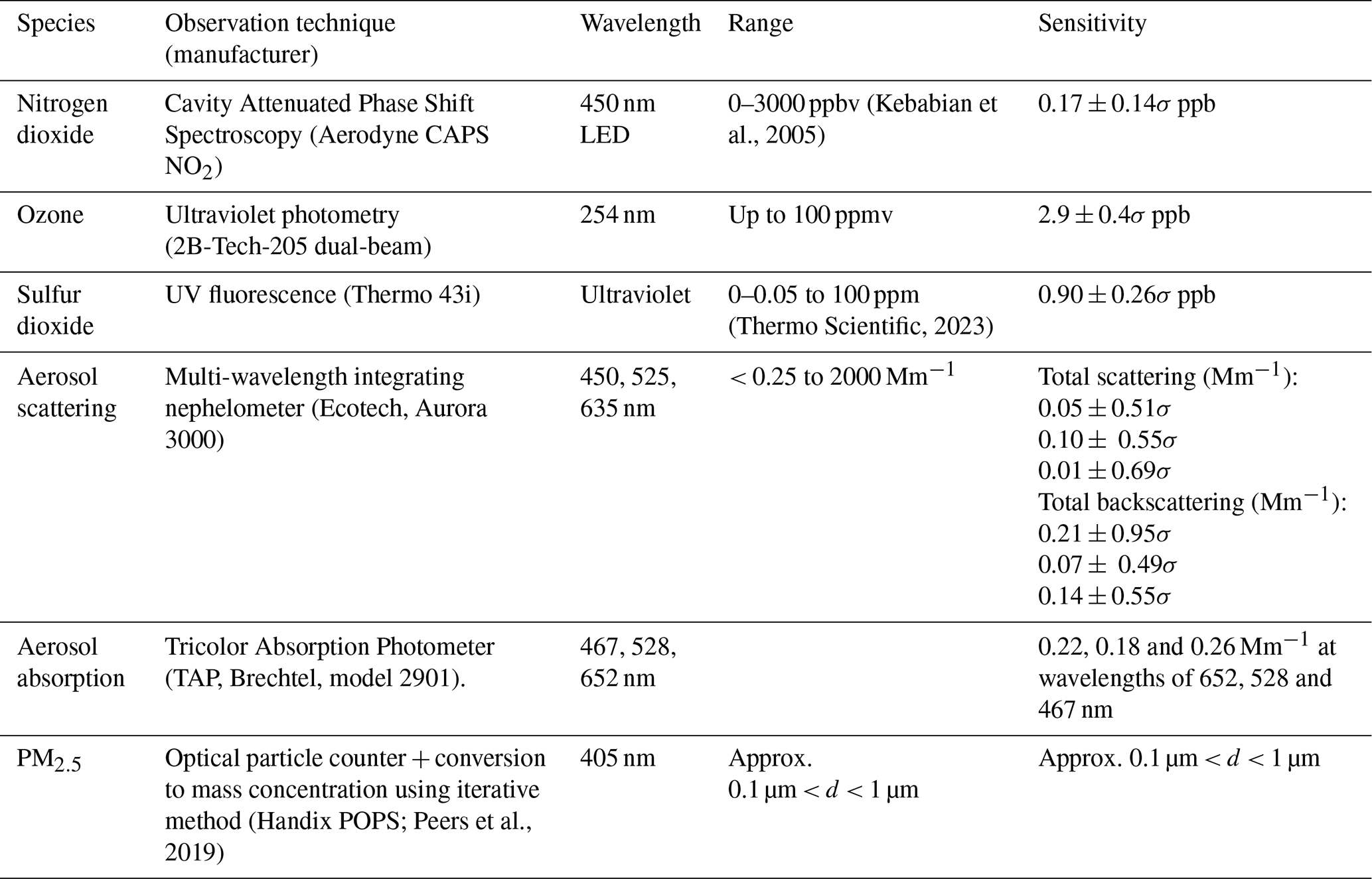
The MOASA, shown in Fig. 1, is a Cessna 421 aircraft based at Bournemouth Airport, operated by Alto Aerospace Ltd for the Met Office. The MOASA is instrumented to allow airborne measurement of key air-quality-relevant aerosol and gas phase pollutants: gaseous nitrogen dioxide (NO2), ozone (O3), sulfur dioxide (SO2) and fine-mode aerosol (PM2.5, determined indirectly from measurements of the aerosol size distribution). The fine-mode aerosol is also characterised in terms of optical absorption and scattering properties. This section provides a detailed description of the MOASA instruments (which are summarised in Table 1) and related quality assurance protocols.
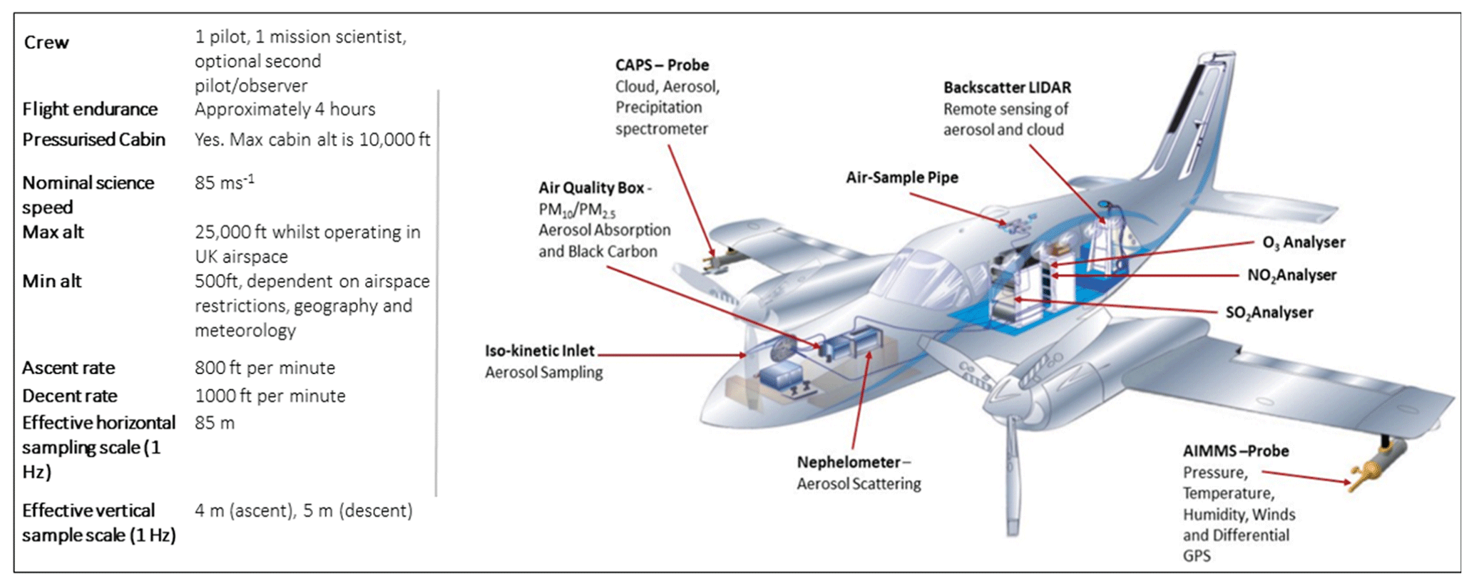
Figure 1The Met Office Atmospheric Survey Aircraft, with instrumentation. The aircraft has a maximum cabin altitude of 3048 m, a maximum (minimum) altitude of 7620 m (152 m) and an ascent (descent) rate of 243 m (300 m). Image courtesy of Debbie O’Sullivan, Met Office, 2021.
2.1 Instrument overview
Instruments, examples of which can be seen in Fig. 2, are situated in the cabin, the front hold of the aircraft and under the wings. Wing-mounted probes include the Aircraft-Integrated Meteorological Measurement System (AIMMS, Aventech) instrument that provides real-time ambient meteorological data including temperature, humidity, pressure and three-dimensional winds (speed, direction, vertical) as well as latitude, longitude and (GPS) altitude. The aircraft also includes a wing-mounted Cloud, Aerosol and Precipitation Spectrometer with Particle-By-Particle (Droplet Measurement Technology) though it does not form part of the air quality measurement suite and therefore is not discussed further here. Nitrogen dioxide, ozone and sulfur dioxide instruments are rack mounted in the cabin and sample at 0.85, 1.8 and 0.5 L min−1, respectively. All instruments have a 1 Hz sampling resolution, except for the O3 monitor, which samples at 0.5 Hz. Ambient gaseous samples are drawn from a stainless-steel air sample pipe that takes air from outside of the fuselage boundary layer through an on-rack PTFE headed sample pump (KNF N834.3FTE). Also within the cabin is a backscatter aerosol lidar (Leosphere), which is used operationally though it does not form part of the core air quality measurement suite. The starboard side nose bay compartment contains a custom-built “air quality box” (AQ box) and a nephelometer (Ecotech, Aurora 3000) (Fig. 2). The air sample to each of the instruments in the front hold is controlled by actuated valves and volume flow controllers inside the AQ box (see Appendix A).
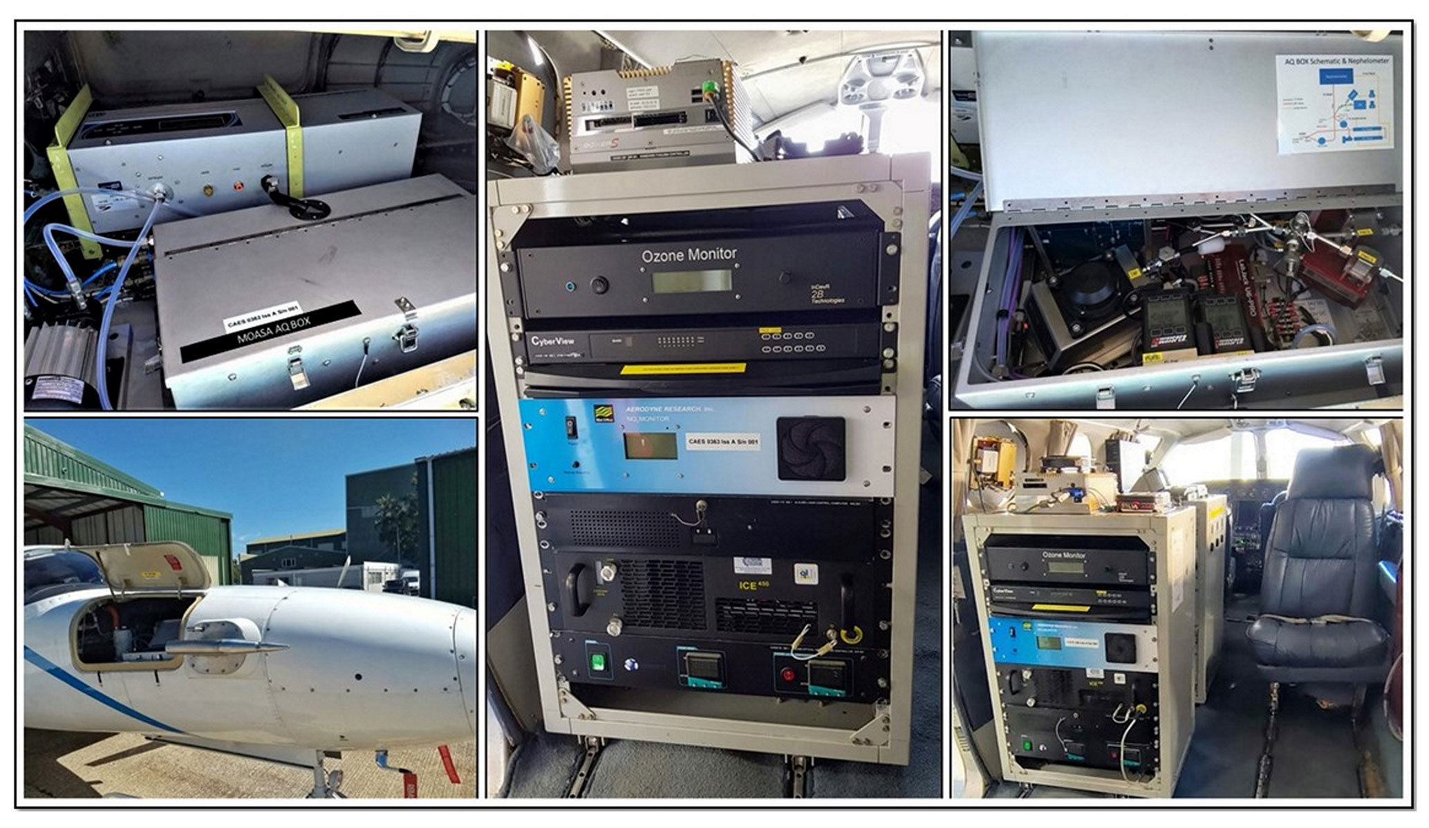
Figure 2Upper left: the AQ box (foreground) and nephelometer (background) in the MOASA nose bay. Lower left: the Brechtel isokinetic air sample inlet alongside the nose bay of the MOASA. Middle: the aft instrumented rack, housing the O3, NO2 and aerosol lidar control system. Upper right: inside the AQ box and lower right inside the cabin looking forward.
The AQ box contains a Portable Optical Particle Spectrometer (POPS, Handix) and a Tricolour Absorption Photometer (TAP, Brechtel, model 2901) and has the capability to subselect only PM2.5 sample aerosols for analysis. The sample in the AQ box is from a Brechtel isokinetic inlet, which samples at 6.35 L min−1 and has a > 95 % sampling efficiency for particle diameters from 0.1 to 6 µm (Brechtel Manufacturing Inc, 2011). The PM2.5 sample flow is dried via two Perma Pure MD-700 driers, connected in series via a 180∘ bend. The sample then passes through an impactor with an aerodynamic cut point size of 2.5 µm, before being split between the POPS (0.5 L min−1 (sample + sheath)), TAP (1 L min−1) and the nephelometer (5 L min−1), which is situated alongside the AQ box. Measurements at the nephelometer and TAP inlet indicate that the PM2.5 sample relative humidity is typically below 20 %, and therefore the sample is a good representation of the dry-PM2.5 size distribution. Within the AQ box the sample line temperature and pressure are also recorded.
Particle losses through the PM2.5 sampling lines have been estimated using open-access particle loss calculation software (von der Weiden et al., 2009) based on the tubing dimensions, flow characteristics and a representative particle density of 1.64 g cm−3. This analysis has suggested losses downstream of the inlet of < 17 % for particle diameters in the range 0.1–3 µm.
In addition to particle losses due to flow deposition, we have considered the extent to which loss of particle mass may occur due to evaporation of ammonium nitrate, NH4NO3, a semi-volatile aerosol component that readily repartitions between condensed and gas phases upon changes in temperature and humidity (Nowak et al., 2010; Langridge et al., 2012; Morgan et al., 2010). To determine the fractional loss of NH4NO3 during MOASA sampling, a kinetic model of the NH4NO3 evaporation process (based on the approach of Fuchs and Stutugin, 1971, as implemented by Dassios and Pandis, 1999) was used to calculate the rate of change in diameter of polydisperse NH4NO3 particles through the MOASA flow system. The model unsurprisingly showed that the loss of particulate nitrate had a strong temperature dependence and varied dynamically as a function of time. Total mass losses during the MOASA sampling residence time of 2 s and at a representative sampling temperature of 30 ∘C were approximately 7 %. The NH4NO3 losses showed a weak dependence on pressure and relative humidity, with absolute losses increasing by only 2 % at 500 Mbar compared to 100 Mbar and by approximately 2 % over the relative humidity (RH) range 10 %–50 % (where in-flight PM2.5 sample RH was typically below 20 %). Although evaporative loss of NH4NO3 during MOASA sampling will vary on a case-by-case basis, for representative conditions this work confirms that the loss is small and likely less than 7 %.
The AQ box also allows for measurement of the aerosol population without particle size selection or drying. However, this mode of operation has not been utilised in this work and is therefore not described further.
2.2 Nitrogen dioxide
A cavity attenuated phase shift spectroscopy nitrogen dioxide detector (Aerodyne Research Inc, referred to here as NO2CAPS) was repackaged in-house, from a 5 U, 12 kg to a 3 U, 9.7 kg 19 in. (48 cm) rack-mounted unit to optimise volume and weight for airborne use. The analyser monitors ambient atmospheric NO2 concentrations, with a lower detection limit of < 1 parts per billion (ppb), using a 450 nm LED-based absorption spectrometer utilising cavity attenuated phase shift spectroscopy (Kebabian et al., 2005). A comprehensive review of the theory of operation is detailed in Kebabian et al. (2005). The NO2CAPS analyser has been shown to be insensitive to other nitro-containing species and variability in ambient aerosol, humidity and other trace atmospheric species (Kebabian et al., 2005).
While some cavity-based absorption techniques are often referred to as calibration free (Langridge et al., 2008), this feature relies on knowledge of the variation in absorption cross section across the spectral range of the light source being used. Given the broadband nature of the NO2CAPS light source, which is difficult to characterise accurately and may be subject to change over time, we chose to undertake routine direct calibration of the instrument. As such, full multi-point calibrations are carried out annually at the National Centre for Atmospheric Science (NCAS) Atmospheric Measurement and Observation Facility (AMOF) COZI Laboratory at the University of York. Here, a multi-gas calibrator is used to dilute a high-concentration NO standard into zero air (grade Pure Air Generator 001) at varying levels. Ozone is added in excess to ensure full conversion of NO to NO2. Seven concentration levels are used, and zero checks are also carried out. Calibration coefficients are determined from linear fits and applied to the NO2CAPS during data post-processing.
NO2 analyser baseline pressure dependency correction
During normal operation, the NO2CAPS analyser periodically establishes a baseline to account for the optical losses associated with light transmission by the cavity mirrors (which depend both on mirror cleanliness and alignment) and Rayleigh scattering of light by air (Kebabian et al., 2005). This is achieved by passing NO2 free air through the analyser every 15 min (automated). The standard NO2CAPS software then applies a constant baseline correction based on these periodic measurements for the sampling segment that follows. For variable-pressure aircraft operation, this approach is not adequate as changes in Rayleigh scattering that accompany pressure changes lead to shifts in the instrument baseline between filter periods.
To account for these changes, a new correction scheme has been developed. During post-processing, the pressure dependence of the baseline is determined by applying a linear fit to the pressure variation in Rayleigh-corrected filtered-air measurements recorded across the full flight. This dependence is used to calculate a new time-varying baseline based on sample pressure measurements alone. This baseline is then used to recalculate the NO2 concentration across the flight. Spikes due to valve switches are also removed from the data series at this stage.
Figure 3 shows raw (red) and processed (blue) NO2 concentration during flight M304 in November 2021, where the NO2CAPS sample inlet was fitted with a zero-air filter such that measurements were sensitive only to baseline changes. Following take-off at 11:52:00 UTC the aircraft climbed to an altitude of 5.5 km, resulting in an ambient pressure change of 509 Mbar and a NO2CAPS measurement–cell-pressure change of 250 Mbar. The profile shows that corrected data are markedly more stable in comparison to the raw data and suggests a mean error in NO2 concentration due to pressure-dependent baseline corrections of ±0.09 ppbv (data averaged over 10 s intervals). The sensitivity of the NO2CAPS was empirically derived to be 0.17 ± 0.14σ ppbv (during a separate ground-based zero test, where data are also averaged over 10 s intervals). As such, following correction, NO2CAPS pressure sensitivity is not considered a significant source of uncertainty for aircraft NO2CAPS observations.
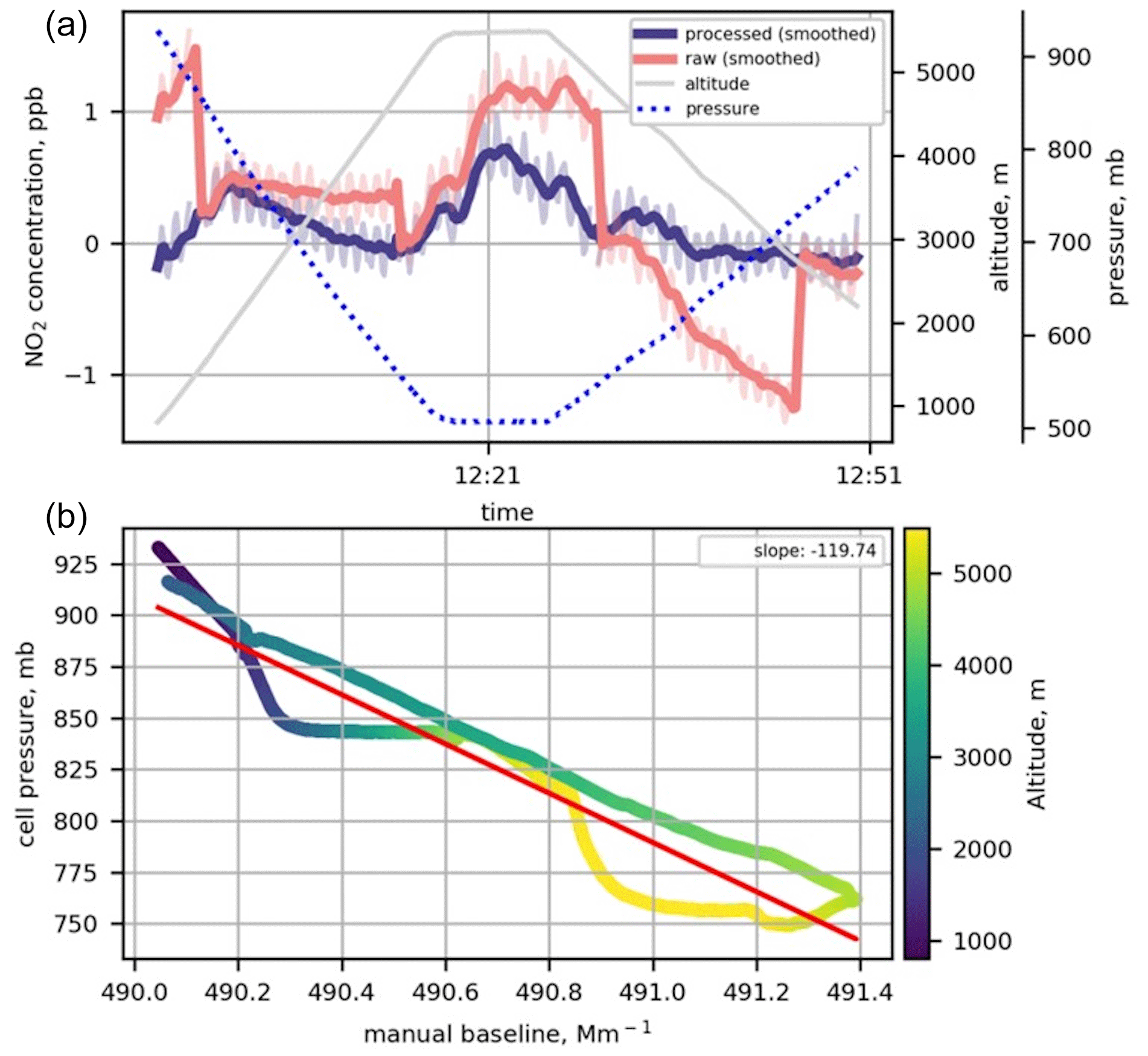
Figure 3(a) Time series of raw (uncorrected) and processed (corrected) NO2 concentration. Oscillations seen in the raw and processed data during the filter test are an artefact of the filter, which impacted performance of the instrument pump. These oscillations have been minimised by arbitrarily smoothing (60 s rolling). The data are for visualisation purposes only. (b) Baseline against cell pressure, coloured by altitude, with a linear fit is shown as a red line. All data from 11:55:00 to 12:50:00 UTC during flight M304 on 4 November 2021 are averaged over 10 s intervals.
2.3 Ozone
A dual-beam ozone monitor (2B Tech, model 205) enables measurements of atmospheric ozone up to 100 ppmv (parts per million by volume). Measurements are based on the absorption of ultraviolet (UV) light at 254 nm in two absorption cells: one with ozone-scrubbed (zero) air and one with unscrubbed (sample) air from which the Beer–Lambert law can be used to determine ozone concentration. The instrument sensitivity, empirically derived by sampling filtered air at 0.5 Hz during a test flight, is 2.9 ± 0.4σ ppb. The monitor is calibrated annually at the NCAS AMOF COZI Laboratory, where the instrument is compared with a NIST-traceable standard ozone spectrometer over a wide range of ozone mixing ratios. These results are used to calibrate the ozone monitor with respect to gain and sensitivity, which are applied to the instrument directly.
A known but not widely recognised issue with UV absorption ozone monitors is that rapid changes in humidity (as may occur during airborne ascents and descents) can cause a large zero shift. This is due to modulation of humidity of the sample stream by the ozone scrubber, which can cause the humidity in the sampling and zero cells to go out of equilibrium. To equilibrate the humidity, Nafion tubes known as DewLines are used in the 2B Tech monitor (Dewline, 2020; Wilson and Birks, 2006). Biases may become apparent should the DewLines stop working effectively; thus, following some initial issues with negative calculated ozone values during MOASA measurements (impacting the first seven flights, which do not have valid ozone data), the DewLines were regularly replaced.
2.4 Sulfur dioxide
A pulsed florescence SO2 analyser (Thermo Scientific, 43i Trace Level-Enhanced) detects sulfur dioxide up to 1000 ppbv. It operates on the principle that SO2 molecules fluoresce following absorption of ultraviolet light, with the fluorescence intensity proportional to the number of SO2 molecules in the air sample (Beecken et al., 2014). The instrument sensitivity was empirically determined using zero-air checks to be 0.90 ± 0.26σ ppb (averaged over 10 s intervals). The SO2 instrument is calibrated (zero and span) monthly in the field using an 863 ppb BOC alpha standard gas.
2.5 Aerosol scattering
A multi-wavelength integrating nephelometer (Ecotech, Aurora 3000) measures the light-scattering coefficient of the aerosol population in both forward- and back-scatter directions. It uses three high-power LED sources operating at wavelengths of 450, 525 and 635 nm.
Instrument sensitivity, determined from baseline statistics when sampling filtered air over 30 min at wavelengths of 450, 525 and 635 nm, was 0.05 ± 0.51σ, 0.10 ± 0.55σ and 0.01 ± 0.69σ Mm−1 for total scattering and 0.21 ± 0.95σ, 0.07 ± 0.49σ and 0.14 ± 0.55σ Mm−1 for backscattering, respectively (data averaged over 10 s intervals). This falls within the manufacturer-specified sensitivity of < 0.3 Mm−1. A monthly CO2 calibration and annual in-house service are completed for the nephelometer as per manufacturer procedures (Ecotech, 2009).
Uncertainties in scattering measurements using the nephelometer are dependent on sample flow (empirically derived over all flights as < 0.05 %), the uncertainty of calibration, inhomogeneities in Lambertian angular illumination and truncation of light due to cell geometry. Corrections for angular truncation and non-Lambertian light source effects are applied according to the recommendations of Müller et al. (2011).
Müller et al. (2011) empirically calculated an uncertainty of 4 % (450 nm), 2 % (525 nm) and 5 % (635 nm) for total scattering and 7 % (450 nm), 3 % (525 nm) and 11 % (635 nm) for total backscatter, which are adopted here. The signal-to-noise ratio for backscattering is worse than for total scattering, since the backscattering signal is about 1 order of magnitude smaller than the total scattering signal for ambient air (Müller et al., 2011).
2.6 Aerosol absorption
Aerosol absorption is measured using a Tricolor Absorption Photometer (TAP, Brechtel, model 2901). The TAP is a three-wavelength (467, 528, 652 nm) filter-based absorption photometer which derives real-time aerosol light absorption from the difference in light transmission measured between two 47 mm diameter Pallflex (E70-2075W) glass-fibre filter spots, one of which receives particle-laden air and the second of which receives aerosol-filtered air (Davies et al., 2019; Bond et al., 1999; Perim De Faria et al., 2021; Ogren et al., 2017). The TAP employs empirical corrections to account for scattering effects that complicate the derivation of aerosol absorption from filter transmission measurements. The theory of operation and characterisation of the TAP is given in Ogren et al. (2017) and Davies et al. (2019) (where it is previously known as a “CLAP”).
Mean 1σ detection limits of the MOASA TAP, empirically derived by sampling filtered air and averaging over 60 s, are 0.22, 0.18 and 0.26 Mm−1 at wavelengths of 652, 528 and 467 nm, respectively. These values are in line with the manufacturer-provided noise level characterisation of 0.20 Mm−1 over the same integration time.
The errors in absorption measurements from filter-based photometry are dominated by uncertainties in the empirical scattering corrections and also have contributions from uncertainties in the spectral response of the light source (±1–2 nm; Ogren et al., 2017), sample flow rate (< 1 %; Ogren et al., 2017), filter spot size and the penetration depth of particles within the filter matrix (Bond et al., 1999; Davies et al., 2019; Müller et al., 2014; Virkkula, 2010; Ogren et al., 2017). Internal particle losses within the instrument flow system due to diffusion, impaction and sedimentation are estimated to be < 1 % for particles with diameters in the range 0.03–2.5 µm (Davies et al., 2019; Ogren et al., 2017). To minimise the effects of instrument noise observed in-flight, a low-pass filter is applied to raw data with a cut-off frequency of 0.08 Hz, although this had minimal impact on optical properties derived from these data.
We apply scattering corrections to the low-pass-corrected TAP data using the Virkkula (2010) correction scheme, which relies on simultaneous measurements of the light-scattering coefficient, which in this case are provided by the nephelometer. The correction scheme is implemented as described by Davies et al. (2019). Ogren et al. (2017) provided an estimate of the accuracy of TAP absorption measurements of 30 %, and this value is adopted here. However, as summarised by Davies et al. (2019), given the empirical nature of filter-based correction schemes and strong source and wavelength dependencies, these correction schemes are unlikely to fully bound uncertainties associated with filter-based absorption measurements.
2.7 Aerosol size distributions
A portable optical particle counter (POPS, Handix) measures the size of dried particles predominantly in the accumulation mode (approximately 0.1 µm < d < 1 µm) (Haywood, 2008) using a light-scattering technique. The POPS uses a spherical mirror to collect a fraction of light scattered sideways (38–142∘) by individual particles traversing a 405 nm laser beam. The scattered light is directed to a photomultiplier tube, the signal from which is digitised and placed into 1 of 32 bins that are spaced logarithmically in scattering amplitude space. For a given laser power, the measured scattering amplitude is determined by the particle size, shape and index of refraction (IOR), thus allowing the bin boundaries to be converted to effective particle size subject to assumptions about shape and optical properties. In addition to particle size, given the POPS is a single particle instrument, it also provides a measure of the total particle number within its detection size range. A comprehensive review of POPS theory of operation is provided by Gao et al. (2016).
2.7.1 Calibration
Particle sizing by the POPS is calibrated by measuring the scattering amplitude of atomised NIST-traceable polystyrene latex (PSL) spheres of known size, spherical shape and IOR (Rosenberg et al., 2012; Peers et al., 2019; Gao et al., 2016). Calibrations use 10 discrete sizes of PSL between 0.15 and 3 µm. The PSL is atomised and dried prior to entering the POPS sample inlet. PSL sizes between 0.15 and 0.70 µm are, where possible, also passed through a differential mobility analyser (TSI 3082 Electrostatic Classifier) in order to help minimise the impacts of contaminants from the PSL generation process.
For each PSL diameter, Mie theory is used to calculate the particle-scattering cross section (Fig. 4), using a PSL IOR at 405 nm of 1.615 + 0.001j (Gao et al., 2016). Linear regression is then used to fit the relationship between the POPS-measured scattering amplitude and the theoretical PSL scattering amplitude (Rosenberg et al., 2012). The error in response is determined from the standard error in the mean for each 15 s period of sampling, averaged over the duration of the PSL run. The error in PSL diameter is the NIST-certified range of the PSL diameter. The linear regression function is used to assign calibrated scattering amplitudes to the designated POPS bin boundaries. At this point, the POPS measurements are calibrated.
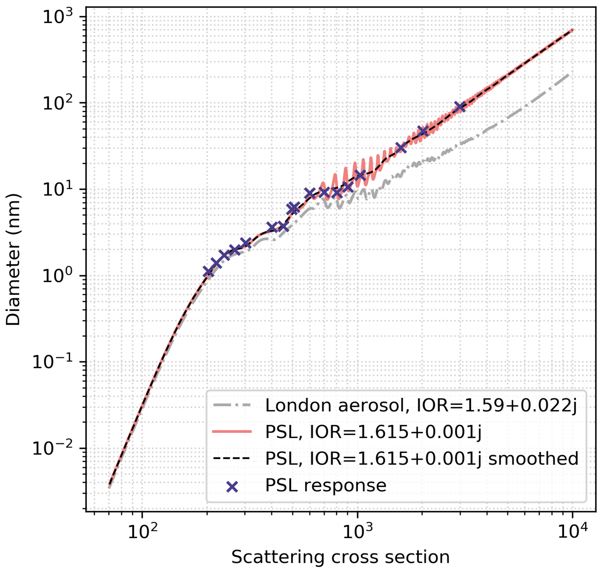
Figure 4Theoretical MOASA POPS Mie responses for PSL calibrant (1.615 + 0.001j) and ambient aerosol over London: 1.59 − 0.022j (McMeeking et al., 2012). Crosses are PSL responses from calibration on 16 September 2021.
To size ambient particles, it is necessary to convert the bin boundaries to equivalent diameters for particles with different optical properties. The impact of particle index of refraction on the POPS response is shown in Fig. 4, which shows the relationship between particle diameter and theoretical POPS response for both PSLs and particles representative of urban sampling. To account for the significant differences seen, we again apply Mie theory. The calibrated POPS bin boundaries in scattering cross-section space are converted to diameter space based on Mie calculations. These calculations integrate scattering over the angular range of collection angles of the POPS and use an estimate of the ambient particle IOR (further details below) (Rosenberg et al., 2012; Gao et al., 2016). To overcome inherent Mie resonance oscillations in calculated scattering signals (where Dp > 600 nm in Fig. 4), which result in non-monotonic behaviour with increasing particle diameter (Gao et al., 2016; Rosenberg et al., 2012), each Mie response curve is smoothed using spline interpolation (Hagan and Kroll, 2020). As particle morphology and inter- and intra-particle homogeneity of the ambient sample are unknown, an assumption of spherical, homogeneous particles is implicit to the application of this Mie-theory-based approach.
2.7.2 Index of refraction
The IOR of the aerosol sample used for determination of POPS bin boundaries for ambient sampling is estimated using the method described in Liu and Daum (2000) and Peers et al. (2019). This is an iterative approach whereby the single-scattering albedo (the wavelength-dependent ratio of aerosol scattering to total extinction, ω0) is calculated from the dry-POPS particle size distribution (ω0psd, λ = 405 nm) using an initial-guess IOR and then compared to the measured single-scattering albedo at 405 nm derived from independent observations from the MOASA nephelometer and TAP (ω0nt). The IOR is then adjusted iteratively until acceptable closure is reached between calculated and measured ω0, noting that the POPS bin boundaries are adjusted upon each iteration. This process is summarised in Fig. 5; more details, including a case study, are in Appendix B.
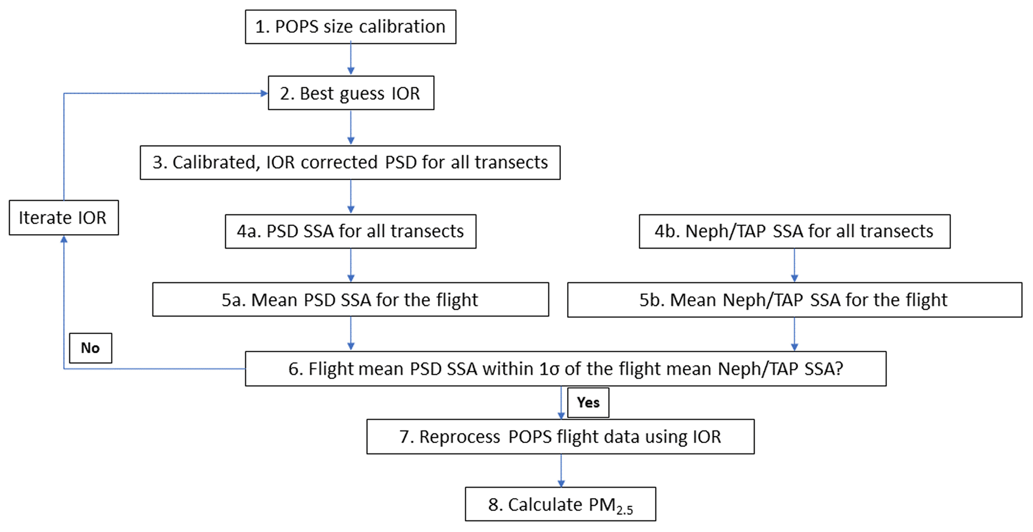
Figure 5Process to estimate the IOR of the ambient sample by iteratively adjusting the index of refraction of the POPS size distribution measurements until the POPS single-scattering albedo matches the single-scattering albedo from the nephelometer and TAP.
A strength of the MOASA dataset is that the POPS, TAP and nephelometer all share a common sample inlet, which reduces the potential source of sampling bias that may impact this analysis. Further, to minimise differences in sampling volumes and response times, all ω0 calculations are performed using 30 s averaged data, and only data from straight and level runs (SLRs; flight transects at approximate constant altitude and velocity) of at least 3 min duration are included. The iterative IOR analysis step is performed on the flight mean of these SLR data. While this approach does not allow in-flight variability to be accounted for, it minimises potential for erroneous impacts on the POPS size distribution arising from noise and uncertainty in the ω0 measurements, which can be large at low aerosol loading levels. The flight-average approach adopted here has been shown to lead to modest errors in particle diameter of < 10 % compared to analysis at finer temporal scales (see case study in Appendix B). We also note that while the IOR derived here provides closure between MOASA optical instruments, it is subject to potential uncertainties, such as assumptions of aerosol homogeneity and sphericity, and we caution against its use as an accurate measure of the true ambient particle IOR (Frie and Bahreini, 2021).
2.7.3 Size distribution uncertainties
A review of uncertainties for the POPS instrument is given in Gao et al. (2016). For particle number measurements, the main source of uncertainty for particles within the instrument's size detection range is the sample flow rate. Gao et al. (2016) report a nominal sample flow rate of 3 cm3 s−1 with an upper limit of 6.67 cm3 s−1 and an associated error of < 10 % (Gavin McMeeking at Handix, personal communication, October 2020). For the MOASA POPS the sample flow over all flights ranged from 2.7 to 5.9 cm3 s−1 (data averaged over 10 s intervals). The higher values arose due to flow system cross-interference issues that generated flow noise impacting the first 11 MOASA flights, following which the source of noise was removed and a more representative range of normal operation was 2.9 cm3 s−1 ± 3.2 %.
Coincidence errors, whereby two or more particles traverse the laser beam at the same time leading to sizing errors, are a common feature of all optical particle counters when used in high-aerosol-loading environments. The impact of coincidence errors on the MOASA POPS observations is addressed during data processing by flagging all data in which particle concentrations exceed 7000 cm3 s (Gavin McMeeking at Handix, personal communication, 2020).
Particle sizing uncertainties arise from a number of sources, including scattering amplitude measurement uncertainty (leading to an estimated 3 % 1σ sizing error for 500 nm particles) and laser intensity instability (±3 % diameter sizing error for temperatures from 43 to 46 ∘C). In addition, for reasons already discussed above, uncertainty in the IOR of particles being measured also impacts uncertainty in particle sizing. Gao et al. (2016) used a theoretical ambient aerosol population to investigate the potential magnitude of this error. They assessed the accuracy in the location and width of lognormal fits to both a theoretical population fine mode (10 % and 10 % respectively) and coarse mode (1.4 % and 19 % respectively). These uncertainties were propagated to derive an estimated uncertainty in the total particle volume of 19 %. Though based on a single theoretical ambient size distribution, this analysis provides an indication of the magnitude of error arising from IOR variation. For MOASA POPS-derived size distributions, it is likely to provide an upper indication of the error, given that efforts to correct the POPS bin boundaries based on the iterative IOR method described above should serve to improve sizing accuracy.
Based on the information above, an upper estimate for the error in total particle volume from POPS measurements (required for subsequent calculation of particle mass) is derived by combining in quadrature contributions from IOR (19 %), sample flow (3.2 %) and laser amplitude (6 %) to yield an uncertainty of 20 %.
2.8 Determination of mass concentration (PM2.5)
To calculate particulate mass, we convert the calibrated, IOR-corrected POPS particle size distributions to volume distributions and subsequently mass distributions by assuming a fixed particle density. The total mass is then calculated by integrating across the distribution within the PM2.5 size range. Calculations are performed on 10 s averaged data and work on the basis of fitting lognormal functions to the measured distributions to represent a fine and coarse mode (the dashed line in Fig. 6 shows the combined lognormal modes from a straight and level run during flight M270 on 15 September 2020). This approach serves to reduce the impact of residual structure from Mie resonances in the POPS distribution on mass derivations.
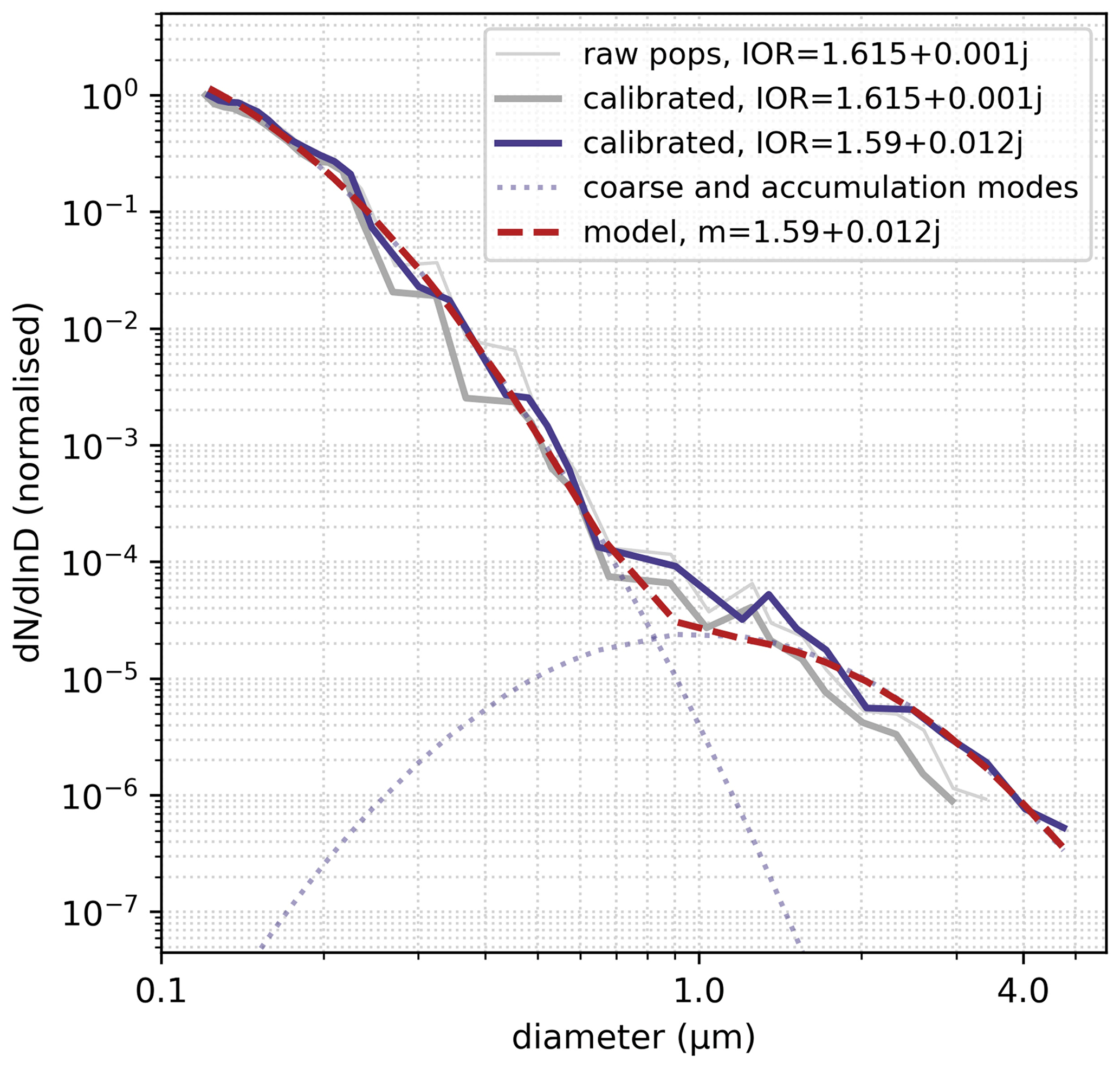
Figure 6An example of raw, calibrated (no IOR correction) and calibrated with IOR correction (IOR = 1.59 + 0.12j) particle size distributions, where the y axis is normalised to 1. Overlaid are lognormal accumulation and coarse modes (dotted) plus the combination of these lognormal modes (dashed) fitted to the calibrated with IOR correction (blue solid line) size distribution.
The selection of an appropriate particle density for converting volume to mass is an important part of the above analysis. The composition and therefore density of ambient aerosol vary dynamically in the atmosphere (Hinds, 1999; Crilley et al., 2020). In the absence of co-located aerosol composition observations on MOASA, we apply a fixed density to all data of 1.64 ± 0.07 (1σ) g cm−3. This value is derived by weight averaging the densities of PM2.5 aerosol components measured during a range of UK field experiments, as detailed in Appendix C.
The total uncertainty in the determined PM2.5 mass concentration, estimated by combining uncertainties in the measured particle volume (20 %) and the assumed particle density (4.2 %), is 20.4 % and thus dominated by the volume error.
The MOASA air quality flight strategy was based on flying a series of repeated sorties, each designed to provide data suitable for various aspects of model evaluation work. On a week-to-week basis, sorties were selected based on the prevailing weather conditions, and any required modifications to flight plans were made at that time. This section describes the rationale behind each of the sortie types, together with a summary of flight activities.
Given the MOASA home base is at Bournemouth on the south coast of the United Kingdom, operations have predominantly focused on sampling over the south of the United Kingdom. This includes work over the English Channel (e.g. sampling transboundary pollution), over varied land-use types (urban and rural) including pollution hotspots such as London, and over isolated source regions such as docks and industrial sites. In addition to regular sorties, in June–July 2021 (summer) and January–March 2022 (winter), the MOASA also participated in intensive observation periods (IOPs) in conjunction with ground-based Integrated Research Observation System for Clean Air (OSCA) air quality supersites, located in London, Birmingham and Manchester (UKRI, 2021; OSCA, 2020). All flights are performed within operational airspace regulations which limit minimum and maximum flight levels. Observations are mostly in the boundary layer and, as shown in Fig. 7, bottom panel, typically near or below 1 km GPS altitude. The lowest altitudes (0.15 km minimum) are permitted in offshore and rural areas, whereas minimum altitudes in urban areas (or in regions with significant topography or obstacles like masts or chimneys) are limited to > 0.3 km. Where possible profile measurements extending into the free troposphere are also collected, which allow the boundary layer height to be determined in addition to sampling of aged and/or transported pollutants.
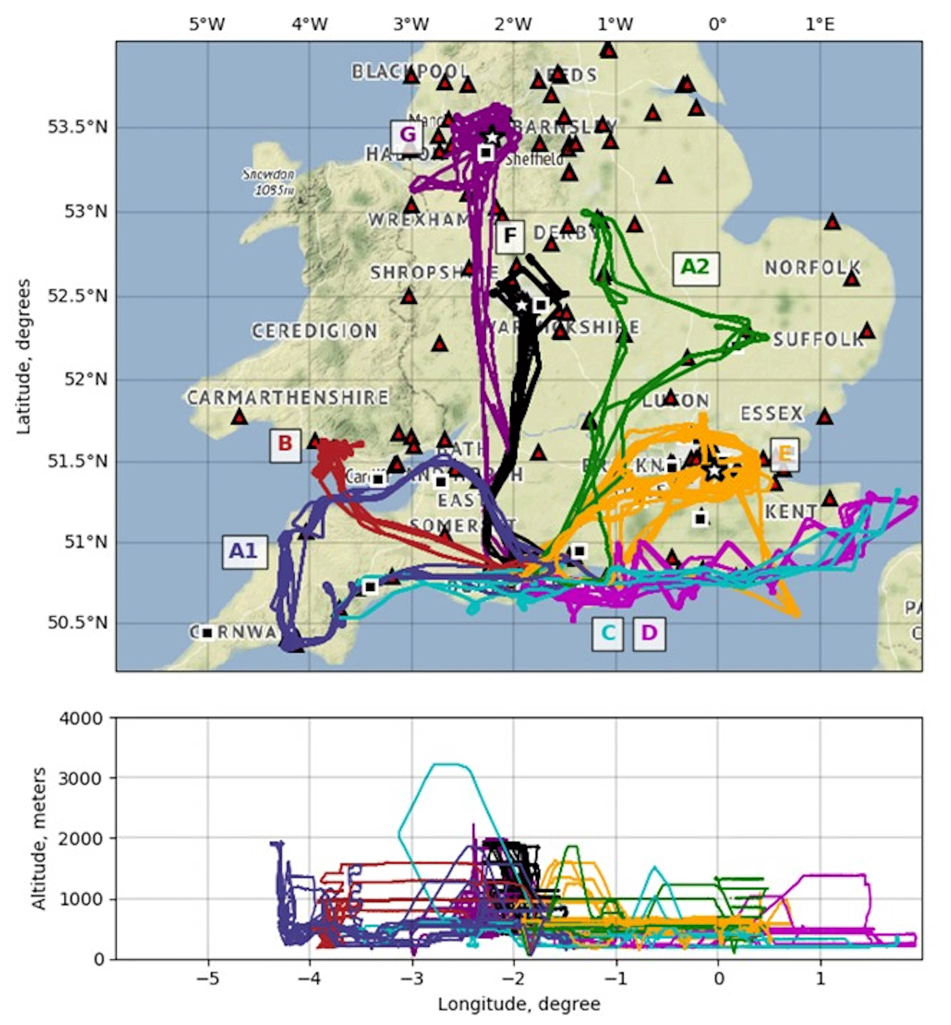
Figure 7Horizontal (top) and vertical (bottom) spatial coverage of 63 MOASA Clean Air flights from 27 July 2019 (flight M247) to 11 April 2022 (flight M326). AURN sites are shown as triangles, airports as squares and stars as ground-based supersites in Birmingham, Manchester and London. The annotations relate to the sortie type detailed in Fig. 8, where A1 and A2 are ground network surveys, B high-density plume mapping flights, C south coast surveys, D coastal transition surveys, E London City Surveys, and F and G the Birmingham and Manchester IOP flights, respectively. Map by Stamen Design, under CC BY 3.0. Data by OpenStreetMap, under ODbL.
Table 2MOASA Clean Air flights by sortie. The numbers in brackets indicate the number of straight and level transects used to derive the index of refraction for PM2.5 (where applicable) and (from flights M247 to M302) the analysis in Sect. 4.1. “n/a” indicates that no runs were used in forward analysis. London flights which include a central overpass are postfixed with an asterisk. Flights with limited data are postfixed with a double asterisk. London flights during the summer and winter IOPs are also postfixed with superscript “iop”. London flights with no NO2 data or O3 data are postfixed “NO2” or “O3” (applicable to Sect. 4.4).
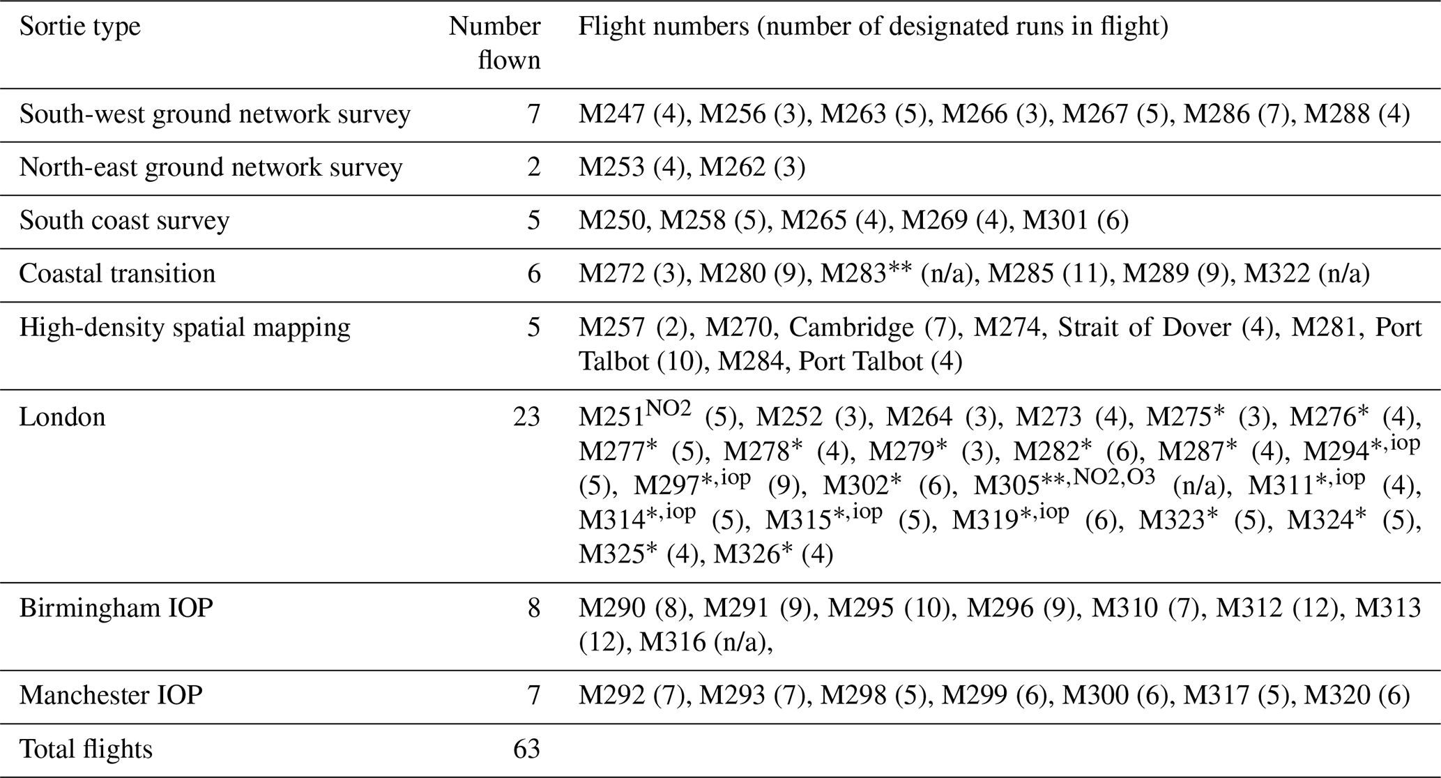
A total of 63 flight sorties were flown between July 2019 and April 2022, comprising over 150 h of atmospheric sampling. Flight details are summarised in Table 2, and Fig. 7 shows horizontal and vertical spatial coverage of flights over the Clean Air campaign.
In terms of meteorology, conditions representative of both the general background environment and elevated pollution events have been targeted. As the southern United Kingdom has a maritime climate, with the frequent passage of mobile low-pressure systems from the North Atlantic, conditions in the operating area are not always conducive to the build-up of pollution. For the targeting of elevated pollution conditions, synoptic high-pressure conditions with light winds and little cloud and precipitation are favoured. Strong sunshine and elevated temperatures are also conducive to the production and build-up of pollutants such as ozone, and as such, high pollution events tend to be more frequent and severe in the summer (Savage et al., 2013).
3.1 Ground network survey
Ground network survey sorties describe two flight patterns that sample both rural and urban background regional pollution at various altitudes. One flight pattern is focused on the south-western United Kingdom (Fig. 8a1) and the other on the eastern United Kingdom (Fig. 8a2). A particular feature of these sorties is that they overfly a number of AURN ground sites, allowing pollutant concentrations at the surface to be compared to those aloft. Characterisation of pollution at regional scales is important for air quality model evaluation, particularly for models operating at coarse resolutions such as AQUM, which encompass point source emissions data but cannot accurately represent them in terms of location and concentration.
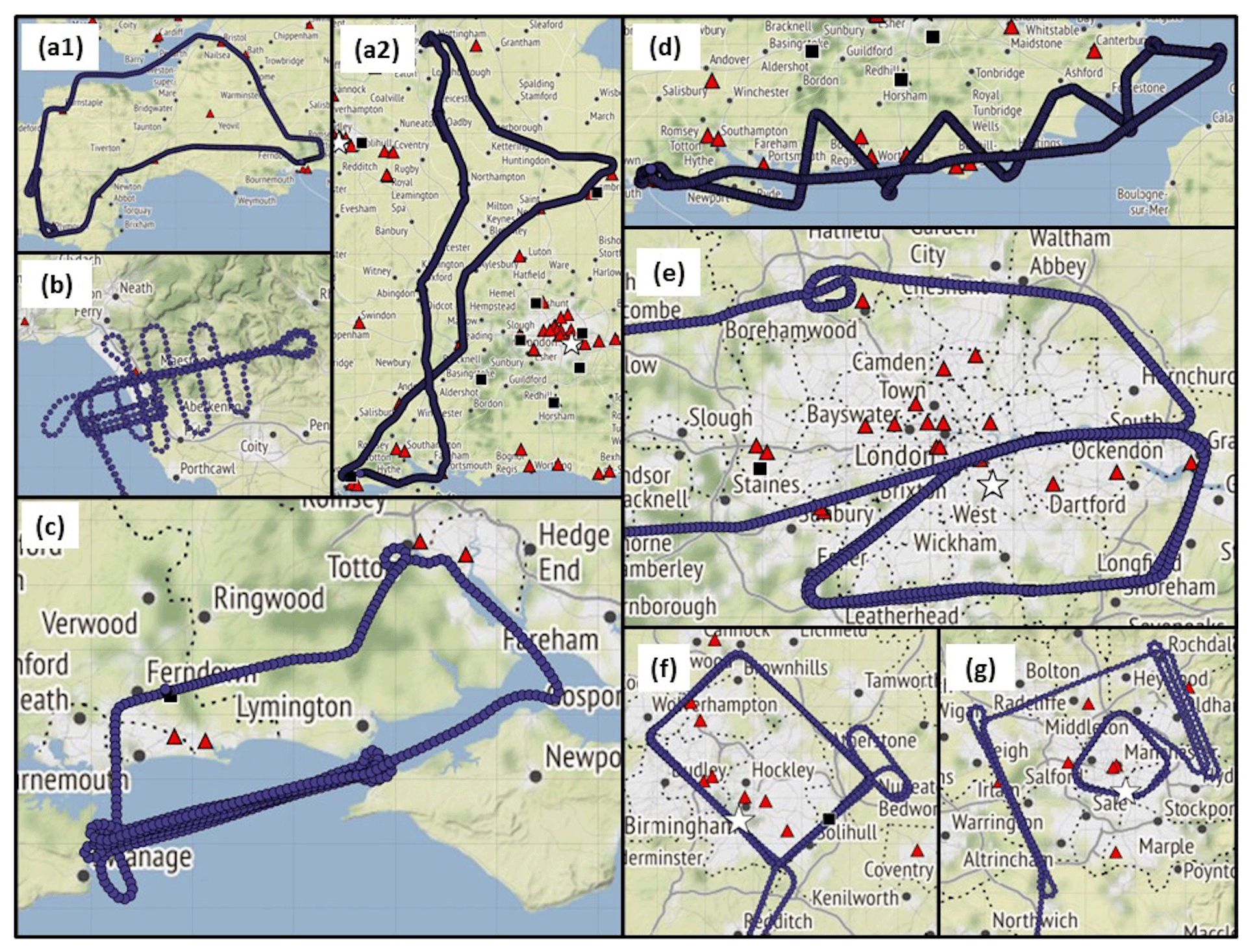
Figure 8Aircraft flight tracks for a typical (a) ground network survey over the south-west (a1) and east (a2), during M288 and M262 on 19 May 2021 and 10 January 2020, respectively, (b) high-density vertical mapping over Port Talbot, southern Wales, during M284 on 24 March 2021, (c) south coast survey flight, during M301 on 27 July 2021, with focus on overpasses of the Solent and Southampton waters, (d) coastal transition flight, during M285 on 30 March 2021, (e) London city survey flight IOP, M297 on 2 July 2021. (f) Birmingham IOP flight (left), during M296 on 1 July 2021, and (g) a typical Manchester IOP flight, during M300 on 20 July 2021. AURN sites are shown as triangles, airports as squares and stars are ground-based supersites in Birmingham, Manchester and London. The geographical location of each sortie is shown in Fig. 7. Map tiles by Stamen Design, under CC BY 3.0. Data by OpenStreetMap, under ODbL.
3.2 High-density plume mapping
High-density plume mapping flights (Fig. 8b) use intensive model grid-box scale sampling to allow for assessment of the (often subgrid in models) scale of pollutant variability in a high-pollution region. Repeated runs upwind, downwind and within the plume are performed at a range of altitudes. This sortie has primarily been flown over Port Talbot in southern Wales, a heavily industrialised area and AQUM pollution hotspot, but has also been flown once north of Cambridge (eastern United Kingdom). In that case, horizontal transects sampling the plume at multiple altitudes downwind of the city were conducted.
3.3 South coast survey
South coast surveys were flown onshore and offshore along the south coast of the United Kingdom, typically from Dartmoor National Park in the western United Kingdom to Eastbourne in the east (Fig. 8c). These surveys have been flown under background and polluted southerly flows to characterise transboundary and long-range transport of pollutants from continental Europe. In late 2019, a persistent emissions hotspot (primarily PM2.5 and SO2) was seen in the AQUM forecasts, potentially originating from ships in Southampton Docks. Therefore, from late 2019 onwards, overflights of the Solent and Southampton waters were added to the stock sortie.
3.4 Coastal transition survey
The coastal transition sortie (Fig. 8d) also operates along the south coast of the United Kingdom. The primary distinction from the south coast survey was a zigzag manoeuvre whereby observations across the land-to-sea transition are repeatedly sampled. The objective for this sortie is to obtain data for benchmarking model performance across the land–sea interface, where strong gradients in humidity and temperature can impact forecast pollution fields. In later flights, these surveys have also been extended eastwards to encompass the Strait of Dover to allow sampling of pollutants transported from industrial activities around the Dunkirk region of northern France, which is another emissions hotspot that can lead to strong pollutant transport over the United Kingdom when meteorological conditions permit.
3.5 London city survey
Circumnavigational flights of London (Fig. 8e) were performed during high- and low-pollutant loadings to characterise city scale emission and dispersion of pollutants from the heavily populated, commercial and industrial Greater London area. Busy air space and air traffic control due to the close proximity to major airports (Gatwick, London City, Heathrow) restrict the operational area of the MOASA. Broadly, following a short transit to Reading, the sortie takes the MOASA clockwise following the M25 London orbital motorway, which encircles Greater London. Missed approaches are frequently performed at Elstree airfield to the north and Biggin Hill airfield to the south-east.
A substantial decrease in air traffic during the COVID-19 pandemic provided a unique opportunity to fly at low level (approx. 1000 ft = 300 m) over central London. This central city sampling was added to the stock sortie in November 2020 and became the primary sortie for flights during the COVID-19 pandemic. The central London overpass follows the river Thames to approximately 0.087∘ W, where it deviates south-westerly to comply with air traffic control restrictions. During later flights, north–south and/or east–west transects were also completed to observe the urban heat island effect on boundary layer height. During the summer and winter IOP's MOASA observations were also made close to the surface air quality IOP supersite (stars, Fig. 8e).
3.6 Birmingham and Manchester IOP
During the summer and winter IOP's MOASA observations were also made over Birmingham (Fig. 8f) and Manchester (Fig. 8g). These city scale sorties were tailored to best suit meteorological conditions on the flight day; they typically involved circumnavigational orbits or box patterns over the cities at altitudes ranging from approximately 0.3 to 0.9 km and/or runs north–south, upwind and downwind of the city and the supersite. Passes directly overhead of the Birmingham and Manchester ground supersites (stars, Fig. 8f and g) were made at each altitude, when possible. During the IOPs, MOASA operated both in the morning and late afternoon, allowing observation of the build-up of regional-scale pollutants over the day.
3.7 The measurement database
Datasets obtained during the MOASA Clean Air project are openly available from the Centre for Environmental Data Archive (CEDA) “MOASA Clean Air Project: airborne atmospheric measurements collection” repository (DOI: https://doi.org/10.5285/0aa1ec0cf18e4065bdae8ae39260fe7d, Met Office and Mynard, 2023).
Data files are NetCDF format and contain observations of NO2 (ppbv, 1 Hz), ozone (ppbv, 0.5 Hz), SO2 (ppbv, 1 Hz), light scattering (Mm−1, 1 Hz), light absorption (Mm−1, 1 Hz), particle counts (number, 1 Hz), particle concentration (cm3, 1 Hz), calibrated, IOR-corrected particle mass (µg m−3 per bin, 1 Hz) including PM2.5 (µg m−3, 1 Hz). Data files also contain the meteorological parameters ambient temperature (∘C), relative humidity (%), pressure (hPa), wind speed (m s−1) and wind direction (∘), all at 1 Hz. Each instrument parameter is presented as a time synchronised, three-dimensionally geo-located time series, with calibrations and corrections applied (where applicable). Each instrument parameter has a standard name, long name, unit and measurement frequency (compliant with Climate and Forecast (CF) naming conventions where possible). Some, but not all, also have a comment, minimum and maximum limits, and/or a positive attribute. Each variable has the coordinates of time, latitude, longitude and altitude. Measurements from all instruments are reported at ambient pressure and temperature.
To ensure optimal traceability and transparency of data, comprehensive metadata are included in the NetCDF, which details any calibration constants and/or corrections applied to data alongside general information about the data, such as contacts, abbreviations and references. Where possible, data are range checked to ensure observations fall inside the recommended operational limits of the instrument, and outliers to these limits are flagged. The standard flag name is the parameter name, postfixed with “_flag”. The three flag values are 0 = good_data, 1 = outside_ valid_ranges, and 2 = sensor_nonfunctional. Where a flag is available, the valid ranges are given in the variable metadata. Each flag parameter has standard name, frequency, flag value and flag meaning attributes. Housekeeping variable flags are carried forward to the primary variables; primary variable flags are carried forward to secondary variables. The configuration file used to process each flight data is available alongside the NetCDF as a text file and provides the range check limits and the source of these limits. Records of all work done on the instruments (calibrations, cleaning, and maintenance) are digitally recorded and available on request by contacting the author.
This section provides a limited number of case studies applying the MOASA dataset to different scientific applications. These examples are intended to showcase different uses of the database and are not intended as comprehensive analyses in their own right. We present (i) a statistical analysis of the scales of pollutant variability observed across the MOASA air quality dataset, (ii) an introduction to the vertical structure of pollutants by comparing ground-based observations to airborne observations from repeated flight patterns over Greater London and (iii) example use of the dataset for evaluation of a regional air quality modelling system (AQUM).
4.1 The spatial scales of pollutant variability
The evaluation of limited-resolution regional air quality models (such as AQUM with a 12 km grid length) using high-resolution in situ surface or airborne data is complicated by the differences in spatial scale between the two (Qian et al., 2010). While instrumentation may be capable of measurements at high precision and accuracy, these uncertainty metrics often do not determine the degree to which models and observations should be expected to agree. In many cases the magnitude of natural pollutant variability at scales that are subgrid for models provides an important additional consideration. Quantifying subgrid-scale pollutant variability is also important for wider applications beyond model evaluation, such as pollutant exposure studies (e.g. Denby et al., 2011) and in understanding satellite-derived data (e.g. Tang et al., 2021). With this in mind, in this section we use the MOASA Clean Air database to assess how observed pollutant variability changes, on average, as a function of length scale, and how this variability compares to fundamental instrument measurement precision. As with each analysis presented in this section, the intention is to provide insight into potential application areas for the MOASA dataset rather than provide a comprehensive study.
High-temporal-resolution datasets corresponding to each straight and level run formed the basis for the analysis. An example of a straight and level run is shown in Fig. 9, which, notably, shows that SO2 data were generally below the sensitivity of the instrument except during exceedance events. Measured values in each dataset were split into groups of equal size, with sizes corresponding to equivalent ground distances (dint) ranging from 0.42 to 17 km, in 0.085 km (1 s) intervals (where a true airspeed of 85 m s−1 is assumed to be equivalent to 0.085 km s−1 straight-line distance at ground level). The variability observed at each of these length scales was calculated by first calculating the standard deviation (σ) of points within each group of data, before calculating the mean deviation across all groups in the transect.
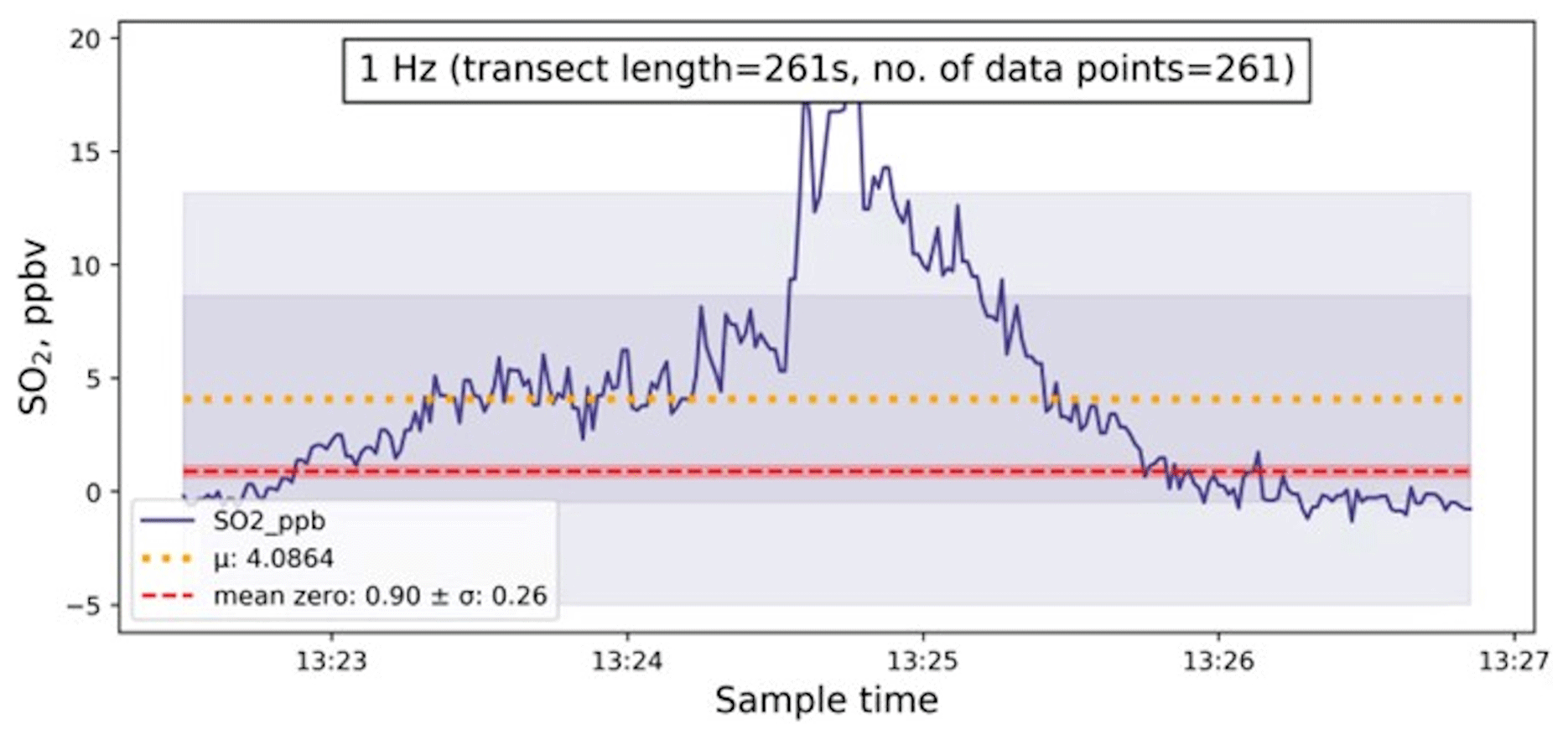
Figure 9SO2 time series from 13:22:30–13:26:50 UTC during high-density mapping flight M284. The solid blue line is SO2 concentration (in ppb), with the mean shown as the horizontal dotted line, with 1 and 2 standard deviations as the shaded grey areas. The mean SO2 zero (0.9 ppb) is the dashed red line, with red shading showing 1 standard deviation of the mean.
The variability observed in a given transect depends on a range of factors and will clearly change on a case-by-case basis. Despite this, it is also useful to examine how average, subgrid variability changes as a function of length scale (e.g. Tang et al., 2021, and references therein). This has been investigated here by using averaging data from all MOASA SLRs, over 63 flights between July 2019 and April 2022 (322 SLRs representing 1952 min of sampling). The number of SLRs per flight varies depending on the type of sortie flown, with a minimum of 2 and a maximum of 11 (see Table 2). The minimum permissible SLR length was capped at 3 min to ensure adequate counting statistics. We focus here on measurements of relative humidity, NO2, SO2 and total particle number concentration. The results are presented in Fig. 10 as probability density functions that indicate the range of variability observed at dint of 0.42, 0.85, 2.55, 5.10, 12.07 and 15.04 km.
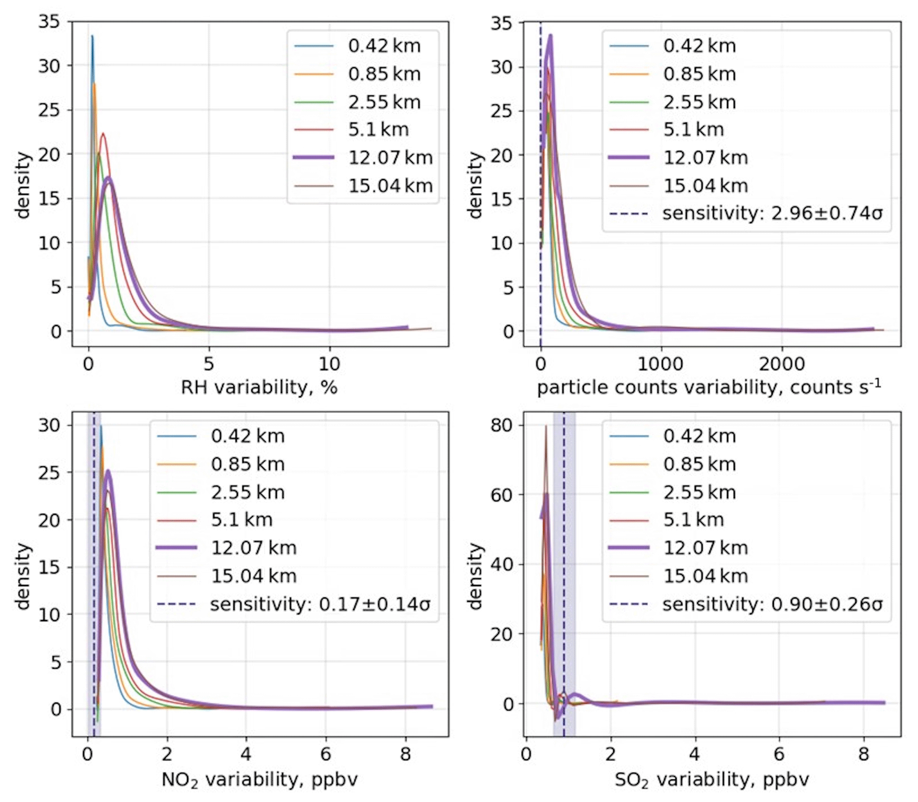
Figure 10Density distributions of RH, particle counts, NO2 and SO2 variability, for dint = 0.42, 0.85, 2.55, 5.10, 12.07 and 15.04 km, for 322 straight and level runs over 63 flights of the MOASA Clean Air campaign. Vertical dashed lines show the instrument sensitivity ±1 standard deviation.
Of particular note, it is clear that measured variability in SO2 was generally close to or below the noise limit of the MOASA instrumentation; thus instrument performance dominates not only SO2 background data (as seen in Fig. 9) but also observed SO2 variability in the MOASA database. For RH, NO2 and particle counts, natural variability is generally well sampled by the MOASA instrumentation. It is interesting to note how the peak position and width of the distributions changes upon moving to progressively longer sampling scales. Changes are particularly marked for relative humidity and somewhat less so for NO2 and particulate counts. Focusing on the 12 km AQUM grid length as an example, > 99 % of NO2 variability observed over the campaign is above instrument noise. This indicates that a significant amount of the variability in the NO2 dataset can be interpreted as real pollutant variability that could be used to help bound model parameterisations of subgrid variability, evaluate the accuracy of exposure estimates in air quality models, as discussed in Denby et al. (2011), and facilitate estimations of sampling uncertainties for satellite product validation, which has historically been limited by the availability of such in situ measurements (Tang et al., 2021).
4.2 Ground-based and airborne observation comparison using long-term observations over London
To enable meaningful comparison of airborne and ground-based observations during model verification, the relationship between observation methods must first be understood. To achieve this understanding, in this section, a comparison of airborne and ground-based observational data is presented.
The ground-based observations consist of OSCA mast and AURN data. AURN consists of around 70 sites in rural, remote, urban background and suburban settings, providing hourly measurements of NOx, SO2, O3, carbon monoxide (CO), PM2.5 and coarse particulate matter (PM10) (Environment Agency, 2022), although not all species are measured at all sites. For this paper, we only consider background AURN sites applicable to regional air quality models such as AQUM (Neal et al., 2014).
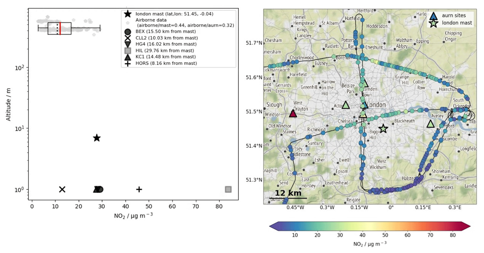
Figure 11Flight M325 on 24 March 2022 from 12:09:25 to 13:46:01 UTC. Left: altitude profile, where airborne observations of NO2 within Greater London are shown in grey, and the boxplot represents the inter-quartile range, the data range (whiskers), the median (vertical dashed black line) and mean (vertical red solid line) of these data. The London IOP supersite is shown as a black star, and AURN ground sites within the region are shown as various markers (see key). Ratios of airborne : mast (0.44) and airborne : aurn (0.32) are calculated as the ratio of mean airborne observations to the mast, and to the mean of all individual ground-based sites, respectively. Right: track of aircraft coloured by NO2 concentration (representative of the range of the airborne data in the profile plot), with mast-based (star) and ground-based (triangles) NO2 observations. Map by Stamen Design, under CC BY 3.0. Data by OpenStreetMap, under ODbL.
For the comparison, first, the vertical structure of NO2, PM2.5, SO2 and O3 were plotted as altitude profiles of airborne data alongside all available ground data within Greater London (longitudes from −0.60 to 0.40, latitudes from 51.23 to 51.80). The agreement (ratio) between airborne and ground-based observations was moderately low for all species for most flights, likely due to large variation between ground sites, in terms of site proximity to the airborne data and variation in concentration due to proximity to emission sources. An example of the vertical and horizonal spatial variation of airborne and ground-based observations for NO2 during flight M325 over Greater London is shown in Fig. 11. Here, the 84 µg m−3 NO2 observed at the HIL AURN site (Fig. 11 left: grey square and right: red triangle) is significantly higher than both other ground sites in the region and the airborne data (boxplot whiskers in Fig. 11 left and track colour in Fig. 11 right). This skews the airborne : ground ratio to 0.32 (the ratio discounting this site is 0.48). This suggests a region-wide observational comparison is insufficient in determining whether the airborne data can be meaningfully compared to the ground data and is an inefficient metric when using these observations for model evaluation, where models can have significantly higher resolution. As shown in Sect. 4.1, MOASA instrument precision did not limit the ability to sample the natural pollutant variability at spatial scales of 0.42 km, important for representing the magnitude of natural pollutant variability at scales that are subgrid for models.
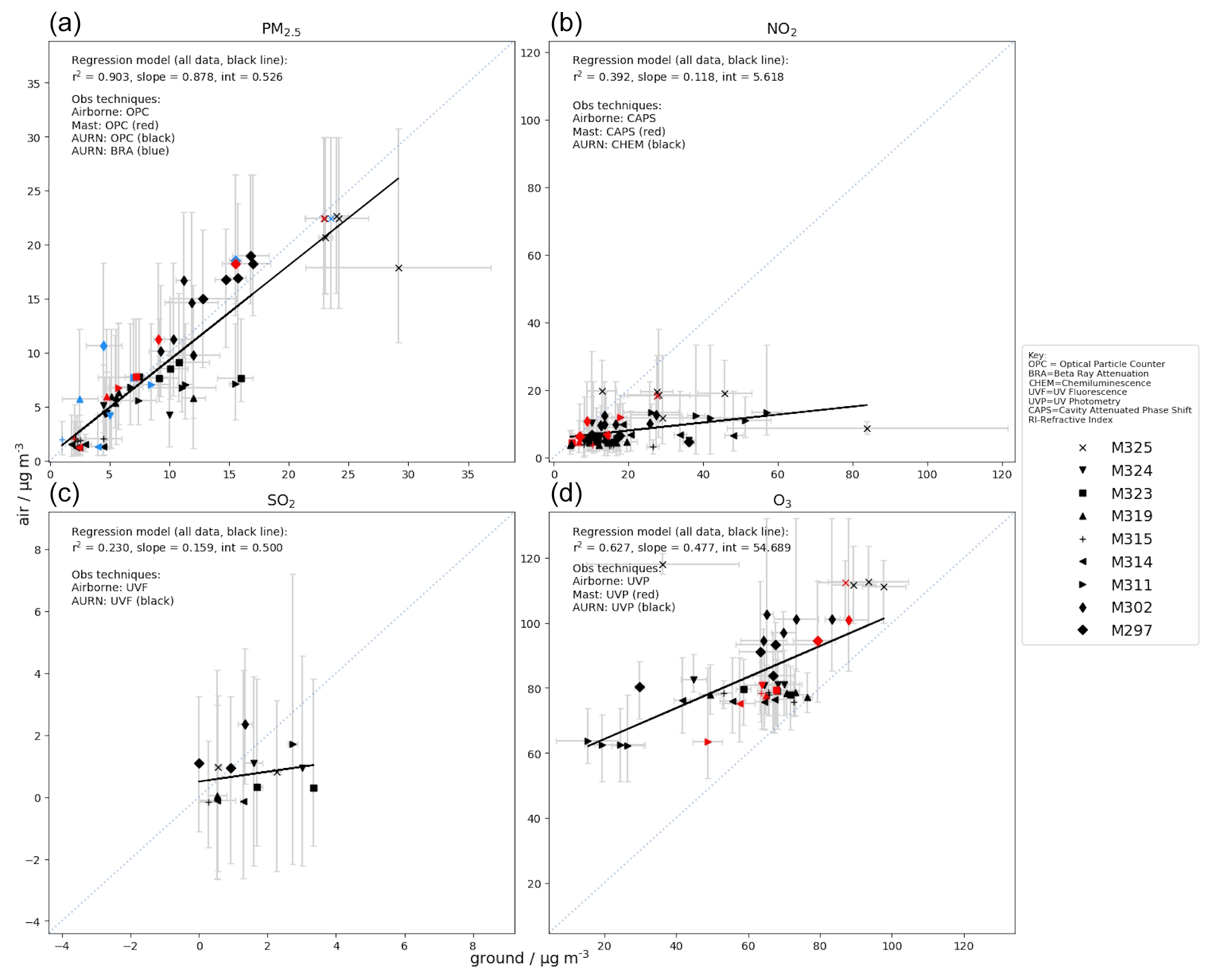
Figure 12Average airborne observations within a 12 km radius of ground site, against local ground site average, for PM2.5 (a), NO2 (b), SO2 (c) and O3 (d), for all available London IOP flights. Comparisons against OSCA mast data are shown in red and against AURN ground sites in black. For PM2.5, blue markers identify those AURN sites that employ beta ray attenuation technique (black employs an optical particle counter with conversion to mass technique) . Linear regression between airborne and ground- and mast-based data is shown in black. Error bars (grey) show the range of data; the 1–2–1 line, representative of a perfect linear relationship, is shown as a dotted grey line.
To minimise the effects of the horizontal spatial variation of concentrations and utilise the high spatial resolution of the airborne data, the average airborne observation within a 12 km radius (the AQUM grid length) of each ground site was calculated. For each species, these airborne averages were plotted against the local ground-based average observation, for each ground site, for each IOP flight. Linear regression was then modelled for each species and site. The result of this approach is shown in Fig. 12 for the Greater London area.
4.2.1 PM2.5
Linear regression of airborne vs. ground-based observations of PM2.5 inside the London area suggests very good agreement between the two datasets, with r2 of 0.90. The agreement between observations suggests a well-mixed atmosphere, with little gradient in PM2.5 throughout the column. The majority of observations are obtained using the same measurement technique (optical particle counter with conversion to mass concentration) with just one AURN site (London Westminster) using a beta ray attenuation (BRA) technique. As discussed in Sect. 2.8, airborne PM2.5 is derived from size distributions that are refractive index corrected on a per-flight basis and a density of 1.64 g cm−3. For the majority of AURN ground sites, both refractive index and density are derived internally to the instrument, using 24 h average gravimetric data. This comparison suggests these correction methods yield agreeable results. The parity of the BRA observations with the majority equivalent method provides further reassurance that, for this study, all observations of PM2.5 are comparable, regardless of observation technique employed.
4.2.2 SO2
Due to limited AURN sites that observe SO2, as well as low concentrations of SO2, which generally do not exceed the uncertainty thresholds of the airborne instrumentation, there are insufficient observations to explore agreement between the observational platforms, which both employ a UV fluorescence technique. However, at the low concentrations shown and the site data available, the observations show reasonable agreement. That both airborne and ground-based observations are made using the same measurement technique provides further confidence that the observations are comparable.
4.2.3 NO2 and O3
A weak positive agreement is shown for NO2 where r2 = 0.40, suggesting a more variable relationship between airborne and ground-based observations. The model shows systematically lower NO2 observations aloft at most sites, which diverge further away from unity with an increase in concentration. A moderate, positive agreement is seen for O3, where r2 = 0.63. Contrary to the NO2 model, the agreement between observations aloft and at the ground moves towards unity at higher concentrations, and systemically higher observations are seen aloft at all sites. Flight dates for observations at lower O3 concentration were in winter, whereas flight dates for observations of the highest concentrations – where agreement is strongest – are in the summer and spring months.
All observations of O3 use ultraviolet photometry, whereas for NO2, observations aloft and at the OSCA mast sites use cavity attenuated phase shift spectroscopy, and the AURN sites employ chemiluminescence. There are numerous possible explanations as to why we might not expect observations at the ground and aloft to agree well for these reactive chemical species, including instrument bias (particularly for NO2, which employs different observation techniques), complex chemistry and mixing throughout the column.
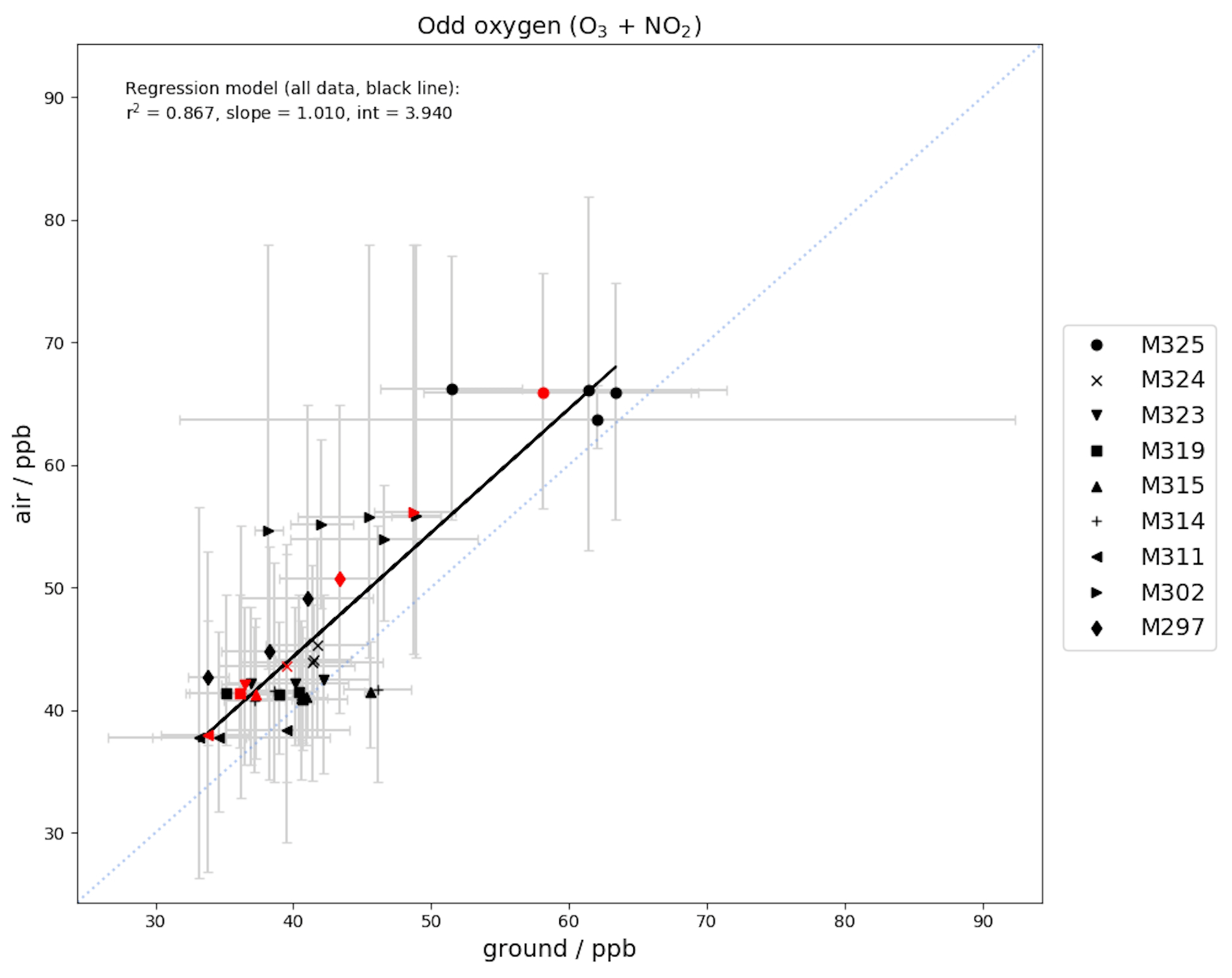
Figure 13Odd oxygen, calculated from average airborne observations of O3 + NO2 (in ppb) within a 12 km radius of ground site, against local ground site average O3 + NO2 (in ppb), for all available London flights. Comparisons against OSCA mast data are shown in red; comparisons against AURN ground sites are shown in black. Linear regression between airborne and ground- and mast-based data is shown as a black line. Error bars (grey) show the range of O3 + NO2 data; the 1–2–1 line, representative of a perfect linear relationship, is shown as a dotted grey line.
Assuming the simplest mechanism linking chemistry at the ground to that aloft, whereby NO emitted at the surface reacts with O3 via titration to form NO2 (NO + O3 ⇒ NO2 + O2), odd oxygen (Ox, in this case defined as the sum of O3 plus NO2; Bates and Jacob, 2019) is expected to be conserved throughout the atmospheric profile. Figure 13 shows a comparison of Ox observed at the surface versus aloft for the London sites, which yields a regression model gradient of near 1. These results – noting that this simple model neglects mixing, O3 production, deposition, and other loss mechanisms – are broadly consistent with chemistry via O3 titration being dominant for the cases observed here and indicate that the airborne air masses were coupled to the surface, conducive to the findings of the PM2.5 analysis. An r2 of 0.87 also provides confidence that the observations are comparable, regardless of observation technique employed.
4.3 Preliminary model evaluation
In this section we show examples from two flights illustrating how the MOASA Clean Air database can be used for model evaluation purposes. These flights are M270 high-density plume mapping on 15 September 2020, selected to measure the vertical distribution of pollutants in the lower atmosphere north of Cambridge (52.2053∘ N, 0.1218∘ E) and M296, a Birmingham city survey as part of the IOP on 1 July 2021. Meteorological conditions for the flights are summarised in Fig. 14. For M270, there were largely clear skies with light winds (< 10 m s−1) in the south-eastern United Kingdom where sampling was undertaken and high temperatures (National Meteorological Library, 2020), conducive to the accumulation of pollutants in the boundary layer. M296 was influenced by high pressure, light winds and thin, broken clouds.
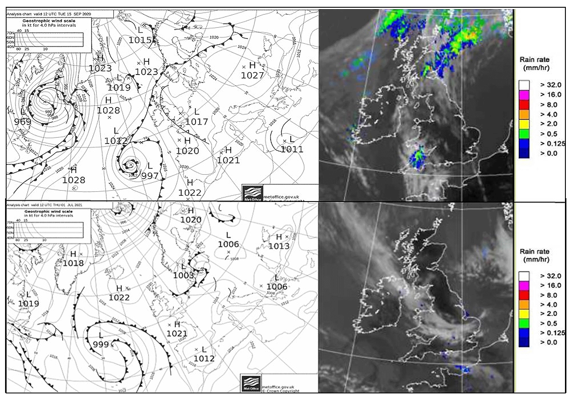
Figure 14Met Office synoptic chart and combined infrared and rain-radar images for 12:00 UTC 15 September 2020 (top) and 1 July 2021 (bottom) (National Meteorological Library, 2020).
Case studies of the flight days have been run using the AQUM UK domain model. This is the same model configuration used for the operational air quality forecasting, but for these case studies, no routine statistical post-processing (SPP, which uses surface level observations to apply corrections to the surface model level only) has been applied to the data. Given that this study focuses on those data above the surface level, the omission of the SPP has no impact on the evaluation. Each simulation has been run with a 7 d spin-up period. No adjustments have been made to the emissions used by the model to account for changes in activities during the COVID-19 restrictions. Model data points have been linearly interpolated using the time, latitude, longitude and altitude coordinates of the aircraft at 1 s frequency. The model and aircraft data along the flight tracks have then been averaged into 10 s, non-overlapping intervals.
4.3.1 Flight M270
In consonance with Savage et al. (2013), a large ozone bias is seen for flight M270 (Fig. 15a). The model data show a large overprediction when compared against the aircraft data at corresponding locations (mean model bias of 18.49 ppb). The bias is lowest near the surface and increases with altitude up to approximately 700–800 m, above which the bias decreases. The variability observed is poorly represented by the coarse-resolution model. Variation in the AQUM model data is largely caused by changing from one grid box to the other, and ozone shows a typically smooth gradient between model grid boxes. We note that in this case the stacked flight transects only cross a very small number of model cells (three or four) in the horizontal, which may be accountable for the low model variability seen here. Figure 16 shows the comparison between the model and aircraft NO2 data for vertically stacked transects for the same time period. The agreement is generally good (within ±2 ppbv) below 650 m altitude, but the model shows large underprediction above this altitude. Temperature and relative humidity profiles measured by the aircraft (not shown) suggest a boundary layer height of approximately 1100 m on this day, which corresponds with a decrease in observed NO2 concentration above this height. However, the average boundary layer height in the model for the observed area is approximately 620 m. This indicates a potential underprediction in boundary layer height that may be responsible for the poor predication of NO2 at elevated altitudes and elucidates the altitude dependence on the ozone model bias discussed above.
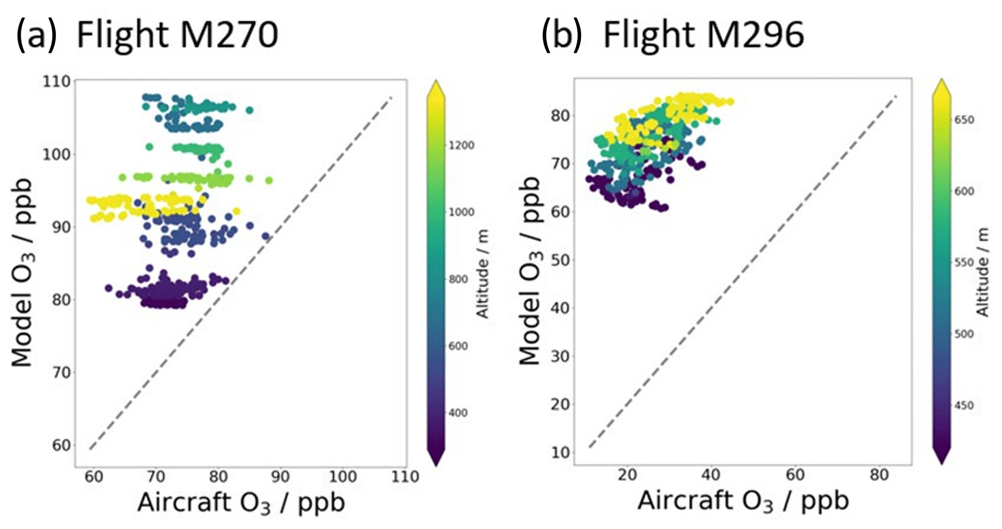
Figure 15Correlation of model and aircraft O3 concentrations. Data averaged over 10 s intervals. Markers coloured by altitude. Dashed grey line represents agreement between the two datasets. Data shown for (a) flight M270 on 15 September 2020, from 12:13:00 to 13:38:00 UTC (the duration of the stacked level runs north of Cambridge) and (b) flight M296 on 1 July 2021 from 11:23:00 to 12:52:00 UTC (the duration of the Birmingham city circuits).
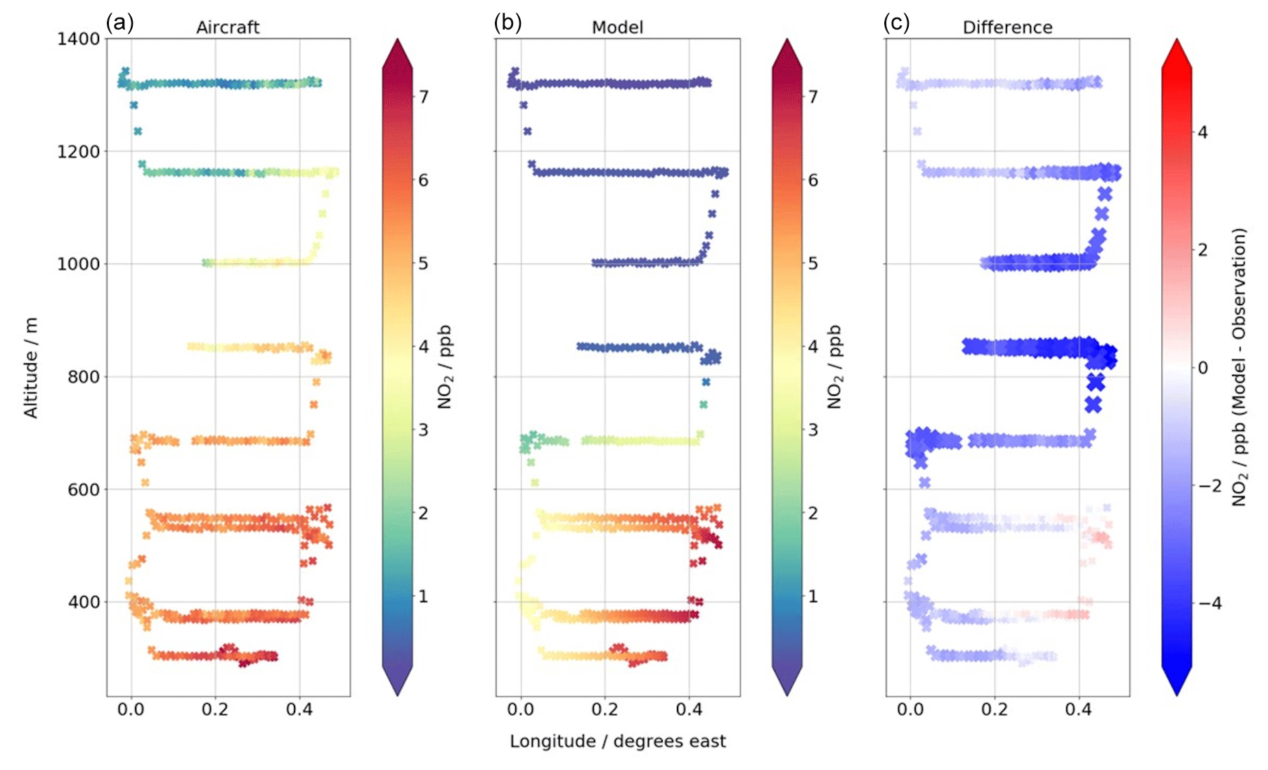
Figure 16Longitude–altitude plot of NO2 concentration for vertically stacked transects during flight M270 on 15 September 2020. Panel (a) shows the aircraft data, (b) the model data and (c) the difference between the model and aircraft, where opacity and thickness increase as the difference diverges away from zero. Data averaged over 10 s intervals.
4.3.2 Flight M296
A large positive model ozone bias is also seen for flight M296 (Fig. 15b) when compared against the aircraft data at corresponding locations (mean model bias of 48.93 ppb). Unlike flight M270, the bias appears relatively constant with altitude, likely due to the flight being solely inside the boundary layer. Also unlike flight M270, the observations and model show similar variability. This is likely due to the flight track crossing a larger number of model cells, which encompass more model predictions and may also be due to the model capturing more variability for this case.
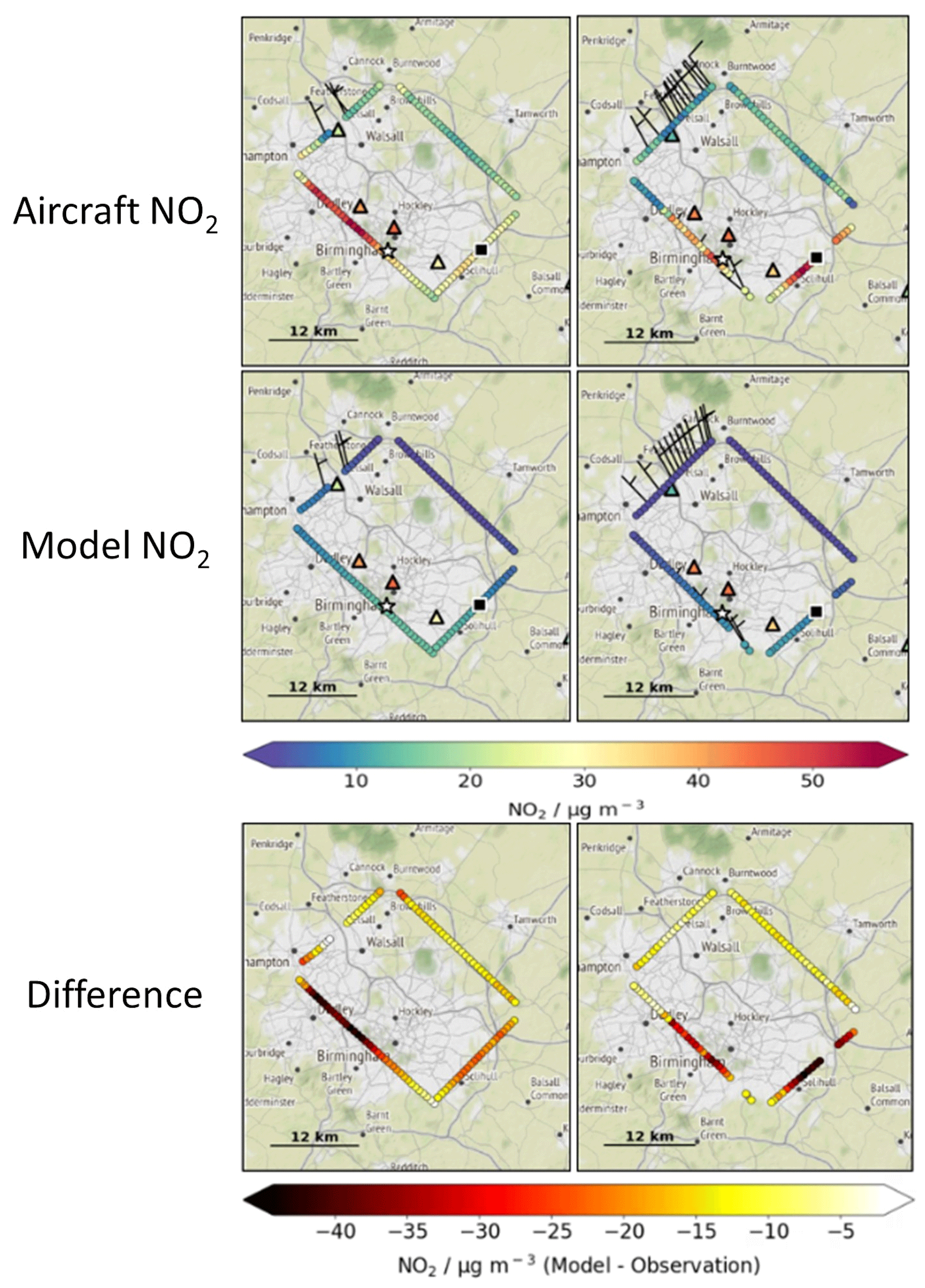
Figure 17Aircraft flight tracks coloured by NO2 concentration (µg m−3) for the first (left, 11:23 to 11:43 UTC) and fourth (right, 12:33 to 12:52 UTC) circuit, at altitudes of 423 and 657 m, respectively, around Birmingham during flight M296 on 1 July 2021. The top row shows the aircraft data. The middle row shows the model data. The bottom row shows the difference between the model and observations. Observation data are from straight and wing level transects, and all data are averaged over 10 s intervals. Wind barbs are only shown where the observed wind components exceed the measurement uncertainty. Data in triangles are the hourly surface level AURN NO2 concentration for the circuit. Stars and squares show the location of the Birmingham supersite and airport, respectively. Map tiles by Stamen Design, under CC BY 3.0. Data by OpenStreetMap, under ODbL.
Figure 17 shows model and observed NO2 concentration throughout the first and fourth stacked box patterns performed around Birmingham during M296. Strong variation is observed in NO2 concentration aloft of the city, including enhanced NO2 at all altitudes (maximum 55.70, 49.44, 56.31 and 54.06 µg m−3 NO2 for circuits 1–4, respectively; see Appendix D for circuits 2 and 3). The enhanced NO2 plume is seen above the western quadrant of the city during the lowest-altitude circuit (circuit 1, 423 m, 11:23 to 11:43 UTC) and moves south-east with increasing altitude, until the plume is observed primarily over the south-east quadrant of the city during the highest-altitude circuit (circuit 4, 657 m, 12:33 to 12:52 UTC). In contrast, observed O3 aloft (not shown) is inverse to the NO2 observations and shows a reduction of approx. 20–30 µg m−3 at the plume locations at all altitudes. Comparison of NO2 aloft with average surface level observations over the transect time (triangles, 1 h data frequency) shows similar concentrations. In consonance with AQUM, light north-westerly winds (0 < 5 kn) associated with the high-pressure system are observed in all circuits. These slack winds (equivalent to a maximum velocity south-eastward at 9.26 km h−1) likely pushed the plume (which is seen in the ground data to be present east of the flight track) south-eastward, accounting for the shift in the observed plume with altitude and time (approximately 1 h between the first and final circuits). The proximity of the plume to Birmingham airport is also of note in run 4. The AQUM model shows little variation and low NO2 concentration in comparison to both airborne and ground-based observations in all circuits above the city (maximum 14.44, 13.91, 11.43 and 10.33 µg m−3 NO2 for circuits 1–4, respectively, which decrease imperceptibly with altitude). A negative NO2 model bias is evident at the observed plume locations, with maximum differences of −44.26, −44.30, −49.22 and −49.79 µg m−3 NO2 for circuits 1–4, respectively. This model bias is expected to have been larger if the AQUM data were produced using emissions modified for the COVID-19 pandemic (Grange et al., 2021).
Given the flight track is mostly within just four model grid boxes, variation in NO2 concentration from point source emissions is not expected to be represented in fine detail in the model. As the observed peak in NO2 is located downwind of important sources (motorways and a heavily urbanised area) and given the dependence of surface concentrations of this primary pollutant on local emissions (Neal et al., 2017), the lack of enhanced NO2 at all levels of the model could be attributed to emissions being too low at the observed plume location.
A long-term, quality-assured dataset on the three-dimensional distribution of NO2, O3, SO2 and fine-mode PM2.5 aerosol, including optical absorption and scattering properties, has been collected over the United Kingdom using the instrumented Met Office Atmospheric Survey Aircraft from July 2019 to April 2022. Observations allow for the evaluation of regional air quality models such as AQUM. A description of the MOASA measurement platform and instrumentation is presented, along with details of flight plans, designed to allow repeatable, comparable observations of pollutants.
A total of 63 flight sorties, totalling over 150 h of sampling, were flown during the campaign. These flights include observations of city scale pollution over Birmingham and Manchester during two periods of intensive observations in June–July 2021 and January–February 2022, as well as long-term (2019 to 2022) observations over London, including central London overpasses (from October 2020).
Analysis of relative humidity, total particle counts and NO2 over the campaign shows that instrument precision did not limit the ability to sample the natural pollutant variability, at length scales down to 0.42 km. In contrast, SO2 variability is shown to be limited by instrument precision at all length scales. Comparison of airborne to ground-based observations generally shows good agreement between the observation platforms, regardless of observation technique. The overall strong correlation between airborne and ground-based PM2.5 (r2 of 0.9) implies that the observations are likely comparable when carried out within a well-mixed boundary layer. The low-sample, low-concentration SO2 observations analysed here also suggest that the observations are comparable. For NO2 and O3, chemical processing in the atmospheric column yields an intricate, poorly correlating relationship between airborne and ground-based observations. In contrast, odd oxygen (Ox = NO2 + O3) at the ground and aloft strongly agrees (r2 = 0.87, gradient = 1), suggesting that, for the cases analysed here, ozone titration played a dominant role in the chemistry of these species throughout the atmospheric column. A slight offset in the regression model indicates that O3 is higher aloft, suggesting processes unrepresented by this simple model (recalling the limitations noted in Sect. 4.2.3) may also be present.
Preliminary comparison of aircraft, ground-based and mast-based observations with AQUM data highlights the use of the database for air quality model evaluation work, to substantially augment sparse ground observations. Large ozone biases are seen for both flight M270 and M296, where the model data show large overpredictions when compared against the aircraft data at corresponding locations. The bias appears to be relatively consistent across the latitude and longitude ranges of the flights and does not show any particular correlation with location, although it appears to decrease with altitude in flight M270. Potential underprediction of model boundary layer height in flight M270 may be responsible for this altitude-dependent ozone model bias, as well as the poor predication of NO2 seen at elevated altitudes in the model. It is of note that the model biases seen are expected to have been larger if the AQUM data were produced using emissions modified for the COVID-19 pandemic (Grange et al., 2021). Variability in modelled ozone appears to be dependent on the number grid boxes encompassed by the flight track. It is expected that ozone concentration in higher-resolution models (> 12 km) will better match variation in the airborne observational data, as model resolution moves towards natural-scale variability. During M296, contrary to the model, enhanced concentration of NO2 is observed downwind of important sources. Observations aloft are in reasonable agreement with the available ground-based observations, suggesting the air mass aloft is coupled with the ground. Meteorological conditions are broadly consistent between the model and observations, which implies low emission estimates may be responsible for the negative NO2 model bias in this case. These example case studies provide handles for further investigation associated with biases in modelled O3 and NO2 concentrations, boundary layer height and representation of emissions in coarse-resolution models. We anticipate that the airborne dataset may also be useful for derivation of bias-correction factors that can be applied to model data during post-processing.
This paper serves as a reference for all future database users. The MOASA Clean Air database is comprised of quality-assured observations, presented in NetCDF format with robust metadata to ensure traceability and transparency of data. Data are openly available from the CEDA (MOASA Clean Air Project: airborne atmospheric measurements collection) repository (DOI: https://doi.org/10.5285/0aa1ec0cf18e4065bdae8ae39260fe7d, Met Office and Mynard, 2023).
The air quality box, as introduced in Sect. 2.1 and shown schematically in Fig. A1, houses the POPS and TAP instruments, as well as actuated valves and flow controllers which control the sample flow to instruments.
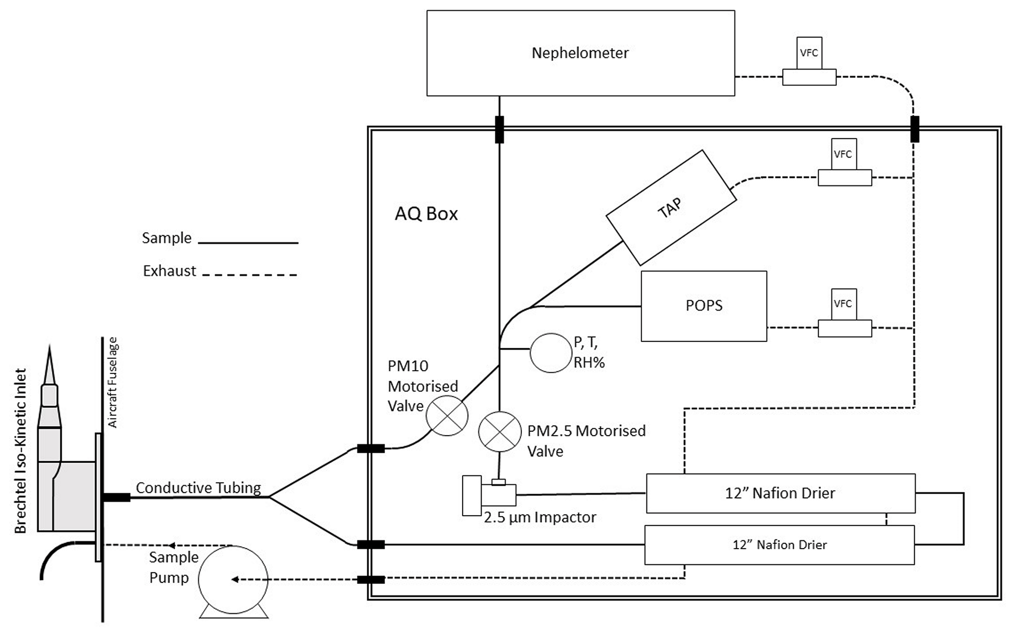
ω0nt is determined by calculating the average single-scattering albedo over the same flight transect as ω0psd. First, the Virkkula-corrected TAP (absorption) data are smoothed to a 10 s triangular window to match the Muller-corrected nephelometer (scattering) data. The scattering and absorption Ångström exponents (SAE and AAE, respectively), calculated as per Eq. (B1), were used to adjust the multi-wavelength nephelometer (λ = 635, 525 and 450 nm) and TAP (λ = 652, 528 and 467 nm) instruments to the POPS wavelength (λ = 405 nm) using Eq. (B2) (Perim De Faria et al., 2021). Uncertainties in derivation of AAE (from potential asynchronous sampling response times and flow rates) were reduced by applying maximum and minimum bounds estimated by considering the extremes of expected ambient AE values. Here, the AAE upper and lower bounds are 3 and 0.7, respectively. AAE is removed when raw red absorption < 1 Mm−1, and the AAE is set to 1.5 if the difference between absorption channels is < 1 Mm−1. For the SAE, upper and lower bounds are 2.5 and 0.5, respectively. SAE is removed when raw red absorption < 10 Mm−1, and the AAE is set to 0.5 if the difference between scattering channels is < 1 Mm−1. The data are then further averaged over 30 s to minimise variability from instrument noise and precision and any mismatch of data. To minimise uncertainties in wavelength correction using the Ångström exponents, ω0nt is derived from the blue wavelengths only, using Eq. (B3).
where AE is the Ångström exponent, AOC the aerosol optical coefficient (scattering or absorption), and λ1 and λ2 are wavelengths pairs.
where λ405 is the POPS wavelength (nm), λi is the wavelength of the given scattering or absorption coefficient and AE is the Ångström exponent.
where the bar indicates the 30 s rolling average, for scattering (scat) and absorption (abs) for the blue wavelength nephelometer and TAP channels, converted to POPS wavelength (λ405).
Determining ω0 using separate instruments with different uncertainties and principles can lead to potentially significant errors and biases (Perim De Faria et al., 2021). The uncertainty in the ω0nt calculations is related to the corresponding uncertainties in the scattering and absorption coefficients (Peers et al., 2019) measured by the nephelometer (4 % at 450 nm, 2 % at 525 nm and 5 % at 635 nm; Müller et al., 2011) and TAP (30 %; Ogren et al., 2017). These total measurement uncertainties are propagated according to Appendix A of Perim De Faria et al. (2021) to give an uncertainty for ω0nt (Eq. B4).
where σsc is independent scattering and σa is independent absorption coefficients.
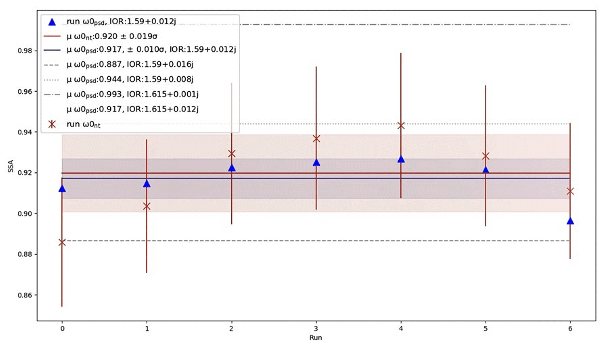
Figure B1Empirically derived nephelometer and TAP single-scattering albedo (ω0nt, red, crosses) and theoretically derived particle size distribution single-scattering albedo (ω0psd, blue, triangles) for seven straight and level runs for flight M270 on 15 September 2021 north of Cambridge. Flight mean ω0nt and ω0psd with 1σ variance (solid lines and shaded areas in red and blue, respectively) are shown. Also shown are the mean ω0psd derived using particle size distributions (PSDs) corrected with the IOR, which yielded ω0psd that closely matches the minimum ω0nt (run 0, dashed grey line) and maximum ω0nt (run 4, dotted grey line), where PSD IOR = 1.59 + 0.016j and 1.59 + 0.008j, respectively. The mean ω0psd derived using uncorrected (PSL-calibrant IOR = 1.615 + 0.001j) PSDs is also shown (grey dot–dash line). The mean ω0psd derived using a real component of 1.615 and imaginary component of the retrieved IOR (0.12) is detailed in the legend (line not shown).
ω0 is not very sensitive to the real part of the index of refraction, and as such the real part of the estimated index of refraction is not very well constrained (Peers et al., 2019). Figure B1 shows ω0psd derived using IOR = 1.615 + 0.012j and IOR = 1.59 + 0.012j, which both yield a mean ω0psd of 0.917. As such, we use a real aspect of 1.59 as derived by McMeeking et al. (2012) during their airborne measurement campaign over London, United Kingdom, in 2009. Where insufficient data are available to enable calculation of the ω0 and thus IOR, an IOR of 1.59 + 0.0j is adopted. The uncertainties associated with applying a flight-mean IOR are investigated in more depth in the following case study.
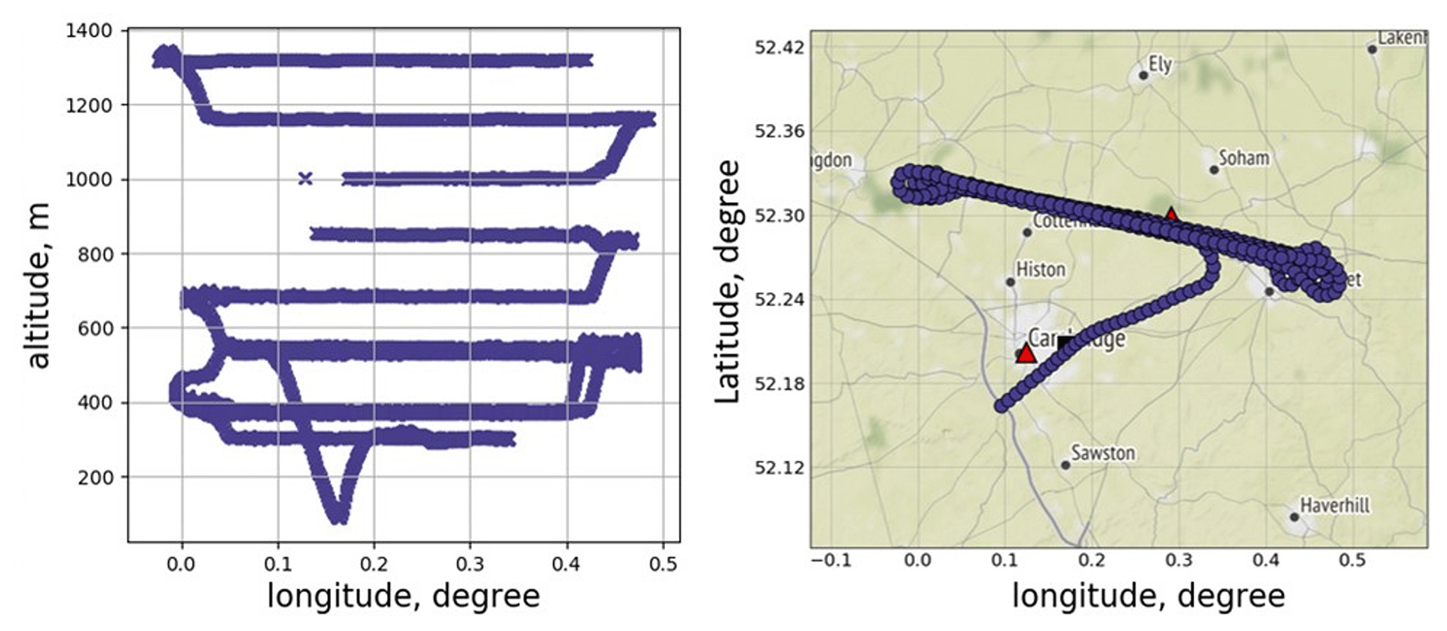
Figure B2MOASA flight track for M270 north of Cambridge on 15 September 2020 in the vertical (left) and horizontal (right). Triangles are AURN sites; the square is Cambridge Airport. Map tile by Stamen Design, under CC BY 3.0. Data by OpenStreetMap, under ODbL.
Table B1Mean altitude and single-scattering albedo derived using the nephelometer and TAP (ω0nt) and particle size distributions (ω0psd) for seven runs during flight M270 on 15 September 2020.
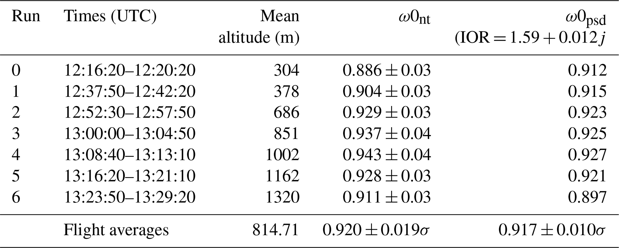
Section 2.7 describes the processing applied to particle sizing measurements to account for sizing errors caused by differences in the IOR between the calibrant and ambient particles. The method applies corrections based on the assumption of a single ambient IOR per flight, which was derived via an iterative process based on achieving closure with independent observations of particles single-scattering albedo. In this section we undertake a sensitivity study to evaluate the magnitude of error arising from the assumption of a flight-mean IOR, based on variability observed during an example flight: M270, a high-density plume mapping sortie north of Cambridge, where a sequence of straight and level runs at altitudes from 0.30 to 1.32 km were performed (Fig. B2 and Table B1). The wide range of altitudes over a single flight allows examination of the impact of a potentially changing air mass with altitude on derivation of a flight mean IOR. Refer to Sect. 4.3 for a description of meteorological conditions for this flight.
The range of measured single-scattering albedos, ω0nt, during flight M270 varied throughout the boundary layer (0.886 to 0.944, Fig. B1 red crosses) and yielded a flight mean ω0nt = 0.921 ± 0.019σ (Fig. B1, red line). These values fall within the range of single-scattering albedos observed by McMeeking et al. (2011) during airborne observations over London (typically from 0.85 in urban plumes to 0.95 in regional pollution and background aerosol).
A flight mean ω0psd = 0.917 ± 0.10σ (Fig. B1, blue line) was calculated using a particle size distribution (PSD) corrected with an optimally derived IOR = 1.59 + 0.12j (herein referred to as IORDER). To examine sensitivity in particle sizing due to variability in observed ω0 throughout the column, we also undertook PSD corrections based on achieving closure between ω0psd and the maximum observed ω0nt (IORMAX, 1.59 + 0.008j), minimum ω0nt (IORMIN, 1.59 + 0.016j) and an uncorrected PSD (which retains the calibrant (PSL) IOR; IORPSL, 1.615 + 0.001j), shown as the dotted grey, dashed and dash–dot lines, respectively, in Fig. B1.
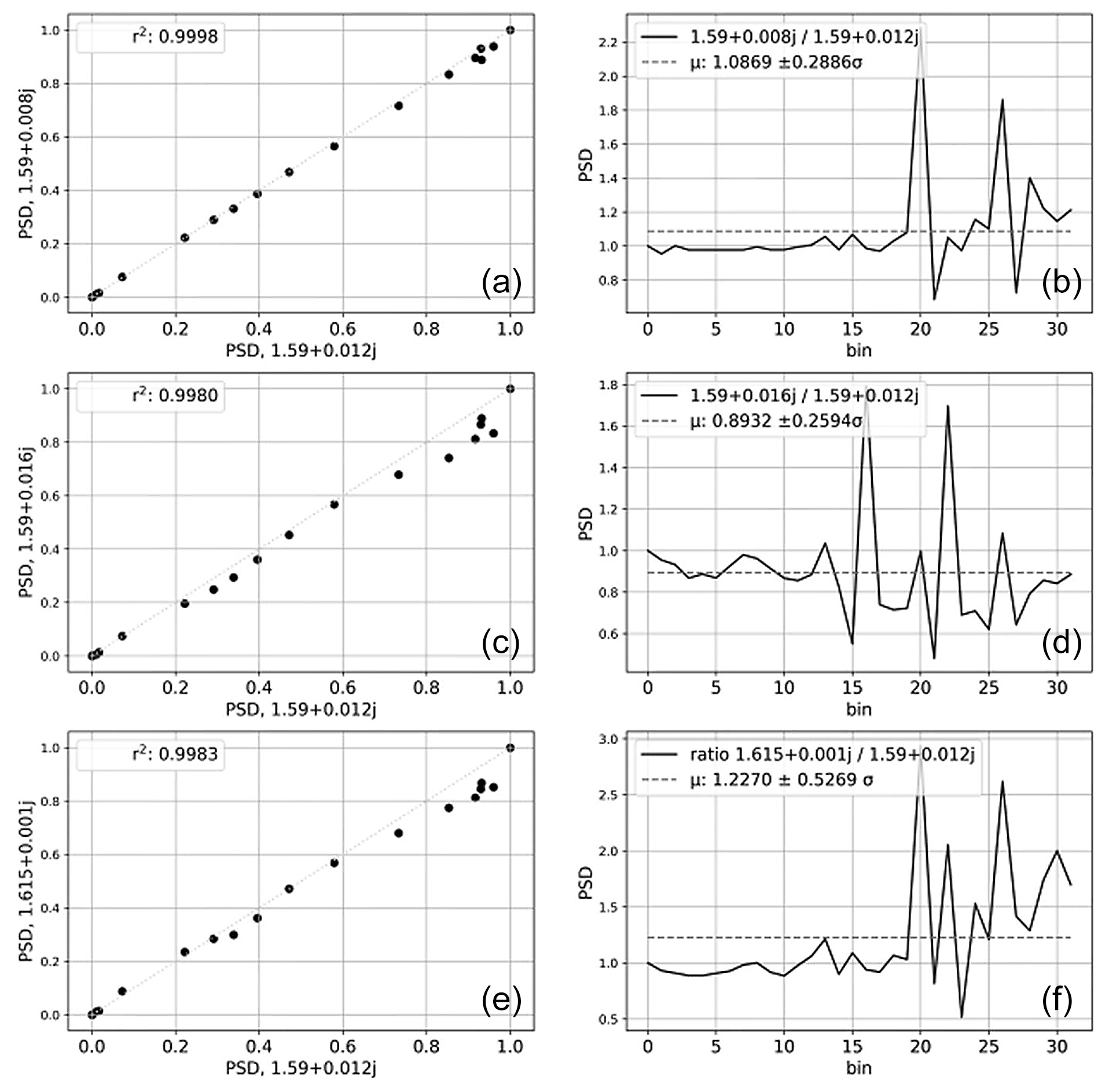
Figure B3Regression analysis (a, c, e) and corresponding ratios (b, d, f) of flight M270 run 0 normalised particle size distribution (PSD) derived using IOR = 1.59 + 0.012j (IORDER) against PSD derived from IOR = 1.59 + 0.008j (IORMAX, a, b), IOR = 1.59 + 0.016j (IORMIN, c, d) and IOR = 1.615 + 0.001j (IORPSL, e, f).
Regression analysis (Fig. B3, left column) of normalised PSDs corrected to IORMIN (top), IORMAX (middle) and IORPSL (bottom) against IORDER shows good agreement, with an r2 of 0.9998, 0.9980 and 0.9983, respectively. Mean differences between IORMIN : IORDER, IORMAX : IORDER and IORPSL : IORDER (Fig. B3, right column) are 9 %, 10 % and 23 %, respectively. The comparatively large uncertainty between corrected and uncorrected size distributions underlines the importance of accounting for IOR corrections when making ambient aerosol measurements. Mean differences in all comparisons are largest where Dp ⪆ 0.4 µm (PSD bin 15). Particle sizes in this region are comparable to the wavelength of light of the POPS (405 nm), which are the most efficient at scattering short-wave radiation, and sizes larger than this can be influenced by Mie resonances (Liu and Daum, 2000).
Flight M270 was chosen based on it showing significant variability compared to other Clean Air flights; uncertainty in using a flight-mean IOR for less varying flights is expected to be less. For example, flight M302, a typical London survey on 22 July 2021, performed numerous runs at altitudes ≈ 0.5 km and yields a difference of < 2 % between distributions corrected by IORMIN and IORMAX.
In summary, we conclude that use of a flight-mean IOR approach in correcting size distribution data introduces modest uncertainty of < 10 % compared to applying a variable IOR approach.
As discussed in Sect. 2.8, mass concentration (PM2.5) is derived from particle volume using the mean of a range of UK field experiments, which are detailed in Table C1.
Table C1Average chemical composition and density (g cm−3) of UK PM2.5, where H2004_ub and H2004_ubhp are Harrison et al. (2004) urban background and urban background high pollution, respectively. High-pollution percentages represent findings by Harrison et al. (2004), who reported an approximate doubling of concentrations of elemental carbon, organic compounds, sodium nitrate, ammonium sulfate, calcium sulfate and iron-rich dusts on high-pollution days and an increase of more than 5-fold in the ammonium nitrate concentration. AG2012_ub is Air Quality Expert Group (2012) urban background; H2008_ab is Haywood (2008). Airborne measurements are derived from the Facility for Airborne Atmospheric Measurements Bae146 over three flights (shown as reference ranges only). H2008_abmed, H2008_abmo and H2008_ abmi denote median, maximum organics and maximum inorganics, respectively, for H2008_ab percentage ranges. Index of refraction and density: the numbers in square brackets refer to the reference for the associated value, which are as follows: [1] Morgan et al. (2010), [2] Haywood (2008), [3] Hinds (1999), [4] Lafon et al. (2006), [5] Bond and Bergstrom (2006), [6] Hoon Jung et al. (2016), [7] CAMEO chemicals (NOAA, 2021), [8] National Center for Biotechnology Information (2023). An assumed density of 1 g cm−3 is used for “Other (incl. bound water)”.
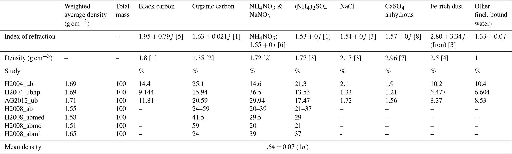
Figure D1 shows model and observed NO2 concentration throughout the second and third stacked box patterns performed around Birmingham during M296. Here, we see the intermediate stages of the plume as it begins to transition from the western quadrant of the city to the south-east with increasing altitude and time. As with runs 1 and 4, a comparison of NO2 aloft with average surface level observations shows similar concentrations, and the plume is not captured by the model.
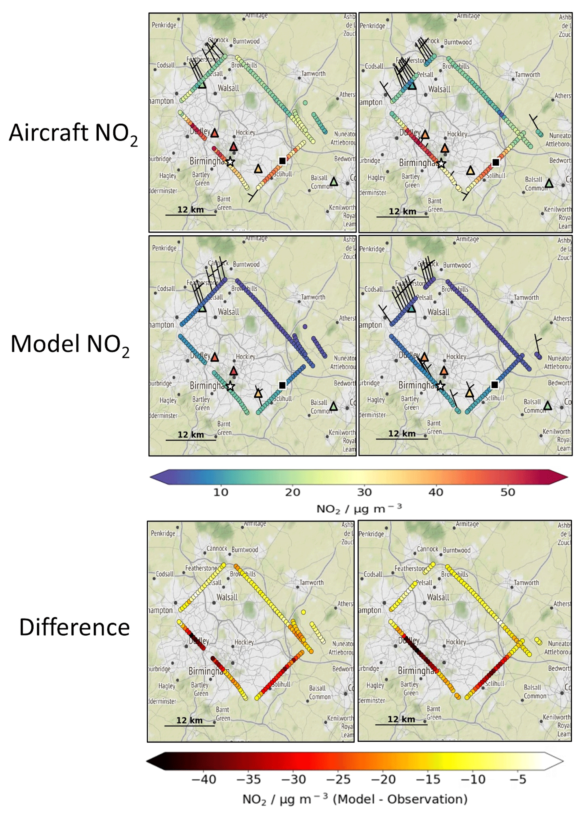
Figure D1Aircraft flight tracks coloured by NO2 concentration (µg m−3) for the second (left, 11:43:00 to 12:10:00 UTC) and third (right, 12:10:00 to 12:33 UTC) circuit, at altitudes of 511 and 573 m, respectively, around Birmingham during flight M296 on 1 July 2021. The top row shows the aircraft data. The middle row shows the model data. The bottom row shows the difference between the model and observations. Observation data are from straight and wing level transects, and all data are averaged over 10 s intervals. Wind barbs are only shown where the observed wind components exceed the measurement uncertainty. Data in triangles are the hourly surface level AURN NO2 concentration for the circuit. Stars and squares show the location of the Birmingham supersite and airport, respectively. Map tiles by Stamen Design, under CC BY 3.0. Data by OpenStreetMap, under ODbL.
Data are openly available from the CEDA (MOASA Clean Air Project: airborne atmospheric measurements collection) repository (https://doi.org/10.5285/0aa1ec0cf18e4065bdae8ae39260fe7d, Met Office and Mynard, 2023).
JK, AW, DT and JB instrumented the MOASA. JK, AW, KW, JML, NN, ERS and AM developed and planned flight sorties, and JK, AW and KW carried them out. AM designed, developed, and applied the post-flight quality assurance and processing software, where the NO2 module, including development of the pressure-dependent baseline correction, is adapted from original code by JML. ERS provided the AQUM model data, and ERS and BD assisted the observation–model comparison. AM, JML and SJA conceptualised the analysis (Sect. 4), and AM performed the formal analysis. MH devised and wrote the SPF Clean Air research programme, of which the MOASA flights are an integral part, acquired the financial support for the project and contributed to the original concept of a prolonged observation campaign. NN led the conceptualisation of MOASA involvement in the IOPs. AM prepared the manuscript with contributions from JML, ERS, JK, KW, SJA and MH.
The contact author has declared that none of the authors has any competing interests.
Publisher’s note: Copernicus Publications remains neutral with regard to jurisdictional claims in published maps and institutional affiliations.
The authors acknowledge and thank Alto Aerospace for efforts in delivering flight operations; the Met Office Guidance Unit, who have supported flight planning throughout; Kate Szpek and Nick Davies, whose nephelometer and TAP (respectively) processing software were adapted for this work; and Debbie O'Sullivan for creating Fig. 1.
All map tiles have been created with Stamen Design (https://stamen.com/, last access: 13 September 2023), under CC BY 3.0 (https://creativecommons.org/licenses/by/3.0/, last access: 13 September 2023). Data are from OpenStreetMap (https://openstreetmap.org, last access: 13 September 2023), under the Open Database License (https://www.openstreetmap.org/copyright, last access: 13 September 2023).
The MOASA Clean Air project is supported by the Clean Air programme, which is jointly delivered by the Natural Environment Research Council (NERC) and the Met Office, with the Economic and Social Research Council (ESRC), Engineering and Physical Sciences Research Council (EPSRC), Innovate UK, Medical Research Council (MRC), National Physical Laboratory (NPL), Science and Technology Facilities Research Council (STFC), Department for Environment, Food and Rural Affairs (Defra), Department for Health and Social Care (DHSC), Department for Transport (DfT), the Scottish Government, and the Welsh Government.
This paper was edited by Markus Rapp and reviewed by two anonymous referees.
Air Quality Expert Group: Fine Particulate Matter (PM2.5) in the United Kingdom, Department for Environment Food and Rural Affairs (DEFRA), https://uk-air.defra.gov.uk/assets/documents/reports/cat11/1212141150_AQEG_Fine_Particulate_Matter_in_the_UK.pdf (last access: 15 February 2021), 2012.
Air Quality Expert Group: Estimation of changes in air pollution emissions, concentrations and exposure during the COVID-19 outbreak in the UK, UK Air Inf. Resour., 1–57, https://uk-air.defra.gov.uk/assets/documents/reports/cat09/2007010844_Estimation_of_Changes_in_Air_Pollution_During_COVID-19_outbreak_in_the_UK.pdf (last access: 6 January 2021), 2020.
Bates, K. H. and Jacob, D. J.: An Expanded Definition of the Odd Oxygen Family for Tropospheric Ozone Budgets: Implications for Ozone Lifetime and Stratospheric In fl uence Geophysical Research Letters, Geophys. Res. Lett., 47, e2019GL084486, https://doi.org/10.1029/2019GL084486, 2019.
Beecken, J., Mellqvist, J., Salo, K., Ekholm, J., and Jalkanen, J.-P.: Airborne emission measurements of SO2, NOx and particles from individual ships using a sniffer technique, Atmos. Meas. Tech., 7, 1957–1968, https://doi.org/10.5194/amt-7-1957-2014, 2014.
Bond, T. C. and Bergstrom, R. W.: Light absorption by carbonaceous particles: An investigative review, Aerosol Sci. Tech., 40, 27–67, https://doi.org/10.1080/02786820500421521, 2006.
Bond, T. C., Anderson, T. L., and Campbell, D.: Calibration and Intercomparison of Filter-Based Measurements of Visible Light Absorption by Aerosols, Aerosol Sci. Tech., 30, 582–600, https://doi.org/10.1080/027868299304435, 1999.
Brechtel Manufacturing Inc: Model 1200 Isokinetic Aerosol Inlet System Manual ver. 8.0, manual, 2011.
Crilley, L. R., Singh, A., Kramer, L. J., Shaw, M. D., Alam, M. S., Apte, J. S., Bloss, W. J., Hildebrandt Ruiz, L., Fu, P., Fu, W., Gani, S., Gatari, M., Ilyinskaya, E., Lewis, A. C., Ng'ang'a, D., Sun, Y., Whitty, R. C. W., Yue, S., Young, S., and Pope, F. D.: Effect of aerosol composition on the performance of low-cost optical particle counter correction factors, Atmos. Meas. Tech., 13, 1181–1193, https://doi.org/10.5194/amt-13-1181-2020, 2020.
Dassios, K. G. and Pandis, S. N.: The mass accommodation coefficient of ammonium nitrate aerosol, Atmos. Environ., 33, 2993–3003, https://doi.org/10.1016/S1352-2310(99)00079-5, 1999.
Davies, N. W., Fox, C., Szpek, K., Cotterell, M. I., Taylor, J. W., Allan, J. D., Williams, P. I., Trembath, J., Haywood, J. M., and Langridge, J. M.: Evaluating biases in filter-based aerosol absorption measurements using photoacoustic spectroscopy, Atmos. Meas. Tech., 12, 3417–3434, https://doi.org/10.5194/amt-12-3417-2019, 2019.
DEFRA: Clean air strategy 2019, DEFRA, https://www.gov.uk/government/publications/clean-air-strategy-2019 (last access: 12 June 2020), 2019.
Denby, B., Cassiani, M., De Smet, P., De Leeuw, F., and Horálek, J.: Sub-grid variability and its impact on European wide air quality exposure assessment, Atmos. Environ., 45, 4220–4229, https://doi.org/10.1016/j.atmosenv.2011.05.007, 2011.
Dewline: DewLine™, Dewline, https://twobtech.com/dewline.html, last access: 15 May 2020.
Ecotech: Aurora3000 Integrating Nephelometer with backscatter, user manual v1.3, Ecotech, 2009.
El-Harbawi, M.: Air quality modelling, simulation, and computational methods: a review, Environ. Rev., 21, 149–179, https://doi.org/10.1139/er-2012-0056, 2013.
Environment Agency: Automatic Urban and Rural Network (AURN) LSO Manual, Version 1.2, Environment Agency, https://uk-air.defra.gov.uk/assets/documents/reports/empire/lsoman/lsoman.html (last access: 13 September 2023), 2022.
Fleming, R. J.: The use of commercial aircraft as platforms for environmental measurements, B. Amer. Meteorol. Soc., 77, 2229–2242, 1996.
Frie, A. L. and Bahreini, R.: Refractive index confidence explorer (RICE): A tool for propagating uncertainties through complex refractive index retrievals from aerosol particles, Aerosol Sci. Tech., 55, 703–717, https://doi.org/10.1080/02786826.2021.1895428, 2021.
Fuchs, N. A. and Sutugin, A. G.: High-dispersed aerosols, in: International Reviews in Aerosol Physics and Chemistry, Topics in Current Aerosol Research, edited by: Hidy, G. M. and Brock, J. R., Pergamon, https://doi.org/10.1016/B978-0-08-016674-2.50006-6, 1971.
Gao, R. S., Telg, H., McLaughlin, R. J., Ciciora, S. J., Watts, L. A., Richardson, M. S., Schwarz, J. P., Perring, A. E., Thornberry, T. D., Rollins, A. W., Markovic, M. Z., Bates, T. S., Johnson, J. E., and Fahey, D. W.: A light-weight, high-sensitivity particle spectrometer for PM2.5 aerosol measurements, Aerosol Sci. Tech., 50, 88–99, https://doi.org/10.1080/02786826.2015.1131809, 2016.
Grange, S. K., Lee, J. D., Drysdale, W. S., Lewis, A. C., Hueglin, C., Emmenegger, L., and Carslaw, D. C.: COVID-19 lockdowns highlight a risk of increasing ozone pollution in European urban areas, Atmos. Chem. Phys., 21, 4169–4185, https://doi.org/10.5194/acp-21-4169-2021, 2021.
Hagan, D. H. and Kroll, J. H.: Assessing the accuracy of low-cost optical particle sensors using a physics-based approach, Atmos. Meas. Tech., 13, 6343–6355, https://doi.org/10.5194/amt-13-6343-2020, 2020.
Harrison, R. M., Jones, A. M., and Lawrence, R. G.: Major component composition of PM10 and PM2.5 from roadside and urban background sites, Atmos. Environ., 38, 4531–4538, https://doi.org/10.1016/j.atmosenv.2004.05.022, 2004.
Haywood, J.: Prediction of visibility and aerosol within the operational Met Office Unified Model.II: Validation of model performance using observational data, Q. J. Roy. Meteor. Soc., 134, 1817–1832, https://doi.org/10.1002/qj.275, 2008.
Hinds, W. C.: Aerosol technology: properties, behavior, and measurement of airborne particles, John Wiley & Sons, ISBN 978-0-471-19410-1, 1999.
Hoon Jung, C., Jung Shin, H., Yi Lee, J., Pyo Kim, Y., Pitari, G., and Curci, G.: Sensitivity and Contribution of Organic Aerosols to Aerosol Optical Properties Based on Their Refractive Index and Hygroscopicity, Atmosphere, 7, 65, https://doi.org/10.3390/atmos7050065, 2016.
Kebabian, P. L., Herndon, S. C., and Freedman, A.: Detection of nitrogen dioxide by cavity attenuated phase shift spectroscopy, Anal. Chem., 77, 724–728, https://doi.org/10.1021/ac048715y, 2005.
Lafon, S., Sokolik, I. N., Rajot, J. L., Caquincau, S., and Gaudichet, A.: Characterization of iron oxides in mineral dust aerosols: Implications for light absorption, J. Geophys. Res.-Atmos., 111, 1–19, https://doi.org/10.1029/2005JD007016, 2006.
Langridge, J. M., Ball, S. M., Shillings, A. J. L., and Jones, R. L.: A broadband absorption spectrometer using light emitting diodes for ultrasensitive, in situ trace gas detection, Rev. Sci. Instrum., 79, 121310, https://doi.org/10.1063/1.3046282, 2008.
Langridge, J. M., Lack, D., Brock, C. A., Bahreini, R., Middlebrook, A. M., Neuman, J. A., Nowak, J. B., Perring, A. E., Schwarz, J. P., Spackman, J. R., Holloway, J. S., Pollack, I. B., Ryerson, T. B., Roberts, J. M., Warneke, C., De Gouw, J. A., Trainer, M. K., and Murphy, D. M.: Evolution of aerosol properties impacting visibility and direct climate forcing in an ammonia-rich urban environment, J. Geophys. Res.-Atmos., 117, 1–17, https://doi.org/10.1029/2011JD017116, 2012.
Liu, X., Chance, K., Sioris, C. E., Spurr, R. J. D., Kurosu, T. P., Martin, R. V., and Newchurch, M. J.: Ozone profile and tropospheric ozone retrievals from the Global Ozone Monitoring Experiment: Algorithm description and validation, J. Geophys. Res.-Atmos., 110, 1–19, https://doi.org/10.1029/2005JD006240, 2005.
Liu, Y. and Daum, P. H.: The effect of refractive index on size distributions and light scattering coefficients derived from optical particle counters, J. Aerosol Sci., 31, 945–957, https://doi.org/10.1016/S0021-8502(99)00573-X, 2000.
Lock, A. P., Martin, G. M., Bush, M. R., Brown, A. R., and Smith, R. N. B.: A new boundary layer mixing scheme part I: Tests in climate and mesoscale models, Mon. Weather Rev., 128, 3200–3217, https://doi.org/10.1175/1520-0493(2000)128<3200:ANBLMS>2.0.CO;2, 2000.
Manisalidis, I., Stavropoulou, E., Stavropoulos, A., and Bezirtzoglou, E.: Environmental and Health Impacts of Air Pollution: A Review, Front. Publ. Heal., 8, 1–13, https://doi.org/10.3389/fpubh.2020.00014, 2020.
McMeeking, G. R., Morgan, W. T., Flynn, M., Highwood, E. J., Turnbull, K., Haywood, J., and Coe, H.: Black carbon aerosol mixing state, organic aerosols and aerosol optical properties over the United Kingdom, Atmos. Chem. Phys., 11, 9037–9052, https://doi.org/10.5194/acp-11-9037-2011, 2011.
McMeeking, G. R., Bart, M., Chazette, P., Haywood, J. M., Hopkins, J. R., McQuaid, J. B., Morgan, W. T., Raut, J.-C., Ryder, C. L., Savage, N., Turnbull, K., and Coe, H.: Airborne measurements of trace gases and aerosols over the London metropolitan region, Atmos. Chem. Phys., 12, 5163–5187, https://doi.org/10.5194/acp-12-5163-2012, 2012.
Met Office and Mynard, A.: MOASA Clean Air Project: airborne atmospheric measurements collection, NERC EDS Centre for Environmental Data Analysis [data set], https://doi.org/10.5285/0aa1ec0cf18e4065bdae8ae39260fe7d, 2023.
Molina, M. J. and Molina, L. T.: Megacities and atmospheric pollution, J. Air Waste Manag. Assoc., 54, 644–680, https://doi.org/10.1080/10473289.2004.10470936, 2004.
Morgan, W. T., Allan, J. D., Bower, K. N., Esselborn, M., Harris, B., Henzing, J. S., Highwood, E. J., Kiendler-Scharr, A., McMeeking, G. R., Mensah, A. A., Northway, M. J., Osborne, S., Williams, P. I., Krejci, R., and Coe, H.: Enhancement of the aerosol direct radiative effect by semi-volatile aerosol components: airborne measurements in North-Western Europe, Atmos. Chem. Phys., 10, 8151–8171, https://doi.org/10.5194/acp-10-8151-2010, 2010.
Müller, T., Laborde, M., Kassell, G., and Wiedensohler, A.: Design and performance of a three-wavelength LED-based total scatter and backscatter integrating nephelometer, Atmos. Meas. Tech., 4, 1291–1303, https://doi.org/10.5194/amt-4-1291-2011, 2011.
Müller, T., Virkkula, A., and Ogren, J. A.: Constrained two-stream algorithm for calculating aerosol light absorption coefficient from the Particle Soot Absorption Photometer, Atmos. Meas. Tech., 7, 4049–4070, https://doi.org/10.5194/amt-7-4049-2014, 2014.
National Center for Biotechnology Information: PubChem Annotation Record for CALCIUM SULFATE, Hazardous Substances Data Bank (HSDB), https://pubchem.ncbi.nlm.nih.gov/compound/24497 (last access: 15 September 2023), 2023.
National Meteorological Library: Daily weather summary, September 2020, National Meteorological Library and Archive, https://digital.nmla.metoffice.gov.uk/IO_00cfff7c-7099-4583-ac85-a9adca963bb5/ (last access: 21 October 2021), 2020.
Neal, L. S., Agnew, P., Moseley, S., Ordóñez, C., Savage, N. H., and Tilbee, M.: Application of a statistical post-processing technique to a gridded, operational, air quality forecast, Atmos. Environ., 98, 385–393, https://doi.org/10.1016/j.atmosenv.2014.09.004, 2014.
Neal, L. S., Dalvi, M., Folberth, G., McInnes, R. N., Agnew, P., O'Connor, F. M., Savage, N. H., and Tilbee, M.: A description and evaluation of an air quality model nested within global and regional composition-climate models using MetUM, Geosci. Model Dev., 10, 3941–3962, https://doi.org/10.5194/gmd-10-3941-2017, 2017.
NOAA: CAMEO Chemicals, CAMEO Chem. version 2.7.1 rev 3, NOAA, https://cameochemicals.noaa.gov/chemical/25006, last access: 23 November 2021.
Nowak, J. B., Neuman, J. A., Bahreini, R., Brock, C. A., Middlebrook, A. M., Wollny, A. G., Holloway, J. S., Peischl, J., Ryerson, T. B., and Fehsenfeld, F. C.: Airborne observations of ammonia and ammonium nitrate formation over Houston, Texas, J. Geophys. Res.-Atmos., 115, 1–12, https://doi.org/10.1029/2010JD014195, 2010.
Ogren, J. A., Wendell, J., Andrews, E., and Sheridan, P. J.: Continuous light absorption photometer for long-term studies, Atmos. Meas. Tech., 10, 4805–4818, https://doi.org/10.5194/amt-10-4805-2017, 2017.
OSCA: http://www.ukcleanair.org (last access: 1 December 2021), 2020.
Peers, F., Francis, P., Fox, C., Abel, S. J., Szpek, K., Cotterell, M. I., Davies, N. W., Langridge, J. M., Meyer, K. G., Platnick, S. E., and Haywood, J. M.: Observation of absorbing aerosols above clouds over the south-east Atlantic Ocean from the geostationary satellite SEVIRI – Part 1: Method description and sensitivity, Atmos. Chem. Phys., 19, 9595–9611, https://doi.org/10.5194/acp-19-9595-2019, 2019.
Perim de Faria, J., Bundke, U., Freedman, A., Onasch, T. B., and Petzold, A.: Laboratory validation of a compact single-scattering albedo (SSA) monitor, Atmos. Meas. Tech., 14, 1635–1653, https://doi.org/10.5194/amt-14-1635-2021, 2021.
Petzold, A., Thouret, V., Gerbig, C., Zahn, A., Brenninkmeijer, C. A. M., Gallagher, M., Hermann, M., Pontaud, M., Ziereis, H., Boulanger, D., Marshall, J., NéDélec, P., Smit, H. G. J., Friess, U., Flaud, J. M., Wahner, A., Cammas, J. P., Volz-Thomas, A., Thomas, K., Rohs, S., Bundke, U., Neis, P., Berkes, F., Houben, N., Berg, M., Tappertzhofen, M., Blomel, T., Pätz, W., Filges, A., Boschetti, F., Verma, S., Baum, S., Athier, G., Cousin, J. M., Sauvage, B., Blot, R., Clark, H., Gaudel, A., Gressent, A., Auby, A., Fontaine, A., Gautron, B., Bennouna, Y., Petetin, H., Karcher, F., Abonnel, C., Dandin, P., Beswick, K., Wang, K. Y., Rauthe-Schöch, A., Baker, A. K., Riede, H., Gromov, S., Zimmermann, P., Thorenz, U., Scharffe, D., Koeppel, C., Slemr, F., Schuck, T. J., Umezawa, T., Ditas, J., Cheng, Y., Schneider, J., Williams, J., Neumaier, M., Christner, E., Fischbeck, G., Safadi, L., Petrelli, A., Gehrlein, T., Heger, S., Dyroff, C., Weber, S., Assmann, D., Rubach, F., Weigelt, A., Stratmann, G., Stock, P., Penth, L., Walter, D., Heue, K. P., Allouche, Y., Marizy, C., Hermira, J., Bringtown, S., Saueressig, G., Seidel, N., Huf, M., Waibel, A., Franke, H., Klaus, C., Stosius, R., Baumgardner, D., Braathen, G., Paulin, M., and Garnett, N.: Global-scale atmosphere monitoring by in-service aircraft – current achievements and future prospects of the European Research Infrastructure IAGOS, Tellus B, 6, 1–24, https://doi.org/10.3402/tellusb.v67.28452, 2015.
Qian, Y., Gustafson Jr., W. I., and Fast, J. D.: An investigation of the sub-grid variability of trace gases and aerosols for global climate modeling, Atmos. Chem. Phys., 10, 6917–6946, https://doi.org/10.5194/acp-10-6917-2010, 2010.
Rosenberg, P. D., Dean, A. R., Williams, P. I., Dorsey, J. R., Minikin, A., Pickering, M. A., and Petzold, A.: Particle sizing calibration with refractive index correction for light scattering optical particle counters and impacts upon PCASP and CDP data collected during the Fennec campaign, Atmos. Meas. Tech., 5, 1147–1163, https://doi.org/10.5194/amt-5-1147-2012, 2012.
Savage, N. H., Agnew, P., Davis, L. S., Ordóñez, C., Thorpe, R., Johnson, C. E., O'Connor, F. M., and Dalvi, M.: Air quality modelling using the Met Office Unified Model (AQUM OS24-26): model description and initial evaluation, Geosci. Model Dev., 6, 353–372, https://doi.org/10.5194/gmd-6-353-2013, 2013.
Solazzo, E., Bianconi, R., Pirovano, G., Moran, M. D., Vautard, R., Hogrefe, C., Appel, K. W., Matthias, V., Grossi, P., Bessagnet, B., Brandt, J., Chemel, C., Christensen, J. H., Forkel, R., Francis, X. V., Hansen, A. B., McKeen, S., Nopmongcol, U., Prank, M., Sartelet, K. N., Segers, A., Silver, J. D., Yarwood, G., Werhahn, J., Zhang, J., Rao, S. T., and Galmarini, S.: Evaluating the capability of regional-scale air quality models to capture the vertical distribution of pollutants, Geosci. Model Dev., 6, 791–818, https://doi.org/10.5194/gmd-6-791-2013, 2013.
Tang, W., Edwards, D. P., Emmons, L. K., Worden, H. M., Judd, L. M., Lamsal, L. N., Al-Saadi, J. A., Janz, S. J., Crawford, J. H., Deeter, M. N., Pfister, G., Buchholz, R. R., Gaubert, B., and Nowlan, C. R.: Assessing sub-grid variability within satellite pixels over urban regions using airborne mapping spectrometer measurements, Atmos. Meas. Tech., 14, 4639–4655, https://doi.org/10.5194/amt-14-4639-2021, 2021.
Thermo Scientific: Thermo Scientific Model 43 i Sulfur Dioxide Analyzer – pulsed fluorescence gas analyzer, Thermo Fisher Scientific Inc., https://assets.thermofisher.com/TFS-Assets%2FLSG%2FSpecification-Sheets%2FEPM-43i-Datasheet.pdf, last access: 24 May 2023.
UKRI: Integrated Research Observation System for Clean Air (OSCA), UK Research and Innovation, https://gtr.ukri.org/projects?ref=NE%2FT001984%2F1 (last access: 2 November 2021), 2021.
Veefkind, J. P., Aben, I., McMullan, K., Förster, H., de Vries, J., Otter, G., Claas, J., Eskes, H. J., de Haan, J. F., Kleipool, Q., van Weele, M., Hasekamp, O., Hoogeveen, R., Landgraf, J., Snel, R., Tol, P., Ingmann, P., Voors, R., Kruizinga, B., Vink, R., Visser, H., and Levelt, P. F.: TROPOMI on the ESA Sentinel-5 Precursor: A GMES mission for global observations of the atmospheric composition for climate, air quality and ozone layer applications, Remote Sens. Environ., 120, 70–83, https://doi.org/10.1016/j.rse.2011.09.027, 2012.
Virkkula, A.: Calibration of the 3-wavelength particle soot absorption photometer (3λ PSAP), Aerosol Sci. Tech., 44, 706–712, https://doi.org/10.1080/02786826.2010.482110, 2010.
von der Weiden, S.-L., Drewnick, F., and Borrmann, S.: Particle Loss Calculator – a new software tool for the assessment of the performance of aerosol inlet systems, Atmos. Meas. Tech., 2, 479–494, https://doi.org/10.5194/amt-2-479-2009, 2009.
Williams, M. L., Beevers, S., Kitwiroon, N., Dajnak, D., Walton, H., Lott, M. C., Pye, S., Fecht, D., Toledano, M. B., and Holland, M.: Public health air pollution impacts of pathway options to meet the 2050 UK Climate Change Act target: a modelling study, Publ. Heal. Res., 6, 1–124, https://doi.org/10.3310/phr06070, 2018.
Wilson, K. L. and Birks, J. W.: Mechanism and elimination of a water vapor interference in the measurement of ozone by UV absorbance, Environ. Sci. Technol., 40, 6361–6367, https://doi.org/10.1021/es052590c, 2006.
World Health Organization: Evolution of WHO air quality guidelines: past, present and future, WHO Regional Office for Europe, Copenhagen, Denmark, ISBN 9789289052306, 2017.
Wyche, K. P., Nichols, M., Parfitt, H., Beckett, P., Gregg, D. J., Smallbone, K. L., and Monks, P. S.: Changes in ambient air quality and atmospheric composition and reactivity in the South East of the UK as a result of the COVID-19 lockdown, Sci. Total Environ., 755, 142526, https://doi.org/10.1016/j.scitotenv.2020.142526, 2021.
- Abstract
- Introduction
- Measurement capability
- Observation and data strategy
- Example case studies
- Summary and conclusions
- Appendix A: AQ box schematic
- Appendix B: Index of refraction
- Appendix C: PM2.5 composition and density
- Appendix D: M296 runs 2 and 3
- Data availability
- Author contributions
- Competing interests
- Disclaimer
- Acknowledgements
- Financial support
- Review statement
- References