Broadband radiative quantities for the EarthCARE mission: the ACM-COM and ACM-RT products

The EarthCARE satellite mission's objective is to retrieve profiles of aerosol and water cloud physical properties from measurements made by its cloud-profiling radar, backscattering lidar, and passive multi-spectral imager. These retrievals, together with other geophysical properties, are input into broadband (BB) radiative transfer (RT) models that predict radiances and fluxes commensurate with measurements made and inferred from EarthCARE's BB radiometer (BBR). The scientific goal is that modelled and “observed” BB top-of-atmosphere (TOA) fluxes differ, on average, by less than ±10 W m⁻². When sound synergistic retrievals from the ACM-CAP process (ACM: ATLID – backscattering lidar, CPR – cloud-profiling radar, and MSI – multi-spectral imager; CAP: clouds, aerosols, and precipitation) are available, they are acted on by the RT models. When they are not available, the RT models act on “composite” profiles of properties retrieved from measurements made by individual sensors. Compositing is performed in the ACM-COM (COM: composite) process.

The majority of this report describes the RT models – and their products – that make up EarthCARE's ACM-RT process. Profiles of BB shortwave (SW) and longwave (LW) fluxes and heating rates (HRs) are computed by 1D RT models for each ∼ 1 km nadir column of inferred properties. Three-dimensional RT models compute radiances for the BBR's three viewing directions, with the SW model also computing flux and HR profiles; the 3D LW model produces upwelling flux at just one level. All 3D RT products are averages over 5×21 km “assessment domains” that are constructed using MSI data. Some of ACM-RT's products are passed forward to the “radiative closure assessment” process that quantifies, for each assessment domain, the likelihood that EarthCARE's goal has been achieved. As EarthCARE represents the first mission to make “operational” use of 3D RT models, emphasis is placed on differences between 1D and 3D RT results. For upwelling SW flux at 20 km altitude, 1D and 3D values can be expected to differ by more than EarthCARE's scientific goal of ±10 W m⁻² at least 50 % of the time.

1 Introduction

The EarthCARE satellite mission's primary objective is to make avant-garde observations of Earth's atmosphere that can be used to help improve representations of clouds and aerosols in numerical models that predict weather, air quality, and climatic change (Illingworth et al., 2015). Detailed descriptions of observations made by EarthCARE's cloud-profiling radar (CPR), backscattering lidar (ATLID), passive multi-spectral imager (MSI), and broadband radiometer (BBR), as well as the L2 retrieval algorithms that operate on them, are discussed in several papers of this special issue (Eisinger et al., 2023). EarthCARE's scientific goal is to retrieve cloud and aerosol properties with enough accuracy that when operated on by broadband (BB) radiative transfer (RT) models, their estimated top-of-atmosphere (TOA) BB fluxes for domains covering ∼ 100 km² agree more often than not with their BBR-derived counterparts (Velázquez-Blázquez et al., 2023a) to within ±10 W m⁻² (ESA, 2001). This “radiative closure assessment”, which marks the end of the initial version of EarthCARE's formal “data production chain”, provides a continuous radiative closure assessment of L2 retrievals with invaluable information for both L2 algorithm developers and data users.

The primary purpose of this paper is to describe and demonstrate the BB RT models used for both radiative closure assessment and provision of BB flux and heating rate (HR) profiles. Application of BB RT models to L2 retrieval products, along with auxiliary data, such as profiles of state variables and surface optical properties, will provide estimates of a range of diagnostic radiative flux and HR profiles. Examples of these products are presented here for simulated conditions along ∼ 6200 km long sections of EarthCARE orbits, which are referred to as “frames” (Qu et al., 2022). These simulations underpin most experiments reported in this special issue.

Both 1D and 3D shortwave (SW) and longwave (LW) RT models are used. Both SW and LW 3D models produce TOA radiances; the SW model also produces flux and HR profiles for all-sky conditions for a subset of ∼ 100 km² assessment domains, while the LW model produces upwelling fluxes at a single level. The number of radiative closure assessment domains that can be processed per frame changes from frame to frame and will depend on computer resource availability during the mission as well as, to a lesser extent, cloud structure. Both SW and LW 1D models produce flux and HR profiles for each L2 column for all-sky, clear-sky (i.e., clouds removed), and pristine-sky (i.e., cloud and aerosol removed) conditions. This provides continuity with previous and ongoing missions such as CloudSat (Stephens et al., 2002) and CERES (Wielicki et al., 1996). All applications of RT models occur in the processor referred to as ACM-RT. As for other EarthCARE processors, the prefix indicates instrument(s) whose data provide input data, while the suffix represents an abbreviation of the current processor; in this case, ACM stands for ATLID, CPR, and MSI, and RT stands for radiative transfer.

The current plan is for RT models to be applied to cloud and aerosol profile retrievals from the ACM-CAP (CAP: clouds, aerosols, and precipitation) process's Cloud, Aerosol and Precipitation from mulTiple Instruments using a VAriational TEchnique (CAPTIVATE) algorithm (Mason et al., 2023). ACM-CAP's products, which are in the L2b class of products, are recognized formally as EarthCARE's “best estimates” for they represent the most complete synergistic use of observations made by the CPR, ATLID, and MSI. Should CAPTIVATE fail, the contingency plan is to use a composite back-up best estimate based on products arising from retrieval algorithms that operate on measurements from a single active sensor. These products are in the L2a class. As such, the secondary purpose of this paper is to describe how the composite cloud and aerosol profiles are generated within the ACM-COM (COM: composite) process.

The following section provides an overview of the ACM-COM and ACM-RT processes and how they link to other processes. This is followed by a description of how EarthCARE retrievals are prepared for use in RT models including the creation of L2a composite (back-up) cloud–aerosol profiles. In Sect. 4 the SW and LW RT models are described along with atmospheric and surface optical properties. RT model results are documented in Sect. 5, making use of the synthetic test frames. This includes showing the full extent of products from the 1D models and differences between SW and LW fluxes predicted by 1D and 3D RT models. Section 6 provides a summary.

2 Overview of EarthCARE's radiation products

Figure 1 encapsulates the main operations of ACM-COM and ACM-RT including its inputs and outputs. ACM-COM prepares profiles of cloud and aerosol properties produced by L2 retrieval processors, as summarized by Eisinger et al. (2023), for use by the BB RT models in ACM-RT. The main operations of these processors are addressed in the subsequent two sections. The remainder of this section provides an overview of the components in Fig. 1.

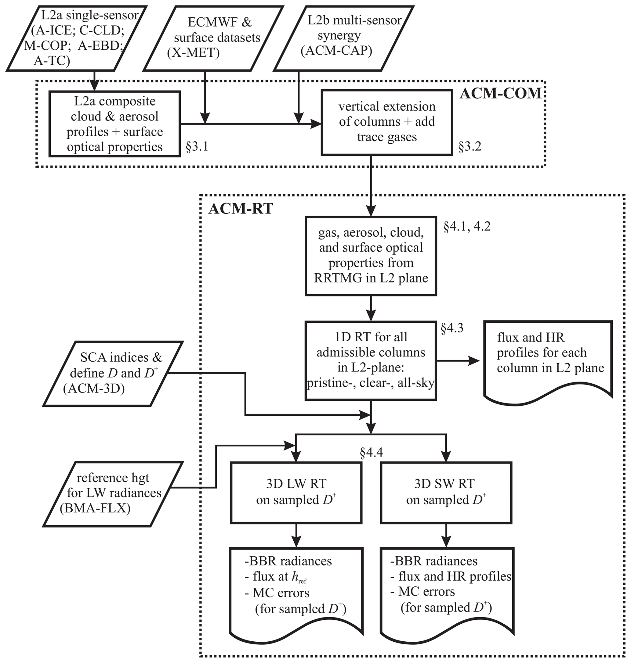
Figure 1 Flowchart summarizing the basic inputs to the ACM-COM and ACM-RT processes, their core operations, and their permanent output files. The operations are discussed in the sections listed next to them.

Arriving at ACM-COM are profiles of cloud and aerosol properties for each column in the mission's joint standard grid (JSG) (Eisinger et al., 2023), along the L2 plane, as retrieved by single-active-sensor L2a algorithms. ACM-COM also receives similar profiles produced by the synergistic L2b CAPTIVATE algorithm in ACM-CAP, which utilizes ATLID, CPR, and MSI measurements (Mason et al., 2023). While studies to date suggest that ACM-CAP products will likely be EarthCARE's default best estimates (Mason et al., 2023), this will not be known for sure until EarthCARE's post-launch “commissioning phase”. Should ACM-CAP fail and thus leave only (some) L2a retrievals usable by RT models, a contingency plan was developed in which L2a products are merged to form alternate best-estimate composite cloud–aerosol profiles. Compositing of L2a products is explained in Sect. 3.2.

Regardless of whether ACM-CAP or alternate L2a composite profiles are acted on by ACM-RT's RT models, they need to be readied for use there. Hence, the last steps of ACM-COM take profiles of meteorological variables and surface conditions, passed in from the auXiliary METeorology (X-MET) processor (Eisinger et al., 2023) and databases, respectively, and merge them with ACM-CAP or L2a composite products.

Following previous satellite missions (e.g., L'Ecuyer et al., 2008; Kato et al., 2013), ACM-RT computes SW and LW BB flux and HR profiles by applying 1D RT models to each admissible JSG profile along the L2 plane. EarthCARE makes a substantial step forward, however, with its operational use of 3D BB RT models for both SW and LW bands. For consistency, 1D and 3D models use, where possible, common descriptions of atmospheric and surface optical properties. Optical properties for pristine atmospheres, free of aerosol and clouds, come from the Rapid Radiative Transfer Model for General Circulation Models (RRTMG) (Iacono et al., 2008; Morcrette et al., 2008). RRTMG's SW and LW 1D two-stream models compute flux and HR profiles for each JSG column along the L2 plane. The default is to use all ACM-CAP profiles available in an EarthCARE frame. If no ACM-CAP profiles are available, or if there is an explicit request for radiative closure assessment to be performed on ACM-COM results, radiative transfer calculations are performed for the L2a composite profiles. These results are passed to ACMB-DF (B: BBR; DF: difference in fluxes) (Barker et al., 2023), where they are averaged over radiative closure assessment domains (D's) as dictated by the ACMB-3D (3D: three-dimensional) scene construction algorithm indices (Qu et al., 2023).

The 3D RT solvers are Monte Carlo solutions of the plane-parallel 3D RT equation. They use the same gaseous, aerosol, and cloud optical properties as the 1D models, but they use detailed scattering phase functions. The SW model produces profiles of fluxes and HRs and TOA BB radiances commensurate with the BBR's three telescopes. The LW model computes the same radiances along with an upwelling flux at a “reference height”, as defined in the BMA-FLX (FLX: fluxes) process (Velázquez-Blázquez et al., 2023a). All 3D RT computations are done for “radiation computation domains” (D⁺'s) that consist of D and buffer zones around them (see Fig. 2). Model estimates of radiances and fluxes and any available uncertainties are averaged over D and passed to the ACMB-DF processor (Barker et al., 2023) where they are compared to BBR radiances and their model-derived fluxes (Velázquez-Blázquez et al., 2023a, b).

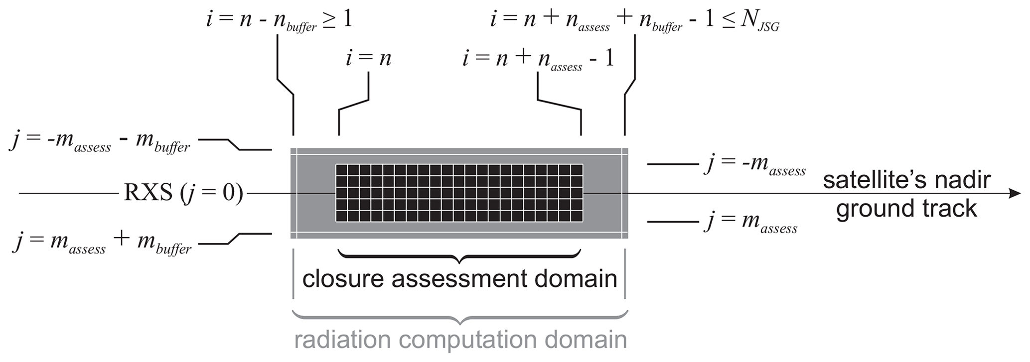
Figure 2 Schematic showing the radiative closure assessment domain D (black) and extended computation domain D⁺ (shaded), which is the union of D and its buffer zones. These domains are centred on the L2a/L2b retrieved cross-section (RXS). See Qu et al. (2022, 2023) for details.

3 ACM-COM: preparations for RT models and L2a composites

As described in the next subsection, ACM-COM readies, for use by RT models in ACM-RT, cloud and aerosol information from various L2 retrieval processes and meteorological information from X-MET. This is followed by an explanation of how ACM-CAP's alternate L2 composite profiles are produced.

3.1 Prepping L2 retrievals for RT models

The ACM-COM process begins by simply extracting, from X-MET files, information about atmospheric state, as needed by all BB RT models. This includes profiles of pressure, temperature, humidity, and ozone concentration. Regarding aerosols, their classification information is provided by the AC-TC (TC: target classification) processor (Irbah et al., 2023a) with extinction profiles at 0.355 µm obtained from the A-EBD (EBD: extinction backscatter depolarization) product (Donovan et al., 2023). Six types of aerosols are considered: dust, sea salt, continental pollution, smoke, dusty smoke, and dusty mix. Grid cells in AC-TC that are classed as cloudy, uncertain, missing, or noisy are considered to be aerosol-free.

Additionally, ACM-COM adds the following minor molecular species to X-MET profiles: CO₂, CH₄, N₂O, CFC-11, CFC-12, CFC-22, and CCL4. These profiles come from climatologies generated by Jean-Jacques Morcrette and Alessio Bozzo (Robin Hogan personal communication, 2013). Values are functions of month, pressure, and latitude.

3.2 Construction of “L2a composite” cloud and aerosol profiles

This subsection describes the algorithm that produces the alternative to ACM-CAP's synergistic L2b best estimates. It is based on compositing L2a cloud microphysical property retrievals from A-ICE (ICE: ice microphysical estimation) (Donovan et al., 2023a) and C-CLD (CLD: cloud) (Mroz et al., 2023) products.

The L2a composite's cloud properties depend on an indication of columnar cloudiness from the M-COP (COP: cloud optical properties) processor (Hünerbein et al., 2023). If a grid cell in a column has either A-ICE or C-CLD cloud water content greater than zero, the reported cloud properties enter directly into the L2a composite. If, however, both A-ICE and C-CLD report valid cloud properties with ice water content IWC >0, aggregated normalized uncertainties for IWC and crystal effective radius r_eff are computed, respectively, as

$$\begin{array}{}\text{(1)}& \begin{array}{rl}& {\mathit{\sigma }}_{\mathrm{A}-\mathrm{ICE}}=\sqrt{{\left({\displaystyle \frac{{\mathit{\sigma }}_{\mathrm{IWC}}^{\mathrm{A}-\mathrm{ICE}}}{{\text{IWC}}^{\mathrm{A}-\mathrm{ICE}}}}\right)}^{\mathrm{2}}+{\left({\displaystyle \frac{{\mathit{\sigma }}_{r_{\mathrm{eff}}}^{\mathrm{A}-\mathrm{ICE}}}{r_{\mathrm{eff}}^{\mathrm{A}-\mathrm{ICE}}}}\right)}^{\mathrm{2}}}\text{and}\\ & {\mathit{\sigma }}_{\mathrm{C}-\mathrm{CLD}}=\sqrt{{\left({\displaystyle \frac{{\mathit{\sigma }}_{\mathrm{IWC}}^{\mathrm{C}-\mathrm{CLD}}}{{\text{IWC}}^{\mathrm{C}-\mathrm{CLD}}}}\right)}^{\mathrm{2}}+{\left({\displaystyle \frac{{\mathit{\sigma }}_{r_{\mathrm{eff}}}^{\mathrm{C}-\mathrm{CLD}}}{r_{\mathrm{eff}}^{\mathrm{C}-\mathrm{CLD}}}}\right)}^{\mathrm{2}}},\end{array}\end{array}$$

where ${\mathit{\sigma }}_{\mathrm{IWC}}^{\mathrm{A}-\mathrm{ICE}}$, ${\mathit{\sigma }}_{\mathrm{IWC}}^{\mathrm{C}-\mathrm{CLD}}$, ${\mathit{\sigma }}_{r_{\mathrm{eff}}}^{\mathrm{A}-\mathrm{ICE}}$, and ${\mathit{\sigma }}_{r_{\mathrm{eff}}}^{\mathrm{C}-\mathrm{CLD}}$ are processor-specific 1σ uncertainties. Ice cloud properties for the product with $min\left({\mathit{\sigma }}_{\mathrm{A}-\mathrm{ICE}},{\mathit{\sigma }}_{\mathrm{C}-\mathrm{CLD}}\right)$ enter into the L2a composite. For grid cells designated to contain only liquid clouds, C-CLD properties are used. Hence, L2a composites resemble NASA's CloudSat–CALIPSO–CERES (C3M) product (Kato et al., 2010), though it is simpler in that active-sensor-derived water content is not constrained, as it is in ACM-CAP, by MSI passive radiances.

Figure 3 shows an example of this compositing process for a column from a simulated frame (Qu et al., 2022). Only ice clouds were present, so both A-ICE and C-CLD reported hydrometeors. Above ∼ 3.4 km ATLID's estimates have the least uncertainty, meaning that A-ICE values enter into the composite. At ∼ 3.3 km the CPR value is least uncertain, and so C-CLD's estimate is used. As ATLID failed to return useable signals at lower altitudes, CPR values fill the remainder of ACM-COM's profile.

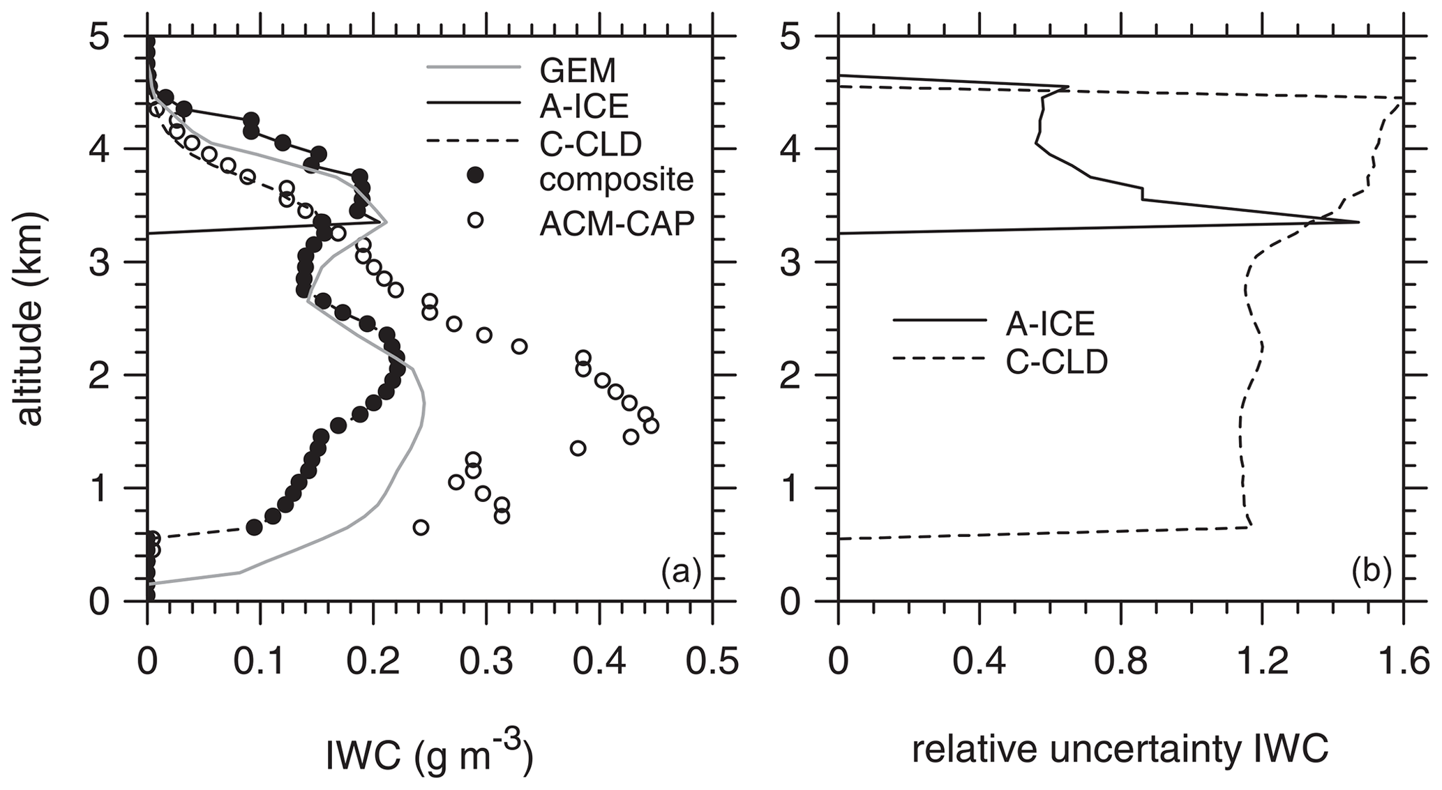
Figure 3 (a) Lines represent profiles of IWC directly from the test frame (simulated by GEM), as well as those retrieved by the L2a algorithms in processors A-ICE and C-CLD. Filled circles are layer values that ACM-COM's algorithm selected from A-ICE and C-CLD according to which one has the smallest aggregated relative uncertainty, defined by Eq. (1), as shown in panel (b). This profile, which has only ice clouds, is from the Halifax test frame at 63.67^∘ N, 54.64^∘ W.

In this example, the “reference values”, as simulated by the Global Environmental Multiscale (GEM) model (Qu et al., 2022), generally match ACM-COM's better than ACM-CAP's. This, however, does not mean that ACM-COM profiles will be used by the RT models. First, during the mission reference values are, of course, unknown, so a plot like Fig. 3 cannot be made or used. Second, if and when ACM-CAP profiles exist, they are used by default.

4 ACM-RT: broadband radiative transfer models

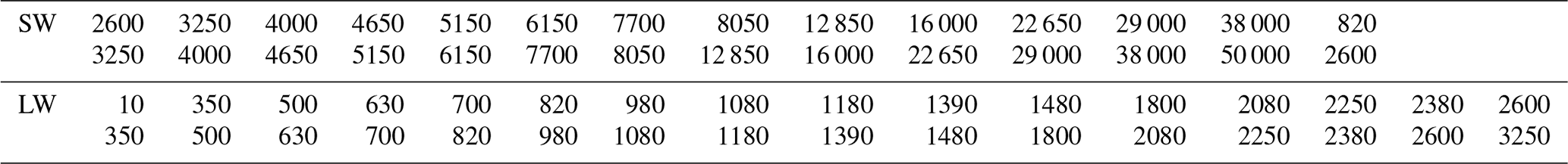
As mentioned above, EarthCARE's RT models are based on RRTMG (Iacono et al., 2003, 2008; Morcrette et al., 2008). Like its computationally taxing progenitor (Mlawer et al., 1997; Mlawer and Clough, 1998), RRTMG is built on the correlated k distribution (CKD) method (Goody et al., 1989; Lacis and Oinas, 1991). Broadband integrated flux and HR profiles are sums of calculations for quadrature points (112 for SW and 140 for LW) spread over spectral bands (14 for SW and 16 for LW; Table 1). RRTMG is used widely in large-scale models, and its verification has been documented elsewhere (e.g., Iacono et al., 2008; Oreopoulos et al., 2012). This section begins by describing atmospheric and surface optical properties and follows with descriptions of the 1D and 3D transport solvers.

Table 1 Wavenumber intervals used in SW and LW RRTMG models. Wavenumbers are in inverse centimetres (cm⁻¹).

4.1 Optical properties: atmospheric constituents

4.1.1 Gases

Molecular optical depths are computed by the CKD method in RRTMG_SW_v3.9 and RRTMG_LW_v4.85 for several wavenumber intervals (Table 1) and used by both 1D and 3D RT models. The SW CKD model accounts for absorption by H₂O, CO₂, O₃, CH₄, O₂, and N₂ plus Rayleigh scattering, while the LW CKD model accounts for absorption by H₂O, CO₂, O₃, N₂O, CH₄, O₂, N₂, CFC11, CFC12, CFC22, and CCl₄. A continuum model, CKD_v2.4, accounts for foreign broadening and self-broadening of lines for H₂O, CO₂, O₂, O₃, and Rayleigh scattering. Molecular absorption coefficients for RRTMG's k distributions were obtained from the line-by-line RT model (LBLRTM), which has been evaluated against surface and laboratory observations (Clough et al., 2005; Shephard et al., 2009; Alvarado et al., 2013). LBLRTM's spectroscopic line parameters are essentially equivalent to HITRAN 2000 and HITRAN 1996 (SW) databases. Algorithmic accuracy of LBLRTM is 0.5 % (Clough et al., 2005), with limiting errors generally attributed to line shape and spectroscopic input parameters.

For 1D SW RT, the Rayleigh scattering phase function is approximated as p_Ray(μ)=1, where μ=cos θ, and θ is scattering angle. For 3D SW RT, on the other hand,

$$\begin{array}{}\text{(2)}& p_{\mathrm{Ray}}\left(\mathit{\mu }\right)={\displaystyle \frac{\mathrm{3}}{\mathrm{4}}}\left(\mathrm{1}+{\mathit{\mu }}^{\mathrm{2}}\right),\end{array}$$

which is, as are all phase functions used here, normalized as

$$\begin{array}{}\text{(3)}& {\displaystyle \frac{\mathrm{1}}{\mathrm{2}}}\underset{-\mathrm{1}}{\overset{\mathrm{1}}{\int }}{p}_{\mathrm{Ray}}\left(\mathit{\mu }\right)\mathrm{d}\mathit{\mu }=\mathrm{1}.\end{array}$$

Relative to LBLRTM, clear-sky RRTMG_LW BB fluxes at all levels are accurate to within ±1.5 W m⁻² (±1 W m⁻² for direct beams and ±2 W m⁻² for diffuse beams), with HRs agreeing to within ±0.2 K d⁻¹ in the troposphere and ±0.4 K d⁻¹ in the stratosphere. Likewise, RRTMG_SW's accuracies, at μ₀≈0.7, are within ±3 W m⁻² at all levels, with HRs agreeing to within ±0.1 K d⁻¹ in the troposphere and ±0.35 K d⁻¹ in the stratosphere.

4.1.2 Aerosols

As with gases, 1D and 3D RT models share the same spectral optical properties for aerosols: extinction coefficient β_aero, single-scattering albedo ω_aero, and asymmetry parameter g_aero. Spectral β_aero, ω_aero, and g_aero are averaged over the wavelength λ intervals listed above and generated so as to be consistent with retrieval algorithms following Wandinger et al. (2023). Radiative properties for their basic aerosol types are then mixed externally, yielding radiative properties for aerosol mixture classifications used in AC-TC. Aerosol extinction is provided at 355 nm, and so for each aerosol mixture the ratio ${\mathit{\beta }}_{\mathrm{aero}}\left(\mathit{\lambda }\right)/{\mathit{\beta }}_{\mathrm{aero}}\left(\mathrm{0.355}\mathrm{\mu }\mathrm{m}\right)$ at each λ is computed and then averaged spectrally using the same weightings as for cloud radiative properties as described below.

Aerosol scattering phase functions, as needed by the 3D RT codes, are represented by the Henyey–Greenstein function (Henyey and Greenstein, 1941), which is given by

$$\begin{array}{}\text{(4)}& p_{\mathrm{HG}}\left(\mathit{\mu };g_{\mathrm{aero}}\right)={\displaystyle \frac{\mathrm{1}-g_{\mathrm{aero}}^{\mathrm{2}}}{{\left(\mathrm{1}+g_{\mathrm{aero}}^{\mathrm{2}}-\mathrm{2}{g}_{\mathrm{aero}}\mathit{\mu }\right)}^{\mathrm{3}/\mathrm{2}}}},\end{array}$$

satisfies

$$\begin{array}{}\text{(5)}& g_{\mathrm{aero}}={\displaystyle \frac{\mathrm{1}}{\mathrm{2}}}\underset{-\mathrm{1}}{\overset{\mathrm{1}}{\int }}{p}_{\mathrm{HG}}\left(\mathit{\mu };g_{\mathrm{aero}}\right)\mathit{\mu }\mathrm{d}\mathit{\mu },\end{array}$$

and is used directly in the models (i.e., no need for tabulation). Owing to the size and irregularity of aerosol particles and retrieval uncertainties, use of Eq. (4) is reasonable.

4.1.3 Liquid clouds

The standard version of RRTMG uses the Hu and Stamnes (1993) parameterizations of spectral β, ω₀, and g for liquid droplets. For EarthCARE, however, these have been replaced by more precise Lorenz–Mie calculations tabulated for ranges of droplet effective radii r_eff and effective variances v_eff, which are defined, respectively, as

$$\begin{array}{}\text{(6)}& r_{\mathrm{eff}}={\displaystyle \frac{{\int }_{\mathrm{0}}^{\mathrm{\infty }}n\left(r\right)r^{\mathrm{3}}\mathrm{d}r}{{\int }_{\mathrm{0}}^{\mathrm{\infty }}n\left(r\right)r^{\mathrm{2}}\mathrm{d}r}}={\displaystyle \frac{〈r^{\mathrm{3}}〉}{〈r^{\mathrm{2}}〉}}\end{array}$$

and

$$\begin{array}{}\text{(7)}& v_{\mathrm{eff}}={\displaystyle \frac{{\int }_{\mathrm{0}}^{\mathrm{\infty }}{\left(r-r_{\mathrm{eff}}\right)}^{\mathrm{2}}n\left(r\right)r^{\mathrm{2}}\mathrm{d}r}{r_{\mathrm{eff}}^{\mathrm{2}}{\int }_{\mathrm{0}}^{\mathrm{\infty }}n\left(r\right)r^{\mathrm{2}}\mathrm{d}r}}={\displaystyle \frac{〈r^{\mathrm{2}}〉〈r^{\mathrm{4}}〉}{{〈r^{\mathrm{3}}〉}^{\mathrm{2}}}}-\mathrm{1},\end{array}$$

where r is droplet radius. Droplet size distributions n(r) are assumed (Chýlek et al., 1992) to be

$$\begin{array}{}\text{(8)}& n\left(r\right)={\displaystyle \frac{N}{\mathrm{\Gamma }\left(\mathit{\nu }\right)}}({\displaystyle \frac{\mathit{\nu }}{〈r〉}}{)}^{\mathit{\nu }}{r}^{\mathit{\nu }-\mathrm{1}}\exp \left(-{\displaystyle \frac{r\mathit{\nu }}{〈r〉}}\right),\end{array}$$

where 〈r〉=νr_effv_eff and $\mathit{\nu }=\left(\mathrm{1}-\mathrm{2}{v}_{\mathrm{eff}}\right)/v_{\mathrm{eff}}$.

Lorenz–Mie computations (Wiscombe, 1980), using the refractive indices of Segelstein (1981), were performed for r between 0.01 and 120 µm in increments of 0.05 µm and for wavelengths λ between 0.25 and 100 µm in increments of 0.02 for $\mathrm{0.25}<\mathit{\lambda }<\mathrm{2}$ µm, 0.04 for $\mathrm{2}<\mathit{\lambda }<\mathrm{3}$ µm, 0.05 for $\mathrm{3}<\mathit{\lambda }<\mathrm{10}$ µm, 0.07 for $\mathrm{10}<\mathit{\lambda }<\mathrm{20}$ µm, and 0.1 for $\mathrm{20}<\mathit{\lambda }<\mathrm{100}$ µm. Phase functions and optical properties were integrated over RRTMG's spectral intervals for combinations of r_eff and v_eff: r_eff from 0.5–40 µm in increments of 0.5 µm and ν_eff from 0.02–0.4 in increments of 0.02 µm. Spectral weightings for SW bands are the mean of downwelling irradiances at the tropopause and surface as predicted by a line-by-line RT model (Iacono et al., 2008) for the tropical atmosphere at solar zenith angle θ₀=0^∘. For LW bands, weightings are the Planck function at 275 K. In the RT models, values of r_eff and ν_eff are rounded to the nearest value in the table, which usually results in errors for β, ω₀, and g of less than ±1 %.

As the 3D RT models are Monte Carlo solutions, they use normalized tabulated scattering phase functions p(μ) for droplets. Broadband, spectrally integrated p(μ) have 1800 equal-angle bins, and their cumulative sums, as functions of μ, were computed by

$$\begin{array}{}\text{(9)}& R\left({\mathit{\mu }}_{\mathrm{s}}\right)={\displaystyle \frac{\mathrm{1}}{\mathrm{2}}}\underset{{\mathit{\mu }}_{\mathrm{s}}}{\overset{\mathrm{1}}{\int }}p\left(\mathit{\mu }\right)\mathrm{d}\mathit{\mu },\end{array}$$

where μ_s is cosine of the scattering angle, with $R\left({\mathit{\mu }}_{\mathrm{s}}=\mathrm{1}\right)=\mathrm{0}$ (forescatter) and $R\left({\mathit{\mu }}_{\mathrm{s}}=-\mathrm{1}\right)=\mathrm{1}$ (backscatter). For efficiency, tables of μ_s were constructed for 1800 equally spaced values of R; when a scattering event occurs, a uniform pseudo-random number gets generated $R\in \left[\mathrm{0},\mathrm{1}\right]$, and linear interpolation sets μ_s, which is used to update a photon's direction cosines.

4.1.4 Ice clouds

Values of β, ω₀, g, and scattering phase functions for ice clouds are based on the theoretical functions of Yang et al. (2013) for 11 crystal habits: droxtals, prolate spheroids, oblate spheroids, solid columns, hollow columns, aggregates composed of 8 solid columns, hexagonal plates, small aggregates composed of 5 plates, large aggregates composed of 10 plates, solid bullet rosettes, and hollow bullet rosettes. The maximum dimension for each habit ranges from 2 to 10 000 µm for 189 discrete sizes. Three surface roughness conditions were considered for each ice habit: smooth, moderate, and severe. Each constituent has volume, projected area, effective size, extinction efficiency, ω₀, and g. Their scattering phase functions are tabulated at 498 unequal angles but were transformed into 1800 equal-angle bins for use in Eq. (9).

To make this dataset's size suitable for operational use, optical properties were averaged over λ and assumed distributions of habit, size, and roughness that were derived from CALIPSO observations (Baum et al., 2011). Resulting phase functions and optical properties are functions of effective diameter, which is defined as

$$\begin{array}{}\text{(10)}& d_{\mathrm{eff}}={\displaystyle \frac{\mathrm{3}}{\mathrm{2}}}{\displaystyle \frac{\sum _i\int V_i\left(D\right)n\left(D\right)f_i\left(D\right)\mathrm{d}D}{\sum _i\int A_i\left(D\right)n\left(D\right)f_i\left(D\right)\mathrm{d}D}},\end{array}$$

where V, A, and D are geometric volume, orientation-averaged projected area, and maximum dimension of ice particle, respectively; n(D) denotes crystal size distribution, and f_i indicates the percentage of each ice particle habit and roughness. Values of d_eff range from 10 to 120 µm in increments of 5 µm. Band-averaged optical properties were computed using the same weightings as in Eq. (10) while also weighting for spectral irradiance and then integrating over RRTMG's spectral intervals. The spectral weight for SW bands was the TOA spectrum, while for the LW it was the Planck function at 250 K (Bingqi Yi, personal communication, 2013).

4.1.5 Solid hydrometeors and rain

Solid hydrometeors are retrieved as though they were ice clouds, and their optical properties appear as such. In addition to liquid cloud properties, however, ACM-CAP reports layer rain rates R (mm h⁻¹). Raindrop size distributions are assumed to follow the gamma distribution of Ulbrich (1983). Spectrally integrated single-scattering properties are defined using the same spectral weights as discussed in Sect. 4.1.3 in conjunction with Mie scattering properties for droplet radii between 10 and 2000 µm; larger drops tend to break up (e.g., Cotton and Gokhale, 1967). Tables of optical properties range from R=0.5 to 50 mm h⁻¹ in increments of 0.5 mm h⁻¹. Figure 4a shows rain drop size distributions for three values of R for the formulation of Ulbrich (1983) using $\mathit{\mu }=\mathrm{0.056}R-\mathrm{0.74102}$ (NB; this μ follows Ulbrich's Eq. 2 and differs from μ used elsewhere in this paper). Figure 4b shows corresponding drop effective radius and variance. As rain intensity increases, the droplet spectrum narrows, as indicated by decreasing ν_eff. Note that the Marshall and Palmer (1948) distribution's value of ν_eff occurs near R=13 mm h⁻¹, which is fairly heavy rain.

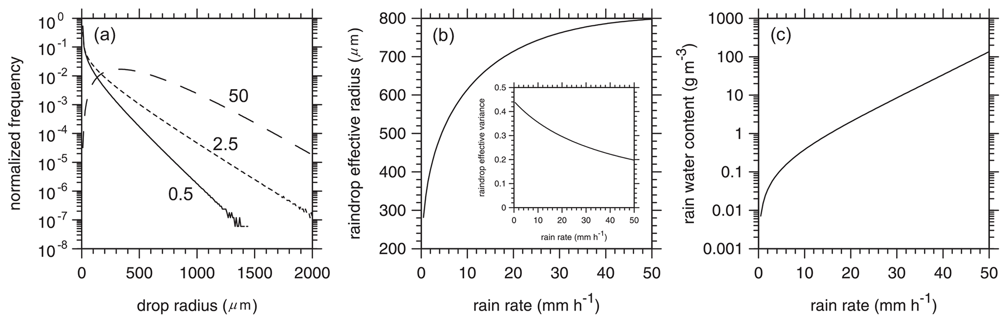
Figure 4 (a) Raindrop size distributions for three values of rain rate (mm h⁻¹). (b) Rain droplet effective radius and variance as functions of rain rate according to the formulation of Ulbrich (1983) and the assumed gamma distribution parameter as discussed in Sect. 4.1.5. (c) Rainwater content as a function of rain rate.

The Mie phase functions that follow from Fig. 4 and Eq. (8) have very pronounced forward peaks that are difficult to capture well in the MC models. Hence, because rain usually resides beneath thick clouds, where radiance fields are highly diffuse, the 3D RT models use p_HG(μ;g).

4.2 Optical properties: underlying surfaces

Snow-free surface albedo over land for visible (0.3–0.7 µm) and infrared (0.7–5.0 µm) SW bands was calculated from climatological bidirectional-reflection distribution function parameters for 16 d periods based on 12 years (2002–2013) of MODIS MCD43GF data (Schaaf et al., 2002). Terrestrial snow albedo data for the same spectral bands are based on Moody et al. (2007), whose calculations were, in turn, based on 5 years (2000–2004) of climatological statistics of Northern Hemisphere white-sky albedos for 16 International Geosphere–Biosphere Programme (IGBP) ecosystem classes when accompanied by the presence of snow on the ground. For ice-covered land or water surfaces, BB-averaged albedos over 16 000–50 000 cm⁻¹ are provided by X-MET (via ECMWF).

Ideally, the 3D RT models should include bidirectional-reflection and bidirectional-emission functions, such as the land surface model of Rahman et al. (1993), which is in EarthCARE's SW 3D RT code, but global parameters are lacking. Hence, spectral albedos, as just described, and the Lambertian assumption are used.

For open water surfaces, spectrally independent ocean albedo is approximated by

$$\begin{array}{}\text{(11)}& \begin{array}{rl}{\mathit{\alpha }}_{\mathrm{sfc}}=& \mathrm{0.021}+x^{\mathrm{2}}(\mathrm{0.0421}+x(\mathrm{0.128}+x(-\mathrm{0.04}+x\\ & \left({\displaystyle \frac{\mathrm{3.12}}{\mathrm{5.68}+w}}\right)+{\displaystyle \frac{\mathrm{0.074}{x}^{\mathrm{2}}}{\mathrm{1}+\mathrm{3}w}}\left)\right)),\end{array}\end{array}$$

where $x=\mathrm{1}-\cos {\mathit{\theta }}_i$, θ_i is zenith angle of an incident photon, and w is surface wind speed (m s⁻¹) (Hansen et al., 1983). The 3D SW model uses Eq. (11) for all photons arriving at a water surface. Additionally, it uses the ergodic wave model of Cox and Munk (1956) to describe the probability of a SW photon incident at the surface being reflected, with the probability defined by Eq. (11), toward a BBR telescope. As such, simulated radiances capture some semblance of sun glint, the effects of which are tempered by EarthCARE's orbit (Illingworth et al., 2015).

While the 1D SW model uses Eq. (11), with θ₀ replacing θ_i, to describe direct-beam albedo, its diffuse-beam albedo is

$$\begin{array}{}\text{(12)}& 〈{\mathit{\alpha }}_{\mathrm{sfc}}〉=\mathrm{0.03815}+{\displaystyle \frac{\mathrm{0.1486}}{\mathrm{5.68}+w}}+{\displaystyle \frac{\mathrm{0.0026}}{\mathrm{1}+\mathrm{3}w}},\end{array}$$

which is just the integral of Eq. (11) assuming isotropic irradiance, regardless of sky condition. Last, hemispheric spectral emissivities for land and sea surfaces, for each RRTMG_LW band, are based on Huang et al. (2016). Like albedo, emissivity is assumed to be Lambertian.

4.3 One-dimensional radiative transfer modelling

The 1D RT models in RRTMG are meant to be applied to layered atmospheres with optical properties varying only in the vertical. As RRTMG was designed for use in large-scale models, it comes with algorithms that address unresolved horizontal fluctuations in cloud water content and cloud overlap. These algorithms are not needed for EarthCARE because RRTMG will be applied to individual JSG columns resolved at ∼1 km resolution with homogeneous layers.

The LW transport solver in RRTMG performs flux calculations for a single diffusivity angle with an adjustment for profiles that contain large H₂O vapour content. It is an emissivity model that neglects scattering by all atmospheric constituents. Its SW solver employs the multi-layer delta-Eddington two-stream approximation (Wiscombe, 1977), which accounts for multiple scattering but, as with the LW solver, has well-documented conditional limitations for aerosol and cloud conditions (e.g., Li and Ramaswamy, 1996; Barker et al., 2015a). Nevertheless, due to RRTMG's widespread use at the time of writing, it is used for EarthCARE with a minimum of alterations so as to be consistent with other current applications.

There are three applications of the 1D SW and LW RT models to each valid JSG column along the retrieved cross-section. The first, denoted as “all-sky”, uses the full retrieved profiles. The second is “clear-sky”, where clouds are removed, leaving molecules and aerosols. The third application is “pristine-sky”, in which clouds and aerosols are removed, leaving just the molecular atmosphere.

4.4 Three-dimensional radiative transfer modelling

Monte Carlo solutions of the 3D RT equation are used to calculate both SW and LW fluxes and radiances. This represents a break from, and advancement over, previous satellite missions that have been limited to the use of 1D RT solvers. The 3D RT models are discussed in the following subsections.

4.4.1 SW radiation

Solar fluxes and radiances are computed by a local estimation-based Monte Carlo algorithm (Marchuk et al., 1980; Barker et al., 2003). It is discussed here in general terms, except for aspects that have not been published or were designed specifically for EarthCARE.

Unlike the 1D RT models that act on individual columns, 3D RT models require collections of columns. Photons get injected uniformly across D⁺'s that are expected to be at most ∼60 km along-track by ∼30 km across track (see Fig. 2). The cosine of the solar zenith angle μ₀ is uniform over D⁺ and set by its central pixel. Total numbers of injected photons per domain are to be determined, as they depend on computational resources, acceptable Monte Carlo sampling noise for either fluxes or radiances, and areal extents of individual D⁺'s. The number of photons injected per spectral band is proportional to the weight associated with quadrature points in RRTMG's CKD model.

Each atmospheric cell has a spectral cumulative extinction vector whose entries for attenuating constituents are ordered, for efficiency, as ice cloud, liquid cloud, Rayleigh scatterers, absorbing gases, aerosols, and rain. When an interaction between an attenuator and a photon takes place, a uniform random number between 0 and 1 is generated, and the (normalized) extinction vector is searched sequentially, thus setting the attenuator, with its single-scattering properties used to establish whether absorption or scattering takes place (cf. Barker et al., 2003). When a scattering event occurs, a fraction 1−ω₀ of the photon's weight goes into local heating. What remains has its weight reduced by a factor of ω₀.

At each scattering event, the probability of photons being redirected toward a BBR telescope is determined using p(μ). Transmittance through total optical depth between the scattering event and satellite sets the probability of scattered photons reaching the satellite; as this distance is large, and the telescope's aperture small, any path deviation is assumed to result in undetected photons. These contributions are summed to produce final estimates of BBR radiances.

The local estimation method runs into trouble when photons travelling directly toward a telescope undergo a scattering event by cloud particles whose p(μ) values have sharp diffraction peaks (Iwabuchi, 2006). Such rare contributions are valid, but they catastrophically elevate uncertainties, which are difficult to counter with large numbers of “typical” contributions when the number of injected photons is small, as for EarthCARE. A simple way to help without impacting fluxes and HRs is to use the tabulated exact p(μ) to determine all photon forward trajectories, but only those radiance contributions from the first N_Mie scattering events by cloud particles. Thereafter, the blunt-nosed p_HG(μ;g) is used to compute radiance contributions (see Barker et al., 2003).

The rationale behind this approximation is that low-order scatterings that contribute to BBR radiances come largely from p(μ<0), and because they do not spike radiances, several of them are allowed so as to capture details of p(μ). For optically thin clouds there will be few scattering events, and so calls to p_HG(μ;g) will be rare. For thicker clouds, however, after approximately three scatterings photons will have had a fair chance of being redirected onto upward-travelling trajectories that can spike radiances. EarthCARE uses N_Mie=4 for, as shown in Sect. 5.2, it strikes a balance between bias and random radiance errors (Barker et al., 2003).

When a photon arrives at the surface, it undergoes Lambertian reflection for albedo α_s with 1−α_s of its weight removed and added to net surface irradiance. The probability of being scattered by a surface toward a BBR sensor follows Lambertian reflectance for land, ice, and snow and Cox and Munk (1956) for open water (see Sect. 4.2).

A unique memory-saving aspect of EarthCARE's SW and LW 3D RT models is that the 3D atmosphere never appears explicitly in them. This is because all columns in D⁺ exist along the retrieved cross-section; optical properties of columns off this plane come from a donor column in it, as dictated by ACMB-3D's scene construction algorithm (Barker et al., 2011; Qu et al., 2023).

4.4.2 LW radiation

Longwave radiances are computed efficiently with the backward Monte Carlo technique (Walters and Buckius, 1992; Modest, 2003). The implementation of Cole (2005) is used for EarthCARE. Much of the code resembles that of the SW Monte Carlo, and so discussion is focused on its unique aspects.

Unlike the SW Monte Carlo, photons are not injected uniformly onto the top of D⁺ since the domain itself is the source. Rather, reciprocity of paths from an emission source to a sensor is assumed to hold (Case, 1957). Hence, photons trace back from the top of the assessment domain to their source of emission, where the contribution to radiance is computed using local temperature and optical properties. This process is repeated for each point in the assessment domain and radiance view angle. To reduce the number of rays traced, which is often the main computational expense, rather than trace a unique ray for each quadrature point in the CKD model, it is assumed that scattering optical properties are the same for all quadrature points in a single wavelength interval.

For a given wavelength interval in the CKD model a band-representative photon path is traced backward from the top of the domain to determine a scattering path that can be related to each photon injected for each quadrature point in the band. The photon travels straight through the domain until it has accumulated sufficient scattering optical depth to scatter in the atmosphere or scatter due to an interaction with the surface. Scatter within the atmosphere is determined based on the cumulative distribution of scattering extinction, similar to that in the SW algorithm. For each quadrature point in the CKD wavelength interval, a random number is determined which sets the optical depth that must be accumulated to have an absorption event. Absorption optical depth is accumulated along the path until the photon undergoes an absorption event, at which point (1−ω₀)B(T) is added to the radiance, where B(T) is integrated Planck function, and T is temperature. If, however, the photon reaches the surface, a uniform random number is used to determine if there is absorption by the surface. If the random number is less than surface emissivity ε the radiance is incremented by B(T_s), where T_s is the surface temperature. Otherwise, the path is reflected.

Upward thermal flux at a potentially variable reference height is also computed. This is done using a method similar to that used for radiances, the main difference being the selection (i.e., random generation) of the direction of each ray injected into the domain from the reference height. Once the ray direction is selected, accumulation of emission contributions is the same as it is for radiances.

4.4.3 Estimation of Monte Carlo uncertainty

For a fixed domain, 1D RT models produce single deterministic solutions. Monte Carlo algorithms, however, yield a sample from a distribution. In general, the breadth of the distribution, or Monte Carlo uncertainty, depends on the number of injected photons, the variable being diagnosed, and the geometric and optical properties of the field.

Monte Carlo uncertainties are estimated by explicitly producing M samples of a random variable x, each using N_s photons and initialized with a unique, uniformly distributed random number. Estimated population mean is simply

$$\begin{array}{}\text{(13)}& {\widehat{\mathit{\mu }}}_x\left(M,N_{\mathrm{s}}\right)={\displaystyle \frac{\mathrm{1}}{M}}\sum _{m=\mathrm{1}}^{M}x\left(m,N_{\mathrm{s}}\right),\end{array}$$

where x(m,N_s) is the mth realization of x. From the central limit theorem,

$$\begin{array}{}\text{(14)}& \underset{M\to \mathrm{\infty }}{lim}p\left[\left|{\displaystyle \frac{{\widehat{\mathit{\mu }}}_x\left(M,N_{\mathrm{s}}\right)-{\mathit{\mu }}_x}{\frac{{\mathit{\sigma }}_x\left(M,N_{\mathrm{s}}\right)}{\sqrt{M}}}}\right|\le a\right]={\displaystyle \frac{\mathrm{1}}{\sqrt{\mathrm{2}\mathit{\pi }}}}\underset{-a}{\overset{a}{\int }}{e}^{-u^{\mathrm{2}}/\mathrm{2}}\mathrm{d}u,\end{array}$$

where μ_x and σ_x are the mean and standard deviation of the population from which samples are drawn. Letting ${\widehat{\mathit{\sigma }}}_x\left(M,N_{\mathrm{s}}\right)$ be an estimate of σ_x based on M samples, Monte Carlo “uncertainty” is defined as 1 standard deviation under a Gaussian distribution of samples. This amounts to setting a=1 in Eq. (14) and implies that after M realizations, ${\widehat{\mathit{\mu }}}_x$ has a 68 % chance of lying in

$$\begin{array}{}\text{(15)}& \left[{\widehat{\mathit{\mu }}}_x\left(M,N_{\mathrm{s}}\right)-{\displaystyle \frac{{\widehat{\mathit{\sigma }}}_x\left(M,N_{\mathrm{s}}\right)}{\sqrt{M}}},{\widehat{\mathit{\mu }}}_x\left(M,N_{\mathrm{s}}\right)+{\displaystyle \frac{{\widehat{\mathit{\sigma }}}_x\left(M,N_{\mathrm{s}}\right)}{\sqrt{M}}}\right],\end{array}$$

making for an uncertainty of

$$\begin{array}{}\text{(16)}& {\widehat{\mathit{\rho }}}_x\left(M,N_{\mathrm{s}}\right)\approx \pm {\displaystyle \frac{{\widehat{\mathit{\sigma }}}_x\left(M,N_{\mathrm{s}}\right)}{\sqrt{M}}}.\end{array}$$

As M increases, estimates of ${\widehat{\mathit{\sigma }}}_x$ stabilize; they do not go to zero.

5 Results

This section's main purpose is to showcase a sample of EarthCARE's radiation products, some of which are utilized directly for radiative closure assessment, as will be reported in a later study. Results are shown using only ACM-CAP data; corresponding results for ACM-COM's composites are qualitatively the same. Results are shown mainly using data from two test frames: the “Halifax frame”, which passes near Halifax, Canada, and the “Hawaii frame”, which passes near Hawaii (Qu et al., 2022).

As noted in the Introduction, many radiative quantities are averaged over ∼ 100 km² assessment domains. It is expected that these domains will be configured to 21 km along-track by 5 km across-track. This is to strike a balance for closure assessment between limiting the scene construction algorithm's (Qu et al., 2023) impact on radiance and flux estimates and facilitating horizontal transport of photons. To simplify the presentation of results, radiative transfer estimates are shown for a reference height of 20 km (cf. Loeb et al., 2002); in operations they will vary.

5.1 RRTMG 1D fluxes: pristine-, clear-, and all-sky

As discussed in Sect. 2, broadband flux and heating rate profiles for all admissible L2 columns are computed by RRTMG's SW and LW 1D RT models. The left column of Fig. 5 shows ∼ 2200 km of cloud and aerosol properties retrieved by ACM-CAP's synergistic algorithm (Mason et al., 2023). These results pertain to 21 km long non-overlapping assessment domains near the centre of the Halifax test frame. The middle column shows corresponding SW all-sky HRs and differences between all-sky HRs and clear-sky HRs (CRE: cloud radiative effect) as well as clear-sky HRs and pristine-sky HRs (ADE: aerosol direct effect). Aside from the usual 1D RT features, such as large SW heating near the cloud top and much smaller values below relative to clear sky, the only peculiarity is the fairly strong heating at ∼ 5 km altitude at the southern end. This is due to an elevated layer of water vapour. The vast majority of minor heating due to aerosol is from continental pollution that overrides sea salt.

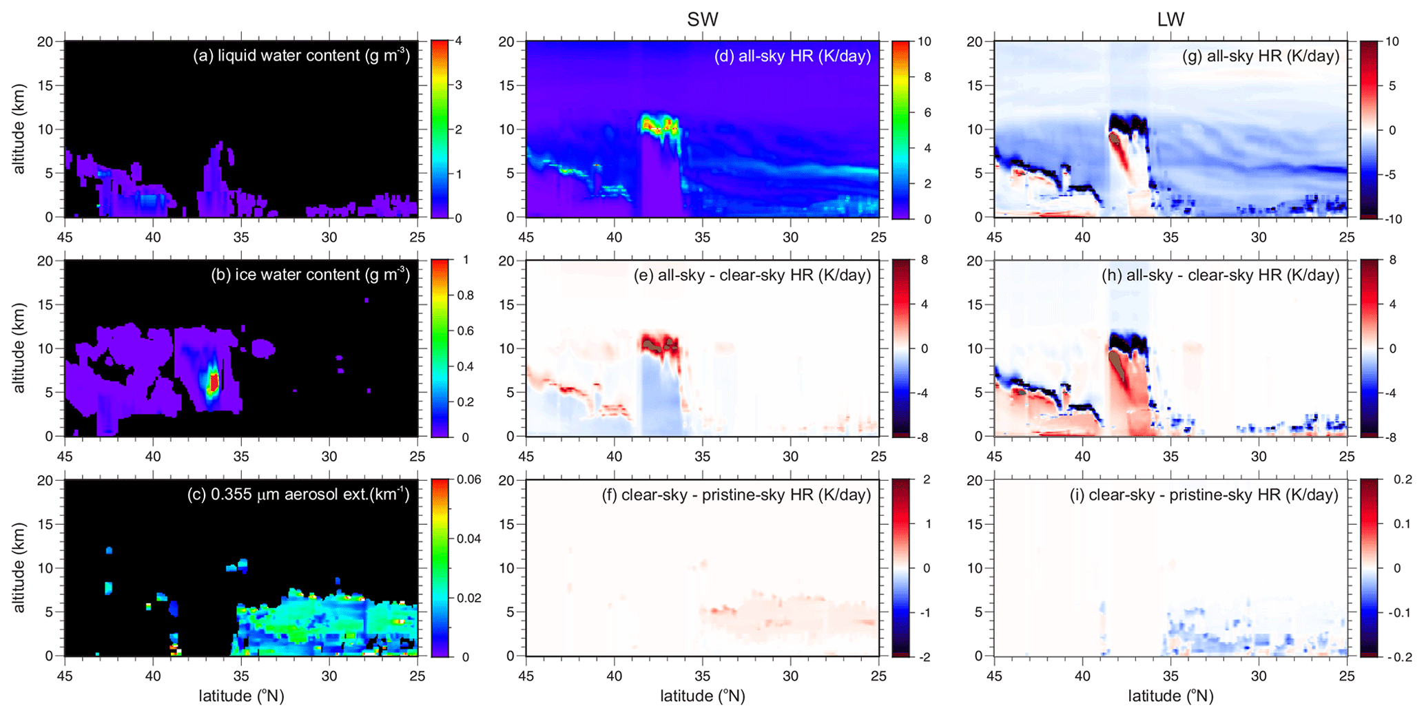
Figure 5 (a) Profiles of domain-average cloud liquid water content, (b) ice water content, and (c) aerosol extinction coefficient for 21 km long assessment domains for the Halifax frame, as inferred by ACM-CAP's synergistic algorithm. (d) Corresponding domain-average, all-sky SW broadband heating rates computed by RRTMG's 1D RT model. (e) Difference between HRs shown in panel (d) and those computed by RRTMG for clear-sky conditions. (f) As in panel (e), except these HR differences are for clear skies and pristine skies. Panels (g), (h), and (i) are as in panels (d), (e), and (f), respectively, except these are for LW broadband heating rates.

The rightmost column in Fig. 5 is like the middle column, but it shows results for LW HRs. As expected, there is strong cooling in the upper 1–2 km or so of clouds, little net heating or cooling below, and general cooling from cloudless skies. LW CREs are generally stronger than in the SW and exhibit strong cooling near all cloud tops and warming in clouds when they are of sufficient vertical extent. LW ADEs are an order of magnitude smaller than their SW counterparts and manifest themselves as cooling just beneath their SW warming counterparts.

To demonstrate what will be available in the ACM-RT archive, Fig. 6 shows TOA CRE, ADE, and some integrated cloud and aerosol properties that correspond to Fig. 5. Some noteworthy points here are SW CRE reaching ∼ 300 W m⁻² at μ₀≈0.3 due to clouds near 41^∘ N with large cloud water paths (CWPs), LW CRE reaching 100 W m⁻² near 37^∘ N due to supercooled liquid aloft, and weak ADE (∼ −10 W m⁻² in the SW and less than 1 in the LW) stemming from aerosol optical depth at 0.355 µm being at most 0.2. Aside from this, there is very little to comment on in these plots; they serve to demonstrate what will be available in the ACM-RT archive.

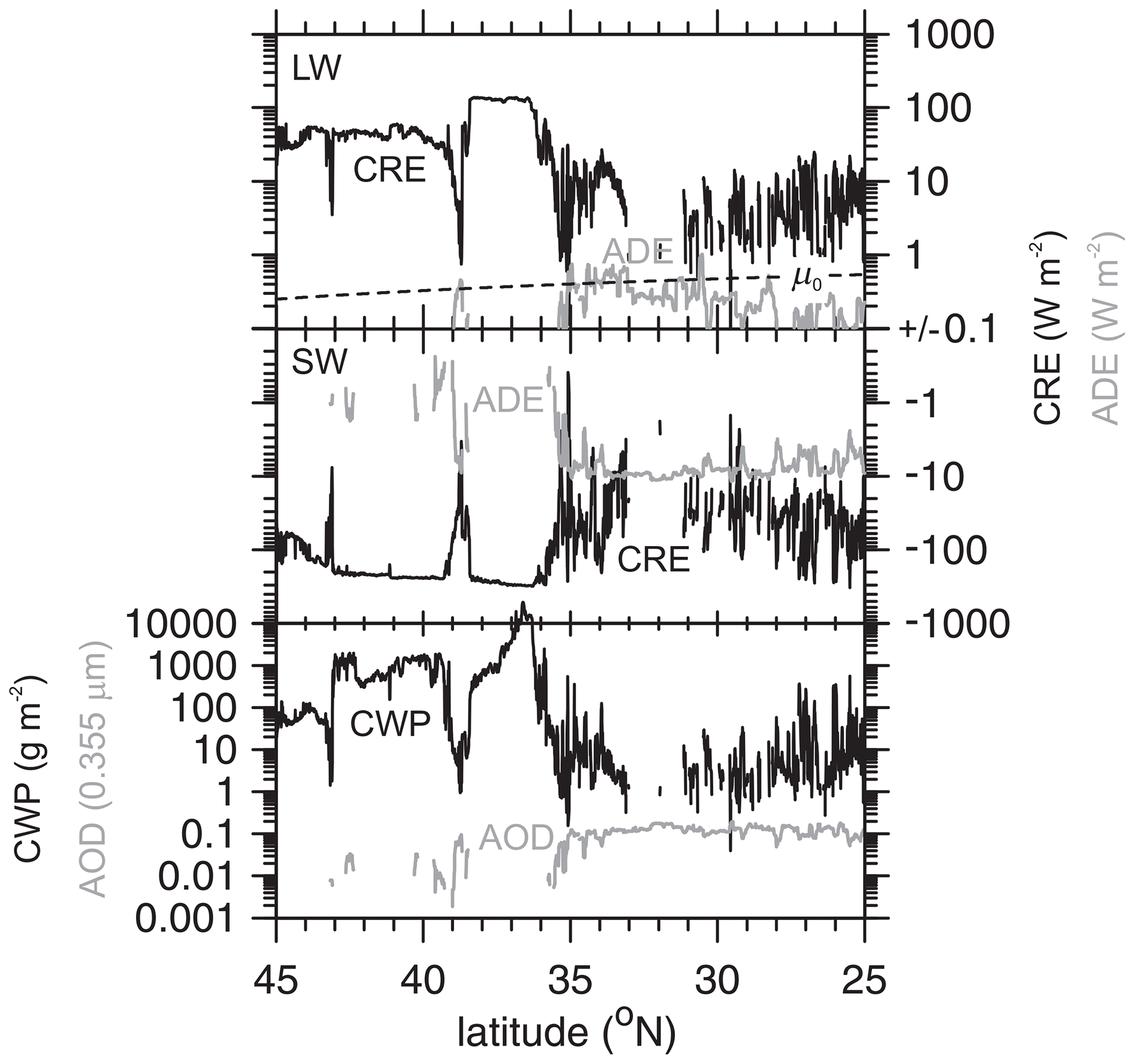
Figure 6 Top panel: cloud radiative effect (CRE) and aerosol direct effect (ADE) as functions of latitude for broadband SW at an altitude of 20 km for 21 km long assessment domains, as shown in Fig. 5. μ₀ is the cosine of the solar zenith angle. Middle panel: as in the top panel, except it is for broadband LW. Lower panel: assessment domain-average cloud water path (CWP) and aerosol optical depth (AOD).

5.2 On the benefits of employing 3D RT models

As mentioned above, one of EarthCARE's notable advancements over prior alike missions is operational use of both 1D and 3D RT models. The decision to use 3D RT models was fuelled by myriad studies that show systematic differences between 1D and 3D treatments of RT, especially for cloudy atmospheres at solar wavelengths. Results shown in this subsection help justify the computational expense of using 3D RT models operationally.

Before getting to results that apply strictly to EarthCARE, consider a detailed view of the impact of neglecting multi-dimensional RT. Figure 7 shows nadir SW radiances simulated by a Monte Carlo RT model (Villefranque et al., 2019) for two stretches of the Hawaii test frame, each measuring 128 km along-track by 20.25 km across-track (Qu et al., 2022). The 3D RT simulation used horizontal grid spacing Δx=0.25 km, while its 1D rendition used Δx set arbitrarily large. Hence, differences in their radiances stem entirely from the dimensionality of the RT solution. For this demonstration, the number of photons per column was 4096, which is, on an areal density basis, several times larger than what will be used operationally for the EarthCARE mission.

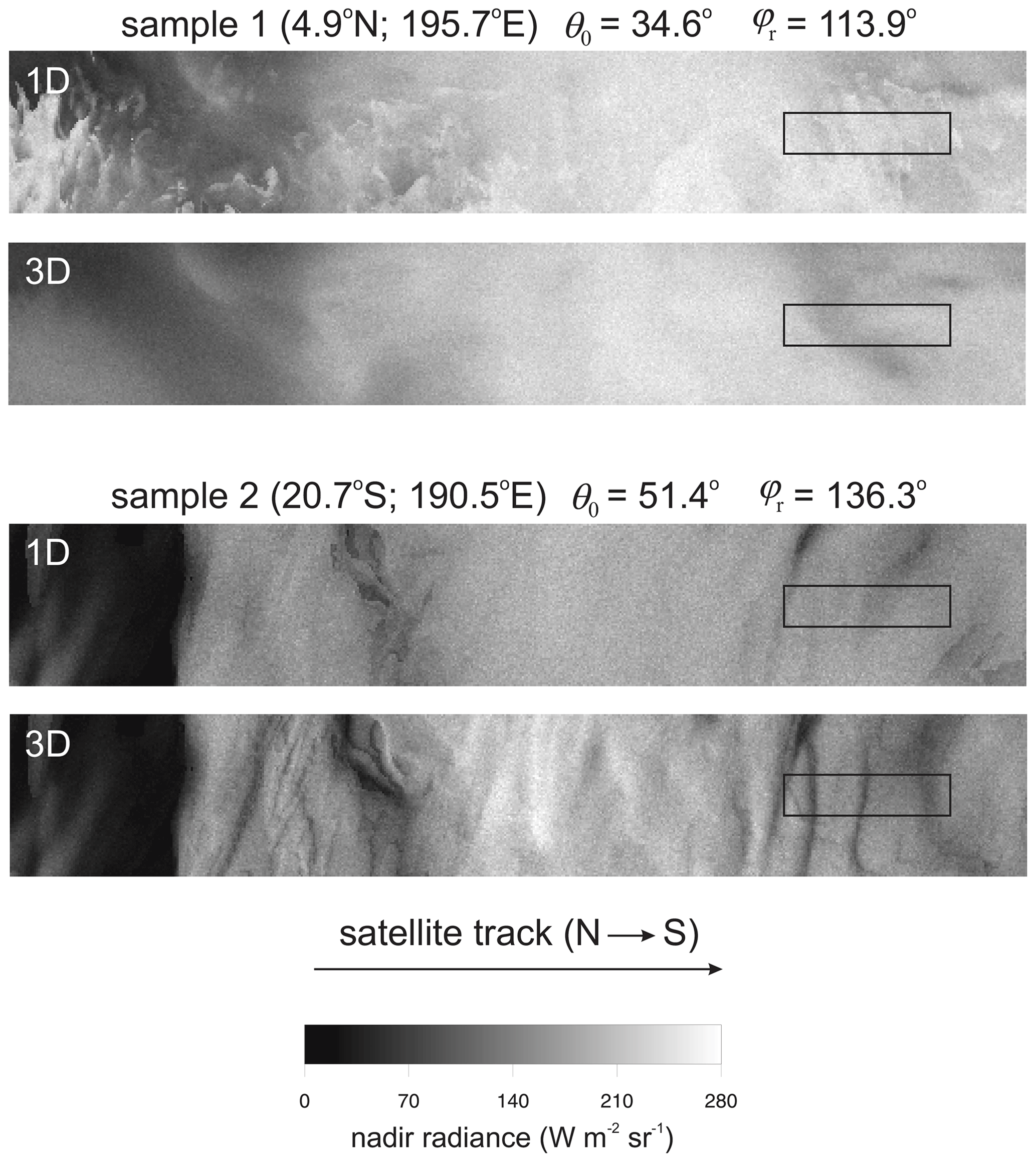
Figure 7 Nadir broadband SW radiances for two sample regions in the Hawaii frame; both regions measure 128 km along-track by 20.25 km across-track. Small rectangles indicate a 5×21 km assessment domain, the size used for radiative closure assessments. Central values of latitude and longitude are listed along with θ₀ and φ_r (measured clockwise from the satellite's tracking direction). The labels 3D and 1D indicate RT model dimensionality using horizontal grid spacings of 0.25 km and 10⁶ km.

These images display the varied and complicated ramifications for radiances when 1D RT modelling theory is assumed to apply. For sample 1, 1D radiances show much variability and sharp contrasts relative to their 3D counterparts; off-nadir views (not shown) look much the same. This region is blanketed by thick overcast ice clouds, which at Δx=0.25 km act to diffuse upwelling radiation, thus blurring localized reflection from low-level intermittent liquid clouds (e.g., Diner and Martonchik, 1984). When 1D RT is affected by setting Δx large, however, flow of radiation is confined to the vertical, and the sharp features of liquid clouds remain intact regardless of altitude.

On the other hand, sample 2 has mostly low- to mid-level liquid clouds and shows, due in part to large θ₀, more familiar differences between 3D and 1D RT (e.g., Barker et al., 2017). In particular, 1D radiances lack texture, whilst their 3D counterparts exhibit much contrast due to shadowing and cloud-side illumination. Note, however, that imagery for thin liquid clouds at the northern edge of the sample depends little on Δx. This is because reflected photons undergo small numbers of scattering events and thus tend to exit clouds close to where they enter.

Consider now differences one can encounter in applications to EarthCARE retrievals. Figure 8 shows differences between 3D and 1D RT modelled SW broadband upwelling fluxes at 20 km and surface irradiances for 5×21 km assessment domains across the Hawaii frame using ACM-CAP cloud properties. Values for 3D and 1D RT are from the Monte Carlo model using Δx=1 km and arbitrarily large Δx, respectively. Each simulation used 2.5×10⁶ photons, which is likely much larger than what will be used operationally throughout the mission. For almost cloud-free skies, thin ice clouds only with ice water path IWP <0.01 kg m⁻², and very thick clouds with CWP >0.5 kg m⁻², differences are well within ±10 W m⁻² for fluxes at both levels. Clearly, under these conditions SW photon trajectories are characterized by either extremely small or large numbers of scattering events with cloud particles for both 1D and 3D RT. For the majority of other cloud conditions, however, especially with CWP in the vicinity of ∼ 0.1 kg m⁻², differences can be much larger than ±30 W m⁻², which far exceeds EarthCARE's goal (ESA, 2001; Illingworth et al., 2015; Eisinger et al., 2023), the implication being that many attempts to perform a radiative closure assessment on EarthCARE's retrievals will be doomed to failure if 1D RT models are adhered to.

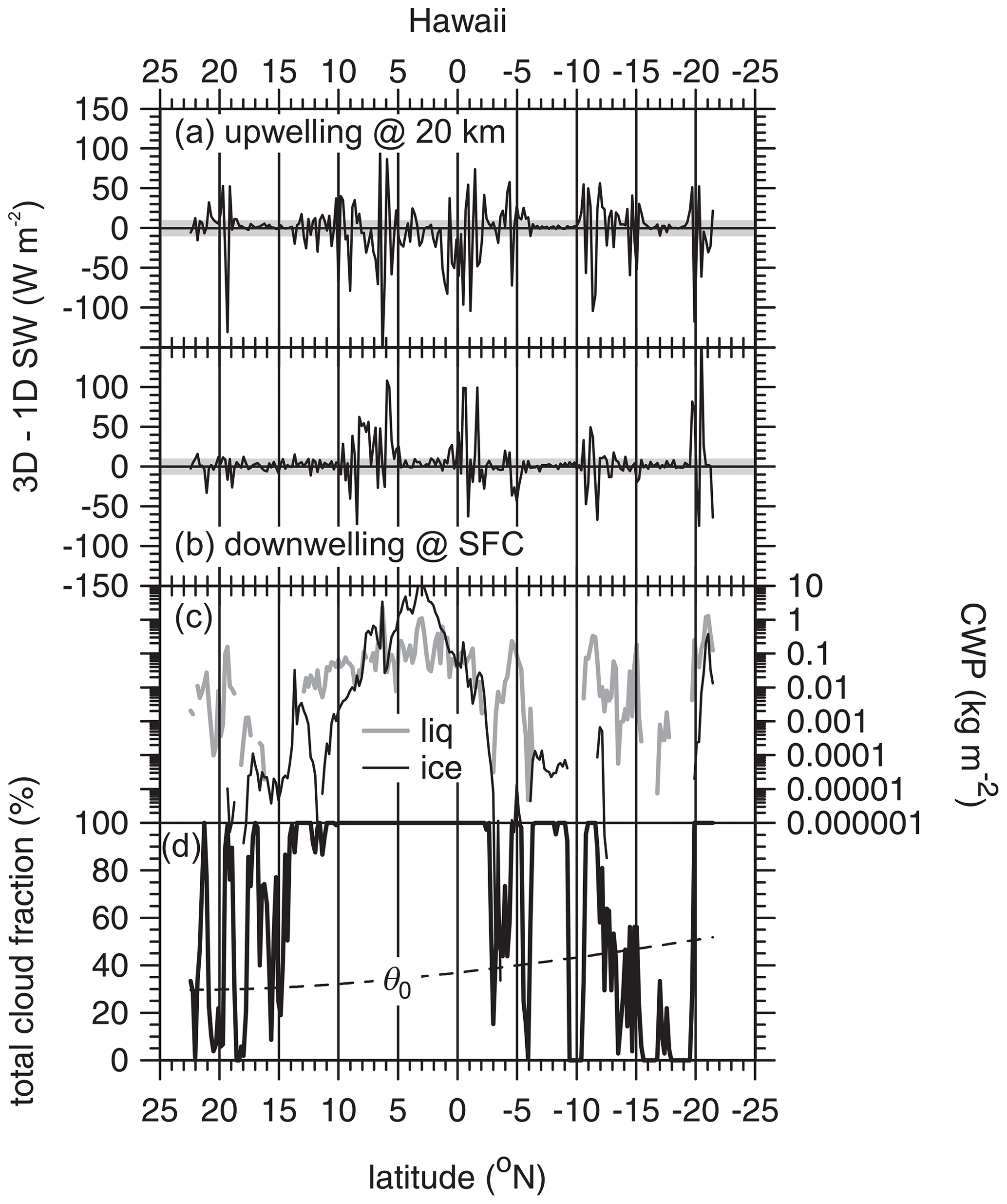
Figure 8 (a) Difference between upwelling SW fluxes at an altitude of 20 km as predicted by 3D and 1D RT models for 5×21 km assessment domains of the Hawaii frame. The shaded area indicates EarthCARE's goal of ±10 W m⁻². (b) As in panel (a), except this is for SW surface irradiance. (c) Mean liquid and ice cloud water paths for the Hawaii frame's 5×21 km domains. (d) Corresponding total cloud fraction and solar zenith angle for the same assessment domains.

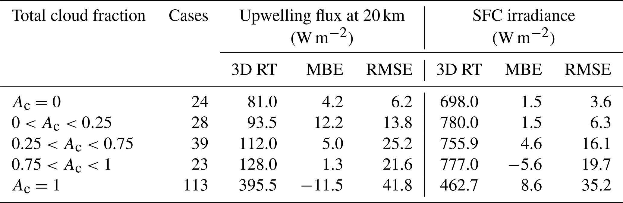
Figure 9 shows cumulative frequency distributions of the differences shown in Fig. 8 for several ranges of total cloud fraction A_c. For upwelling fluxes at 20 km with A_c<0.25, median differences are all close to zero. The same goes for 3D–1D mean bias errors (MBEs), as listed in Table 2. Differences tend to be distributed more or less symmetrically about zero with occasional large differences, exceeding ±50 W m⁻², enhancing root mean square errors (RMSEs) as A_c increases (see Table 2) relative to the 16th and 84th percentiles of the distributions, which can be gleaned from the graphs.

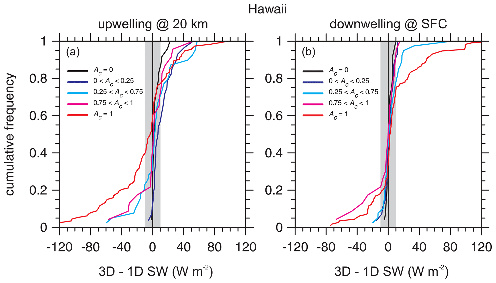
Figure 9 (a) Cumulative frequency distributions for differences between 3D and 1D Monte Carlo RT model estimates of upwelling SW flux at an altitude of 20 km for 5×21 km assessment domains for the Hawaii frame partitioned according to the assessment domain total cloud fraction A_c (see Table 2 and Fig. 8). The shaded area indicates EarthCARE's goal of ±10 W m⁻². (b) As in panel (a), except these are for surface (SFC) irradiances.

Table 2 Mean 3D SW RT values, mean bias errors (MBEs), and root mean square errors (RMSEs) for corresponding 3D–1D RT results (see Figs. 8 and 9) for 5×21 km assessment domains for the Hawaii frame and several ranges of total cloud fraction A_c.

There are at least two interesting points to these plots that involve extreme cloud conditions. First, 3D–1D can be expected to be maximized for overcast domains, which implies that the geometry of overcast clouds is often anything but approximately plane-parallel and homogeneous (cf. Hogan et al., 2019). Second, for assessment domains (D's) with A_c=0, 3D–1D values for upwelling flux at 20 km show a tendency to be positive on account of contributions from clouds in the surrounding buffer zone (see Fig. 2).

Figure 10 shows that SW HR differences between 3D and 1D RT for the Hawaii frame's 5×21 km assessment domains are much less dramatic than those seen in Figs. 8 and 9 for boundary fluxes. At all altitudes and ranges of A_c, MBEs are essentially zero and close in magnitude to Monte Carlo uncertainties for 2.5×10⁶ photons. There are several reasons why RMSE values are ∼10 times larger than Monte Carlo uncertainties and only increase slightly as A_c increases. There are the obvious differences due to cloud-side illumination, shadowing, and photon entrapment (Hogan et al., 2019), as well as impacts on flux profiles for 3D RT due to out-of-domain sources and sinks of photons, i.e., clouds outside D, but still in D⁺, that cast shadows or scatter radiation into D.

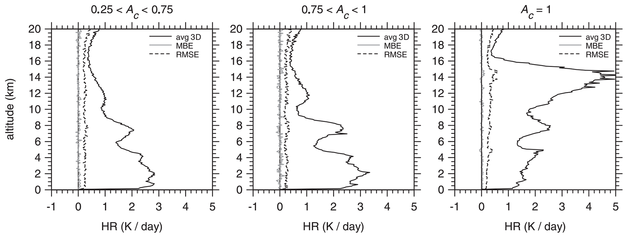
Figure 10 Mean 3D RT SW heating rate (HR) profiles for 5×21 km assessment domains for the Hawaii frame partitioned according to the assessment domain total cloud fraction A_c (see Fig. 8). Also shown are mean bias errors (MBEs) and root mean square errors (RMSEs) between 3D and 1D RT models. The number of cases per A_c range is listed in Table 2.

There is the possibility that radiative closure assessments of cloud and aerosol retrievals could (i.e., should) use broadband radiances rather than fluxes. There are reasons both for and against this. For instance, off-nadir BBR radiances offer powerful assessments due to their weak correlation, relative to nadir BBR radiances, with MSI radiances that are used for some retrievals. They can, however, arise from attenuators outside the domain being assessed (see Barker et al., 2015b). On the other hand, all of EarthCARE's performance goals are in terms of BBR fluxes, which will be estimated regularly by tailor-made algorithms (Velázquez-Blázquez et al., 2023a) despite adding at times substantial uncertainty at the last step of EarthCARE's processing chain.

Regardless, SW BBR radiances will be estimated throughout the mission. Figure 11 shows nadir values for the Hawaii frame's assessment domains using 2.5×10⁶ photons per assessment domain and Δx=1 km. It also shows relative Monte Carlo uncertainties for N_Mie=4 and N_Mie→∞. As 2.5×10⁶ photons per domain is likely to be more than routine operations can afford, uncertainties for N_Mie→∞ could be substantially larger than those shown here. This would render them useless for most assessments. While use of N_Mie=4 will help, as is evident for the thick clouds between 0 and 10^∘ N and near 20^∘ S, it will foster errors in radiances themselves. Two options are being considered: (i) using radiances instead of fluxes for assessments when their relative Monte Carlo uncertainties are less than some specified value (e.g., 0.01; see Fig. 11) and (ii) unbiased variance reduction methods (e.g., Iwabuchi, 2006).

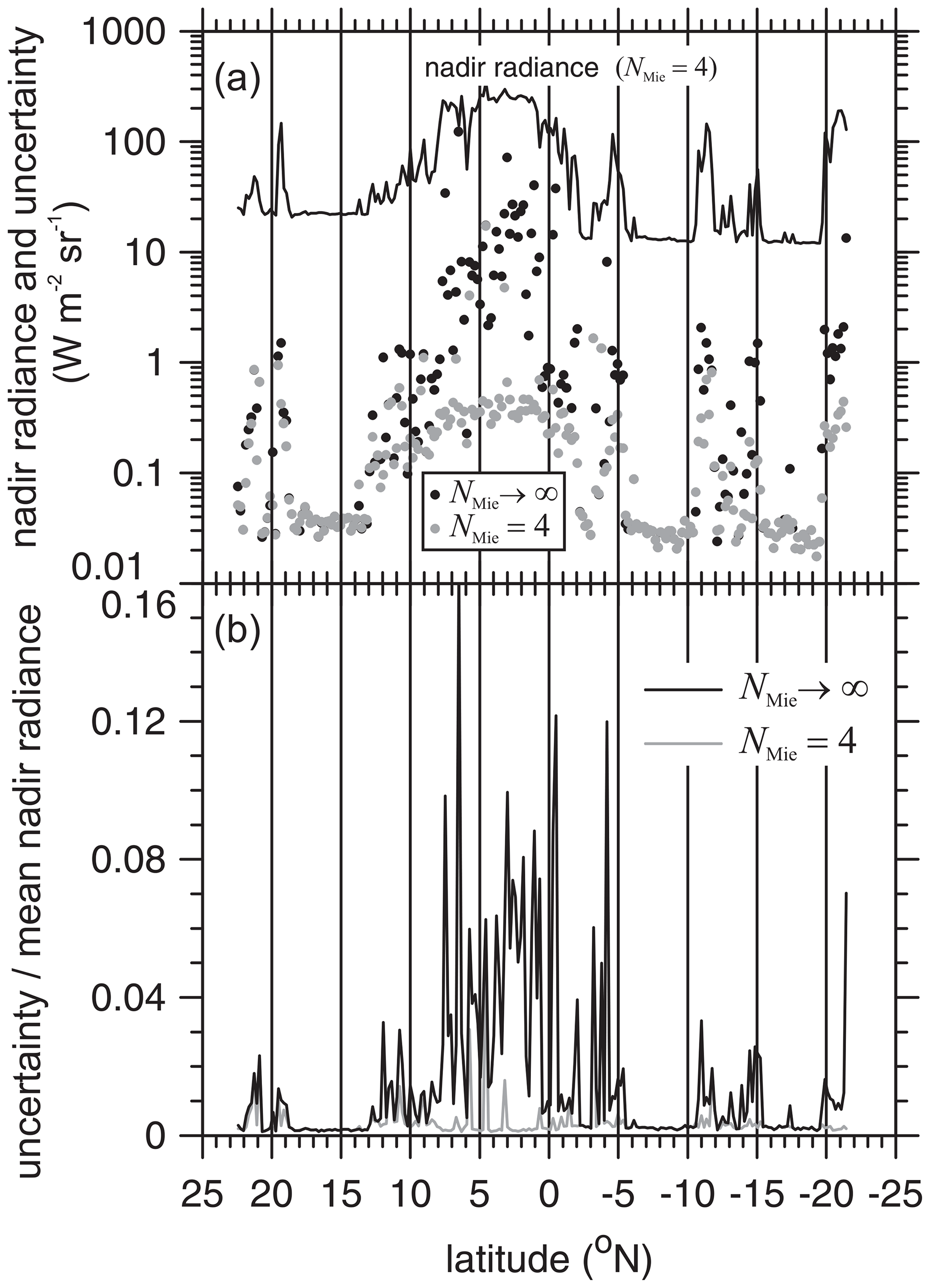
Figure 11 (a) The line shows 3D RT nadir broadband radiances using Δx=1 km when reverting to the Henyey–Greenstein phase function p_HG after N_Mie=4 cloud-particle-scattering events for 5×21 km assessment domains of the Hawaii frame. Dots are Monte Carlo uncertainties when p_HG is never used (N_Mie→∞) and when it is used after four cloud scattering events (N_Mie=4). (b) Using data in panel (a), Monte Carlo domain-average uncertainties relative to mean values for both values of N_Mie. Each domain received 2.5×10⁶ photons.

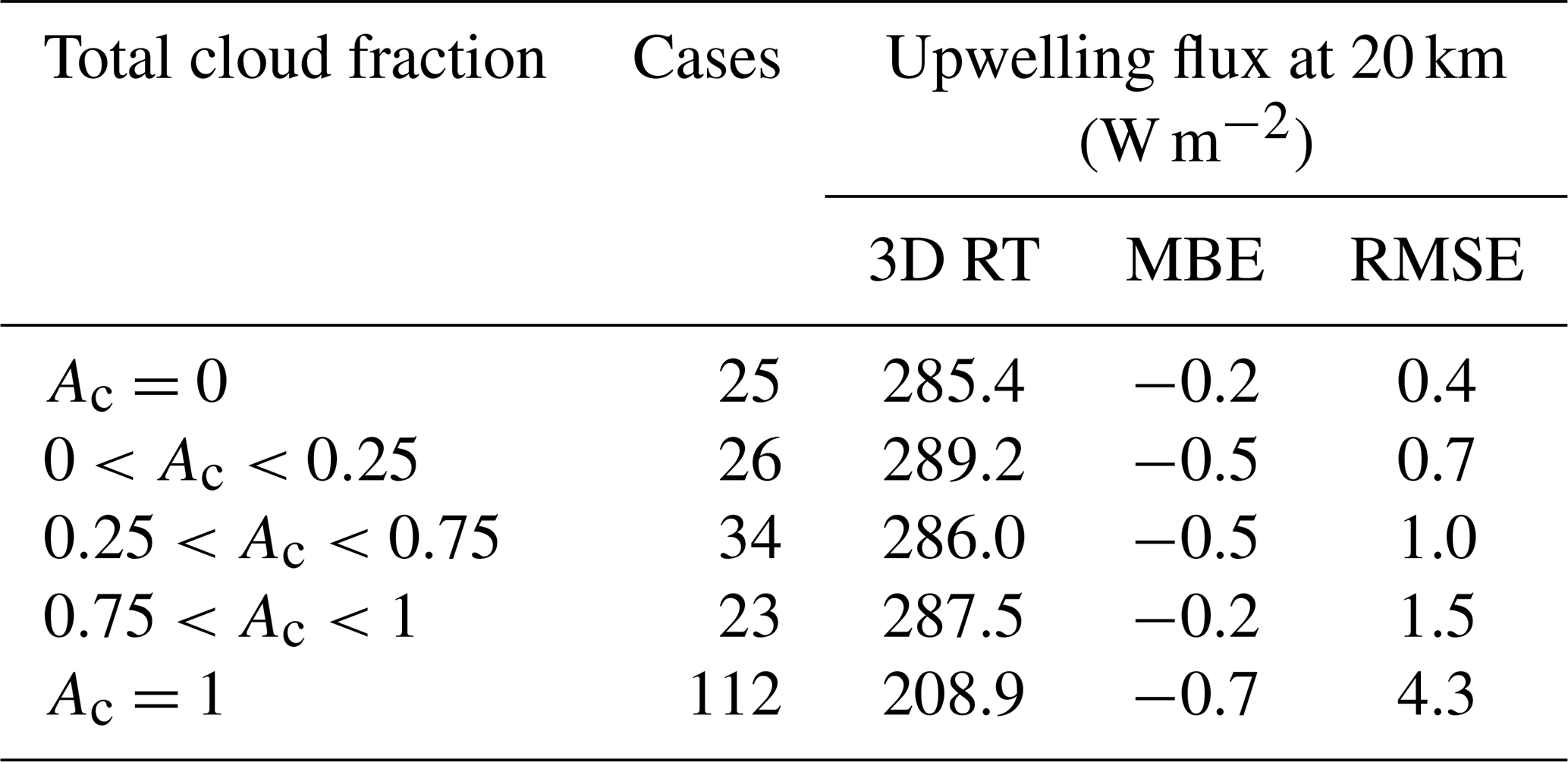
As is well known, flux and radiance differences between 3D and 1D treatments of RT for LW radiation are usually much smaller than those for SW radiation (e.g., Ellingson and Takara, 2005; Cole et al., 2005; Hogan et al., 2016; Fauchez et al., 2017). Figure 12 shows the LW counterpart of the upper panel in Fig. 8. When differences go beyond ±10 W m⁻², they do so along with corresponding large differences in SW fluxes, typically for overcast skies with CWP ∼ 0.1 kg m⁻². As shown in Fig. 13, ∼ 5 % of overcast cases exhibit 3D fluxes that are less than their 1D counterparts by more than 10 W m⁻². For these domains, CWPs are small relative to their neighbouring domains. This demonstrates a difficulty when interpreting “fluxes” for 5×21 km domains: at 20 km altitude, fluxes for 3D RT can be influenced substantially by adjacent cloudier domains. Table 3, however, shows that 3D and 1D fluxes usually differ by less than ±1 W m⁻², which is on the order of the Monte Carlo uncertainty for these calculations, roughly 0.2 W m⁻².

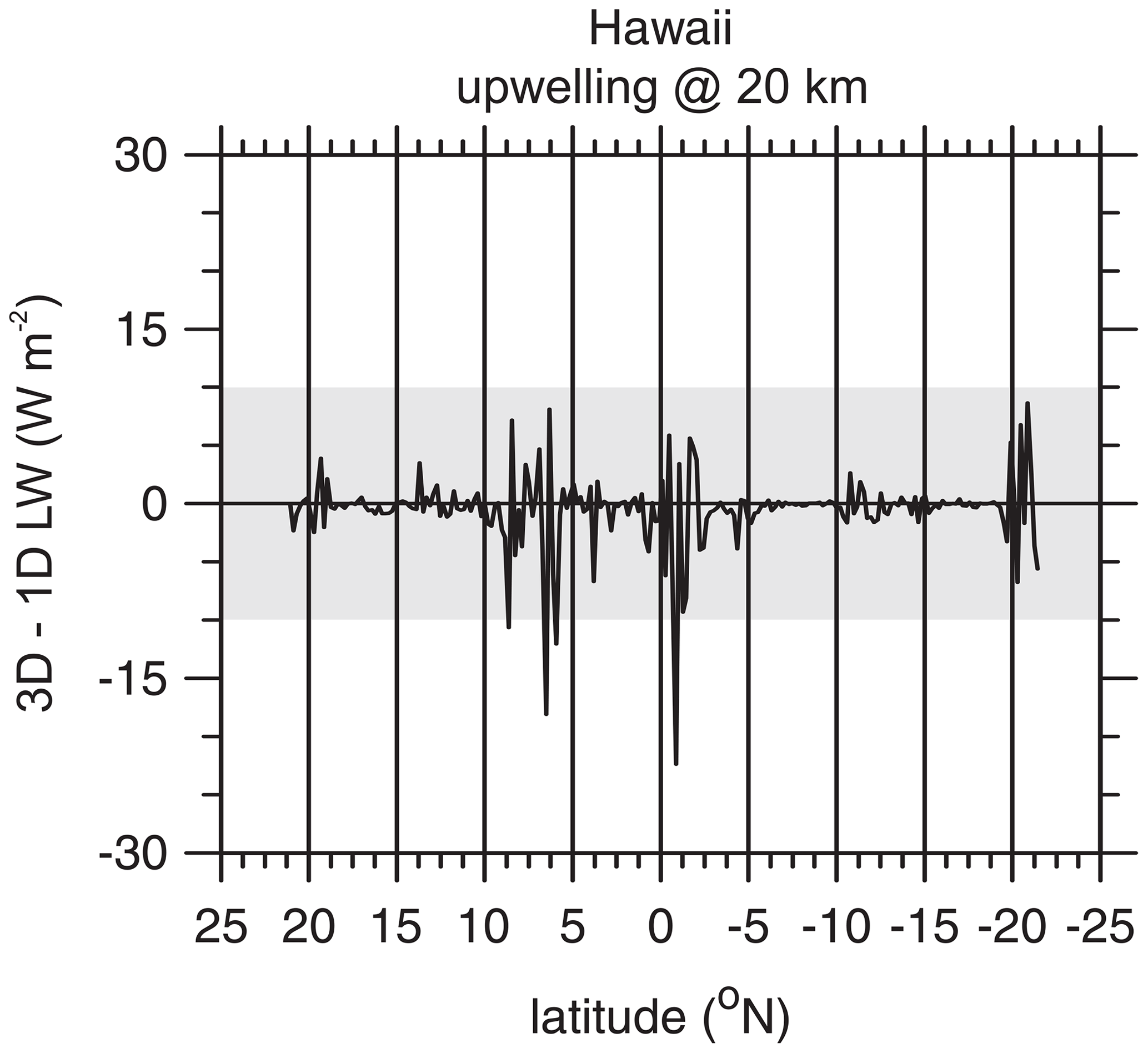
Figure 12 Difference between upwelling LW fluxes at an altitude of 20 km as predicted by 3D and 1D RT models for 5×21 km assessment domains of the Hawaii frame. A positive value means that 3D upwelling flux exceeds its 1D counterpart. The shaded area indicates EarthCARE's goal of ±10 W m⁻².

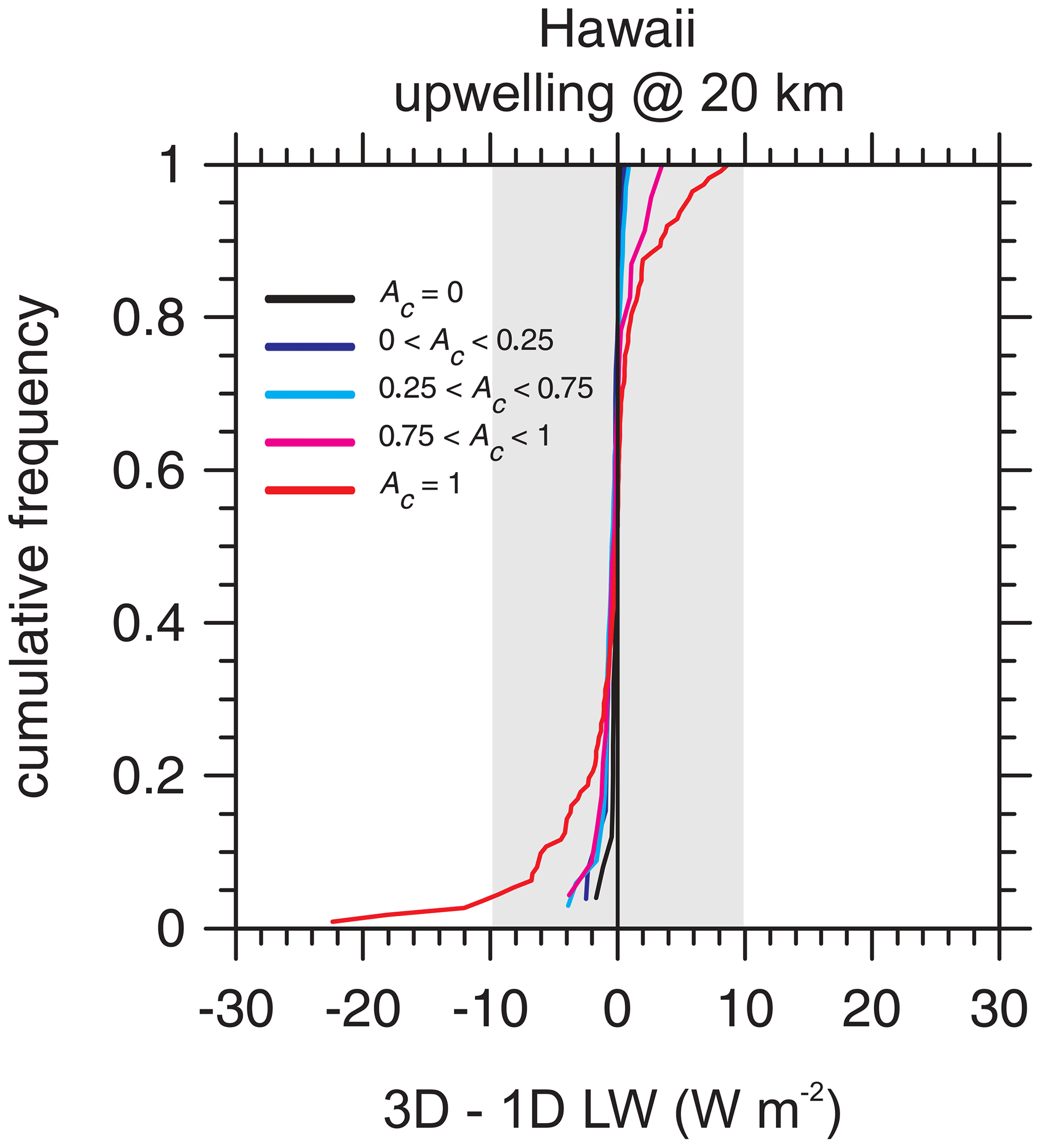
Figure 13 Cumulative frequency distributions for differences between 3D and 1D RT model estimates of upwelling LW flux at an altitude of 20 km for 5×21 km assessment domains for the Hawaii frame partitioned according to the assessment domain total cloud fraction A_c (see Table 3). The shaded area indicates EarthCARE's goal of ±10 W m⁻².

Table 3 Mean 3D LW RT values, mean bias errors (MBEs), and root mean square errors (RMSEs) for corresponding 3D–1D RT results (see Figs. 8 and 9) for 5×21 km assessment domains for the Hawaii frame and several ranges of total cloud fraction A_c.

6 Summary

The EarthCARE satellite mission's objective is to retrieve profiles of aerosol and water cloud physical properties from measurements made by its cloud-profiling radar (CPR), backscattering lidar (ATLID), and passive multi-spectral imager (MSI). While several L2a processes infer geophysical properties using measurements from a single sensor (see several articles in this special issue), EarthCARE's primary product comes from the L2b synergistic retrieval algorithm in ACM-CAP (Mason et al., 2023). These retrievals, together with other geophysical properties obtained from either pre-existing satellite data or real-time weather prediction models, are input into broadband (BB) radiative transfer (RT) models that predict radiances and fluxes commensurate with measurements made and inferred from EarthCARE's BB radiometer (BBR). The scientific goal is that modelled and “observed” BB fluxes differ, on average, by less than ±10 W m⁻².

This report describes the BB RT models used for EarthCARE and their products, which together comprise the ACM-RT process. Shortwave (SW) and longwave (LW) flux and heating rate (HR) profiles are computed by a 1D solver, based on RRTMG, for each ∼ 1 km nadir column of inferred properties. In addition to the 1D RT models, which are ubiquitous to almost all operational and research satellite missions, EarthCARE is the first to employ 3D (Monte Carlo) RT models operationally. Both SW and LW models will compute radiances for the BBR's three viewing directions, with the SW model also computing flux and HR profiles. The 3D LW model produces only upwelling fluxes at a variable reference level, as dictated by the BMA-FLX process (Velázquez-Blázquez et al., 2023a). All 3D RT products are averages over 5×21 km assessment domains that are constructed in the ACMB-3D process (Barker et al., 2023) using a radiance mapping algorithm and MSI data (Barker et al., 2011).

When the ACM-CAP process runs successfully, its retrievals are operated on by the RT models. Failing this, the RT models are applied to “composite” atmospheric profiles generated in the ACM-COM process by combining L2a retrievals from individual sensors. Usually, this involves filling grid cells with retrievals from either CPR or ATLID data. When two L2a estimates exist for a cell, the one with the least relative uncertainty is selected. ACM-COM also prepares either ACM-CAP or composite atmospheres for use in RT models by bringing together information about atmospheric state and surface optical properties. Regardless of what atmosphere is used, nadir profiles are broadened across-track by mapping indices from ACMB-3D in order to create 3D domains for the 3D RT models to use. A subset of ACM-RT's products is passed forward to the ACMB-DF process, where a radiative closure assessment is executed in an attempt to quantify the likelihood that EarthCARE's goal has been achieved.

Data from the EarthCARE test frames (Qu et al., 2022; Donovan et al., 2023b) were used to demonstrate some of the products to be expected from ACM-COM and ACM-RT. In several respects, products associated with the 1D RT models closely resemble those available from the CloudSat mission (e.g., L'Ecuyer et al., 2008). The most notable extension is that ACM-RT will be reporting continuous cloud and aerosol radiative effects based on 3D RT model results.

The majority of the results reported here (see Sect. 5.2) had to do with the benefits expected from operational application of 3D RT models. The ACM-RT process is the most computationally intensive one in EarthCARE's processing chain. While a significant amount of computer time is required by both of the 1D RT models and the 3D LW RT model, the lion's share of ACM-RT's allocated time is consumed (inevitably entirely) by the 3D SW RT model. Its voracity is such that only a portion of a frame's available assessment domains will be operated on; the expectation is, however, that sufficient numbers of samples will be realized over the duration of the mission. This is because of the fairly large number of photons that have to be injected into the Monte Carlo RT model in order to produce flux and radiance estimates with uncertainties small enough to realize beneficial radiative closure assessments in the ACMB-DF process (Barker et al., 2023). The most demanding product is off-nadir radiances. Finalization of exactly what the 3D RT models produce will be determined during EarthCARE's commissioning phase.

If results presented in Table 2 and Figs. 5 through 7 can be taken as representative, operational use of SW 3D RT modelling will be well worth its heavy computational load. This is because differences between 3D and 1D RT values of upwelling fluxes and radiances can be either positive or negative (cf. Hogan et al., 2019) and can often exceed EarthCARE's goal of being able to effectively retrieve properties to within ±10 W m⁻². The tacit warning here is that continued reliance on just 1D RT models would amount to a heightened rate of radiative closure assessments being unwittingly nullified.