An ensemble method for improving the estimation of planetary boundary layer height from radiosonde data

The planetary boundary layer (PBL) height (PBLH) is an important parameter for weather, climate, and air quality models. Radiosonde is one of the most commonly used instruments for PBLH determination and is generally accepted as a standard for other methods. However, mainstream approaches for the estimation of PBLH from radiosonde present some uncertainties and even show disadvantages under some circumstances, and the results need to be visually verified, especially during the transition period of different PBL regimes. To avoid the limitations of individual methods and provide a benchmark estimation of PBLH, we propose an ensemble method based on high-resolution radiosonde data collected in Beijing in 2017. Seven existing methods including four gradient-based methods are combined along with statistical modification. The ensemble method is verified at 08:00, 14:00, and 20:00 Beijing time (BJT = UTC+8), respectively. The overestimation of PBLH can be effectively eliminated by setting thresholds for gradient-based methods, and the inconsistency between individual methods can be reduced by clustering. Based on the statistics of a 1-year observational analysis, the effectiveness (E) of the ensemble method reaches up to 62.6 %, an increase of 6.5 %–53.0 % compared to the existing methods. Nevertheless, the ensemble method suffers to some extent from uncertainties caused by the consistent overestimation of PBLH, the profiles with a multi-layer structure, and the intermittent turbulence in the stable boundary layer (SBL). Finally, this method has been applied to characterize the diurnal and seasonal variations of different PBL regimes. Particularly, the average convective boundary layer (CBL) height is found to be the highest in summer, and the SBL is lowest in summer with about 200 m. The average PBLH at the transition stage lies around 1100 m except in winter. These findings imply that the ensemble method is reliable and effective.

1 Introduction

The planetary boundary layer (PBL) has been shown to exert significant impact on the diurnal variation of key meteorological variables, due to its close contact with ground surface (Wallace and Hobbs, 2006). In the daytime under fair weather conditions, solar heating causes the rapid development of a convective boundary layer (CBL) (Oke, 1988). Conversely, the infrared radiative cooling after sunset results in the generation of a stable boundary layer (SBL) with a residual layer (RL) of the daytime CBL aloft (Fernando and Weil, 2010), even though this evening transition is slow (Yuval et al., 2020). As a fundamental variable to characterize the structure of PBL, the PBL height (PBLH) reflects the vertical extent of turbulent mixing at which the exchanges between the free troposphere and ground surface take place (Seidel et al., 2010). The PBLH is a key parameter for weather, climate, and air-pollution models to describe many critical tropospheric processes, such as convective transport, cloud entrainment, and pollutant diffusion (Liao et al., 2015; Liu and Liang, 2010; Lou et al., 2019; Seibert et al., 2000). Therefore, the estimation of PBLH has aroused wide interest.

Recently, many algorithms have been developed to get an explicit estimation of PBLH from various instruments, especially from remote-sensing instruments. Ground-based lidar is one commonly used instrument for continual retrieval of PBLH by tracking the gradient of aerosol backscatter. Gradient-based algorithms (Yang et al., 2017; Flamant et al., 1997; Summa et al., 2013; He et al., 2006) and wavelet transform algorithms (Davis et al., 2000; Baars et al., 2008; Brooks, 2003) are two main categories of lidar algorithms. The combination of different algorithms (Zhang et al., 2020; Sawyer and Li, 2013; Zhang et al., 2022), the introduction of image processing (Vivone et al., 2021; Lewis et al., 2013), the extended-Kalman filtering technique (Kokkalis et al., 2020), and the consideration of stability (Su et al., 2020) are all new directions in the evolution of lidar algorithms. Radar wind profilers are another active remote sensor to obtain PBLHs. Huang et al. (2016) combined the threshold method and the fractional method to get a more reliable diurnal cycle of PBLH from a radar wind profiler. Liu et al. (2019) developed an improved threshold method using normalized signal-to-noise ratio profiles. Besides, the algorithm used to retrieve PBLH from a ceilometer is similar to that from lidar, and new algorithms emerge continuously (Kambezidis et al., 2021; Eresmaa et al., 2006; Min et al., 2020). Among the above-mentioned instruments, radiosonde is a traditional and reference instrument for the verification of the reliability of new algorithms, so the accuracy of radiosonde results is crucial.

For the estimation of PBLH from radiosonde, determination of the rapid change in temperature, air-moisture, and wind-direction profiles is a well-established and the most commonly used approach (Seibert et al., 2000). Other approaches, such as the “parcel method”, which uses a hypothetical parcel of air as a thermal (Holzworth, 1964), and the bulk Richardson number method (Vogelezang and Holtslag, 1996), have been widely used in various studies as well. However, each method has certain limitations, and there is no individual method that can be applied under all atmospheric conditions (Li et al., 2021). The surface-based inversion (SI) method can only be considered under stable conditions, while the parcel method works under convective atmospheric conditions. The methods that relied on humidity information usually suffer from the changing measurability of humidity, the existence of clouds, and the measurement error of humidity instruments (Wang and Wang, 2014). Although often used, the bulk Richardson number method has limitations like the determination of the threshold (Seidel et al., 2012), the low detection rate of SBL (Dai et al., 2014), and the CBL that is too shallow with greater static stability (LeMone et al., 2013). Recent research also suggests that a bias of thermodynamic or kinematic fields in the bulk Richardson number method could introduce PBLH errors of ∼300 m (Lee and Pal, 2021). Moreover, different methods show inconsistent results. Seidel et al. (2010) compared the PBLH derived from seven existing methods and found several hundred meters of differences among them. Such differences can also be found in the cases presented in Kambezidis et al. (2021), and visual validation is still the most reliable.

To address the inconsistency between different elements and the existence of clouds, the methods that integrated the potential temperature, relative humidity, specific humidity, and atmospheric refractivity methods were proposed (Wang and Wang, 2014), which tended to generate a more consistent estimation of PBLH. Another objective method of collocating the virtual potential temperature with the dew point was designed in an attempt to decrease the errors of PBLH (Schmid and Niyogi, 2012). Nevertheless, the above-mentioned integrated methods are mostly confined to daytime observations, ignoring the determination of PBLH during the transition period. As the routine radiosonde measurements are generally taken twice a day at 08:00 and 20:00 Beijing time (BJT = UTC+8), the sounding data in China correspond to the local morning or evening when the PBL changes rapidly. These data in the transition have more complex PBL structures than the convective boundary layer (CBL) in the daytime. To obtain high-quality PBLH results, customized data processing is required (Kotthaus et al., 2023). Previous studies have mentioned that further understanding of the PBL structure and evolution during the transition period will benefit the model development for both meteorology and air pollution applications (Jensen et al., 2015; Taylor et al., 2014). Thus, it is imperative to combine multiple methods to improve the accuracy of PBLH estimation without visual validation, especially for transition periods.

Herein, to obtain a consistent and accurate estimation of the PBLH from radiosonde for the validation of other instruments, we propose an ensemble method that combines seven individual standards to avoid the limitations of individual methods. Then, we apply it to the high-resolution radiosonde data from a site of the China Radiosonde Network (CRN), which is usually operated during the transition period. Section 2 provides a brief description of the data and existing methods, our methodology, and the classification of PBL regime. The effectiveness and uncertainty of the ensemble method are presented in Sect. 3, followed by a summary and discussion in Sect. 4.

2 Methods and data

2.1 Radiosonde data

The GTS1 digital electronic radiosonde data are obtained from the routine observations of the L-band China Radiosonde Network (CRN) conducted by the China Meteorological Administration (CMA). Generally, this data set can provide high-temporal-resolution (1 s) profiles of five main meteorological elements, including temperature, relative humidity, pressure, wind speed, and direction, with an average vertical resolution of 5–8 m below 3000 m, and the data are collected twice daily at 08:00 and 20:00 BJT. In the summertime, intensive observations are carried out occasionally at 14:00 and 02:00 BJT at selected stations (Guo et al., 2016b). Previous studies (Bian et al., 2011; Moradi et al., 2013) have proven the data accuracy of CRN is comparable with GPS radiosonde measurements produced by Vaisala.

One-year data collected in 2017 at the Beijing weather station (39.48^∘ N, 116.28^∘ E), which is an operational radiosonde station located in the North China Plain (NCP) with an altitude of 34 m, are used here to obtain the PBLH. The regular observations correspond to the local time at 08:00 and 20:00 BJT, during which the PBL is usually in transition rather than the active convection period. A total of 817 profiles are analyzed, including 362 profiles at 08:00 BJT and 361 profiles at 20:00 BJT for the transition and 94 profiles at 14:00 BJT for the mature period.

2.2 Existing methods of PBLH estimation

Various methods based on radiosonde data have been developed to estimate PBLH (Seibert et al., 2000). Seven widely accepted methods including both subjective and objective methods are briefly summarized below. The potential temperature (θ) method defined the level of the maximum vertical gradient of θ as the PBLH. Three additional gradient-based methods which assumed the PBL as a moister, denser, or more refractive layer (Seidel et al., 2010) estimate the PBLH as the level of the minimum vertical gradient of specific humidity (q), relative humidity (RH), or refractivity (N), respectively. The refractivity was given by

$$\begin{array}{}\text{(1)}& N=\mathrm{77.6}\left({\displaystyle \frac{p}{T}}\right)+\mathrm{373}\mathrm{000}\left({\displaystyle \frac{e_{\mathrm{v}}}{T^{\mathrm{2}}}}\right),\end{array}$$

where p is atmospheric pressure, T is the atmospheric temperature, and e_v is the water vapor pressure. The base of an elevated temperature inversion (EI) is often defined as the PBLH under convective conditions, while the top of a surface-based inversion (SI) can only be considered as the PBLH for SBL. These two methods were not executed simultaneously, and all the results marked on temperature profiles herein are derived from one of them. The bulk Richardson number (Ri) method has been commonly used for radiosonde data (Seidel et al., 2012), and Ri is expressed as

$$\begin{array}{}\text{(2)}& \mathit{Ri}\left(z\right)={\displaystyle \frac{\left(g/{\mathit{\theta }}_{\mathrm{vs}}\right)\left({\mathit{\theta }}_{\mathrm{vz}}-{\mathit{\theta }}_{\mathrm{vs}}\right)\left(z-z_{\mathrm{s}}\right)}{{\left(u_z-u_{\mathrm{s}}\right)}^{\mathrm{2}}+{\left(v_z-v_{\mathrm{s}}\right)}^{\mathrm{2}}+\left(b{u}_{*}^{\mathrm{2}}\right)}},\end{array}$$

where z is the height, s represents the surface, g is the gravity acceleration, θ_v is the virtual potential temperature, u and v are the streamwise and cross-stream wind speeds, and u_* is the surface-friction velocity that generally is ignored for calculation due to the much smaller magnitude compared to other terms. We defined the PBLH as the lowest level at which Ri crosses the critical value of 0.25. The criteria refer to the previous applications in China (Guo et al., 2016b).

2.3 An ensemble method

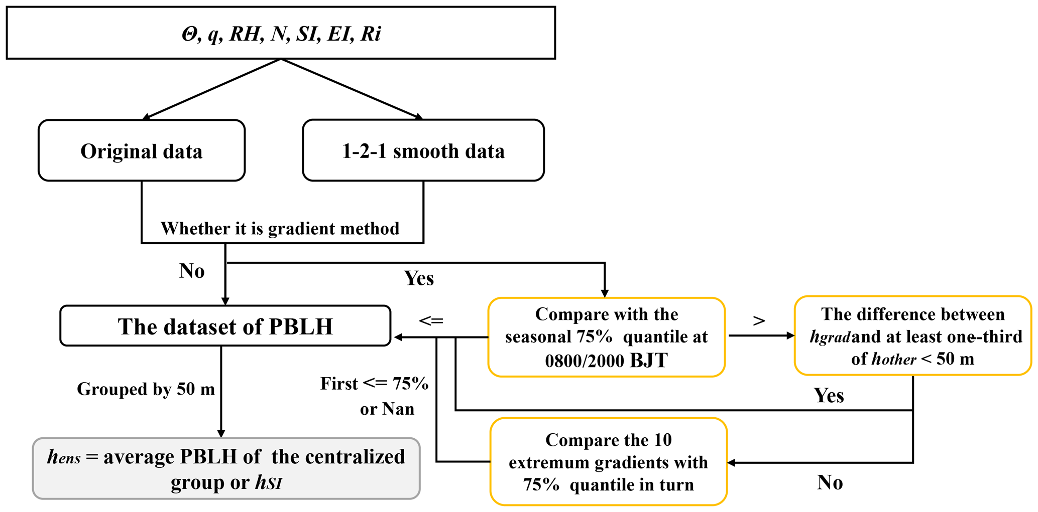
As the PBLH values derived from existing methods show obvious disagreement and misjudgment, we proposed an ensemble method to automatically obtain a consistent estimation of PBLH in the transition. Seven methods introduced in the previous section are included in the ensemble method to make up for the shortcomings of a single approach and to make it more suitable for different types of boundary layers. For all methods, to avoid taking tropospheric features as the PBL top, we restricted the radiosonde data to 3000 m according to the long-term climatology of PBLH in China (Guo et al., 2019, 2021). To avoid noisy readings near the surface (Liu and Liang, 2010), we only consider the stable boundary layer higher than 100 m a.g.l. Besides original data, three-point smoothing was also introduced to eliminate the fluctuations in high-resolution data, and more details are illustrated in the Supplement. Based on these constraints, the procedures of our ensemble method are specifically described as follows:

• 1.

  Apply the seven individual methods to both the raw data and the smoothed data, respectively, which are illustrated in Fig. 1. Notice that the EI method will only be implemented when the result of the SI method is null.

• 2.

  Modify the results of gradient methods (θ, RH, q, and N). Get the 75 % quantiles of initial results of gradient methods from the observations at 08:00 and 20:00 BJT for each season, respectively. Compare the result of each gradient method with the corresponding 75 % quantile. If the initial result is greater than the corresponding 75 % quantile, then get the difference between the result and other methods. Accept the result if at least one-third of differences are less than 50 m. Otherwise, go through altitudes of the 10 smallest (or largest for θ) gradients and replace the initial result with the first altitude less than the 75 % quantile. If all altitudes do not meet the criteria, then the PBLH for the specific observation is null.

• 3.

  Group the PBLH data set after modification by 50 m. Determine the average of the group with the largest data volume as the ensemble PBLH (h_ens). If the result of the SI method is included in this group, then take it as h_ens.

Figure 1 The flowchart of the ensemble method.

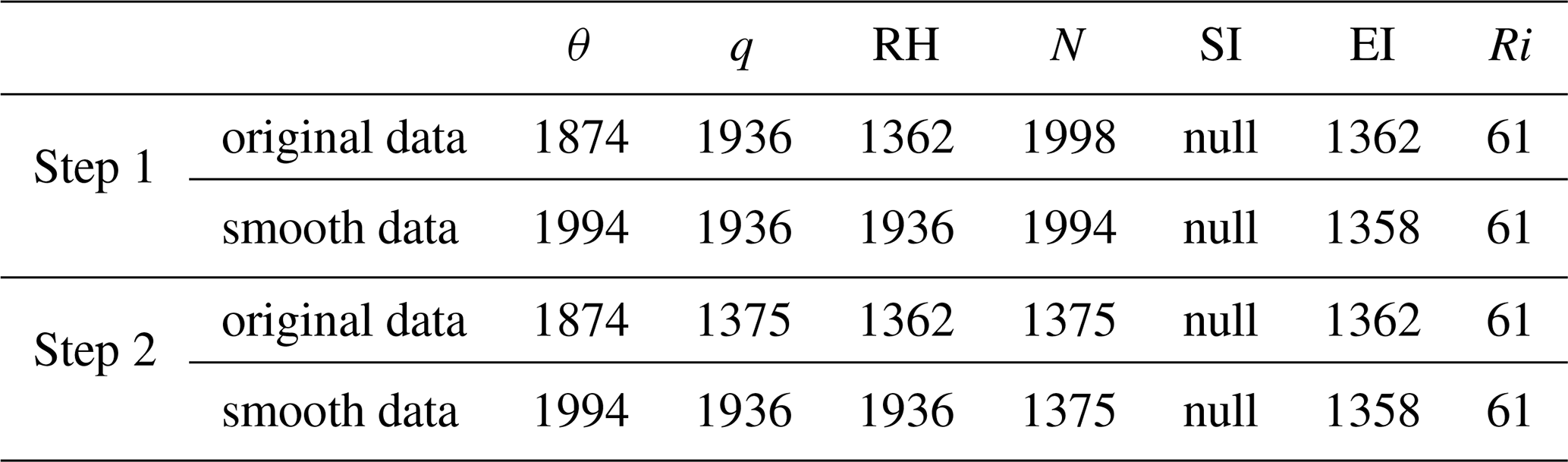
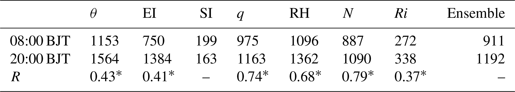
The result of each step at the specific observation time (08:00 BJT on 15 January 2017) is illustrated as follows for further explanation. The original results of seven individual methods at step 1 are presented in Table 1. As the potential temperature (θ), specific humidity (q), relative humidity (RH), and refractivity (N) methods can be thought of as gradient methods, statistical modification was carried out. As this case was observed at 08:00 BJT, the results were compared with the 75 % quantiles of each method at 08:00 BJT, which were calculated based on the whole year of observation. Here, the 75 % quantiles of each method are 1944, 1473, 1824, and 1346 m for the original data and 1959, 1599, 2110, and 1516 m for the smoothed data, respectively. The PBLH calculated from the original data by q method is greater than the corresponding 75 % quantile, and only two of other methods differ from 1936 m within 50 m. Therefore, we went through the altitudes of the 10 largest gradients and replaced the result by the first altitude smaller than the 75 % quantile. The altitude (1375 m) of the third gradient met this criterion, and 1936 m was replaced by it. The other PBLHs that meet the same conditions were also replaced.

Table 1 The PBLHs (m) determined by seven methods in steps 1 and 2 at 08:00 BJT on 15 January 2017.

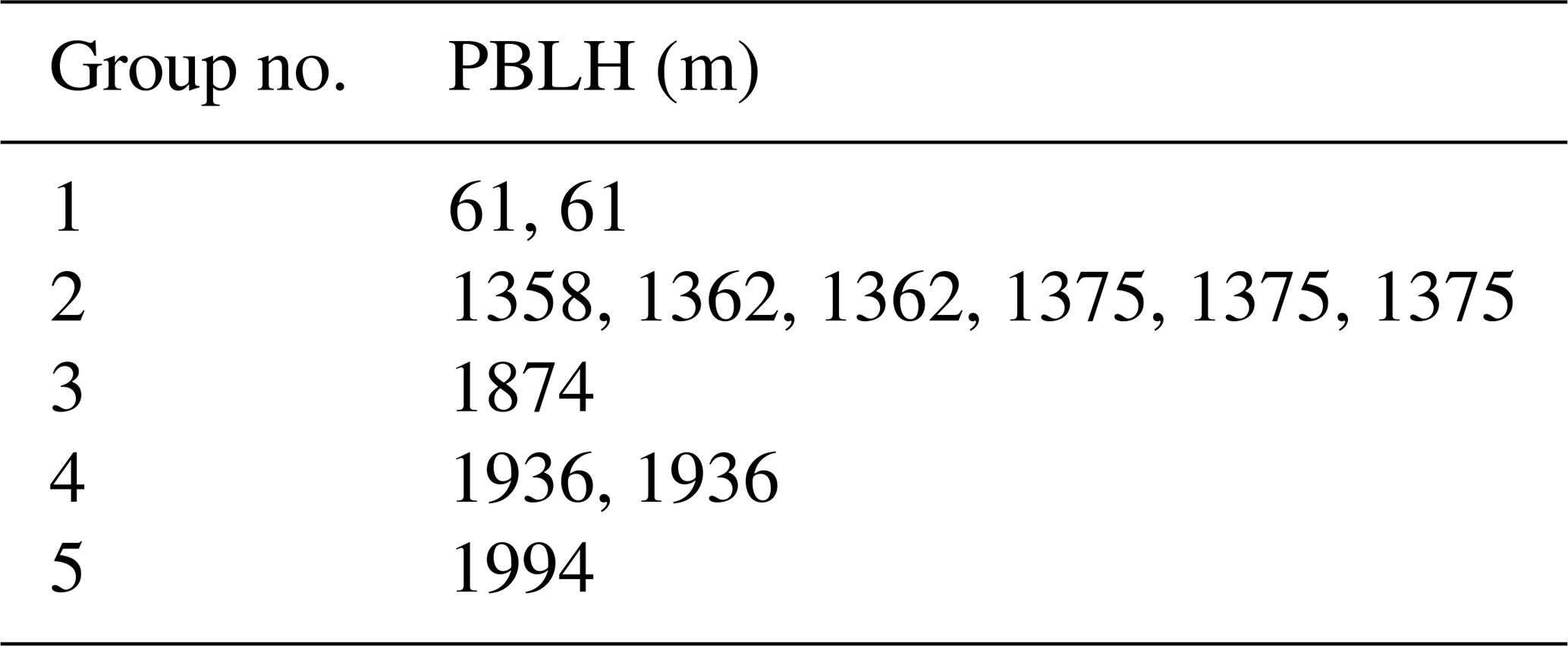
Finally, the data set in step 2 was grouped by 50 m, and the groups are shown in Table 2. As Group 2 has the maximum data volume, the average of Group 2, 1368 m, was taken as the ensemble PBLH in this case. If the result from the SI method is included in the most centralized group under other circumstances, the result from the SI method will be taken as the ensemble PBLH.

Table 2 The PBLH (m) groups in step 3 at 08:00 BJT on 15 January 2017.

2.4 Classification of PBL regimes

The CBL, stable boundary layer (SBL), and residual layer (RL) are three major regimes of the PBL in view of its thermodynamic condition (Stull, 1988; Zhang et al., 2018). The CBL usually occurs in the daytime, and the SBL occurs during nighttime because of the dominance of outgoing longwave radiation emitting from the ground surface. During the transition stage between CBL and SBL, the PBL structure can be complex, including the neutral RL that started from the ground surface with no evident CBL or SBL (Fig. 2b), a weak convective layer, and a weak stable layer with RL located at the top. Herein, we define the above-mentioned PBL regimes as a transition stage (TS). The criteria of classifying the PBL regimes by examining the near-surface thermal gradient refer to Liu and Liang (2010), and some parameters were modified according to the actual application. Figure 2 illustrates three real atmosphere cases for each PBL regime. The potential temperature difference (Δθ) between level k (the first level right above 100 m ground level) and level 2 (the second received data) was applied as the diagnostic quantity. Through visual validation, the limit of Δθ is −0.2k for CBL and 1k for SBL; all other cases are classified as a TS.

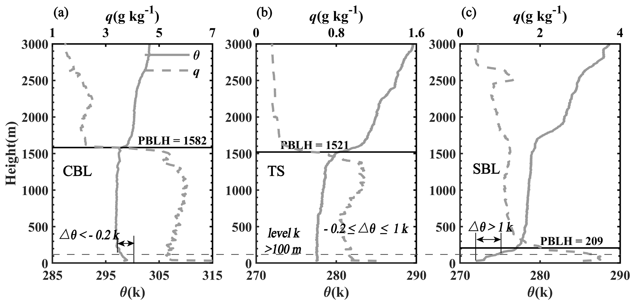
Figure 2 The PBL structure from cases (a) at 14:00 BJT on 3 June 2017 for CBL, (b) at 08:00 BJT on 12 March 2017 for the TS, and (c) at 20:00 BJT on 8 January 2017 for SBL, respectively. The procedure of PBL classification is illustrated by the annotation ($\mathrm{\Delta }\mathit{\theta }={\mathit{\theta }}_k-{\mathit{\theta }}_{\mathrm{2}}$).

3 Results

3.1 Valid cases under different conditions

The effectiveness of the ensemble method is first visually illustrated by several cases under different conditions. To assist the verification, the range-squared-corrected signal (RSCS) at 1064 nm from a ground-based lidar located at the Institute of Atmospheric Physics (IAP), Chinese Academy of Sciences (CAS) (39.982^∘ N, 116.385^∘ E), is shown along with the radiosonde profiles. More information about the ground-based lidar can be found in Wang et al. (2020). The PBLHs determined by the widely used gradient method (GM), which takes the position of the minimum gradient of RSCS as the PBLH (Flamant et al., 1997), are also marked on the lidar signal profiles.

3.1.1 A case in the afternoon

Since the PBLH definition for the CBL is relatively clear and previous integrated methods are mainly concerned with this condition, our ensemble method was first evaluated when a CBL occurred to prove the reliability preliminarily. The observations in summer were intensified for improving the accuracy of severe weather forecasting, resulting in additional sounding at 14:00 BJT, which usually corresponds to vigorous CBL. Thus, a case at 14:00 BJT on 7 June (Fig. 3) was chosen. As illustrated in Fig. 3a, different gradient methods initially determined the PBLH from 2455 to 2590 m, and these results exceeded the corresponding 75 % quantile. Among the results from original data and smoothed data, the consistent results (difference <50 m) accounted for less than a third of the total, and that triggered the statistical modification of overestimation from gradient-based methods. From Fig. 3b, we can see that the PBLH is about 2200 m at 13:00 BJT and eventually decreased to about 1500 m at 15:00 BJT. Therefore, a sudden decrease of PBLH from 2500 to 1500 m in 1 h is obviously unreasonable. After the modification of gradient-based methods, the ensemble method finally determined the PBLH at 1965 m, which is 300 m less than the PBLH retrieved by GM. The boundary layer developments between these two sites are not completely synchronous due to the distance of dozens of kilometers. Hence, we affirmed the result of the ensemble method is valid, and the elimination of abnormally high PBLH in step 2 works.

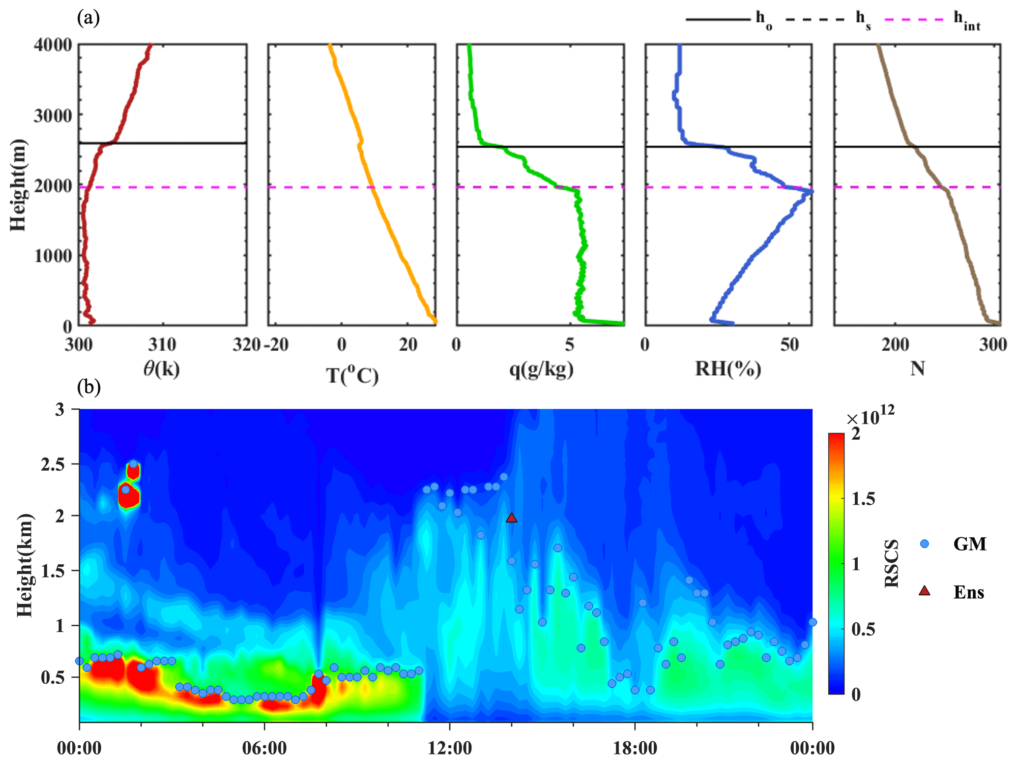
Figure 3 (a) The profiles of potential temperature (θ), temperature (T), specific humidity (q), relative humidity (RH), and refractivity (N) at 14:00 BJT on 7 June 2017. h_o is the PBLH determined by original data, h_s is the PBLH determined by data with three-point smoothing, and h_ens is the PBLH determined by the ensemble method. (b) Evolution of the lidar RSCS signal at 1064 nm on 14 June 2017. The PBLHs retrieved from gradient method (GM) are marked by blue dots, and the h_ens in panel (a) is marked by a red triangle.

3.1.2 A case study during the morning transition period

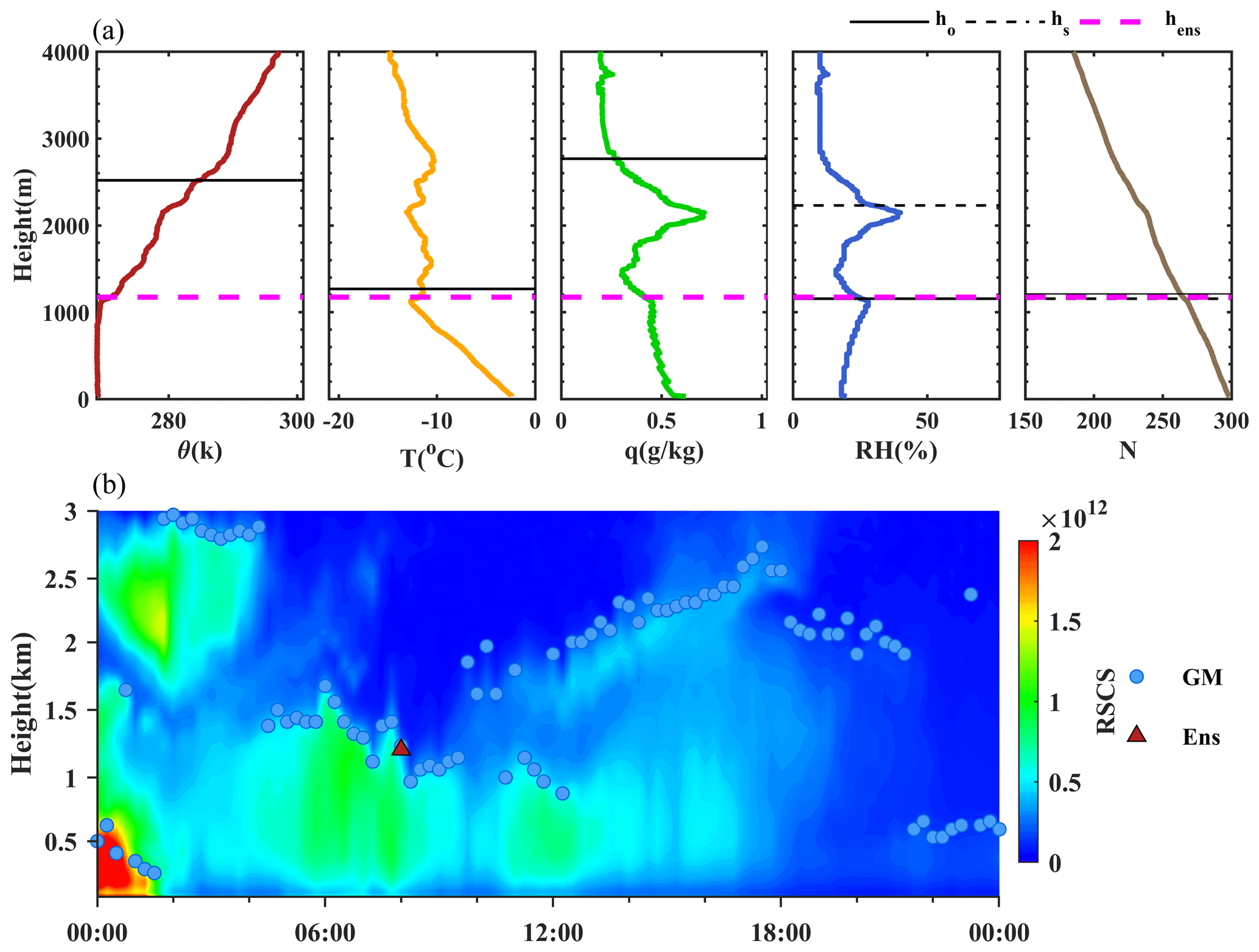
During the morning TS, the top of the RL continues to collapse with the infrared radiative cooling overnight. On the other hand, the CBL started to grow after sunrise. A case on 29 January with a distinct RL collapse process is shown in Fig. 4b. We can clearly identify from the lidar RSCS signal profile that the PBLH decreased from approximately 1500 to 900 m in the early morning, and it is 1230 m at 08:00 BJT. According to the radiosonde profiles, there is no superadiabatic or inversion layer near the surface, and this case can be classified as a neutral RL. Different from the consistent overestimation in Fig. 3, the PBLHs of each method vary greatly from 1156 to 2768 m, among which the q method is the highest and the RH method is the lowest. This kind of divergence usually requires manual verification to determine the final PBLH. However, with the clustering in the ensemble method, the outlier results from θ, q, and RH methods were automatically eliminated. The PBLH was determined at 1175 m, and it shows a good consistency with the continuous boundary layer collapse from the lidar signal profile.

Figure 4 Same as Fig. 3 but (a) at 08:00 BJT on 29 January 2017 and (b) on 29 January 2017.

3.1.3 A case study during the evening transition period

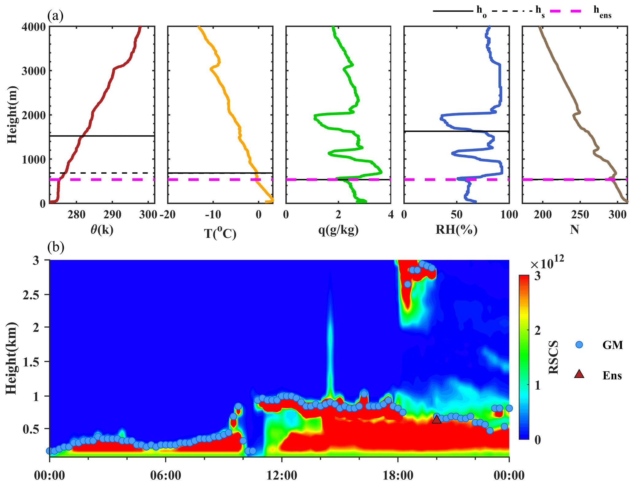
Compared to the morning transition, the evening transition period can be longer. Figure 5 presents a case during an evening transition period with a multi-layer structure to illustrate the applicability of the ensemble method in a complex boundary layer structure. According to the satellite cloud product and the humidity profiles of radiosonde, there were multi-layer clouds on 5 January. The complex temperature and humidity profile caused the misestimation of PBLH at approximately 1600 m by θ and RH methods. The air quality was poor, and the aerosols gathered below PBLH on that day. In this case, the lidar RSCS signal profile shows the position of PBLH well. Constrained by the clouds, the warming effect of solar radiation after sunrise was weaker than the previous two cases, and the maximum PBLH developed to 1000 m at 12:00 BJT. On the other hand, the presence of clouds also slowed down the radiative cooling at night, and the PBLH decreased slowly from 900 m (17:30 BJT) to 600 m (20:00 BJT) after sunset. Obviously, the PBLH over 1000 m from θ and RH methods during evening transition is not consistent with the evolution of PBL. The ensemble method excluded the outliers of the PBLH and determined the PBLH at 536 m, which is close to the inversion results from lidar.

Figure 5 Same as Fig. 3 but (a) at 20:00 BJT on 5 January 2017 and (b) on 5 January 2017.

3.2 Effectiveness and uncertainty of the ensemble method

Several cases discussed above have already shown that the ensemble method is effective. In this section, we will further prove the effectiveness and reliability of the ensemble method by statistical approaches. First, we compared the statistical characteristics with the existing methods. Table 3 shows the average PBLHs determined by seven existing methods and the ensemble method at two routine observation times. Note that all PBLHs estimated by individual methods are derived from original data in the statistical analysis. The average values of PBLH are between 150 and 1600 m. The PBLHs at 08:00 BJT are consistently lower than those at 20:00 BJT except for the SI method, as longer surface-radiation cooling contributes to the further development of SBL. The average PBLH from the ensemble method is 911 and 1192 m at two routine launch times, respectively. Comparing the other methods, we found the θ method yields a consistently higher PBLH, and the results are more discrete (Fig. S3 in the Supplement). The PBLHs based on the RH gradient are also consistently high, and that may be explained by the sensitivity of RH profiles to cloud-top heights (Seidel et al., 2010). The q method shows good consistency with the ensemble method at 20:00 BJT with an average of 1163 m PBLH. However, the N gradient method gave closer average PBLHs to the ensemble method at 20:00 BJT, with the highest correlation coefficient of 0.79. Moreover, the PBLHs derived from the Ri method were systematically underestimated with an average of about 300 m, which is comparable with the average nighttime PBLH in China (Guo et al., 2016a). The average PBLHs and correlation analysis with existing methods preliminarily show the rationality of the ensemble method. Meanwhile, the drawbacks of different methods are also on display.

Table 3 The average PBLHs (m) determined by eight methods at two routine observation times and the correlation coefficient (R) of individual methods with the ensemble method.

^* Data passed the significance test.

To further illustrate the effectiveness of the ensemble method, the PBLH results of each case were verified manually with the aid of lidar observation. If the error between the result of the corresponding method and the truth PBLH value is within 50 m, then the result will be considered valid. Therefore, the effectiveness of each method is defined as follows:

$$\begin{array}{}\text{(3)}& E={\displaystyle \frac{\text{number of valid samples}}{\text{number of all samples}}}\times \mathrm{100}\mathit{\%}.\end{array}$$

We measured the E of each method over a year of observations, and the results of existing methods are still derived from original data. The Ri method shows the lowest E of 9.6 %, and this can also be inferred from the underestimated PBLH in Table 3. As SI and EI method only be executed under specific conditions, E_SI and E_EI are also low. Among four gradient methods, E_θ is 33.9 % and the others have a higher E. They are 51.2 %, 48.0 %, and 56.1 % for the q, RH, and N methods, respectively. Compared to these methods, E_ens (62.6 %) has been significantly improved.

Despite the good performance of the ensemble method, there are still some uncertainties in the calculation process. The upper quartile was chosen as the threshold in step 2 as it is widely used in statistics to get a reasonable data range. We also suggest to get the climatology value from the previous research on the climatology of PBLH for practical application. Apparently, the different thresholds could derive different PBLHs. To illustrate the uncertainty of PBLHs discussed in this paper, we compared the average PBLHs of different PBL regimes using 70 %, 75 %, and 80 % quantiles as the threshold in step 2. The higher the threshold is, the higher the average PBLH is. The average PBLHs of all observations are 1098, 1109, and 1135 m for corresponding thresholds, and there were only about 2.9 % (24) cases in which the PBLH changed by more than 100 m. In addition, the PBL in the TS was most affected, and the SBL was least affected by the threshold. The mean PBLH of the TS increased by approximately 20 m when the threshold increased from a 70 % to a 75 % quantile and from a 75 % to an 80 % quantile. E_70 % and E_80 % are 62.3 % and 61.7 %, respectively, which means the uncertainty caused by the threshold is small. Furthermore, the number of smoothing points can be another source of uncertainty. The increase in smoothing points increased the average PBLH by about 50 m, and the difference between five-point and seven-point smoothing is small. More smoothing points may cause the loss of PBL structure, so E_7-point (57.8 %) is the lowest.

3.3 Invalid cases under different conditions

As the goal of the ensemble method is to improve the accuracy of automatic PBLH estimation as much as possible, it does not mean that there are no failures. In some conditions, the ensemble method fails. We will discuss the typical invalid cases in this section.

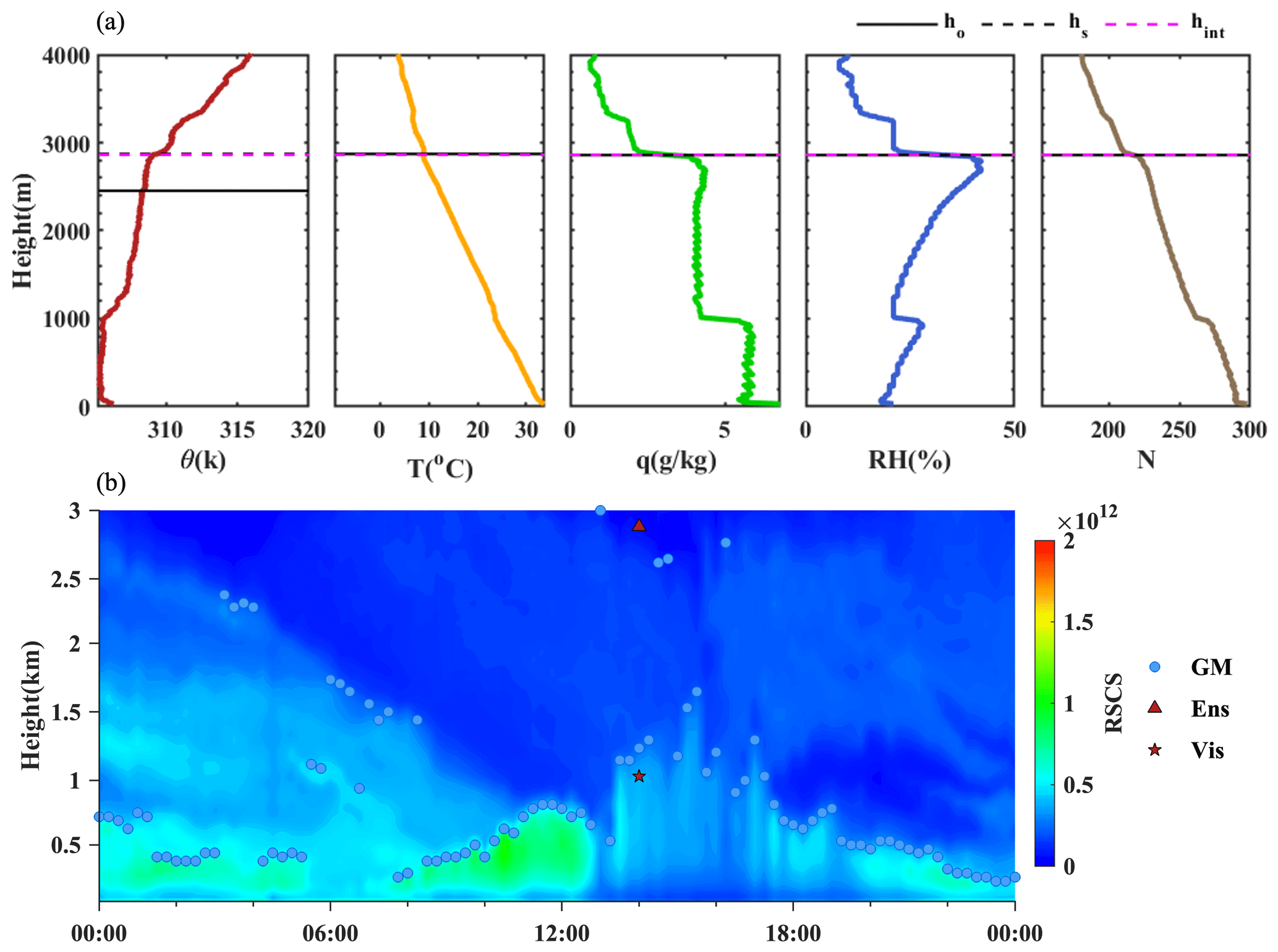
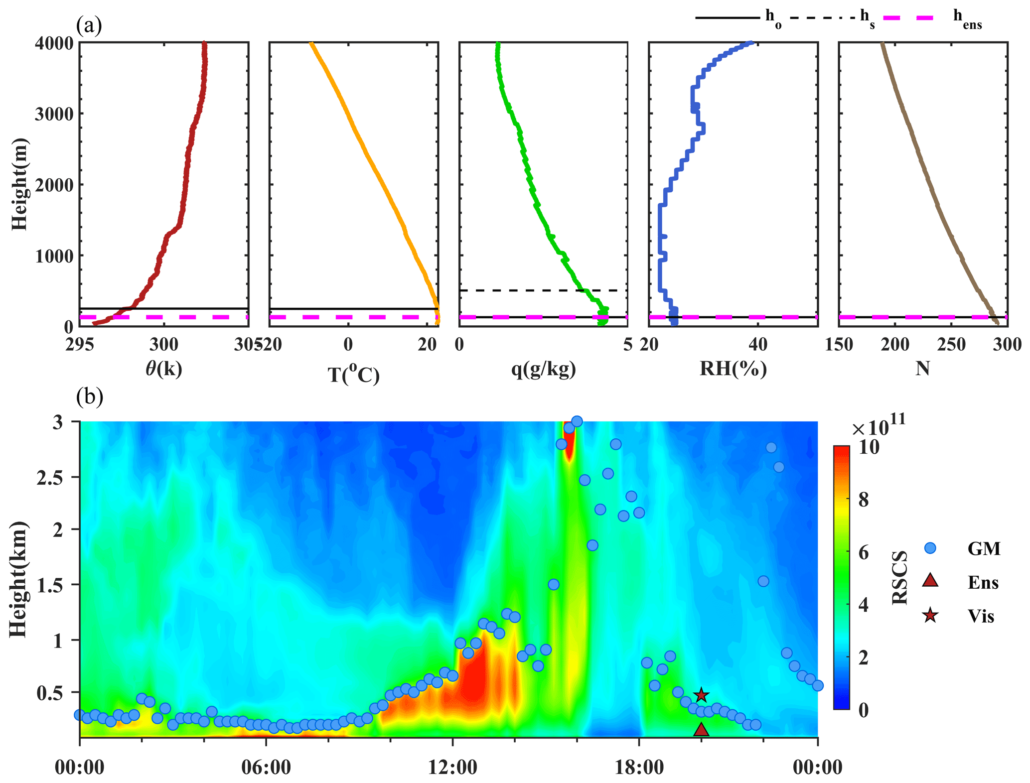
Figure 6 (a) The profiles of potential temperature (θ), temperature (T), specific humidity (q), relative humidity (RH), and refractivity (N) at 14:00 BJT on 14 June 2017. h_o is the PBLH determined by original data, h_s is the PBLH determined by data with three-point smoothing, and h_ens is the PBLH determined by the ensemble method. (b) Evolution of the lidar RSCS signal at 1064 nm on 9 February 2017. The PBLHs retrieved from gradient method (GM) are marked by blue dots, the h_ens in panel (a) is marked by a red triangle, and the PBLH of visual validation is marked by a red star.

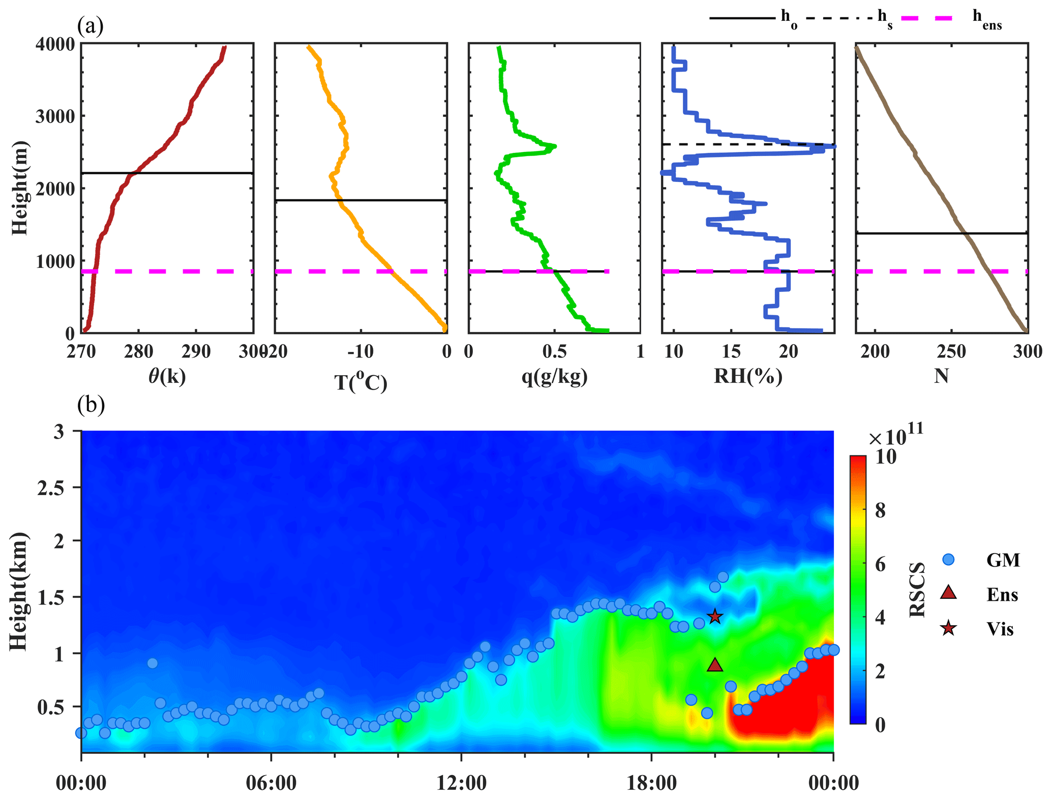
Since an internal comparison of existing methods is required before the statistical modification in step 2, the consistent overestimation of PBLH is one of the important reasons for the failure of the ensemble method. In Fig. 6, except the θ method, all methods initially determined the PBLH at 2859 m. Even though this height exceeded the 75 % quantile for q, RH, and N methods, the statistical modification was not initiated due to the consistency between different methods. There is a distinct superadiabatic layer in the profile of potential temperature, which implies the existence of CBL. The development of CBL is a continuous process promoted by the warming of solar radiation after sunrise. From Fig. 6b, we can see that the boundary layer gradually developed from 300 m at 08:00 BJT to 1650 m at 15:30 BJT. Therefore, a sudden increase of PBLH to approximately 3000 m is obviously unreasonable. The ensemble method failed in this case. Li et al. (2021) pointed out that the structure of the boundary layer will affect the reliability of the PBLH results. The ensemble method is also easy to fail when the profiles have a multi-layer structure and the divergence between different methods is substantial. A case (at 20:00 BJT on 14 January) with four moister layers in the profiles of humidity is shown in Fig. 7. The PBLHs determined by different methods were dispersed at four layers, and the scattered results led to the failure of the ensemble method to obtain the true PBLH by dominant grouping. The ensemble method mistook the first moister layer (851 m) as PBLH, while the PBLH should be 1375 m according to the continuous decline after sunset. This kind of misjudgment caused by multi-layer structure can also be seen from the lidar algorithm (Fig. 7b). Besides, the turbulence intermittency in SBL (Sun et al., 2015; Mahrt, 2014) could lead to the underestimation of SBL. Under stable conditions, the intermittency will cause discontinuous changes in meteorological elements, and Fig. 8 shows one typical case. Three gradient methods determined the PBLH at 130 m, while the inversion in the profile of temperature extends significantly higher. According to the Ri method, the PBLH at 20:00 BJT on 14 April should be 468 m and that matches the continuous PBLH evolution in lidar profiles.

Figure 7 Same as Fig. 6 but at 20:00 BJT on 14 January 2017.

Figure 8 Same as Fig. 6 but at 20:00 BJT on 14 April 2017.

3.4 PBLH of different PBL regimes

Finally, the ensemble method was applied to study the seasonal and diurnal characteristics of PBLH. According to the criteria of classifying the PBL regimes described in Sect. 2.4, the seasonal variation of the occurrence frequency of three major PBL regimes at two conventional launch times is illustrated with the average sunrise and sunset times in Fig. 9. The CBL generally occurs at 08:00 BJT in spring (20) and summer (27) when the sunrise is earlier, and the surface can become warmer with a longer period of solar radiation. Conversely, the SBL occurs more frequently in autumn and winter at both times. The occurrence of SBL in spring and summer indicates that the surface cooling can even maintain 2 h after sunrise. The TS occurred 204 and 260 times at 08:00 and 20:00 BJT, respectively. The TS occurrences are dominant in summer and spring at both times because the earlier sunrise accelerates the transition from SBL to CBL, and the sunset delayed the formation of SBL at about 20:00 BJT by surface cooling.

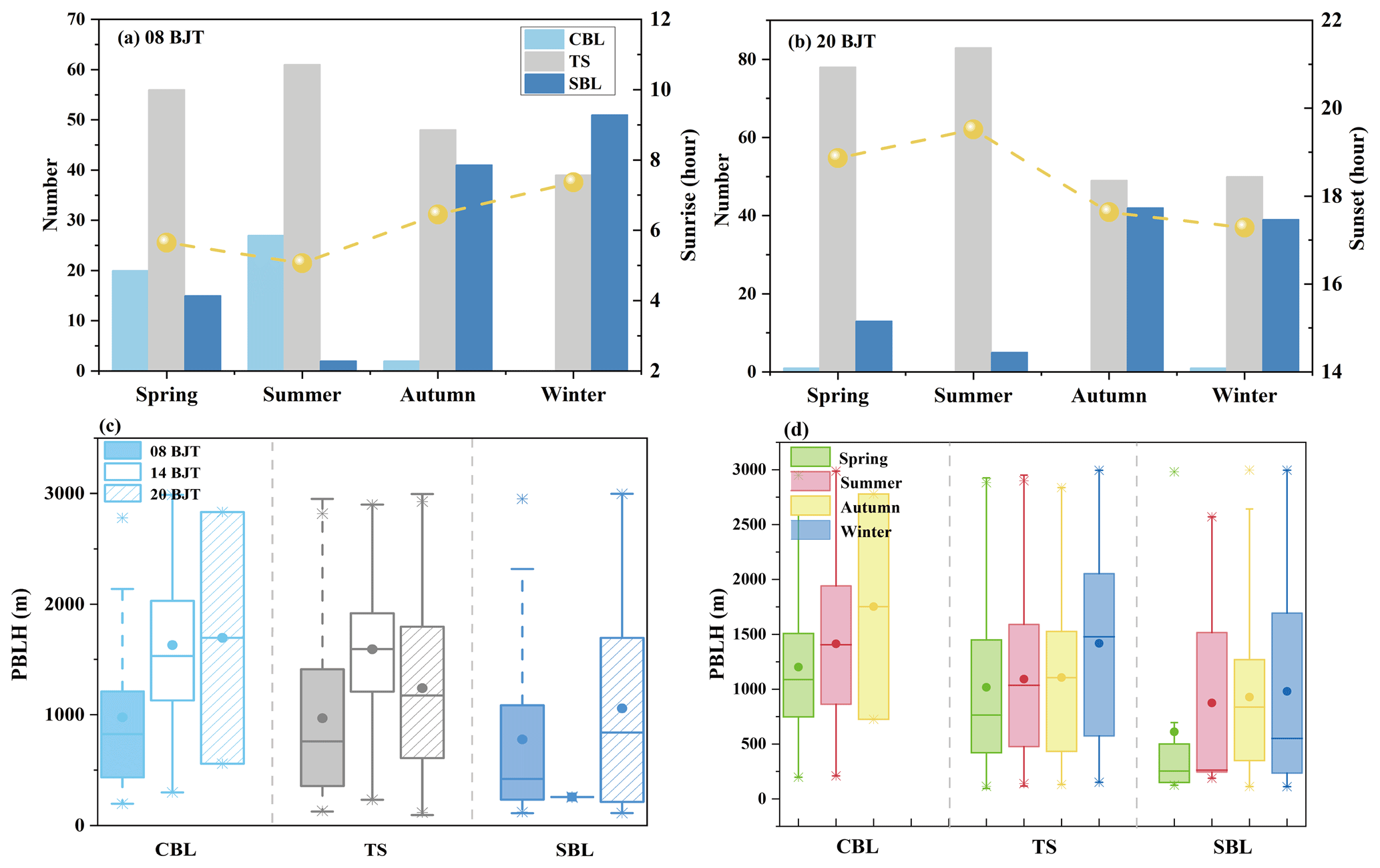
Figure 9 Histograms of occurrence number of three PBL regimes in different seasons at two routine observation times of (a) 08:00 BJT and (b) 20:00 BJT. The solid yellow circles in panels (a) and (b) represent the average time of sunrise and sunset in BJT and correspond to the right y axis. Box-and-whisker plots of three regimes of PBLs at different (c) observation times and (d) seasons (only routine observations at 08:00 and 20:00 BJT are included). The dot in each box indicates the mean value of PBLHs, and the cap represents the outlier.

The diurnal variation of PBL is preliminarily described by the observations in the morning, at midday, and in the evening (Fig. 9c). With respect to CBL, the PBLH is about 600 m higher at 14:00 than at 08:00 BJT, as the convection is most vigorous at noon. Even though the CBL could maintain after sunset, the surface cooling can attenuate the convection and make the average CBL height shrink to 727 m at 20:00 BJT. The phase peak of the TS height is also at 14:00 BJT with an average of 1318 m. Compared to the evening TS, the morning TS height falls to about 740 m after a whole night of homogenous turbulence attenuation. The mean SBL height at 08:00 and 20:00 BJT is 776 and 1056 m, respectively. The existence of remaining misjudgments of TS heights as SBL heights caused the overestimation and dispersion of the SBL height at 20:00 BJT. Besides, the two instances of SBL occurred during midday (14:00 BJT), which was also observed by Liu and Liang (2010).

The seasonal variation of PBLH observed at two routine times is presented in terms of the box plot in Fig. 9d. The average CBL height is 1201 and 1413 m in spring and summer, respectively. CBL is shown to be higher in summer, as only two instances of CBL occurred in autumn. As mentioned above, longer periods of solar radiation favor the development of convection. In contrast to the CBL, the 50th percentile value of the SBL is lower in summer with about 200 m. In winter, the 50th percentile values of the SBL rise to about 500 m due to the stronger surface cooling. The SBL is more variable in winter because of the remaining inaccuracy of PBLH estimation. The TS height lies about 1100 m in spring, summer, and autumn but 1417 m in winter.

4 Conclusions and discussion

In the present study, an ensemble method used to determine the planetary boundary layer height (PBLH) from radiosonde was proposed to reduce the inconsistency between existing methods. Seven individual methods including four gradient-based methods, elevated inversion (EI) method, surface-based inversion (SI) method, and bulk Richardson number (Ri) method are combined along with the statistical modification. The ensemble method was applied to 1-year high-resolution radiosonde data. Overall, the results show that the ensemble method has a high potential to provide a reliable estimation of PBLH for the validation of other instruments, especially in the transition period.

To illustrate the effectiveness of the ensemble method, three typical cases during afternoon, morning, and evening transition periods are presented, respectively. The results confirmed that statistical modification of gradient-based methods can effectively eliminate the overestimation caused by the presence of clouds, and the inconsistency between individual methods can be reduced by clustering. More validation was demonstrated by statistical analysis. Compared to existing methods, the annual average of PBLH from the ensemble method shows the best agreement with the refractivity (N) method: 911 and 1192 m at 08:00 and 20:00 BJT, respectively. The comparable average PBLHs to existing methods also show the rationality of the ensemble method. Further visual proof of the effectiveness (E) of each method was carried out for the 1-year observations by comparison with lidar. The Ri method shows the lowest E of 9.6 %, and the N method shows the highest E of 56.1 %. The ensemble method raised E to 62.6 %, which is 6.5 %–53.0 % higher than existing methods. Although the ensemble method shows a good improvement, there still some uncertainties in the calculation process and some cases where it is not applicable. The uncertainty of the ensemble method was evaluated by adjusting the threshold of statistical modification and the number of smoothing points. The PBLH of the TS was most affected by the increase of 5 % quantile with an increase of approximately 20 m, and E_70 % and E_80 % are close to E_75 %. The increase in smoothing points increased the average PBLH by about 50 m and decreased E. Besides, three cases with the consistent overestimation of PBLH, the multi-layer structure, and the intermittent turbulence in the SBL are presented to make clear when the ensemble method is invalid. At last, the reasonable diurnal and seasonal variations derived from the ensemble method also indicate that the method is applicable for different regimes of PBL in the transition. The average CBL height is shown to be the highest in summer, and the SBL is lowest in summer. The average PBLH of the TS is about 14:00 m in winter but 1100 m in other seasons.

Generally, our method has been demonstrated to be effective. However, this method was only conducted at one typical station due to data limitations. Thus, detailed validations should be conducted at more stations in the future for further wide applications. On the other hand, some shortcomings of the existing methods may be retained in the ensemble method. With the increase of more vertical profiles of turbulence observations, our improved understanding of the physical mechanism underlying the key physical and chemical processes in the boundary layer will help develop a better method to estimate PBLH in a more realistic way.