On the polarimetric backscatter by a still or quasi-still wind turbine

Wind turbines negatively affect the performance of weather radars, especially when located in the proximity of a radar site. In March 2019, MeteoSwiss performed a measurement campaign by deploying a mobile X-band radar in Schaffhausen. It proved to be useful for mapping and characterizing the maximum power returns by three wind turbines observed using standard scanning strategies. In March 2020, the campaign was repeated using a more sophisticated scan strategy: ∼ 100 min special sessions of fixed pointing an antenna towards the nacelle of the closest wind turbine (WT) located within a range of 7766 m from the radar, interleaved every 2 h by a scanning protocol identical to that of the March 2019 campaign. Polarimetric radar signatures were derived every 64 ms using 128 radar pulses transmitted every 0.5 ms (pulse repetition frequency (PRF) = 2000 Hz). A thorough overview of the polarimetric signatures of the WT in still or quasi-still conditions has been obtained based on 30 000 polarimetric measurables acquired over 32 min on the first day of the campaign (4 March 2020). During the first 2 min with zero rotor speed, the co-polar correlation coefficient between the orthogonal polarization states, ρ_HV, was persistently equal to 1, similarly to the signature of a bright scatterer observed by a non-rotating antenna. The changes between two consecutive values of the differential reflectivity and radar reflectivity factor were either 0 dBz or ±0.5 dBz. Due to the absence of precipitation, one could assume that the standard deviation of the differential phase shift, which was as small as 3.0^∘, can be entirely attributed to the variability of the differential backscattering phase shift. There were two 10 min periods during which the rotor moved less than 1 revolution. It is worth noting that this slow movement could be associated with a change in the blade pitch angle and the nacelle orientation, which caused extreme changes in the radar reflectivity factor. For instance, two pairs of 64 ms consecutive values reached 78.5 dBz, which is the absolute maximum reached in the whole campaign (4–21 March 2020).

1 Introduction

Wind turbines can heavily affect sensitive radar applications including weather, surveillance, precision approaching and air traffic control. Furthermore, the operation of air traffic radio navigation systems like VOR (VHF omnidirectional range) can be disturbed by nearby wind turbines (Morlaas et al., 2008; Douvenot et al., 2017). In 2021 the European countries invested about EUR 41 billion in new wind farms, covering 24.6 GW of new capacity (Brindley, 2022). As large as these quantities are, they are still far off from the European goal to reach its new climate change and energy security targets. Consequently, the expected continuous and strengthened expansion of wind farms is of major concern for the weather (Norin, 2017) and aviation radar community (Cuadra et al., 2019). Wind turbines are large objects with a variety of movement patterns, which makes them a strong source of clutter that is difficult to filter. Several studies exist in the literature regarding the impact of wind turbines on radar systems. From a weather radar viewpoint, of particular interest are those studies that discuss the issue of contamination of weather radar data (Hood et al., 2010; Angulo et al., 2015; Lepetit et al., 2019); for other sectors, the identification of adverse effects of wind turbines on the performance of air surveillance and marine radars is of great concern (Angulo et al., 2014; Cuadra et al., 2019). In general, the radar reflectivity factor of wind turbine clutter depends on various parameters such as wind turbine dimensions, incidence angle of the radiation, rotor speed, blade pitch angles, nacelle orientation and radiation frequency (Gallardo-Hernando et al., 2011; Norin, 2015; Lainer et al., 2021). In the literature, several papers about the radar reflectivity factor (and equivalent backscattering radar cross section) of the wind turbines can be found. One can separate the studies according to those dealing primarily with measurements (Bredemeyer et al., 2019; Kong et al., 2011; Kent et al., 2008) and those others using numerical investigations of virtual wind turbine models (Muñoz-Ferreras et al., 2016; de la Vega et al., 2016).

Published research dealing with other polarimetric signatures of the WT is rare (e.g., Hall et al., 2017). In a recent (4–21 March 2020), unique stare-mode campaign held in Schaffhausen (Lainer et al., 2021), the WT was continuously illuminated by a fixed-pointing antenna. As emphasized by reviewer 1 (Anonymous referee, 2020), “the measurements as they are described provide further information on the properties of other polarimetric variables at the WT location. This information is urgently needed to comprehend the WT problem, and I want to encourage the authors to add further publications based on this experiment”. This preliminary study represents a small step in the direction of filling such a polarimetric gap. However, it is important to point out that our main objective is an investigation of the dual-polarization backscattered signals by a wind turbine (WT) when its rotor speed is very small or even close to zero, as well as during the transition from zero rotor speed to the ordinary moving conditions.

The reason is connected to the emerging interest in bright scatterers (BSs) (Rinehart, 1978) as an additional tool for monitoring modern dual-polarization weather radars (Gabella, 2018). Thanks to the increased number of dual-polarization radars and the increased computational power for modeling and statistical analysis, a novel point of view regarding ground clutter has emerged. It is no longer considered to be exclusively a disturbance that needs to be rejected; rather, its spatio-temporal properties are statistically characterized in order to be used for monitoring radar hardware. This is the case of the BS, which is a tall target that is close to the radar and is hit by the antenna beam axis. It has been recently shown that the historical polarimetric and spectral signatures of a BS in Switzerland represent a benchmark for an in-depth comparison after hardware replacements (Gabella, 2021). However, since it is illuminated according to a scan strategy which is optimized for an operational monitoring of the weather (Germann et al., 2022), the typical return period for BS observations is as large as 5 min (300 s). Thanks to the recent unique MeteoSwiss stare-mode campaign in Schaffhausen (4–21 March 2020), the WT is continuously illuminated by a fixed-pointing antenna with a large number of pulses (N = 128). Using a PRF (pulse repetition frequency) as large as 2000 Hz, dual-polarization signatures are available every 64 ms (128 $/$ 2000). The fixed-pointing antenna turns out to be an important advantage if one aims to characterize the intrinsic spectral signatures of the large, bright target.

A description of the radar with the dedicated scan strategy, the geographical area of operation and the observed WT is given in Sect. 2.1. Section 2.2 presents the WT metadata, which are unfortunately available only every 600 s. Section 3 represents the core of this paper: Sect. 3.1 shows that the co-polar coefficient of a still WT (rotor speed equal to 0) is perfectly stable and equal to 1, the dispersion of both the differential phase shift and the differential reflectivity is small, and the values of the radar reflectivity factor for both polarizations also show very small variability. However, Sect. 3.2 shows that the situation becomes completely different when even a small rotation (and/or change in the blade pitch angle or nacelle orientation) takes place. Section 3.3 deals with stationary rotations for most of the 10 min; it shows that, with 64 ms sampling time (128 pulses), the maxima of constructive and destructive interferences are not observed during such ordinary moving conditions but are rather observed during the small, partial, discontinuous rotation that took place in the successive 10 min (Sect. 3.4 – a partial rotation of 216^∘). A thorough discussion is presented in Sect. 4; conclusions and the outlook are found in Sect. 5.

2 Brief description of the experimental area, instrumentation and high-temporal-resolution data

2.1 The radar site (good visibility of the wind turbine), observation geometry and scan strategy

A dual-polarization, Doppler, mobile X-band radar has been used for the measurement campaign. Some key specifications of the radar system are listed in Table 2 of Lainer et al. (2021). The radar was installed near the city of Schaffhausen (approximate coordinates: 47.700^∘ latitude and 8.664^∘ longitude using the WGS84 datum) at an altitude of 455 m. The three wind turbines of the small wind park located north of Schaffhausen are installed on a hill surrounded by forests. For the specifications and other properties (including geometry) of the wind turbines, the reader may refer to Table 1 in Lainer et al. (2021). For the whole campaign in 2020, we observed only the wind turbine with the best visibility and the maximum radar reflectivity factor observed during the 2019 campaign. This turbine was indicated as WT1 in Lainer et al. (2021); hereafter, it will be simply labeled as WT. The horizontal distance from its mast and the radar site is 7.76 km. By analyzing the output of the simulations by the X-band Ground Echo Clutter Simulator (GECS-X) described by Gabella et al. (2008), which has been run using a digital elevation model (DEM) with 50 m resolution, the radar visibility towards the wind turbines could be determined. The used approach follows the simple but effective geometric optics assumption described in Gabella and Perona (1998). From the visibility map (see Fig. 1a in Lainer et al., 2021), one gets the minimum angle of elevation at which a target could be seen from the radar site, which is 2.25^∘. If no obstacles were present on the surface, then the base of the WT at ∼ 765 m would be visible from the radar site: the nominal angle of elevation using simple trigonometry (and a flat Earth) turns out to be, in fact, 2.305^∘ (see Fig. 1c in Lainer et al., 2021, but at the exact range of 7766 m of the present WT). A wood of conifers is instead present between the radar and the WT: those tall trees, at approximately 1 km range, partially block just a small part of the main lobe towards the base of the mast; on the contrary, the rotor center of the WT is always visible: knowing the nacelle height, in fact, it is easy to derive that the angle of elevation of the rotor center is 3.308^∘ (range is ∼ 7773 m). Finally, the angle of elevation for the vertical-pointing end of a blade is 3.789^∘ (range is ∼ 7777 m).

For the distinctive stare-mode strategy of the March 2020 campaign, we have opted for an angle of elevation of 3.1^∘: consequently, the whole half-power beam width (HPBW, from 2.45 to 3.75^∘, in the elevation plane) is practically not subject to occultation by obstacles. The azimuth was set to 338.9^∘. In this study, we will present polarimetric signatures derived using I and Q data of Gate103 (starting from 0), which range from 7725 to 7800 m. At such a range, the size of the pencil beam HPBW is about 180 m. On the contrary, the range resolution is independent of the range: being known a priori at what range the (weather) target should be detected and investigated, it can be pushed down to half the pulse width multiplied by the speed of light. This is, in fact, the case for our X-band radar with a pulse width of 500 ns (specifications and more details regarding the radar can be found in Table 2 of Lainer et al., 2021). It is then clear that the WT target is thoroughly bounded inside the radar sampling volume of 180 m × 180 m × 75 m (0.0243 km³) only as long as the nacelle orientation is around 0 or 180^∘. When the orientation goes toward 90 or 270^∘, part of the 65 m blades (130 m diameter) will exceed the range resolution. It is also evident that the tall, complexly shaped WT cannot be assumed to be a point target in order to retrieve a value of radar cross section from the measured power, which is in turn converted into radar reflectivity factor using the Probert-Jones (1962) approximation (Gaussian distribution of the radiated power over the main lobe). If one pretended that the point target radar equation (see, e.g., Eq. 1 in Lainer et al., 2021) were applicable and compared it with the Probert-Jones meteorological radar equation (see, e.g., Eq. 6 in Lainer et al., 2021), then the radar cross section (RCS, expressed in dB square meters) could be derived by simply decreasing by 34.4 dB the radar reflectivity factor (expressed in dBz; see Sect. 2.3.1).

2.2 Wind turbine data and metadata collection: detailed investigation during a 40 min interval starting and ending with zero rotor speed

The focus of the present study is limited to dual-polarization backscattered signals in correspondence with a situation with zero rotor speed. Hence, the prerequisite is the presence of a 10 min interval without any rotor rotation. Despite being unusual, this situation happened on the first day of the campaign, namely between 17:00 and 17:10 UTC on 4 March 2020. We are aware of such special conditions thanks to Hegauwind GmbH & Co. KG Verenafohren, who kindly provided the operational data of the wind turbines. These include environmental (e.g., wind speed, direction, outside temperature), instrumental (indoor and hardware temperature, current, voltage, power) and operational (e.g., nacelle direction, rotor speed, pitch angle of the three blades) data for a total of almost 100 parameters. Unfortunately, such an abundance of parameters cannot compensate for the main limitation of these data, which is their granularity. As a matter of fact, they are available only every 10 min, while the high-temporal-resolution radar echoes are available every 64 ms. As shown by Lainer et al. (2021), the average rotor speed and the blade pitch angle are by far the most important information for radar-related studies. For instance, zero (or very small) rotor speed is typically associated with a large value in terms of the angle of the three blades, as can be seen in Fig. 1 (red vs. blue dots).

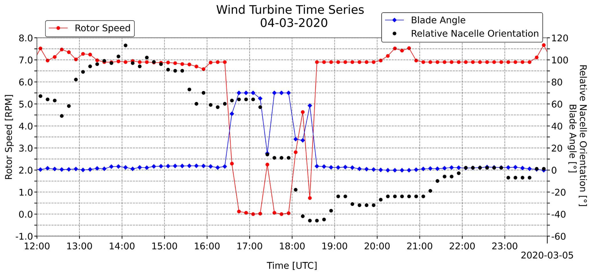
Figure 1 Wind turbine rotor speed (red, left y axis), blade pitch angle (blue, right y axis) and nacelle orientation (black dots, right y axis) on 4 March 2020.

During the first 12 h of the campaign (4 March 2020), the 10 min average rotor speed was particularly large (not shown), ranging from 7 to 11 rpm (being an energy production period, blade pitch angle was close to 0). In the second half of the day, which is displayed in Fig. 1, a 4 h period with an almost constant rotor speed (∼ 7–8 rpm) took place, followed by a quiet period between 16:40 and 17:00 UTC (average rotor speed around 0.1 rpm – red dots; blade pitch angle at 70^∘ – blue dots). In particular, the conditions during the 17:00–17:10 UTC interval on 4 March 2020 were ideal from our viewpoint: the average rotor speed was exactly 0 rpm, and so we know no movements happened (the blade pitch angles were also kept constant at 70^∘). During the (final) 2 min with available radar data (period P1; see Figs. 2–5), we will see that radar measurables are very stable with no (or very little) variability. This fact will be investigated at the original very high temporal resolution of 64 ms and displayed using a re-sampled 8 s temporal resolution in Sect. 3.1. The (8 s) low-resolution analysis is based on the maximum, minimum and median values of 125 original (64 ms) echoes. The nacelle orientation with respect to the radar beam axis was about 61^∘ (see Fig. 3a, Lainer et al., 2021; an orientation of 0^∘ means that the nacelle is pointing towards the radar).

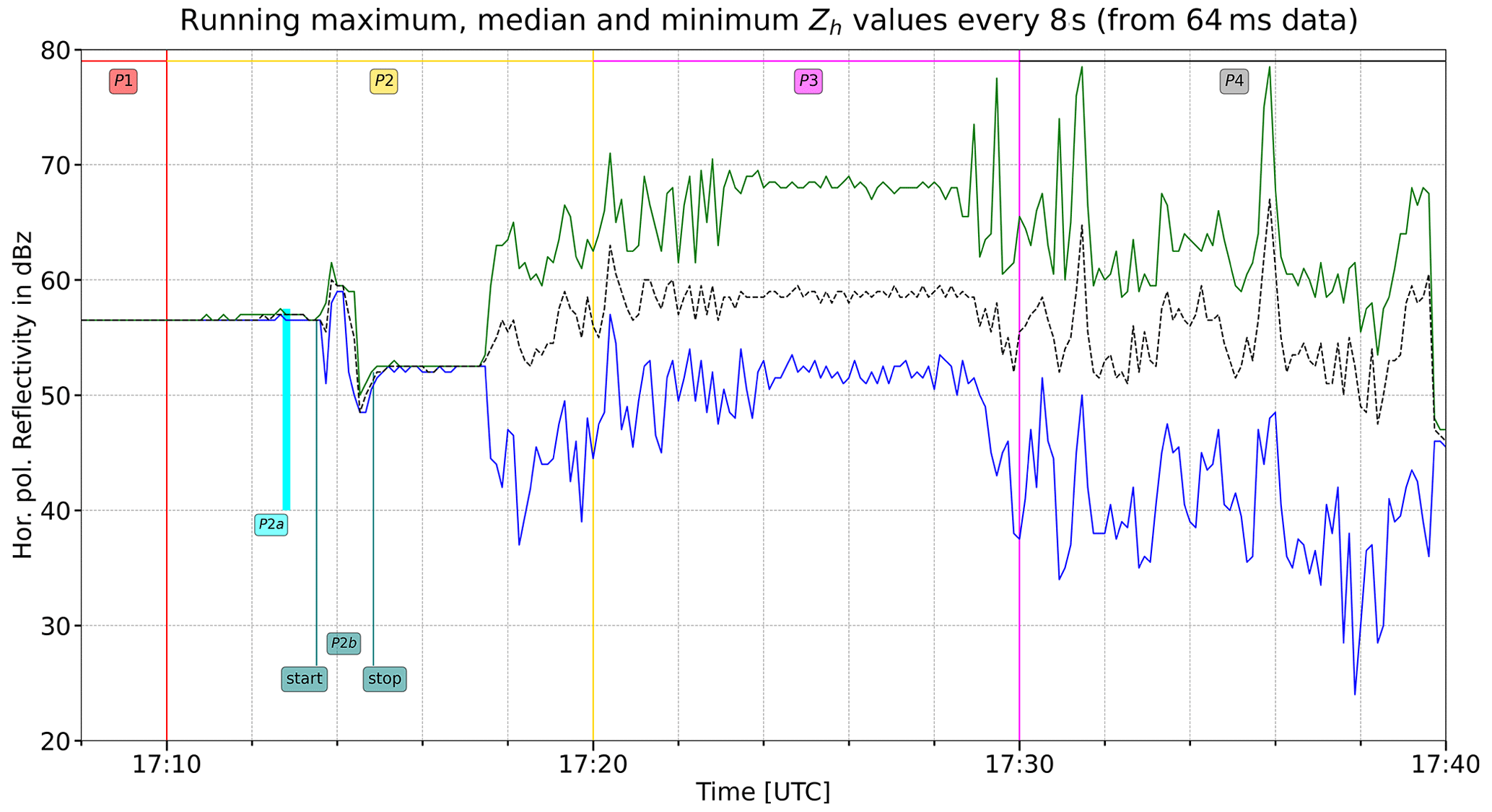
Figure 2 Time line plot of horizontal polarization reflectivity for the 75 m radar gate that contains the wind turbine. The solid lines join 8 s statistical values (median using black, maximum using green, minimum using blue) obtained by using 125 consecutive radar echoes at the original 64 ms resolution. Being the visualization based on 8 s points, the solid lines consist of 240 points that cover 32 min (15 points every 2 min, which is in correspondence with the vertical grid lines).

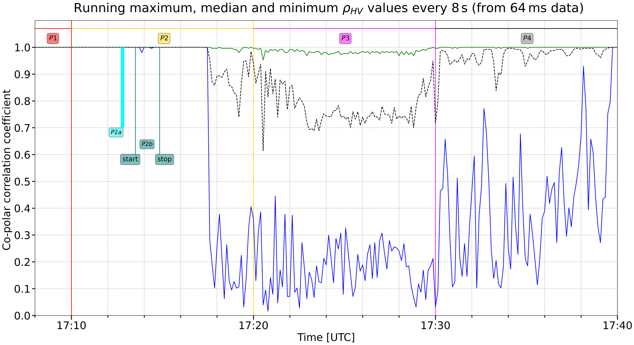
Figure 3 Same as Fig. 2 but for the co-polar correlation coefficient, ρ_HV. It is interesting to note that the zero-rotor-speed condition read from the WT metadata for the 17:00–17:10 and 17:40–17:50 UTC 10 min intervals is probably also prolonged for several minutes after 17:10 UTC, as well as being anticipated for ∼ 40 s before 17:40 UTC.

Figure 4 Same as Fig. 2 but for the vertical polarization.

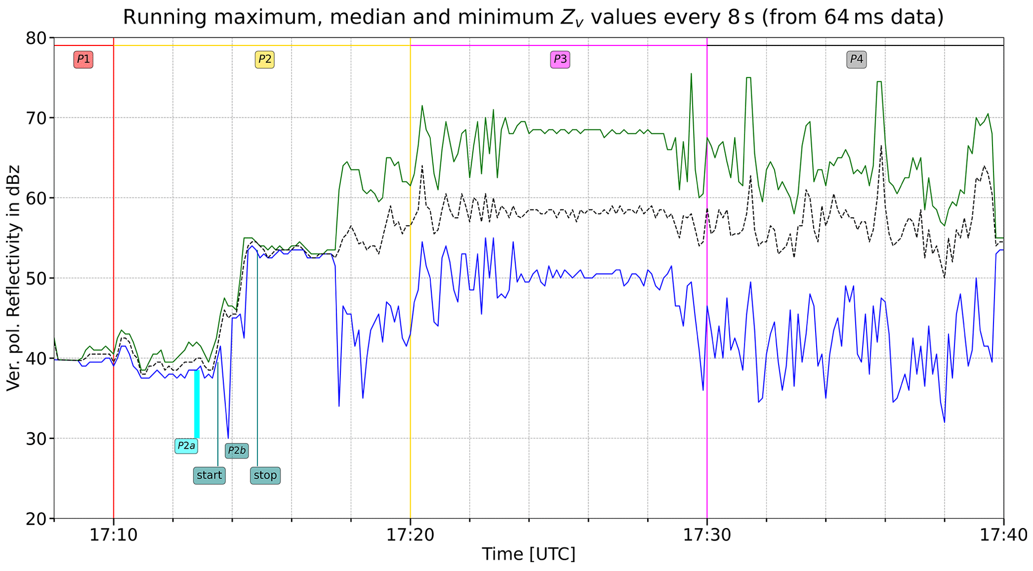
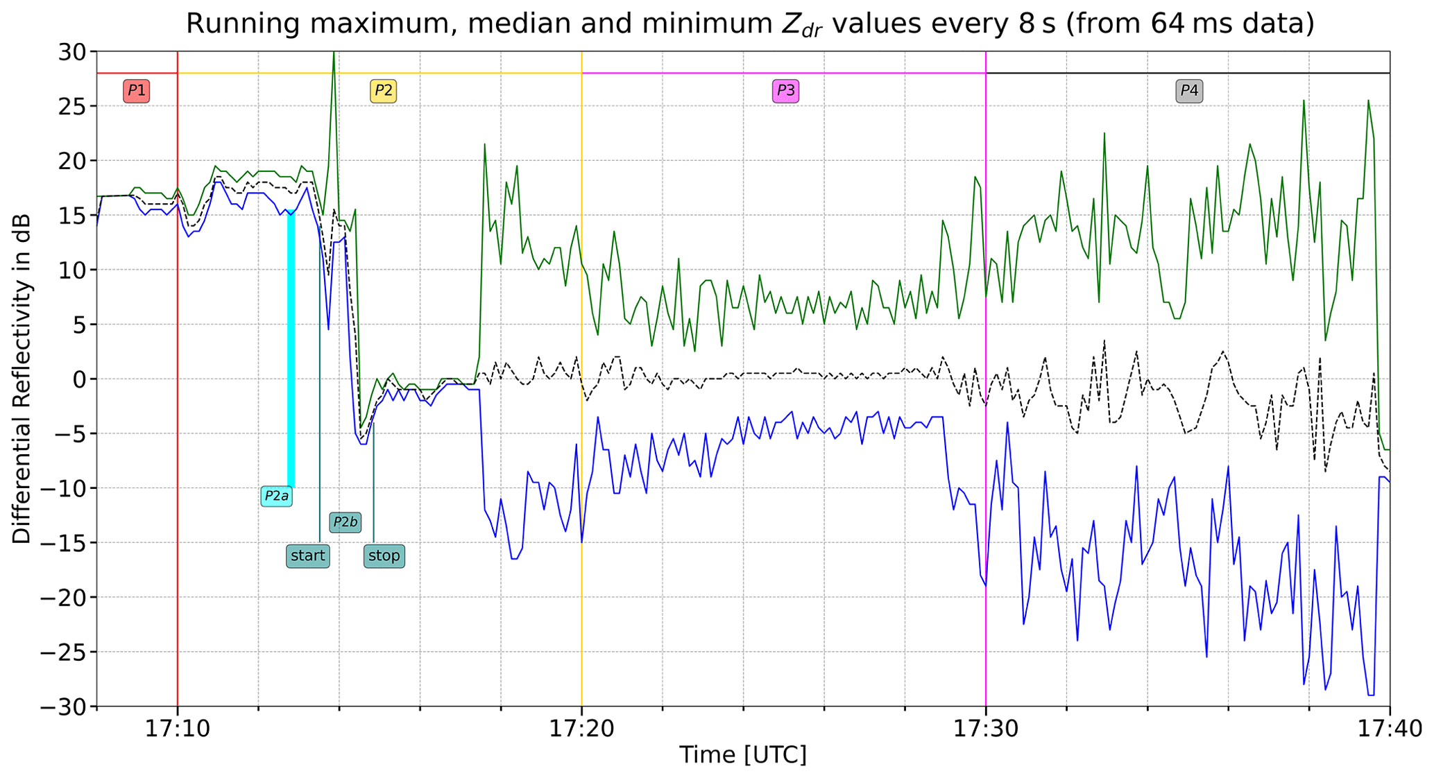
Figure 5 Same as Fig. 2 but for the dimensionless differential reflectivity. Most of the 125 echoes between 17:24:00 and 17:24:08 UTC recorded a differential reflectivity value equal to 0 dB (Z_H = Z_V). During these 8 s, Z_H (Z_V) never exceeded Z_V (Z_H) by more than 5 dB (64 ms sampling time, which means 125 echoes). Although the median (and the mode, not shown here) are, in general, around 0 dB, they are not so during the initial and final intervals characterized by zero rotor speed: our hypothesis is that, in a steady condition, the differential reflectivity depends on the position of the blades and their orientation angles.

The analyses of the successive period P2 (17:10–17:20 UTC) will be presented in Sect. 3.2. During P2, the blade pitch angles were reduced from 70 to 65^∘ (see Fig. 1, blue dots, y axis on the right), while the nacelle orientation was changed from 61 to 57^∘ (Fig. 1, black dots). The rotor was turned, probably exclusively during the last 2 min, by a 0.2 rotation, which corresponds to 72^∘.

Then, between 17:20 and 17:30 UTC, period P3, the rotor started its typical rotation, though at a speed (2.25 rpm) that was smaller than usual and with blade pitch angles that were larger than usual but still close to just a few degrees. The nacelle orientation changed significantly: from 57^∘ to just a few degrees, where it also remained during period P4 (17:30–17:40 UTC). P4 (see Sect. 3.4) was characterized by a partial rotation of 216^∘ and a different value of the blade pitch angles, which were again set to 70^∘. Interestingly, the largest RCS value at a horizontal polarization occurred twice with this configuration (see Sect. 4 for more details).

2.3 The polarimetric weather radar measurables (available every 64 ms)

2.3.1 First measurable: radar reflectivity factor at horizontal and vertical polarization

One of the most used quantities measured by weather radar is the so-called radar reflectivity factor. The backscattered received power, p_r, caused by the hydrometeors and detected by the radar is, in fact, directly proportional to the radar reflectivity factor, z (throughout the paper, we will simply use reflectivity to refer to it). Since both the received power and the reflectivity span several orders of magnitude, they are often expressed using a log-transformed scale after the division of the physical quantity by a normalization factor. For linear received power, p_r, the normalization value is typically p₀ = 1 mW. The typical normalization value for the reflectivity is z₀ = 1 mm⁶ m⁻³. The dual-polarization radar can simultaneously measure two reflectivity values associated with two orthogonal polarization planes: they will be indicated as z_h and z_v in linear units or Z_h and Z_v after the log transformation. As stated, [z_h] = [z_v] = mm⁶ m⁻³, while [Z_h] = [Z_v] = dBz. The upper case P_r indicates the log-transformed received power, where [P_r] = dBm.

As far as the quantization is concerned, a value of 0.5 dBz was chosen by the radar manufacturer. At MeteoSwiss, an identical choice was made regarding the reflectivity resolution of the five C-band radars of the Swiss network; also, the formula for converting from eight bits to a physical value is identical. The linear conversion from the 1-byte digital number (DN) to the log-transformed radar reflectivity is as follows:

$$\begin{array}{}\text{(1)}& Z_{\mathrm{dBz}}=\left(\mathrm{DN}-\mathrm{64}\right)/\mathrm{2}.\end{array}$$

However, the maximum recorded value observed operationally in Switzerland (both in the C-band network and with this mobile X-band radar) rarely exceeds 85 dBz (DN = 234); furthermore, a weak echo corresponding to DN = 14 (−25 dBz) can only be detected at a distance of 1 km or closer from the X-band radar.

2.3.2 Second measurable: differential reflectivity

The differential reflectivity, Z_dr, is an important polarimetric quantity that can be derived by combining the previously described two measurables in a differential manner: it is defined as the log-transformed ratio between the co-polar linear reflectivity measured using horizontal (z_h) and vertical (z_v) polarizations.

$$\begin{array}{}\text{(2)}& Z_{\mathrm{dr}}=\mathrm{10}\mathrm{Log}\left(z_{\mathrm{h}}/z_{\mathrm{v}}\right)\end{array}$$

The differential reflectivity is expressed in dB, and a value of 0 dB means that z_h = z_v. In practice, Z_dr can also be computed as the difference between Z_h and Z_v. The differential reflectivity was introduced by Seliga and Bringi (1976) for a better estimate of rainfall since it contributes to reducing the uncertainty associated with raindrop size distributions. Indeed, the information carried by Z_dr is valuable; however, the issue of a proper calibration remains a challenge for successful quantitative precipitation estimation. As far as the quantization is concerned, 256 values (eight bits) are linearly assigned by the manufacturer over an interval that spans 16 dB (from −8 to +8 dB). We will see in Sect. 3 that, surprisingly, many WT echoes are outside this interval. Consequently, in this study, we abandon such $\mathrm{1}/\mathrm{16}$ dB radiometric resolution and use the poorer 0.5 dB resolution that permits us to derive the value in all circumstances simply as the difference between Z_H and Z_V.

2.3.3 Third measurable: module of the co-polar correlation coefficient between horizontal and vertical polarization

An important quantity measured by dual-polarization radars is the correlation between the co-polar horizontal and vertical returns, called the co-polar correlation coefficient (often referred to as ρ_HV, sometimes as ρ_co). The co-polar correlation coefficient is connected with the differential reflectivity: it is, in fact, related to the dispersion of the differential reflectivity of the 128 instantaneous backscattered signals (with a pulse repetition time of 0.5 ms) used to derive each echo every 64 ms. For a detailed and clear description of the interesting and complicated nature of this measurable, the reader may refer to e06.1, which is the first part of the electronic supplement number six accompanying the book by Fabry (2015). Here, it is sufficient to remind ourselves that it is the module of the complex correlation coefficient between two orthogonal polarization components and that it ranges from 0 (no correlation between the two polarizations) to 1 (perfect correlation). If targets within the radar sampling volume were similar, then the time series of signals at horizontal and vertical polarizations would be highly correlated in both amplitude and phase. On the contrary, the greater the variability in the shapes of the targets, the smaller the value of ρ_HV will be. When many backscatterers are randomly distributed within the sampling volume, the co-polar correlation coefficient is considered to be a measurement of shape diversity. Consequently, the echoes of light rain and drizzle (small and similar spherical drops) are associated with very large values of ρ_HV, mostly larger than 0.995; ρ_HV values in melting snow are lower (typically between 0.8 and 0.9) and make the melting layer easily distinguishable. If the sampling volume contains a significant number of different targets, such as what happens with ground clutter, ρ_HV will decrease considerably. In particular, the range of ρ_HV for most ground clutter echoes is between 0.650 and 0.950. Since the most interesting values are very often close to 1, typically, a logarithmic function is used in the quantization process when assigning a DN to the original floating point value of ρ_HV (see, for instance, Eq. 6 in Gabella, 2018, for the MeteoSwiss quantization formula that permits increments as small as 0.0001 when close to 1). The X-band radar manufacturer has opted for a linear stretch from 0 to 1, which means equal increments of 0.0039 over the whole interval. This choice is certainly not optimal: for instance, during 5 clear-sky days, when 1440 echoes backscattered from the tower at Cimetta have been analyzed (see Sect. 3.5.1 of Gabella, 2018), the present quantization would only use four DNs (from 252 to 255, with a mode at DN = 254, which is ρ_HV = 0.9961), while MeteoSwiss quantization had DNs ranging from 180 to 251, with a mode at DN = 233, which is ρ_HV = 0.9982.

2.3.4 Fourth measurable: differential phase shift of the co-polar signal at horizontal and vertical polarization

Another polarimetric quantity measured by the dual-polarization radar is the differential phase shift, Ψ_dp, between the phase of the co-polar signal at horizontal and vertical polarization, respectively. Apart from an arbitrary offset value Ψ₀, which can be compensated for via software, such a difference between the phase of the two orthogonal polarizations arises from two effects:

• a difference in the delay introduced by the scattering of the transmitted wave, known as the backscattering phase shift (δ_co)

• a difference in the forward propagation velocity of the two polarizations (reaching the target and coming back to the radar), known as the differential propagation phase (Φ_dp).

Keeping in mind Ψ₀, as well as the two important abovementioned terms, then the differential phase delay, Ψ_dp, can be described using a simple formula:

$$\begin{array}{}\text{(3)}& {\mathrm{\Psi }}_{\mathrm{dp}}={\mathit{\delta }}_{\mathrm{co}}+{\mathrm{\Phi }}_{\mathrm{dp}}+{\mathrm{\Psi }}_{\mathrm{0}}.\end{array}$$

At the beginning of the Schaffhausen campaign, the constant Ψ₀, which depends on the radar hardware components and design, was set to a small positive value close to zero. During dry days, like 4 March 2020, Φ_dp did not vary and could be assumed to be zero. Hence, what is observed when analyzing the dispersion of Ψ_dp is basically the dispersion of the differential backscattering phase delay, δ_co. For most ground clutter targets, the dispersion is very large, being that its distribution is close to a uniform distribution (in this case a standard deviation of 60^∘ √3 would be expected). On the contrary, in the case of a bright scatter (e.g., the tall Cimetta tower presented in Gabella, 2018), the dispersion is small: for instance, the daily standard deviation (288 echoes) of Ψ_dp was ∼ 4^∘ for 4 (out of 5) of the analyzed days (see Sect. 3.6 in Gabella, 2018). Something similar could be assumed for a perfectly still WT (zero rotor speed, no changes in nacelle orientation or in blade pitch angle), as will be seen in Sect. 3.2.

3 Main results using an 8 s temporal resolution for visualization purposes: from 17:08 to 17:40 UTC

We will show in this descriptive section that, for the purposes of visualization and analysis, a small set of three statistical values derived and displayed every 8 s and from the original 64 ms echoes is adequate and satisfactory for the characterization of the polarimetric radar measurables of the WT. The median has been chosen for a robust representation of the central location of the original 125 echoes available every 8 s. The other two descriptors delimit the extreme boundaries of the 125 echoes: the maximum (green line) and the minimum (blue line).

For a WT, a situation without any movement of the rotor is certainly not a usual one. However, as described in Sect. 2.2, this interesting configuration already took place during the first day of the 3-week campaign. As already mentioned in Sect. 2, during the 2 min period P1 (17:08–17:10 UTC), rotor speed was assured to be zero by the WT metadata. This can be seen in Fig. 2, which shows, at the upscaled 8 s resolution, the median (dashed black line), the maximum (green) and the minimum (blue) reflectivity values for the horizontal polarization. All three descriptors were coincident until approximately 17:11 UTC. The backscattered power at horizontal polarization was characterized by a high persistency (Z_H always equal to 56.5 dBz, which is variably smaller than ±0.25 dBz). A similar situation also characterized the co-polar correlation coefficient, which was always equal to 1 (eight bits always set to 1, namely DN = 255), as can be seen in Fig. 3. For this polarimetric measurable, the three descriptors were coincident until almost 17:14 UTC. This means that ρ_HV had the same DN for more 5500 consecutive echoes. More details regarding polarimetric signatures during period P1 (WT zero rotor speed) are presented in Sect. 3.1.

3.1 Period P1 (17:08–17:10 UTC): 2 min of stare-mode radar data (1875 echoes) corresponding to zero rotor speed

In correspondence to zero rotor speed (as introduced in the beginning of Sect. 3), two polarimetric signatures were constant: the reflectivity at horizontal polarization (Z_H = 56.5 dBz) and the co-polar correlation coefficient (ρ_HV = 1). The reflectivity at vertical polarization was bounded between 38.5 and 41.5 dBz, as can be observed in Fig. 4; the mode occurred at 39.0 dBz; and the median (mean) value was 40.0 (39.9) dBz. It is interesting to note that, at the original (high) temporal resolution of 64 ms, all the reflectivity changes from one echo to the next one were either 0 or ±0.5 dBz. For both polarizations, the significant fact is the stationarity obtained thanks to the stare-mode scanning strategy; hence, the null or quasi-null dispersion is much more interesting than the two random central locations around 56.5 and 40.0 dBz.

For these 2 min, the curve of differential reflectivity (Fig. 5) had no added value, being simply Z_V after a change of sign, plus the constant value of Z_H. From the above-listed values, it is straightforward to derive that median value of Z_DR, which is 16.0 dB. When the blades are rotating (rotor speed above 1 rpm), one could expect median (and mode) values not too far from 0 dB. This is in fact the case during most of period P3 (see Fig. 5 and the thorough description in Sect. 3.3).

In the case of zero rotor speed, another statistical parameter of particular interest is the dispersion of the differential phase shift, which, in the absence of precipitation, was, in fact, coincident with the dispersion of the differential backscattering phase shift, δ_co. As shown by Gabella (2021, 2018), small standard deviations of Ψ_dp are typical of bright scatterers. This is in fact the case for the still WT: the standard deviation during period P1 is as small as 3.0^∘. On the contrary, a standard deviation of 360^∘ divided by the square root of 12 would be expected for randomly distributed Rayleigh backscattering targets.

3.2 Period P2 (17:10–17:20 UTC): blade pitch angle changed from 70 to 65^∘ and small partial rotation

During period P2, the average rotor speed was as small as 0.02 rpm. This means that only a partial rotation of 72^∘ occurred in 10 min. When did most of the rotation take place? It seems reasonable to think that it started around 17:17 UTC, as could be suggested by differences between the 8 s maximum and minimum in Fig. 2 (Z_H), Fig. 4 (Z_V) and Fig. 5 (Z_dr). If one were interested in determining with more precision the starting time, they could use the (15.625 Hz) high-frequency ρ_HV echoes: the constant position of 1 (DN = 255) was abandoned at exactly 17:17:17 UTC plus 366 ms. Then ρ_HV was characterized by a large dispersion (see Sect. 3.3 and 3.4) until 20 s before 17:40 UTC, when the rotor speed again slowed down considerably, and the blade pitch angle went back to 70^∘.

From Figs. 2 and 4, it is possible to see that something affected both polarizations between 17:13:31 UTC (start of the sub-period P2b) and 17:14:51 UTC (end of P2b). The changes during the (80 s long) sub-period P2b also had a great impact on the differential backscattering phase shift (and, in turn, Ψ_dp; see Eq. 3).

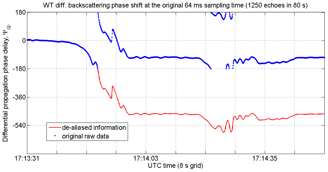
Figure 6 Representation of the variability of the differential phase shift measurable (see Sect. 2.3.4) at the highest available temporal resolution, namely 64 ms. The abscissa spans an interval of exactly 80 s (from 17:13:31 to 17:14:51 UTC, P2b); vertical lines on the x axis represent every 8 s, which correspond exactly to 125 echoes. Every 64 ms radar echo (measurable) has been derived by means of 128 pulses transmitted using a pulse repetition frequency of 2000 Hz. The blue dots correspond to the raw (aliased) data, while the red lines show the proper evolution of the signal. Since the radar receiver was stable in phase and amplitude and since there was no precipitation, changes in the differential phase shift, Ψ_dp, can be attributed to changes in the differential backscattering coefficient, δ_co.

This fact can be seen in Fig. 6, which shows the large changes in the differential phase shift at the original 64 ms sampling time: the changes in the differential phase shift, Ψ_dp, are characterized by long sequences of (high-frequency) negative discrete derivative values which bring Ψ_dp from the original (equilibrium) value not far from 0^∘ down to the new (equilibrium) value of −466^∘. In Fig. 6, the original aliased values (between ±180^∘) recorded by the radar are shown using blue dots, while the more meaningful de-aliased curve is shown using a solid red line that links all the points.

During the 32 s (17:12:59–17:13:31 UTC) just before the starting time of P2b, Ψ_dp was oscillating between +11 and +5^∘, while during the initial 200 echoes (12.8 s) of P2b, Ψ_dp monotonically decreased to approximately −20^∘. Then the slope of the decay started to increase until a relative minimum of −369^∘ was reached at echo no. 355 (the slope decreased to 0, obviously). Exactly in correspondence with the first, longer (nine consecutive 64 ms echoes) and deeper (down to 0.9803, which is DN = 250) drops of ρ_HV, Ψ_dp started to increase again up to −290^∘. Then, a rapid decrease down to −466^∘ followed, which was reached around echo no. 425 (17:13:58.2 UTC​​​​​​​). In the original, aliased data delivered by the radar signal processor, −466^∘ corresponded to a value of −106^∘. Except for a few oscillations between 17:14:13 and 17:14:35 UTC, the new equilibrium value was kept until 17:17:37 UTC, when a new significant change started.

Adding up, during sup-period P2b (17:13:31–17:14:51 UTC), something caused

• (large) changes in (Z_V) Z_H that, combined, caused an extreme variability of Z_dr, with a maximum of +30 dB;

• the consequent Z_dr transition from a large value of ∼ 16 dB to a value close to 0 dB;

• the transition of Ψ_dp (actually of the differential backscattering phase shift, δ_co) from ∼ 0 to −466^∘.

It could be related to the change in the blade pitch angle from 70 to 65^∘ and/or to the change of the nacelle orientation with respect to the radar (from 61 to 57^∘). Indeed, one important limitation of the present analysis is the very low temporal resolution (sampling time equal to 600 s) of the ancillary data associated with the WT: these data show that, even at zero rotor speed, other changes of the state of WT can have a large impact on the radar measurables.

Finally, the hypothesis that no change in the WT aspect happened between 17:13:58 to 17:14:18 UTC is plausible: the standard deviation of Ψ_dp was as small as 3.1^∘; this is typical for a still bright scatterer (see, e.g., Sect. 2.3.4​​​​​​​ and Sect. 3.6 in Gabella, 2018). Similarly, from 17:14:43 to 17:14:51 UTC, namely the last 8 s in Fig. 6, the standard deviation of Ψ_dp was 3.6^∘.

3.3 Period P3 (17:20–17:30 UTC): 22.5 rotor revolutions, blade pitch angle changed from 65 to 15^∘

During period P3, the average 10 min value of r_s was 2.25 rpm, which implies 22.5 revolutions. As far as the blade pitch angle is concerned, it decreased from 65 to 15^∘. The whole P3 was characterized by heavy fluctuations of ρ_HV, which never reached the value of 1 (green curve in Fig. 3). Regarding the fluctuations of the maximum and minimum reflectivity values of both polarizations (green and blue curves in Figs. 2 and 4), they were smaller between 17:23 and 17:28 UTC; our hypothesis is that, during these 5 min, the rotation was faster than the 10 min average, while before 17:23 UTC and after 17:28 UTC, only a partial, slow rotation was occurring, similarly to the one before 17:20 UTC. Thanks to the larger rotor speed, radar estimates were obtained over a larger rotation angle; this lead to a more stable median value of both Z_h and Z_v, as can be seen in Figs. 2 and 3. During this period with efficient rotor speed for energy production, both polarizations showed median reflectivity values around 58 dBz; the median Z_dr was around the neutral value of 0 dB.

It is particularly interesting that, while the rotor was probably slowing down (precisely at 17:29:31.729 UTC), Z_H reached 77.5 dBz, the third maximum value of the whole campaign. The third maximum value of Z_V could be identified 320 ms earlier (five echoes back in time). During P3, the nacelle orientation changed from 57 to around 10^∘, where it remained in the successive 10 min (period P4; see Sect. 3.4).

3.4 Period P4 (17:30–17:40 UTC): blade pitch angle back to 70^∘ and another partial rotation

During the quasi-steady 17:30–17:40 UTC interval, the average rotor speed was 0.06 rpm; this means that, overall, the rotor turned by only a 0.6 rotation, which is 216^∘. In Sect. 3.2 we assumed that the partial rotation of 72^∘ took place only after 17:17:17 UTC (and before 17:20 UTC); similarly, here we assume that the 216^∘ degree rotation was anyhow completed around 17:39:40 UTC, when the value of ρ_HV became persistently equal to 1 once again (see Fig. 3). It is worth noting that the absolute maximum reflectivity value of the whole campaign (78.5 dBz) was detected in four 64 ms echoes at such a very low rotor speed. The four 64 ms echoes belonged to only two different 8 s intervals (two absolute peaks in the green curve in Fig. 2). In both cases, the two 64 ms echoes were consecutive: the first pair was at 17:31:29.167 and 17:31:29.231 UTC (the corresponding Z_dr values are 4.5 and 4.0 dB); the second pair was at 17:35:53.367 and 17:35.431 UTC (the corresponding Z_dr values are 5.5 and 6.0 dB). The nacelle orientation was around 10^∘, which was one (among several) 10^∘ bin where the absolute maximum of 78.5 dBz was recorded during the campaign; other orientations involved were around 110, 170, 260 and 340^∘, as the reader can see in Fig. 10a of Lainer et al. (2021).

It is interesting to note that the slow rotation corresponded again to larger fluctuations of the maximum, median and minimum reflectivity values of both polarizations, as described in Sect. 3.3 for the first 3 min.

Around 17:39:40 UTC, the rotor probably stopped its rotation (ρ_HV often equal 1).

• Z_v was bounded between 53.5 and 55.5 dBz; (randomly smaller than the median of the energy production WT mode, for instance, between 17:23 and 17:28 UTC – see Sect. 3.3).

• Z_h was bounded between 45.5 and 47.0 dBz (also randomly smaller the median of the 5 min energy production mode).

• Consequently, the median differential reflectivity of this 0 rotor speed interval was around −8.0 dB.

4 Discussion

In this preliminary investigation, we have thoroughly analyzed 30 000 polarimetric echoes acquired in 32 min, during which the WT rotor accomplished 23.3 rotations. Thanks to the 10 min ancillary information regarding the WT, we know that the rotor speed was exactly zero during the first 2 min. It is also very likely that rotor speed was zero during the last 20 s (from 17:39:40 to 17:40:00 UTC; see Figs. 2–5). If compared to its ordinary rotation conditions, a still WT is much easier to be identified and rejected as clutter. This is something that has been known for a long time. The deep and detailed analysis presented here shows something novel in view of the emerging interest in BSs as an additional source of information for monitoring dual-polarization weather radars and meteorological applications (e.g., for assessing the path integrated attenuation of a melting hail cell; see Gabella et al., 2021). Indeed, the current polarimetric signatures of the still WT are similar to those of a BS in terms of very small dispersion of both the co-polar correlation coefficient, ρ_HV, and the differential phase shift in addition to the large average and median values of ρ_HV. The dispersion is even smaller and the central value even closer to the unity asymptotic limit than for the BS investigated at the C-band with a rotating antenna in a previous study. We hypothesize that such an effect can be due to the special stare-mode antenna scan program: all the 128 averaged pulses refer to an antenna beam axis that is pointing in the same geometrical direction. Residual sources of variability are then only fluctuations of the tropospheric refraction index and small movements of the blade tips. Similarly, for a still WT, the dispersion of both dual-polarization reflectivities and differential reflectivity is also much smaller than any other moving conditions.

Furthermore, with this preliminary study, it was possible to identify other WT configurations which cause quite different polarimetric signatures with respect to the simple still WT condition:

• a.

  The first distinctive configuration is zero rotor speed and probably no change in either blade pitch angle or nacelle orientation. This was surely the case from 17:08 to 17:10 UTC, period P1 (see Figs. 2–5 and Sect. 3.1); however, this configuration probably lasted until 17:13:31 UTC (see Sect. 3.2). Our hypothesis is that it happened again in other two intervals, namely between 17:14:41 and 17:17:37 UTC (see Sect. 3.2) and during the last 20 s before 17:40 UTC (see Sect. 3.4), as can be deduced from Figs. 2 to 5.

• b.

  Another distinctive (and probably rare) configuration is the one described in the central part of Sect. 3.2, as well as in Fig. 6, and that occurred between 17:13:31 and 17:14:41 UTC during the sub-period P2b – see Fig. 2. It could have been caused by a change in the blade pitch angle while the rotor speed was still zero. This is just a plausible hypothesis. Whatever the reason could be, the changes in the differential backscattering coefficient, δ_co, are quite significant (see Fig. 6).

• c.

  Then the most usual configuration comes, which is the one of energy production under sufficient wind conditions. We think that it lasted approximately 5 min (say from 17:23 to 17:28 UTC) during which most of the 22.5 rotations of period P3 occurred.

• d.

  Finally, there is a configuration that is associated with large variability of the parametric signatures (from 17:17:37 UTC to approximately 17:23 UTC and, most of all, from approximately 17:28 to 17:39:20 UTC – see Sect. 3.4).

Regarding (a), we conclude that, when the rotor speed is zero, the WT signatures are similar to those of a bright scatterer: we have observed, in fact, a good stability and small dispersion of the polarimetric variables; the situation is even better than what has been observed with a rotating antenna (18^∘ s⁻¹) by Gabella (2018) using the metallic tower of Cimetta at a range of 18 km from the Monte Lema C-band radar. The even larger stability and small dispersion in the present campaign are due to the antenna stare mode of the X-band radar. A very small dispersion of the polarimetric variables is also observed in the intervals from 17:10:00 to 17:17:40 UTC and from 17:39:40 to 17:40:00 UTC. Our guess is that, in both cases, the rotor speed was equal to zero, which is exactly the status of the previous (17:00–17:10 UTC) and following (17:40–17:50 UTC) 10 min intervals. A preliminary analysis of a different case (about 90 min of radar data collected on 19 March 2021) not included in the present paper has also shown ρ_HV values always equal to 1. For this case, the three operational parameters of the WT (nacelle orientation, pitch angle of the blades, rotor speed) heavily affecting the backscattering signatures did not change: in particular, rotor speed was always zero in the interval of interest.

Regarding (b), let us focus again on the 1000 radar polarimetric values acquired in the 64 s of the sub-period P2b (see Fig. 2), namely from 17:13:31 to 17:14:35 UTC: one can easily see large changes in both the horizontal (Fig. 2) and vertical (Fig. 4) polarization reflectivity (and consequently the extreme variability of Z_dr, reaching an extreme maximum of +30 dB and a minimum of +4.5 dB – see Fig. 5); a transition of Z_dr from a large value of +16 dB to approximately 0 dB; and a transition of the differential phase shift, Ψ_dp, from around ∼ 0 to −466^∘, probably caused by an overall change of 466^∘ in the differential backscattering phase shift. What could be the cause of such simultaneous large changes in Z_dr and Ψ_dp? It could be a change in the blade pitch and/or nacelle orientation. Was there also a small movement of the rotor? It is hard, if not impossible, to find an answer to such questions with the present data. For future campaigns, it is obvious to recommend a much better (smaller) sampling time regarding the WT status and wind information: ideally, from the current 600 s down to 1 s or less. Another obvious recommendation is related to the quantization of ρ_HV, specifically the use of two bytes or a log-transformation – like, for instance, the operational one used at MeteoSwiss (see Eq. 6 in Gabella, 2018).

There are two other facts worth mentioning. The first one is a sort of intrinsic inverse correlation between the dispersion and the central value of the co-polar correlation coefficient among many consecutive 64 ms echoes. When ρ_HV is close to the asymptotic value of 1, then the changes among successive echoes tend to be very small (see Fig. 3 – from 17:30 to 17:40 UTC, partial rotor rotation of 216^∘ in 10 min). As stated, when the rotor does not move and the blade pitch angle and orientation do not change, then ρ_HV is consistently and constantly equal to 1; this fact was confirmed by analyzing 86 250 high-temporal-resolution echoes on 19 March 2020.

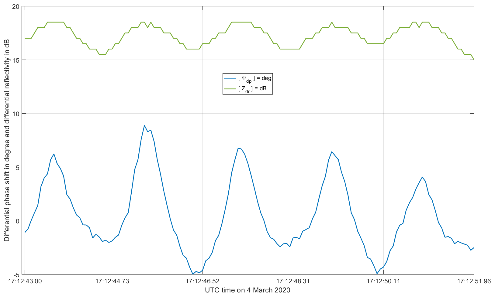
Figure 7 An example of quasi cycle stationarity of both the differential reflectivity in dB (green line) and the differential phase shift in degree (blue line) at the highest available temporal resolution, namely 64 ms. The abscissa spans an interval of exactly 8.96 s, which corresponds exactly to 140 echoes of the selected interval P2a. Vertical lines represent every 1.792 s, which is 28 consecutive echoes.

The second fact is an occasional, short-lasting, quite surprising correlation between the differential phase shift (fourth measurable – see Sect. 2.3.4) and the differential reflectivity (second measurable – see Sect. 2.3.2) associated with a sort of cyclo-stationarity (although during very short intervals): this fact can be seen, for instance, during the 8.96 s (140 echoes) displayed in Fig. 7, during which approximately five periodic cycles of the two polarimetric measurable took place. In Fig. 7, the vertical lines represent every 28 echoes (1.792 s); obviously, our intention is not to claim that the period is exactly 1.792 s since 1.728 s (27 echoes) is certainly another reasonable estimate.

We think it is interesting to emphasize that there must be something WT related within a period of ∼ 1.7–1.8 s, which is reflected in both the (differential) phase and the (differential, squared) amplitude of the polarimetric signals received by the radar.

5 Summary, conclusions and outlook

This technical note has extended the analysis and investigation by Lainer at al. (2021) in two directions:

1. to complement the statistics of the horizontal polarization radar reflectivity factor with those corresponding to other polarimetric measurables: the co-polar correlation coefficient, ρ_HV; the vertical polarization reflectivity factor; the differential reflectivity, Z_dr; and the differential phase shift, Ψ_dp, between the phases of the co-polar signals at horizontal and vertical polarizations

2. to investigate the variability of the polarimetric measurables at the best available temporal resolution (sampling time as short as 64 ms) despite the precious and valuable ancillary data related to the wind turbine status being available only every 600 s.

We have tackled the challenging sampling time (600 s vs. 0.064 s) problem by starting with an interval that was characterized by zero rotor speed (still wind turbine). In such a distinctive case of still WT, we have observed the following:

• ρ_HV is perfectly stable and always equal to 1 (DN = 255).

• It is the case that 38.5 dBz ≤ Z_v ≤ 41.5 dBz – i.e., only seven digital numbers are used; the standard deviation is as small as 0.725 dBz. By way of example, note that from 04:00 to 04:10 UTC on 19 March, it was 53.0 dBz ≤ Z_v ≤ 54.5 dBz. Hence, Z_v has shown a smaller variability and was constant during several seconds.

• Since Z_h is always equal to 56.5 dBz (see Sect. 3.1), the temporal variability of Z_dr is identical to that of Z_v (just with the opposite sign, obviously). Similarly, from 04:00 to 04:10 UTC on 19 March, it was 54.5 dBz ≤ Z_h ≤ 55.5 dBz. Furthermore, Z_h was constant for several minutes.

• For both Z_h and Z_v, the interesting fact to note is the very small range of variability of the still WT, which acts as a bright scatterer. As expected, such extreme stationarity of the backscattered signal by a BSs cannot be obtained with a rotating antenna (see, e.g., Gabella, 2018).

• It is the case that 4^∘ ≤ Ψ_dp ≤ 40^∘ during a 2 min interval, with periodic oscillation of approximately ±3^∘ in a bit less than 2 s; the standard deviation is as small as 2.9^∘.

The large difference in sampling time (64 ms vs. 600 s) certainly poses a challenge to future analyses of the valuable 3-week campaign in March 2020. Nevertheless, we plan to extend this (32 min) analysis (based on 30 000 polarimetric measurables) to a distinctive day (19 March 2020), which is characterized by several 10 min intervals with zero rotor speed. As stated, a preliminary analysis over 92 min has shown similar results: ρ_HV is always equal to 1, and there is small dispersion of the radar reflectivity factors.

The prevailing-in-time stare-mode acquisition of the 2020 campaign has been proven to be highly beneficial for a better characterization of the polarimetric signatures of the wind turbine, especially when it is still (or quasi-still): the stability of the measurements at the still turbine proves the good quality of the campaign. The results from previous single-polarization studies (Lainer et al., 2021) are confirmed: the rotor speed is a key piece of information for the prediction of the values, the variability of backscattered power, and the phase of horizontal and vertical polarizations. Another important parameter is the rotor blade pitch angle, which probably changes in a relatively short time (much shorter than the 600 s sampling time of the turbine data obtained so far). At the moment, what is more difficult to assess is the dependence on the nacelle orientation. Surely, we are just at the beginning of the fascinating task of deriving spectral and polarimetric signatures of wind turbines from the point of view of a weather radar, keeping in mind that the special results of the present experiment were possible thanks to the stare-mode scan strategy. An operational radar with a rotating antenna will retrieve variances of the polarimetric signatures that are affected by both changes: those of the WT (blade rotation) and those of the radiation pattern (antenna rotation).