Segmentation of polarimetric radar imagery using statistical texture

Weather radars are increasingly being used to study the interaction between wildfires and the atmosphere, owing to the enhanced spatio-temporal resolution of radar data compared to conventional measurements, such as satellite imagery and in situ sensing. An important requirement for the continued proliferation of radar data for this application is the automatic identification of fire-generated particle returns (pyrometeors) from a scene containing a diverse range of echo sources, including clear air, ground and sea clutter, and precipitation. The classification of such particles is a challenging problem for common image segmentation approaches (e.g. fuzzy logic or unsupervised machine learning) due to the strong overlap in radar variable distributions between each echo type. Here, we propose the following two-step method to address these challenges: (1) the introduction of secondary, texture-based fields, calculated using statistical properties of gray-level co-occurrence matrices (GLCMs), and (2) a Gaussian mixture model (GMM), used to classify echo sources by combining radar variables with texture-based fields from (1). Importantly, we retain all information from the original measurements by performing calculations in the radar's native spherical coordinate system and introduce a range-varying-window methodology for our GLCM calculations to avoid range-dependent biases. We show that our method can accurately classify pyrometeors' plumes, clear air, sea clutter, and precipitation using radar data from recent wildfire events in Australia and find that the contrast of the radar correlation coefficient is the most skilful variable for the classification. The technique we propose enables the automated detection of pyrometeors' plumes from operational weather radar networks, which may be used by fire agencies for emergency management purposes or by scientists for case study analyses or historical-event identification.

1 Introduction

The ability to analyse large wildfire (referred to as “bushfire” in Australia) behaviour in real time remains one of the biggest challenges in wildfire incident and risk management. Physical processes happen at various spatio-temporal scales, from the smaller scale of fuel consumption, heat, moisture, and pyrogenic emissions to larger-scale vortices, downdrafts developing in the smoke plume column, and associated clouds. Large wildfires are often topped by pyrocumulus or pyrocumulonimbus (pyroCb) clouds. The dynamics and microphysics of these clouds usually evolve very rapidly, including the formation of strong updrafts and downdrafts and their associated hazards. Pyrogenic smoke plumes and clouds facilitate the transport of embers that could light new fires when landing and generate lightning that could ignite new fires in the case of pyroCb. Yet, our ability to observe wildfire behaviour with the high temporal resolution provided by satellite-based passive sensing technologies remains limited because pyrogenic particles often obscure the fire ground and lower levels.

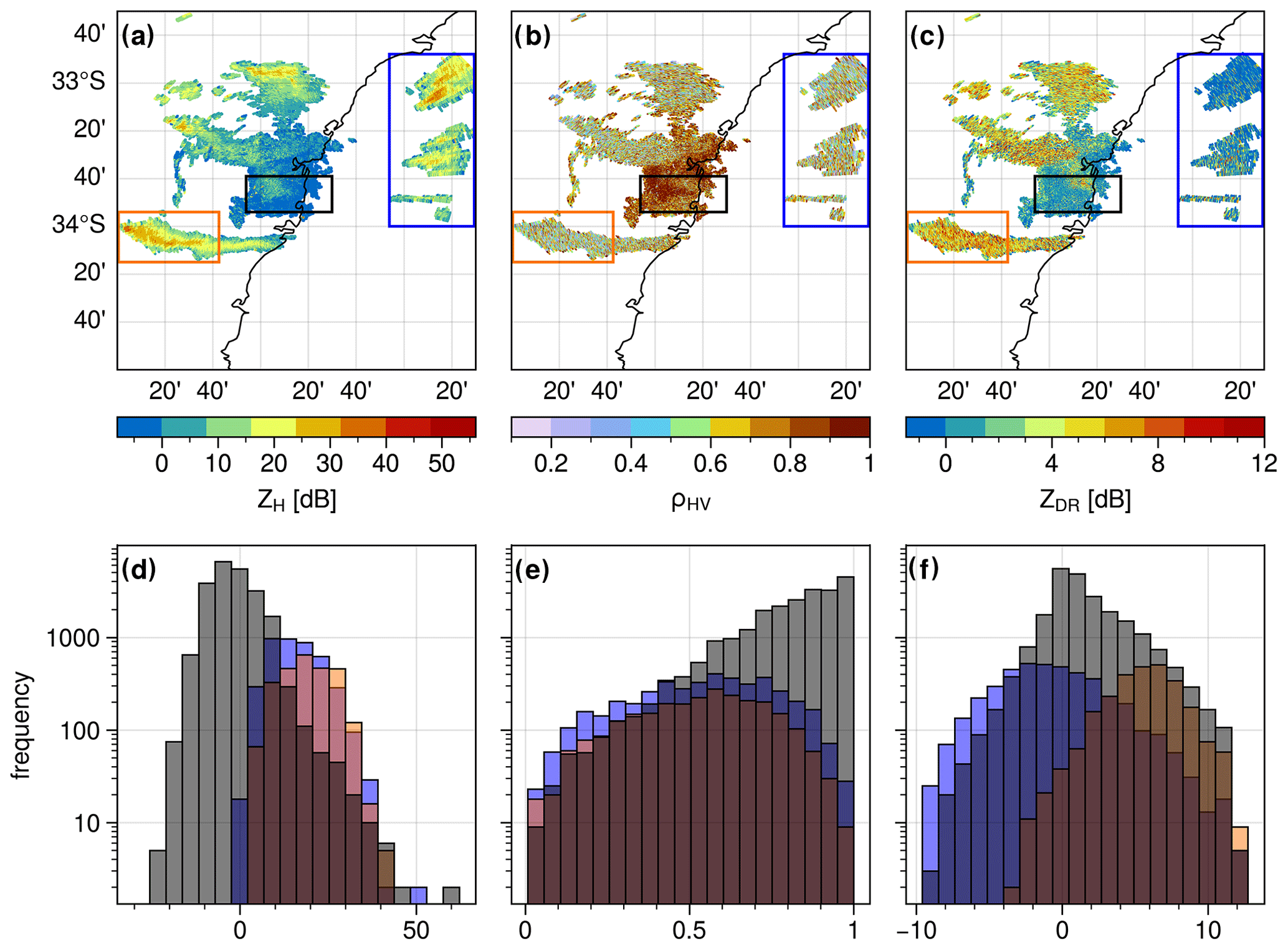
Figure 1 Polarimetric weather radar fields for the second tilt at 0.9^∘ elevation from the S-band radar of Terrey Hills, Sydney, for 29 November 2019 at 05:07 UTC: spatial and frequency distributions of the horizontal reflectivity (a, d), correlation coefficient (b, e), and differential reflectivity (c, f). Red, black, and blue contoured boxes (a–c) correspond to pyrometeors, clear air (possibly including remaining ground clutter), and sea clutter echoes, respectively. The same colour coding is used in the histograms in subplots (d–f). Hotspots (for fire radiative power > 100 MW; acquisition time 04:29 UTC) derived from MODIS (sourced from Fire Information for Resource Management System – FIRMS; Giglio et al., 2016) are plotted as red squares in panel (a).

To address the spatial intelligence gap, following an earlier work of Duff et al. (2018), Lareau et al. (2022) proposed using weather radar when available to indirectly track fire progression via radar reflectivity. Weather radars can observe ash and large debris emitted by wildfires and transported aloft; this range of wildfire-borne scatterers producing weather radar echoes has been collectively denoted as “pyrometeors” (McCarthy et al., 2018; Kingsmill et al., 2023). Conversely, “wildfire smoke” encompasses all wildfire-borne particles, including both pyrometeors and aerosols of smaller sizes. Lareau et al. (2022) developed an algorithm to derive fire perimeters based on real-time radar reflectivity maxima. This method was tested with US Next Generation Weather Radar data for two large wildfires that occurred in northern California. The authors showed this method would benefit from being tested and applied to several large wildfires within operational weather radar coverage. More generally, weather radar remains an under-utilised observational tool despite meeting the required criteria for wildfire tracking at a high temporal resolution (typically 5 min for operational weather radars) and high spatial resolution (from 50 to 1000 m depending on the radar distance to the fire ground and radar characteristics).

The first step before applying an algorithm, such as the one proposed by Lareau et al. (2022), is to identify and segment pyrometeors' plumes and associated clouds within a weather radar volume. Often, during a wildfire event, a range of weather radar signal returns is present within a plan position indicator (PPI) scan, in addition to the pyrometeors' plume, such as ground, clear-air, and sea clutter, precipitation, insects, or biological returns. Figure 1 shows an example of such a complex scene for wildfire pyrometeors' plumes near Sydney during the 2019/20 Black Summer wildfires. Several pyrometeors' plumes can be seen extending from the fire area in the west towards the east and stretching over more than 100 km. In that imagery, clear-air returns are clearly visible within a 50 km radius of the weather radar location. While a clutter removal algorithm has been applied to the data (Gabella and Notarpietro, 2002), some ground clutter likely remains due to anomalous propagation conditions occurring on that day, similarly to what was observed in Melbourne under similar conditions (Guyot et al., 2021). Sea clutter is also present to the south and the east of the radar (blue coloured box in Fig. 1). One can also distinguish a few showers in the southwest. Extracting the weather radar returns from pyrometeors only is particularly difficult when the pyrometeors' plume is within the 50 km radius of the radar, as clear-air and pyrometeors' echoes are intertwined. Conversely, classification of precipitation is more straightforward since its polarimetric signatures have unique characteristics.

Fuzzy-logic or unsupervised clustering-based approaches based on polarimetric radar variables are commonly used for weather radar echo classification (Berenguer et al., 2006; Marzano et al., 2007; Zrnic et al., 2020). For these methods to be effective, each radar echo class needs to occupy a distinct area in the multi-dimensional space defined by all the input parameters with as little overlap as possible so that robust membership functions can be established (in the case of fuzzy-logic approaches) or synthetic models can be developed (in the case of unsupervised learning such as a Gaussian mixture model). In the example shown in Fig. 1, a classification based on the reflectivity (Z_H, dBZ), correlation coefficient, and differential reflectivity seems very difficult due to the largely overlapping distributions of these variables for clear air, pyrometeors, and sea clutter. For instance, the pyrometeors–clear-air boundary is difficult to define (Fig. 1a and d). Another example of an overlapping distribution is the co-polar correlation coefficient (ρ_HV, unitless) values, which tend to produce very similar distributions for pyrometeors and sea clutter, whereby the values of ρ_HV show higher frequencies of values in the upper range (above 0.6), with a strong overlap with pyrometeors and sea clutter. Differential reflectivity (Z_DR, dB) values are more likely negative for sea clutter but with positive values as well, while the clear-air distribution is centred around 0 dB and pyrometeors show more frequency in the higher range, up to 13 dB (the maximum value in the Australian operational network). The presence of sea clutter is produced by anomalous propagation conditions due to temperature inversion, conditions often present over large waterbodies, further enhanced here by the presence of smoke (Guyot et al., 2021). Despite these difficulties, a trained radar scientist could easily differentiate the different echoes from that complex scene. The main challenge here is to automatically discriminate these different echoes and objectively separate clear air from pyrometeors when these are intertwined.

While widely used and providing very good results for the segmentation of precipitation and clear air, fuzzy-logic and clustering approaches do not make use of the spatial relationship between nearby radar bins (or pixels in the images). In this paper, we propose a new method for the segmentation of pyrometeors' plumes based on the combination of a textural approach (gray-level co-occurrence matrices) and an unsupervised machine learning approach (Gaussian mixture model). The paper is organised as follows: we first describe the methods and then evaluate the effectiveness of our new technique using operational weather radar data from several wildfires that occurred in Australia during the 2019/20 Black Summer.

2 Methods

2.1 Texture fields based on gray-level co-occurrence matrices

Various methods have been proposed to quantify the texture, i.e. the spatial arrangement of intensities, of an image (Li et al., 2014). First-order statistics consist of simply deriving the mean or variance of distributions of values within an image. These features can be computed globally, i.e. deriving single values for the whole image, or locally, i.e. deriving values for each pixel by applying a moving window and allocating feature values to the centre pixel. These first-order statistics only reflect the distribution of intensity levels in an image (Haralick et al., 1973) and do not preserve the directionality of the intensity distribution.

A widely used method in texture analysis proposed by Haralick et al. (1973) relies on the computation of gray-level co-occurrence matrices (GLCMs) from which Haralick features can be calculated. Recent applications include medical image analysis, in particular magnetic resonance imaging (MRI) or ultrasound for the detection of cancers (Chitalia and Kontos, 2019; Yang et al., 2012). However, GLCMs have also been used extensively in the analysis of satellite imagery since it was first proposed by Haralick in 1973 (Hall-Beyer, 2017). The first step in the GLCM approach is to re-scale the original image (with values ranging from k to l) to a new quantised image (with integer values ranging from 0 to N). This important step can be optimised to reduce the GLCM computational time, as the smaller the range [0, N], the faster the computation. However, care must be taken if reducing the range past a certain value of N as information contained in the original image will be lost. It must also be noted that different values of N will lead to different values of GLCMs and their Haralick features, so the reproducibility of the results strongly depends on that chosen N value. Löfstedt et al. (2019) discussed this issue in detail and proposed a gray-level-invariant approach to retrieve texture feature values independently of the image quantisation. To optimise the computational efficiency of our application, we decided not to implement this approach.

In a second step, the GLCMs are computed by counting how many times each pair of pixels of the same value (for a given gray level) occurs within a given window surrounding the central pixel. The neighbour of a pixel is defined by a vector of angle θ and distance d. The GLCM can be defined as in Eq. (1):

$$\begin{array}{}\text{(1)}& X(i,j)=\sum _{m=\mathrm{0}}^M\sum _{n=\mathrm{0}}^N(\mathrm{1}\text{ if pixel identical},\mathrm{0}\text{ otherwise}),\end{array}$$

where X is the GLCM of elements (i,j) and m,n is the quantised given window. For each displacement vector (combination of (d,θ)) a GLCM can be calculated. To cover all directions surrounding a central pixel, eight angles should be used, but displacement vectors of opposite angles will lead to symmetric GLCMs; therefore only four angles are necessary to cover all the possible variations (θ = 0, $\mathit{\pi }/\mathrm{4}$, $\mathit{\pi }/\mathrm{2}$, $\mathrm{3}\mathit{\pi }/\mathrm{4}$). We also consider two distances (d=1, d=2), resulting in eight displacement vectors in our study. We discuss the sensitivity of the results to these choices in Sect. 3.2.

In the third step, the original GLCM is normalised so that all elements of the matrix represent the probability of each combination of pairs of neighbouring pixels occurring for the given window over which the GLCM was calculated. This normalised GLCM is calculated as in Eq. (2):

$$\begin{array}{}\text{(2)}& P_i={\displaystyle \frac{X_i}{\sum _{i=\mathrm{0}}^{K-\mathrm{1}}{X}_i}},\end{array}$$

where i is the pixel number, P_i is the probability recorded for the cell i, and K is the total number of pixels.

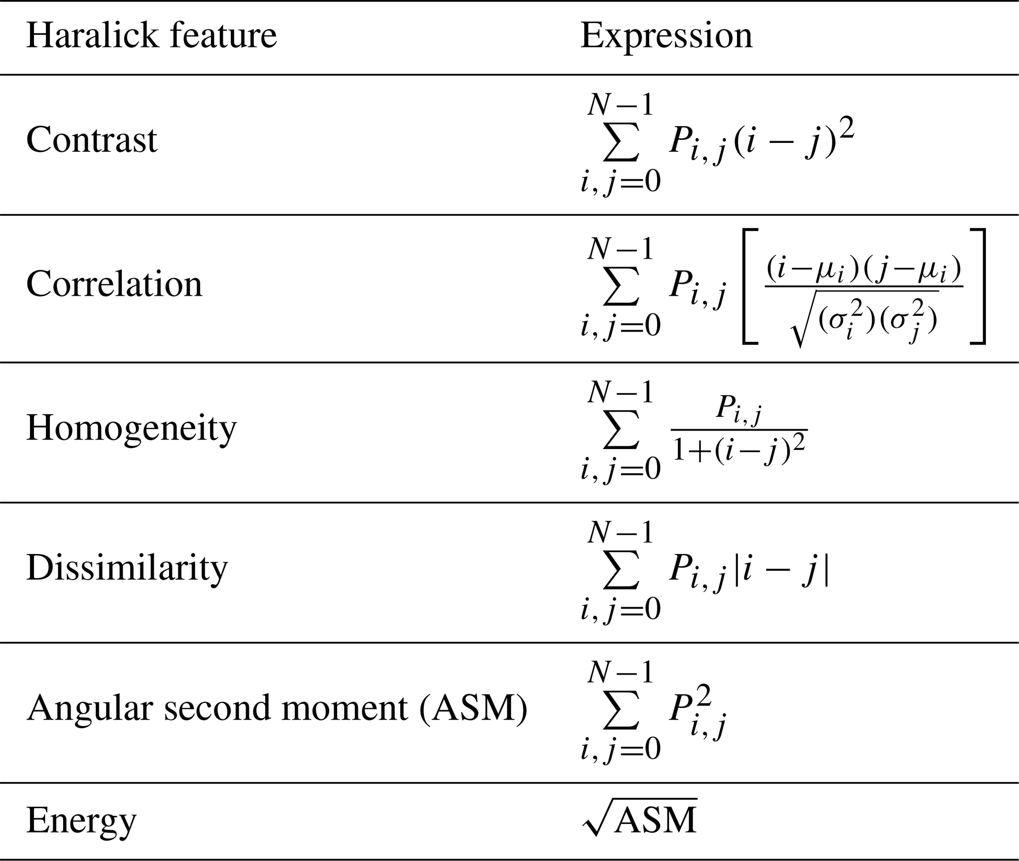
Finally, in the last step, we computed the Haralick features from the normalised GLCMs. Originally, Haralick et al. (1973) proposed 14 different features to be calculated from the GLCMs. Here, we chose to restrict ourselves to the six most used features (and conduct a comparison of these for synthetic and real data to see if these could be reduced further. The six chosen features together with their mathematical expressions are shown in Table 1. Each feature can be calculated for each combination of (angle, distance), leading to eight values for a single feature. A common approach used widely is to take the mean (from eight values) of each of the features (Löfstedt et al., 2019), this being referred to as a spatially invariant measure (given this is the average of the four possible directions). We decided to explore the effect of directionality on the retrieved features by comparing these eight different retrievals, and we also computed the mean and the standard deviation of the eight values.

Table 1 Selected texture Haralick features utilised in this study together with their mathematical expressions. All six features are unitless.

2.2 The spherical representation of weather radar data

The mode of acquisition of weather radar data, scanning and receiving from the same antenna, and the scanning strategy dictate that the resulting data are distributed in the three-dimensional space where each grid point can be described in polar coordinates (elevation, azimuth, range). In this article, we perform our calculations on two-dimensional, plan position indicator (PPI) scans in their native spherical coordinates. We consider position plan indicators plane (two-dimensional) surfaces that correspond to a given elevation and its full range of azimuthal and range values. For each of the radar variables, a PPI can be considered a two-dimensional “image” with the x axis as the range and the y axis as the azimuth. However, the spatial resolution of these images varies considerably along the y axis because of beam broadening with range. Typically, for a radar with a beam width of 1^∘ and a range gate size of 250 m, the approximate area covered by a pixel at 1 km range is 4909 m², while the area covered by a pixel at 100 km range is 10 000 times larger (the area is proportional to the square of the distance). Weather radar data can be gridded using various methods (e.g. Brook et al., 2022; Trapp and Doswell, 2000); however, these methods necessarily smooth the underlying radar fields and may strongly influence the resulting texture calculations. For this reason, we restrict our texture analysis to data collected in the radar's native spherical coordinates. Typically, the correlation coefficient or differential reflectivity fields can show boundaries in space when the observed medium includes rain or hail. Clear air, sea clutter, and pyrometeors all exhibit very spatially variable signatures (appearing as “noisy”) in two-dimensional space. Interpolating native weather radar polarimetric variables on a regular grid and necessarily smoothing these fields would impact the retrieved texture, likely reducing its absolute local values and modifying its spatial pattern.

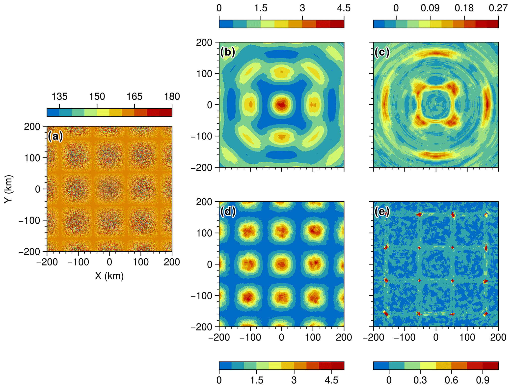
Figure 2 (a) Synthetic field; (b) GLCM mean texture of the synthetic field as shown in (a) with a fixed window size of 20; (c) GLCM mean correlation of the synthetic field with a fixed window size of 20; (d) GLCM mean contrast of the synthetic field with a varying window size; (e) GLCM mean correlation of the synthetic field with a varying window size.

Several authors have employed texture analysis for image classification on weather radar fields. Chandrasekar et al. (2013) reviewed the methods used in classification, including early work on texture. Giuli et al. (1991) and Schuur et al. (2003) applied first-order statistics such as the mean and standard deviation over a 3 × 3 window (three azimuths, three ranges) for Z_DR, Z_H, and the differential phase. Gourley et al. (2007) proposed to use the root-mean-square difference between pixels within a 3 × 3 window, effectively a first-order statistic, as it does not consider pixel interdependency, i.e. relations in space between pixels of the same values. More recently, Stepanian et al. (2016) and Jatau et al. (2021) utilised variance over a 5 × 5 pixel neighbourhood for Z_DR, and the root-mean-square deviation of the differential phase over 9 pixels in the range. All these authors used radar data in polar coordinates; Gourley et al. (2007) noticed the range dependency of texture fields. Their Z_DR texture field decreased with range close to the radar, where noisy values of Z_DR are more common due to clutter. Conversely, the Z_DR texture field increased in value at long range due to the natural variability in Z_DR. This is contradictory to the description of Stepanian et al. (2016), who stated that as the beam width of sampling volumes increases with range, more scatterers contribute to the volume, thereby increasing the intra-volume variability. Increasing the sample size leads to a more accurate representation of mean values for volume at longer range, less pixel-to-pixel variability, and therefore smaller values of the texture at longer range. Lakshmanan et al. (2003) used the homogeneity of Z_H, where homogeneity is calculated from the co-occurrence of the pixel of the same value within a given window (similarly to GLCMs). The authors did not discuss range effects in polar coordinates and present only succinct results where such an effect cannot be observed. Finally, Oliveira and Filho (2022) explored the application of a gray-level difference vector (GLDV) to gridded rainfall data derived from weather radar. The advantage of GLDVs over GLCMs is significant improvements in computational time. This is because the two dimensions of the GLCMs are reduced to a single vector of the size of the quantisation. However, their results and interpretations based on gridded data are not directly transferable to polar coordinates.

Here, we propose an adaptation of the GLCM to polar coordinates by varying the window size along the axis tangential to the range axis. Indeed, if we consider a given PPI defined by its range and azimuth in polar coordinates, we can also see the PPI as an image with identical pixel sizes to the range as the x axis and the azimuth as the y axis. As shown previously, the radar volumes and their projected surface areas vary along the range axis as a function of the square of the range. We attempt to normalise the neighbourhood area for each GLCM calculation by including more pixels in the azimuthal direction at close range and fewer at long range. The slope of the window size variation shall be like that of the variation in the pixel surface area. We arbitrarily set a minimum window azimuthal width of 5 at long range, since a smaller window would lead to too few pixels to calculate a GLCM. We also set a fixed window range depth of 5; therefore the window at long range has a square shape (in image space). Based on these constraints, we derived a function providing the window width as a function of range. It should be noted that this approach does not fully account for object-scale effects that are inherent to changes in resolution with range. Typically, the radar can resolve objects (such as vortices) at closer range but suffers from spatial aliasing (used here in its general form, not to be confused with Doppler folding) due to non-uniform beam filling at longer range. Both the fixed-window and varying-window approaches are implemented on random noise data fields in order to evaluate the benefits of implementing a varying window. The synthetic field in polar coordinates was made of a repetitive pattern of circular shapes of randomly distributed Gaussian noise (Fig. 2a), with a radius of approx. 80 km each, so at least three discs will occur within the 200 km radius of the radar image. The implementation of the above algorithm was done in the Python language (Rossum, 1995) and run using multiprocessing and eight CPUs. Alternatively, GPU-based computing has been shown to be extremely efficient for specific tasks where parallel computing is possible. Typically, a single GPU can replace dozens to hundreds of CPU cores, as demonstrated by Häfner et al. (2021) for global ocean modelling applications, enabling faster and more energy efficient computations. The limitation of using GPUs is the possibility of the tasks being parallelised and the need to write the processing code specifically for GPUs. A future implementation of our approach using GPUs to improve computational time is discussed in the “Discussion and conclusions” section.

2.3 Segmentation of data with a Gaussian mixture model

Gaussian mixture models (GMMs) have demonstrated their efficiency for image segmentation, especially where no preconception about the probability distribution of the input features (or variables) is available. This method has also been used to classify hydrometeor types based on weather radar variables (Wen et al., 2015). Here, we employed the same approach as in McCarthy et al. (2020) to classify pyrometeors, i.e. the scatterers typically present in pyrometeors' plumes, using portable X-band weather radar data. As Wen et al. (2015) demonstrated, the probabilistic nature of the GMMs can account for any specificity of any given weather radar. It is a more objective approach than fuzzy-logic or decision tree approaches, which are based on preconceptions of the data structures. GMMs are a modified version of the k-means clustering method and, similarly to k-means clustering, require the number of clusters to be chosen by the user (the hyperparameter k). The k-means algorithm is improved by using the expectation maximisation (EM) method, which was introduced by Dempster et al. (1977). In this algorithm, the first step (the expectation step) estimates the probability of each data point belonging to one of the k distributions. These distributions are described by their mean and covariance across the input features (in this case, radar variables). In the second step (the maximisation step), the mean and covariance of the k distributions are recalculated based on the probabilities found in the first step. This results in models that can effectively capture multivariate datasets represented by ellipsoidal confidence functions, which can be used to probabilistically classify new data. The Gaussian distributions also form a generative model, allowing for the generation of random output samples based on the mean and covariance of the final maximisation step.

Here, GMMs are used as our second step for the segmentation of the 2D PPI field. Based on a sensitivity analysis, where all combinations of variables as inputs were tested (not shown), we retained the following variables as inputs to the GMM: the Haralick local feature “contrast” (Table 1) of the correlation coefficient variable (unitless), the Haralick local feature contrast for Z_DR, the range of the given radar bin (in metres), reflectivity, the correlation coefficient, and differential reflectivity. The GMM is used as an unsupervised classifier, so the model is trained and fitted to a dataset of interest, combining all successive PPIs into a single dataset. Two days have been selected to train the model: 29 November 2019, as this day included several occurrences of intertwined clear-air, sea clutter, and pyrometeors' returns, and 2 December 2019, as this day also included scattered showers moving eastwards over the pyrometeors and clear-air regions. These data from two dates allowed us to include all types of potential scatterers that could be present in the vicinity of the region, apart from hail, which was infrequent in the Sydney region over the 2019/20 Black Summer. The model is then applied to data that were not used as part of the training but that were known to contain pyrometeors: 11 November 2019 was chosen as that day also included the formation of a pyrocumulonimbus cloud, enabling us to evaluate if our method could distinguish the formation of rain droplets within the pyrometeors' plume.

Selecting the number of clusters for the GMM, i.e. an integer value for the hyperparameter k, can be done arbitrarily or chosen based on optimisation techniques. The traditional methods to assess the optimal value for k are based on minimising the values of the Akaike information criterion (AIC) or the Bayesian information criterion (BIC) (Vrieze, 2012). In practice, the model is trained and tested on the same dataset for a range of k values: in our case, we varied k from 1 to 10. The values of the AIC and the BIC should plateau for a threshold value of k, making that value the optimum number of clusters (past that number, some clusters will share very similar properties). However, Wen et al. (2015) and McCarthy et al. (2019) both showed that for GMMs applied to dual-polarised radar data, no plateauing was observed, possibly due to the very large size of the dataset (McCarthy et al., 2019) or the assumption of a mixture of Gaussian distributions for the data. In our study, we know that the minimum number of clusters (value of k) should correspond to different types of scatterers that we want to discriminate, namely clear air, ground clutter (if some is left after the clutter removal), sea clutter, pyrometeors, and hydrometeors. Using values of k above 4 could also be acceptable, as the same echoes could present different characteristics; for example pyrometeors could present various microphysical properties as in McCarthy et al. (2019), and hydrometeor classification schemes typically include several hydrometeor types to discriminate between rainfall, ice particles (pristine or aggregates or hail), and melting hydrometeors. In our case, if the BIC and AIC present strong declining gradients past k=4, a larger value for k will be retained. The Python-based scikit-learn package (Pedregosa et al., 2011) implementation of GMMs was applied.

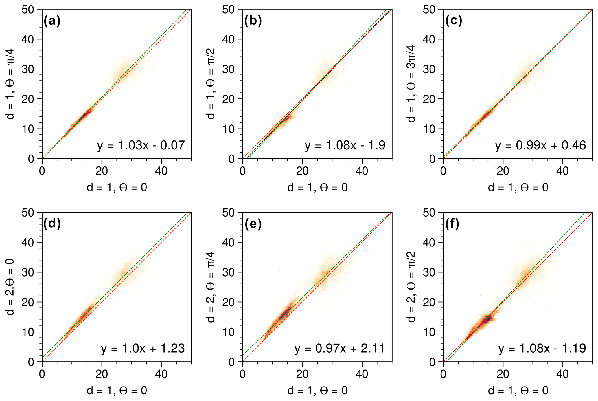
Figure 3 (a–f) Scatterplots of GLCM contrast values for different combination of distances (d) and angles (θ) for data from the Terrey Hills radar from 29 November 2019 at 05:07 UTC for ρ_HV at the second tilt (0.9^∘ elevation).

3 Results

3.1 Adaptability of GLCM to the spherical representation of weather radar data

To evaluate the effect of the weather radar range bin size on the retrieved GLCM features, synthetic data were utilised as an input to our GLCM algorithm. This is depicted in Fig. 2a, where the input data consist of evenly spaced clusters of random noise across the radar grid (polar coordinates), spanning a range of −200 to 200 km on both the x and the y axes. The values are distributed across the gray scale (0–255). The synthetic data assume a beam width of 1^∘ and a range gate size of 250 m, similar to the actual data from the Sydney (Terrey Hills) radar later used in the paper. In Fig. 2b, a fixed window size of 20 pixels was used to retrieve the contrast. The expectation is that the contrast of all pixels of the same size will be similar to the circle centred at coordinates x=0, y=0, since the pixels at very close range for polar coordinates are indeed very similar to one another. As the range increases, pixels become wider (their length stays the same along the azimuthal axis), and the effect of this can be clearly seen in the shape of the nine circles surrounding the central one. The circles at perpendicular azimuths (0, 90, 180, 270) are less distorted than the ones at azimuths (45, 75, 225, 315) because the distances to the origin are smaller, and the rate of increase along the perpendicular axis to the azimuth is larger. This effect is a clear issue as the retrievals will be range-dependent in terms of both the magnitude of the contrast and its spatial distribution. In Fig. 2d, the GLCM contrast was retrieved using a varying window size with range as previously described. The central circle is similar to the fixed window size, as the initial size of the window (win) is the same (win = 20 pixels). The nine circles surrounding the centre have different shapes and magnitudes than the ones shown in Fig. 2b. They all exhibit similar contrast values to the central circle, indicating that reducing the window size along the tangential axis to the range has enabled preservation of the shape of the retrievals.

In Fig. 2c and e, results for the GLCM correlation and its standard deviation are similar to those for the contrast, as indicated by the preservation of the spatial structure of the synthetic field and the consistent magnitude of peaks across the grid. These results support the moving-window approach as a robust approximation to apply GLCMs to data in polar coordinates, where the bin (pixel) size increases with range.

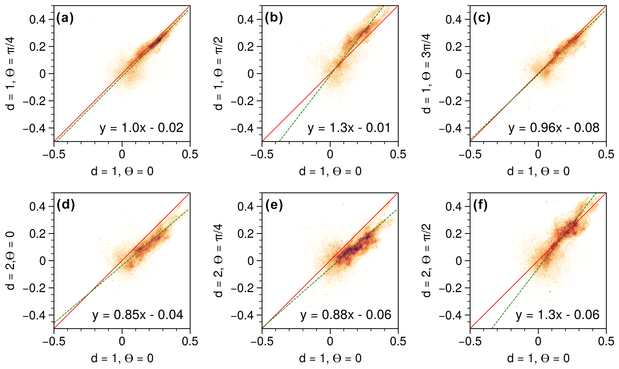
Figure 4 (a–f) Scatterplots of GLCM correlation values for different combinations of distances (d) and angles (θ) for data from the Terrey Hills radar from 29 November 2019 at 05:07 UTC for ρ_HV at the second tilt (0.9^∘ elevation).

3.2 Directionality and Haralick features of the GLCMs

A common practice in GLCM calculations is to take the mean of the four main directions (θ=0, $\mathit{\pi }/\mathrm{4}$, $\mathit{\pi }/\mathrm{2}$, $\mathrm{3}\mathit{\pi }/\mathrm{4}$) to retrieve a single mean Haralick feature, then described as directionally “invariant”. Here, we decided to quantify the variability across each feature computed out of the GLCMs from the eight combinations of angles (four) and distances (two). The combination of (d=1, θ=0) is used as the reference (x axis), and every other combination (expect one) is evaluated against that reference, plotted as scatter together with their orthogonal linear regressions. We used orthogonal linear regressions since both variables include errors (Kane and Mroch, 2020). In Fig. 3 (contrast), actual data collected by an S-band radar are used as the underlying dataset. As expected, ($\mathit{\theta }=\mathit{\pi }/\mathrm{4}$) and ($\mathit{\theta }=\mathrm{3}\mathit{\pi }/\mathrm{4}$) show similar results, and a larger value of the distance (d=2) leads to higher absolute values of the coefficients of the slope of the linear regression than for d=1. The most pronounced difference occurs for $\mathit{\theta }=\mathit{\pi }/\mathrm{2}$. Overall, the spread of the values is very small and coefficients of the slope of the linear regression vary by less than 8 %, supporting the strategy of using the mean of the eight combinations. In Fig. 4 (correlation), the same underlying actual data as for Fig. 3 were used. The spread of the data is much larger than for the contrast, indicating that the correlation is more sensitive to directionality than the contrast. Nevertheless, coefficients of the slope of the linear regression vary by less than 12 %, supporting here again the use of the mean of the eight combinations. Based on these results, we decided to also compute the standard deviation of the Haralick features systematically to explore the spatial variability in this directional effect, although the value of the standard deviation strongly depends on the number of data points within a given window.

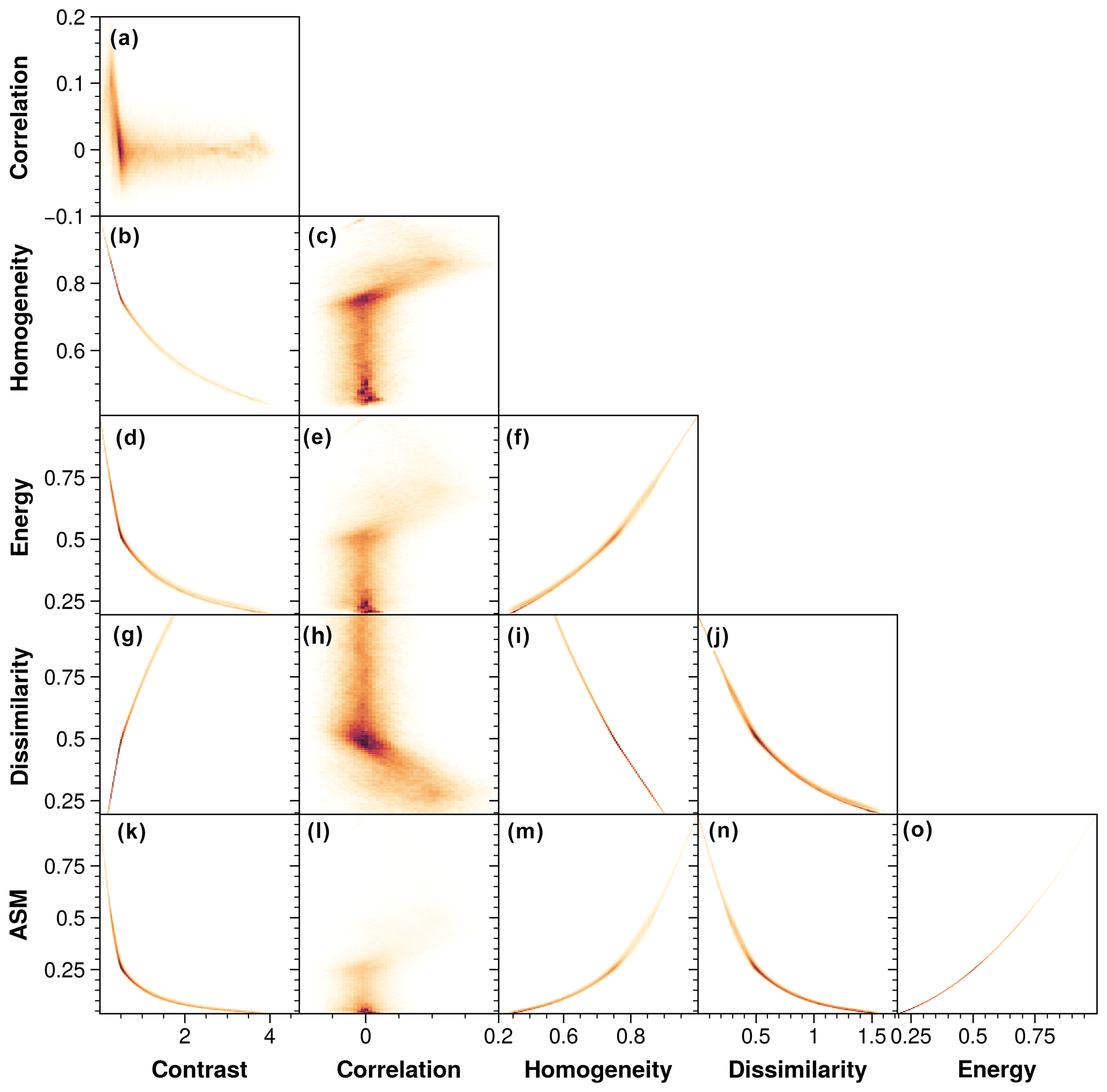
Figure 5 Density scatterplots across the six selected mean Haralick features for the structured-noise synthetic dataset.

In Fig. 5, we explored the relationships between the six chosen Haralick features by showing density scatterplots across each Haralick feature for the synthetic data. Strong exponential or squared relations exist between contrast, homogeneity, energy, dissimilarity, and angular second moment (ASM), while the correlation feature does not show any consistent pattern with any of the other features. This led us to retain only contrast and correlation as other features will be redundant with the contrast feature.

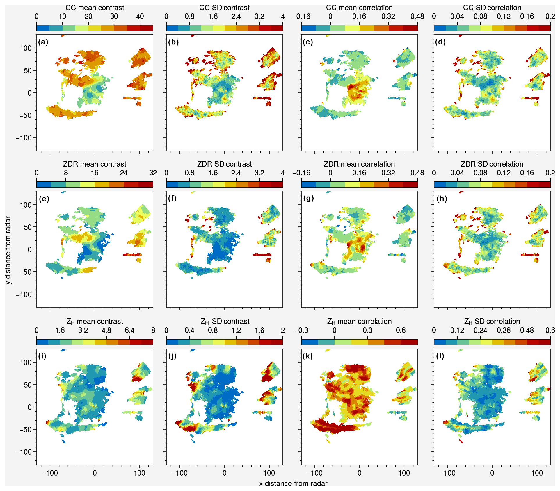
Figure 6 Mean and standard deviation of GLCM contrast and correlation calculated from the eight combinations of angles (θ = 0, $\mathit{\pi }/\mathrm{4}$, $\mathit{\pi }/\mathrm{2}$, $\mathrm{3}\mathit{\pi }/\mathrm{4}$) and distances (d = 1, 2). Data are from the S-band radar of Terrey Hills (Sydney) for 29 November 2019 at 05:07 UTC.

To explore the spatial distribution of contrast and correlation for various radar moments (ρ_HV, Z_DR, and Z_H), we selected the same event from the 2019/20 Australian Black Summer bushfires as shown in Fig. 1, where pyrometeors, clear air, and sea clutter can be observed within the same PPI. Notably, in Fig. 6a, the ρ_HV contrast is highest for the sea clutter and the pyrometeors, showing a strong potential to discriminate these two echoes from clear air using this feature. The standard deviation of the ρ_HV contrast (Fig. 6b) is highest at the edges of pyrometeors' plumes and sea clutter: this can be explained by the edge effects, where a smaller number of pixels are used to derive the GLCM, therefore providing larger directional variations from one (d,θ) combination to the next. The ρ_HV mean correlation (Fig. 6c) is higher for clear air than for the pyrometeors and sea clutter, providing here again another means of discriminating the two echoes from clear air. Local maxima of ρ_HV SD correlation can also be observed on the edges of the pyrometeors and sea clutter (Fig. 6d). Conversely, the values of mean contrast of Z_DR are not as high as ρ_HV contrast for pyrometeors, and some variability within the pyrometeors' plume can be observed with lower values of the Z_DR contrast closer to the fire area (Fig. 6e). On the other hand, the contrast of Z_DR for sea clutter shows consistently high values apart from the region located the furthest to the north. Both Z_DR and ρ_HV present high values of the mean correlation (Fig. 6g). Here again, standard deviations of contrast and correlation of Z_DR show local maxima (Fig. 6f and h), illustrating edges of objects and therefore less reliability regarding the mean features as compared to areas further away from the edges. The retrievals of Z_H contrast and correlation are shown in Fig. 6i and j, but no feature of particular interest was identified in these that could help segment the different echoes.

3.3 GMM training and labelling

Two days of S-band weather radar data from Sydney (Terrey Hills) were selected from the 2019/20 Black Summer season to build a dataset to train the GMM. The Sydney radar has a beam width of 1^∘ and a gate resolution of 250 m. All weather data used in this study are from the second tilt at 0.9^∘ elevation to minimise the introduction of ground clutter into the observations, despite its careful removal in the processing chain. These events were chosen so that the data contain a wide variety of clear-air, pyrometeor, sea clutter, and precipitation echoes, as discussed previously. For the selected period, this dataset contains over 4 500 000 data points. Based on the two criteria (AIC and BIC), an optimum value of k=5 was found, and while AIC and BIC continued to decrease for higher values of k, the magnitude of the drop was much lower, and their values plateaued beyond k=5 (not shown). Once trained, the model was applied to these data from two dates to qualitatively assess the classification and attribute to each cluster their respective object attribute (pyrometeors, clear air, sea clutter, or precipitation).

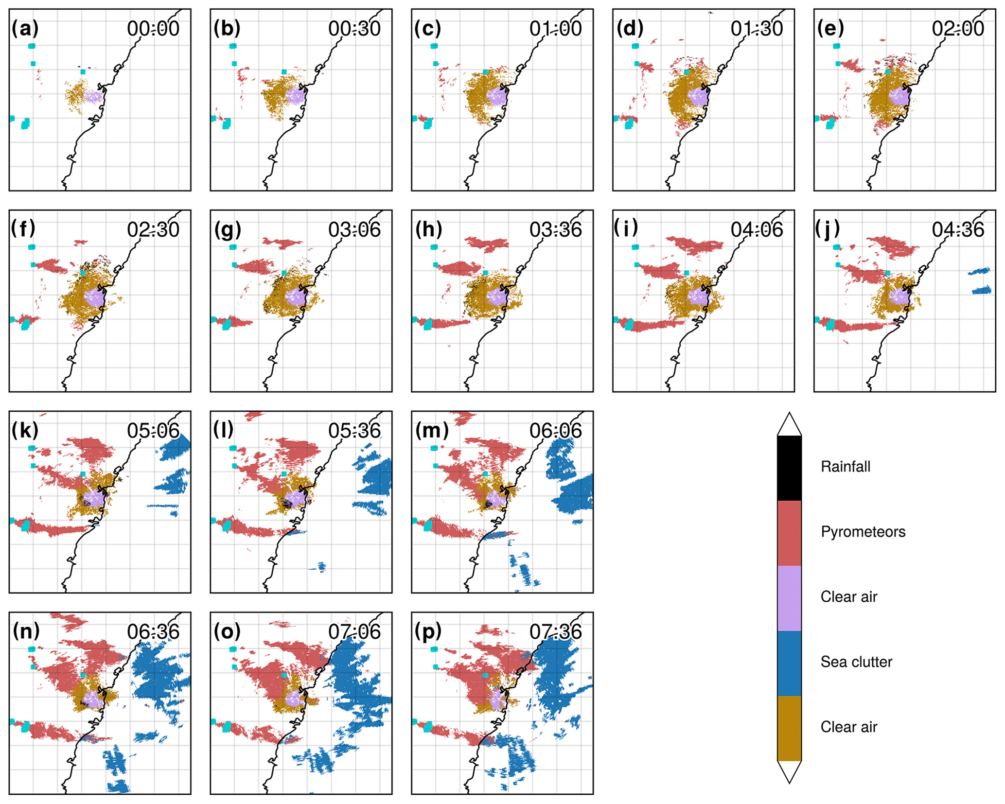
Figure 7 (a–p) Time series of segmented PPIs (second tilt at 0.9^∘ elevation) from the S-band Terrey Hills radar for 29 November 2019; Hotspots (for fire radiative power > 100 MW) derived from MODIS (sourced from FIRMS; Giglio et al. 2016; acquisition time 04:29 UTC) are plotted in dark turquoise. The time zone is UTC.

Figure 8 Spider plot showing the means across each feature of the Gaussian mixture model.

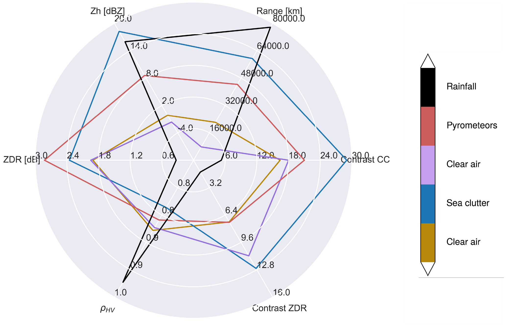
In Fig. 7a–p, each panel shows a timestamp of radar PPIs with the GMM-classified fields at 30 min intervals to assess the temporal continuity of the classification and discuss the interesting temporal evolution of the case. Clear air is distinguishable around the radar location and within a large radius (purple and gold colours), while three pyrometeors' plumes (in red) are visible to the west of the radar, progressively increasing in area as time progresses. The radar bins corresponding to pyrometeors' plumes are labelled as such in the very first frame, showing that only a dozen pixels are sufficient for the clustering algorithm to assign the label. Increasing areas of sea clutter (in blue) due to increasing anomalous propagation are visible to the east of the radar over the ocean starting in Fig. 7j and covering a half of the ocean within the frame in Fig. 7p. The labelling here performs well, with only a few points mislabelled as pyrometeors over the ocean for the large sea clutter object, except in Fig. 7l, m, and p, where the elongated southern pyrometeors' plume is mislabelled as sea clutter in some parts over the ocean. This concerns only a fraction of the total pyrometeors' plume areas, and in Fig. 7p, it is directly adjacent to the sea clutter, and therefore it is a complex scenario for the clustering algorithm to distinguish the two. Figure 8 provides some insight into each cluster's characteristics, by showing the mean across each variable of the GMM. Clear-air (purple and gold) means correspond to the lowest reflectivity values, lower values of the range, slightly positive values of Z_DR (around 2 dB), high values of ρ_HV (0.85), and low values of ρ_HV contrast. The distinction between the two clusters is for Z_DR contrast, with higher values of Z_DR contrast for the purple cluster. Without additional observations, we cannot evaluate whether this is due to a range bias or due to physical properties of the echoes. The pyrometeors' plume cluster presents on average higher values of Z_H than clear air, usually present at longer range (although as we can see in Fig. 5, this is not necessarily the case); the largest values of Z_DR (with a mean at 2.8 dB); relatively low ρ_HV (0.83); and relatively low Z_DR contrast (similar to clear air) but higher ρ_HV contrast (mean around 20). Finally, sea clutter shows a strong signature in both ρ_HV contrast and Z_DR contrast, with higher mean values of Z_H and range, relatively low values of ρ_HV, and relatively high values of Z_DR (2.4 dB).

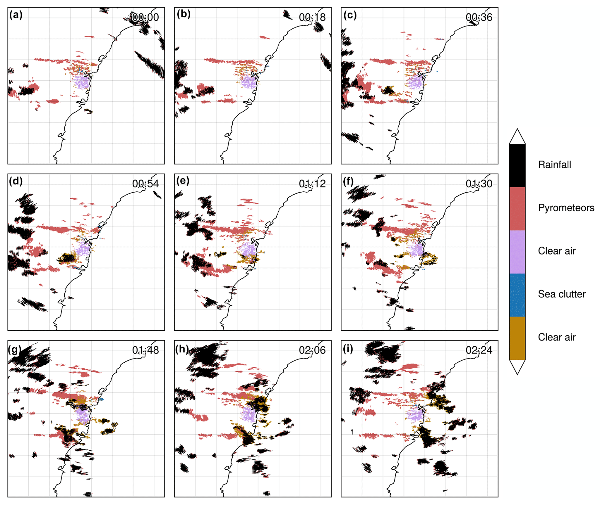
Figure 9 Time series of segmented PPIs (second tilt at 0.9^∘ elevation) from the S-band Terrey Hills radar for 2 December 2019, including the passage of showers over fire grounds and pyrometeors' plumes. 7. The MODIS overpass prior or concomitant to the radar observations did not detect hotspots because of total cloud cover over that period. The time zone is UTC.

To explore the capability of the algorithm to distinguish precipitation echoes, we applied the GMM retrieval to the training day with isolated showers (Fig. 9a–i). On that day, a very thin and elongated pyrometeors' plume is present to the northwest of the radar location, with another smaller plume to the southwest and a smaller pyrometeors' plume to the north of the radar. Scattered precipitation can be observed as a system moves eastwards. Overall, the precipitation object appears to be correctly labelled by the GMM, except for isolated pyrometeors' bins within some precipitation cells, as seen in Fig. 9d or e. Some complex interactions between clear air, pyrometeors' plumes, and precipitation can be observed in Fig. 9g and h, and therefore it is difficult here to quantify the performance of the classification. It is likely that some pyrometeors are entrained within the easterly flow, providing cloud condensation nuclei for droplets to form, while the clear air is also disturbed with the showers moving through. Overall, the classification effectively discriminates the major objects that are the main pyrometeors' plumes from precipitation showers and clear air. Based on the literature (McCarthy et al., 2018) and the location of the fire source, we can visually discriminate the echoes from the scene to support that validation. The precipitation cluster (Fig. 9) is characterised by very high ρ_HV, low Z_DR (just above 1), very low ρ_HV contrast (as expected since ρ_HV is close to unity for precipitation), and low Z_DR contrast.

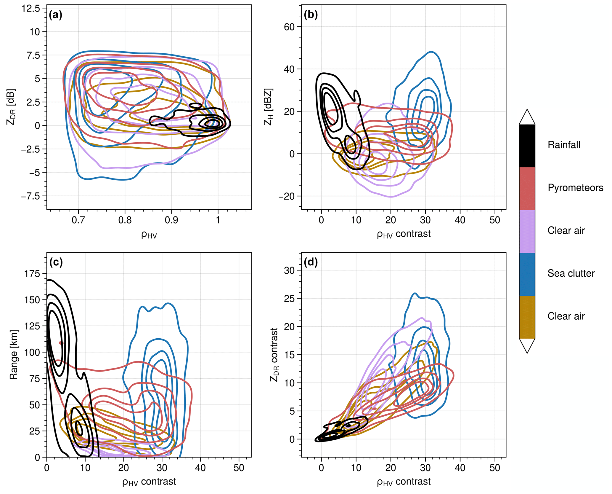
Figure 10 Joint distributions using kernel density estimation showing the distribution of values for each member of the GMM clusters for the training dataset. A randomly sampled subset (20 %) of the training dataset was used for plotting.

In Fig. 10, the cluster features are presented as joint distributions using kernel density estimation plots with the ρ_HV contrast as the x axis for Fig. 10b–d because this is one of the most discriminant characteristics as we have seen previously from Fig. 9. As described in the Introduction, Z_DR and ρ_HV clearly overlap for clear air, pyrometeors, and sea clutter, and these variables cannot solely be used to classify the different echoes. Only the precipitation cluster is well separated from the other clusters with high values of ρ_HV and Z_DR values just above zero. In Fig. 10b, the ρ_HV contrast clearly discriminates clear air from sea clutter and pyrometeors. The probability density estimates show distinct distributions for clear air and sea clutter, while the pyrometeors' distribution spans over a wider range of values. Z_H (Fig. 10b) and range (Fig. 10c) present similar discrimination potential, where clear air at shorter range from the radar is often associated with lower values of reflectivity (also an effect of the radar sensitivity, which is a function of range, so that clear air cannot be observed at long range), while sea clutter is often further away from the radar and essentially shows higher values of Z_H. However, this discrimination is not systematic as a strong overlap can be seen across all clusters for both range and Z_H, showing that while these features complement the texture fields, they certainly will not be sufficient to provide an effective classification. Finally, the contrast of Z_DR shows some distinction between clear air, pyrometeors, and sea clutter but with some overlap. The contrast of Z_DR only is not enough to provide a good discriminant but can be used to complement the ρ_HV contrast. Overall, the ρ_HV contrast appears to be the most effective feature to classify the various echo types, with support from the other complementary fields.

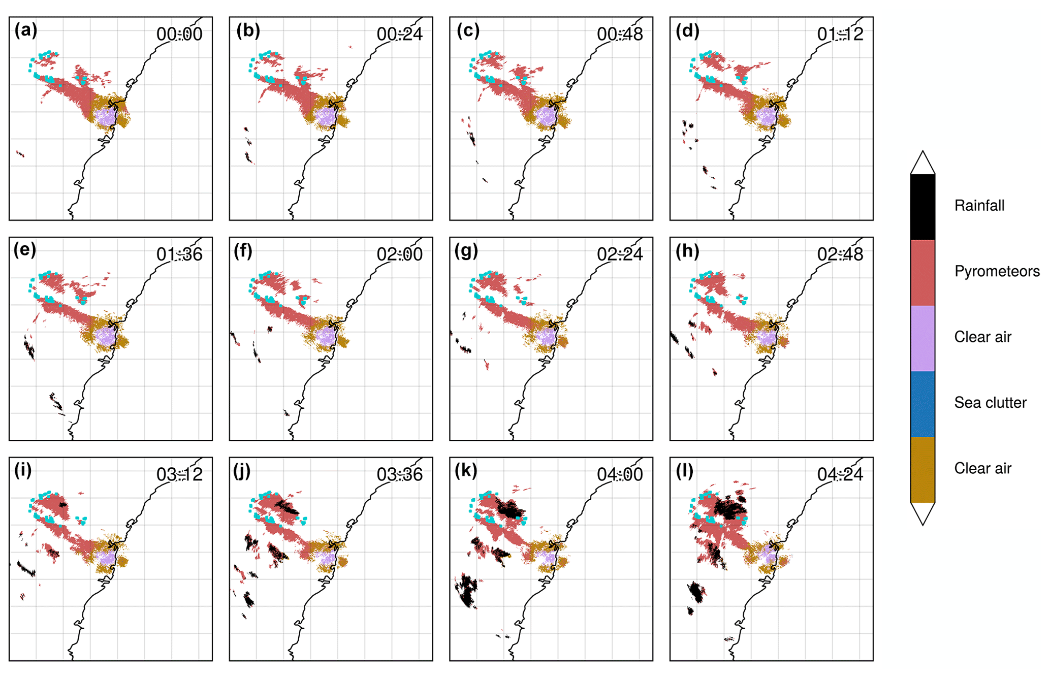
Figure 11 Time series of segmented PPIs (second tilt at 0.9^∘ elevation) from the S-band Terrey Hills radar for 22 November 2019. A pyroCb cloud was formed around 03:12 UTC as confirmed by satellite imagery (Himawari-8) of cloud top height. Hotspots (for fire radiative power > 100 MW) derived from MODIS (sourced from FIRMS; Giglio et al. 2016; acquisition time 00:06 UTC) are plotted in dark turquoise. The time zone is UTC.

3.4 Evaluation using an independent radar dataset

While the satisfactory performance of the classifier was demonstrated for cases that were used to train the model, it is necessary to also evaluate the model on data that have not been used for training. The date of 11 November 2019 was selected since this day featured a pyrometeors' plume moving in the direction of the radar, with consistent clear-air echoes through the observation period, and the initiation of a pyroCb cloud later in the day. In Fig. 11a–h, two main pyrometeors' plumes are clearly identified, with the largest being in contact with the clear air. While the exact boundary between clear air and pyrometeors cannot be verified with auxiliary data, it is reasonable to assume that the boundary of the two objects is well defined (clear air and pyrometeors' plume). At 03:12 UTC (Fig. 11i), precipitation can be seen within the pyrometeors' plume, and this area increases in size in the next four frames. This corresponds to the formation of the pyroCb (as seen in the brightness temperature on Himawari-8, not shown) and precipitation in the lower levels: the PPI shown in Fig. 11 corresponds to the tilt at 0.9^∘ elevation; therefore the northernmost precipitation cluster in Fig. 11i–l is observed at 110 km from the radar location, i.e. a corresponding altitude above ground level of 2.2 km. This validation demonstrates the robustness of the method when trained for days that include a variety of echoes. The possibility of transferring that trained model to radars with other characteristics (beam width, sensitivity, resolution, calibration) will require a dedicated study.

4 Discussion and conclusions

In this study, we have demonstrated that statistical texture can be retrieved directly from weather radar data in spherical coordinates using an adapted approach based on gray-level co-occurrence matrices. The use of a varying window width (along the axis perpendicular to the range axis) enabled us to mitigate a range-dependent bias in calculated texture fields, an issue documented by other authors (Gourley et al., 2007; Stepanian et al., 2016). We believe that this bias has limited the wider use of spatial texture applied to weather radar data to date. For weather radar variables with local spatial variability fields such as ρ_HV and Z_DR, the use of GLCMs on interpolated gridded data is not suitable as interpolation will smooth the fields and strongly affect the retrieved texture. Therefore, it is essential to retain information in polar coordinates, further motivating the need for the varying-window-width approach. However, our approach only indirectly accounts for relations between resolution of observations and the scale of the observed object, a well-known effect in remote sensing application originally described by Woodcock and Strahler in 1987. For example, vortices that have a typical scale of a few hundred metres can be partially resolved at close distance to the radar but will be lumped at long range along the perpendicular axis to the range axis. Calculating the texture along a much wider window at close range enables us to increase the number of data points used to calculate the GLCM, effectively reducing the effect of local extrema and smoothing the retrieved texture field. The results obtained for synthetic spatially structured random noise show that the varying-window approach enables the retention of both the spatial organisation of the fields and their absolute values. Texture features such as contrast for synthetic data show the same minima and maxima at both close and long range, which is not the case when a fixed window is used. Finally, since neither spectrum width nor radial velocity has been used in the classification, these two radar variables can be interpreted independently to provide insights into the turbulent features of pyrometeors' plumes.

A limitation in validating our echo classification is the lack of a reference classification. We can only qualitatively assess the accuracy of the results based on extra knowledge such as the areas of actively spreading fire, consistency in the time series, climatological presence, location of sea clutter for the specific radar, and diurnal evolution of clear-air returns. Based on this additional information and the dual-polarised moments, a trained radar expert would be able to manually classify echoes in the complex scene shown in Fig. 2 and likely achieve a similar result to our texture and GMM approach. However, a human manual classification would fail to define interfaces between clear air and pyrometeors where the boundaries are blurred. From this perspective, we believe that our results are at least as skilful as those of an expert and, in some cases, likely less biased because of their objectivity. There are instances when pyrometeors and biological echoes will mix, and for a given bin, radar echoes would thus be a mixture of both. Because we only used the second (0.9^∘) tilts in this paper, we minimised the potential occurrences of shallow diluted pyrometeors' plumes where biological echoes could dominate over pyrometeors. We did not evaluate our approach against other proposed approaches such as that of Zrnic et al. (2020) as it is well known that a fuzzy-logic-based approach would need a priori information on the distribution of the polarimetric variables; therefore it would provide a biased result and no reference result with which to compare. Zrnic et al. (2020) indeed showed that biological echoes (insects/birds) and pyrometeors' echoes overlap and that they observe misclassification with their fuzzy-logic algorithm. The main advantage of this newly automated classification is that it provides identification of pyrometeors, providing the foundations to further apply other algorithms. There remain some issues that could see improvements or at least can be flagged with a degree of uncertainty in the retrievals. However, in cases where only a few data points are available to calculate texture, such as for isolated pixel groups or the extremities of pyrometeors' plumes, the retrieved texture fields will show large standard deviations across the distance–angle combinations. This variability is present due to the small sample size and can result in potentially unrealistic values of the mean texture retrievals. Another ongoing issue is the mislabelling of data points located over land as sea clutter. These data points are primarily located within pyrometeors' plumes, and this mislabelling occurs due to the somewhat similar textural properties of pyrometeors and sea clutter. Our correction using a land–sea mask enabled us to address this issue in a straightforward manner. Notably, only a very small number of data points are mislabelled as pyrometeors over the sea (in areas where we know these are sea clutter echoes and not pyrometeors' echoes). Finally, a greater diversity of echoes in the training dataset could be considered, and the inclusion of frozen precipitation such as hail and snow echoes would allow for the capture of the full diversity of echoes that can be encountered in the vicinity of the Terrey Hills radar. This would necessitate increasing and optimising the k value in the GMM.

We currently see two main limitations to a generalisation and a wider use of our approach. Firstly, texture fields are dependent on several factors such as radar characteristics, including frequency, resolution, sensitivity, calibration, and accuracy. Typically, absolute values of radar moments will be affected by the sensitivity, calibration, and accuracy of the radar and, in turn, the spatial field of these moments, and its distributions could be seeing extreme values or outliers, skewed distributions of values, or wider or narrower widths of their distributions. Since the GLCMs are affected by spatial differences between values, an increase or decrease in these differences would affect the texture fields. The number of samples collected on each ray will also affect the texture due to sampling variability. The radar resolution will also be an important factor affecting the texture because of the averaging of inter-bin variations in radar variables for coarse resolutions, as opposed to a higher bin-to-bin contrast for higher resolutions. Typically, for various resolutions of the observations and a given size of the observed object (typically vortices of hundreds of metres), the resulting variable fields would see lumped values at coarse resolution, where higher resolution would resolve the object, and see strong bin-to-bin variations. Finally, the radar frequency would also affect the texture field, as for the same scene observed by X- or S-band radars, one would see more attenuation at the X-band and different thresholds of detection for ash-sized particles for example, resulting in different radar variable fields. This frequency effect is, however, expected to be minimal compared to the ones described above. Typically, the systematic error in Z_DR for pyrometeors is expected to be larger than that for rain or other echoes. The effect of scale as discussed previously and the relation between the observed object and the resolution of the observation will greatly influence textural retrievals. Of particular interest are texture retrievals from portable weather radar observations (McCarthy et al., 2018, 2017) at X- or Ka-bands that are deployed around wildfires and provide unique insights into wildfire plume dynamics and composition. Systematic retrievals of texture fields, in particular the contrast of the correlation coefficient for such observations, could help interpret these high-resolution datasets by identifying areas or volumes with predominantly similar echoes or a large diversity of echoes. The absolute values of texture fields are also dependent on the chosen quantisation (rescaling from a variable range to a chosen range of gray scale levels). Addressing this issue should be straightforward following the approach proposed by Löfstedt et al. (2019). Secondly, the computational efficiency of texture calculations is a significant issue for operational use. The current implementation requires 3 min of CPU time (on an ARM-based Apple M1 CPU) to retrieve texture fields from three radar moments for two Haralick features and for eight combinations of distances–angles. This is a well-known limitation of GLCMs (Clausi and Jernigan, 1998), but there are multiple avenues to reduce this computational cost. Initial work exploring the vectorisation of the GLCM implementation, as opposed to nested loops, could reduce computational cost by a factor of 5, and masking regions with no data could also drastically reduce the cost by a factor of 10. Finally, parallelisation of the GLCM using GPUs can reduce the computational cost by several orders of magnitude, with early testing indicating that the processing time is reduced from 3 min to approximately 10 ms.

The method presented here represents a significant step towards temporal and spatial insights into fire–atmosphere interactions where previously pyrometeor returns have largely been grouped with a broader “non-meteorological” class of returns. While there have been a number of studies that leverage the highly detailed information available from radar to develop insights into plume development above wildfires, and even into wildfire behaviour, they have been restricted to case-study-level analyses (McCarthy et al., 2019). This has principally been due to lack of automated assessment of pyrometeor returns, necessitating manual interpretation and classification, whereas automated hydrometeor classification is well advanced due to a significant body of research. The possibility of automatically assessing physical processes, from a statistical point of view, over multi-day and multi-week fire campaigns, as well as between different fires, will be significant for the fire science discipline. The discussed method will allow temporal examination of fire escalation, area growth, and fuel consumption rates as suggested by Duff et al. (2018) while being able to be specific about the type (shape, size, permittivity, concentration) of pyrometeors and the presence of deep and moist convection coupled to fires based on the radar data alone.