A physically based correction for stray light in Brewer spectrophotometer data analysis

Brewer ozone spectrophotometers have become an integral part of the global ground-based ozone monitoring network collecting data since the early 1980s. The double-monochromator Brewer version (MkIII) was introduced in 1992. With the Brewer hardware being so robust, both single- and double-monochromator instruments are still in use. The main difference between the single Brewers and the double Brewers is the much lower stray light in the double instrument. Laser scans estimate the rejection level of the single Brewers to be 10^−4.5, while the doubles improve this to 10⁻⁸, virtually eliminating the effects of stray light. For a typical single-monochromator Brewer, stray light leads to an underestimation of ozone of approximately 1 % at 1000 DU ozone slant column density (SCD) and can exceed 5 % at 2000 DU, while underestimation of sulfur dioxide reaches 30 DU when no sulfur dioxide is present. This is because even a small additional stray light contribution at shorter wavelengths significantly reduces the calculated SCD at large values. An algorithm for stray light correction based on the physics of the instrument response to stray light (PHYCS) has been developed. The simple assumption is that count rates measured at any wavelength have a contribution from stray light from longer, and thus brighter, wavelengths because of the ozone cross-section gradient leading to a rapid change in intensity as a function of wavelength. Using the longest measured wavelength (320 nm) as a proxy for the overall brightness provides an estimate of this contribution. The sole parameter, on the order of 0.2 % to 0.6 %, that describes the percentage of light at the longest wavelength to be subtracted from all channels is determined by comparing ozone calculations from single- and double-monochromator Brewers making measurements side-by-side. Removing this additional count rate from the signal mathematically before deriving ozone corrects for the extra photons scattering within the instrument that produce the stray light effect. Analyzing historical data from co-located single- and double-monochromator Brewers provides an estimate of how the stray light contribution changes over time in an instrument. The corrected count rates of the measured wavelengths can also be used to improve other calculations: the sulfur dioxide column and the aerosol optical depth, the effective temperature of the ozone layer, or any other products. A multi-platform implementation of PHYCS, rmstray, to correct the count rates for stray light and save the corrected values in a new B-file for use with any existing Brewer data analysis software is available to the global Brewer user community at https://doi.org/10.5281/zenodo.8097038 (Savastiouk and Diémoz, 2023).

1 Introduction

Developed in the late 1970s at what is now known as Environment and Climate Change Canada (ECCC), the Brewer spectrophotometer has become an important research and monitoring ground-based instrument to determine, among other quantities, the amount of ozone in the atmosphere and the solar ultraviolet (UV) irradiance reaching the surface (Kerr et al., 1985). As an essential component of the World Meteorological Organization Global Atmosphere Watch (WMO-GAW) O₃ observing system, the Brewer network, which today consists of more than 200 operating instruments, contributes with its long-term data set to understanding the chemistry and dynamics of the Earth's atmosphere, as well as their variations due to anthropogenic emissions and climate change (Eleftheratos et al., 2022; WMO, 2022; Petkov et al., 2023).

The first Brewers were conceived as single-monochromator spectrometers; i.e., they were equipped with only one dispersion element to separate sunlight into a range of individual wavelengths to be analyzed. Double-monochromator Brewers were introduced only in the 1990s to achieve better spectral purity, thus reducing the so-called internal spectral (or out-of-band) stray light. The latter is defined as the fraction of radiation with wavelengths other than the one being measured and yet able to reach the detector due to scatter inside the instrument. Spectral stray light is not specific to the Brewer spectrophotometer but is present in any single-monochromator system, including new-generation instruments based on array detectors (Zong et al., 2006). Indeed, the problem is actually worse for array detectors because of the much larger solid angle within the instrument that contributes to the signals measured. There are other types of stray light, e.g., originating from the scattering of sky light entering the instrument field of view or from ineffective filtering of polarized light, but they are not addressed in the present study.

Due to the strong irradiance gradient in the UV-B (wavelength range 280–315 nm) band of the solar spectrum, spectral stray light makes irradiance at shorter wavelengths seem significantly higher than it actually is because of photons with longer wavelengths being detected when observing short wavelengths. This instrumental artifact leads to an overestimation of the global irradiance in the UV-B (Lantz et al., 2002) and underestimation of total ozone and sulfur dioxide (e.g., Redondas et al., 2014). Other retrieved quantities, such as the ozone profile (Petropavlovskikh et al., 2011) or the aerosol optical depth (AOD; Arola and Koskela, 2004; Silva and Kirchhoff, 2004; Hrabčák, 2018; López-Solano et al., 2018), may be affected as well. The contribution to the measured radiation from stray light is generally small in an absolute sense; however as the amount of ozone in the optical path, and thus the absorption, increases, the light at short wavelengths dims, while stray light stays relatively bright. This is especially true for measurements at large solar zenith angles at times close to sunrise and sunset or at high latitudes, where the slant column density (SCD, i.e., air mass times the vertical column) of ozone is large most of the year due to both solar elevation and ozone climatology. However, stray light may complicate ozone calculations even in midlatitudes in the winter (Stübi et al., 2017).

With the Brewer hardware being so robust, both the single-monochromator and the double-monochromator instruments are still in use. Therefore, to make retrievals from single Brewers comparable to double Brewers, the effect of spectral stray light must be thoroughly characterized and corrected. Only then can the global ozone data set be homogenized to allow an accurate determination of long-term trends or the validation of estimates made from space.

Several studies have addressed the effect of stray light on Brewer retrievals and proposed some solutions going beyond the mere cutting off the measurements at large solar zenith angles (Stübi et al., 2017). These algorithms often rely on complex parameterizations to correct the calculated ozone vertical column density (VCD) as a function of the optical path through the atmosphere (Karppinen et al., 2015; Redondas et al., 2018; Vaziri Zanjani et al., 2019). Only a few authors proposed methods making direct use of the light detected by the Brewer. Kerr (2002), for example, derived the stray light spectrum based on actual measurements; however, the methodology relies on a non-standard (group-scan) routine and on a specific (laser-based) instrumental characterization not usually available, making this method impractical for the entire Brewer network. Hrabčák (2018) derived an approximate estimate of the stray light effect from global UV measurements on cloudless days and then parameterized it as a polynomial function of the solar zenith angle to provide more accurate AOD values.

This study presents a much simpler algorithm (PHYsically based Correction for Stray light, PHYCS, pronounced as “fix”) to make the Brewer retrievals of total ozone and sulfur dioxide virtually unaffected by stray light. The effect on global UV irradiance measurements is not addressed here. The algorithm is based on reversing the stray light effect mathematically by subtracting its contribution from the detected count rates before calculations for any products are done. PHYCS only needs the calibration of one parameter for ozone and one for sulfur dioxide, without requiring additional instrumental characterizations or complex parameterizations. This method has several advantages:

• It only uses the count rates detected by the Brewer to estimate and remove the stray light contribution. Hence, the effects of the instrument characteristics are fully separated from the effects of the environmental conditions so that the algorithm can be applied as it is to any observation geometry.

• The algorithm has been implemented in a multi-platform software package. The latter corrects the count rates in the original data files; thus it allows the operators to keep using any existing Brewer data processing tools for the constituent retrievals.

• It can readily become part of the calibration process during regular on-site audits with travelling standards, provided that the latter ones are already characterized for the stray light effect.

The present paper is organized as follows. Section 2 introduces PHYCS and its general principles. Section 3 presents the results of radiative transfer calculations, confirming the assumptions which are at the basis of the algorithm, and an application to the analysis of real data. A discussion about the implications for the Brewer calibration and data processing follows (Sect. 4). Conclusions and perspectives complete the article (Sect. 5).

2 Data and methods

2.1 Instruments and data

The Brewer spectrophotometer and the standard data processing algorithm are described in numerous publications (see, for example, Siani et al., 2018, Zhao et al., 2021, and references therein). In Appendix A, we provide a basic background only as needed for this paper.

To show that PHYCS works well under different atmospheric conditions, data from the following Brewers at three locations were analyzed:

• The first location is Mauna Loa Observatory (MLO) in Hawaii, USA, hosting Brewers #009 and #119. This station is a pristine, premium site for Langley calibrations, located in the tropics at high elevation. Low total ozone and little ozone variability in the seasons are expected at this location. The instruments, belonging to ECCC, are operated jointly by the National Oceanic and Atmospheric Administration (NOAA) and ECCC.

• The second location is Toronto, Ontario, Canada, hosting Brewers #008 and #145. The station is in an urban environment located at midlatitude at low elevation. Moreover, the Toronto station is also home for the world Brewer reference (Zhao et al., 2021). The instruments are operated by ECCC.

• The third location is Alert, Nunavut, Canada, hosting Brewers #029 and #246. The station is located on the coast of an island surrounded by ice all year round, in a high-latitude environment. Alert is thus characterized by high variability in ozone VCD throughout the year. The range of the available solar elevation angles is limited owing to the high latitude of the site. The Brewers are operated by ECCC.

More details are provided in Table 1. The choice of the instruments is based on the fact that each of these stations has at least one double-monochromator Brewer version (MkIII) and at least one single Brewer (MkII, MkIV or MkV) that operated continuously for at least 6 months (to explore the entire range of the solar zenith angles at each location). Data from all the above instruments in the interval covering the 6 months from 22 December 2019 to 22 June 2020 were analyzed.

Table 1 Brewer spectrophotometers employed in this study.

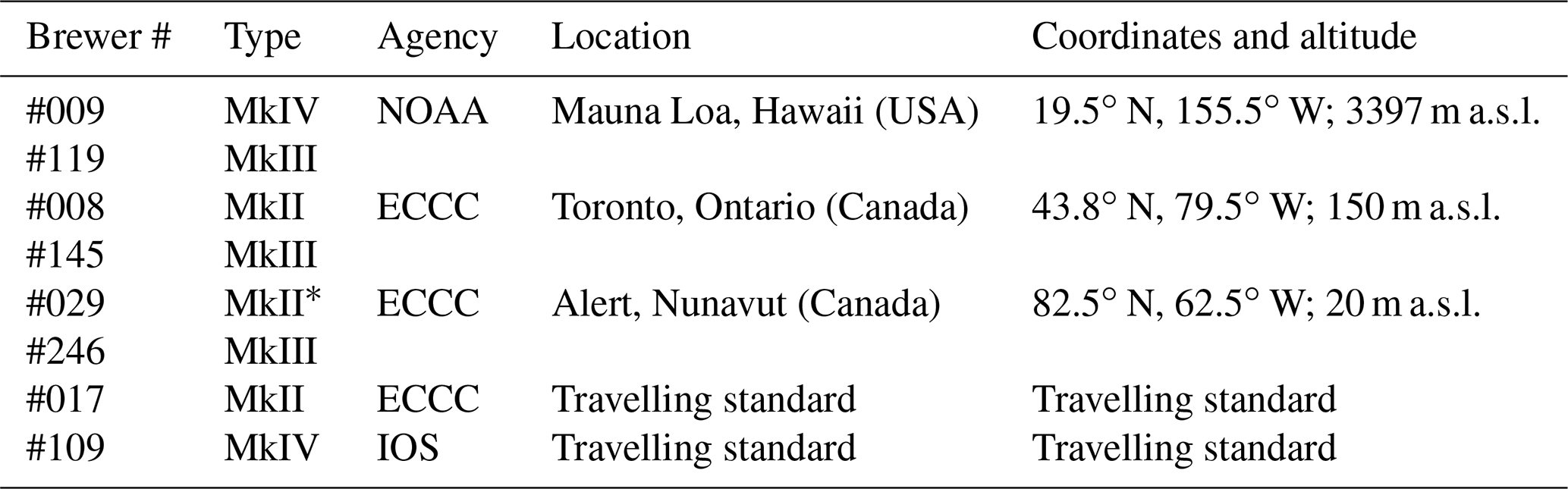
^* Brewer #029 is actually a MkV, i.e., a Brewer with a modified filter wheel to be able to switch from UV to visible. However, this is not relevant for the present study.

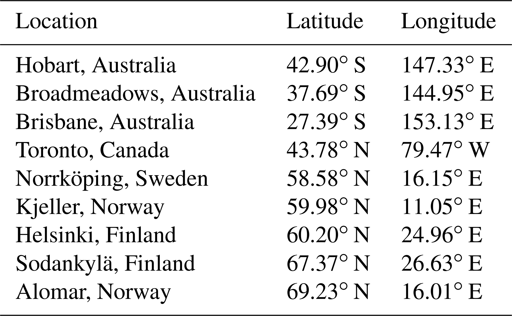
Additionally, the data from the travelling standard Brewers #017 and #109, operated by International Ozone Services, Inc. (IOS), were also analyzed. The former instrument allows us to assess the long-term changes in the stray light effect. Indeed, for this spectrophotometer the record from 1993, when the double-monochromator Brewers were first introduced, to 2021 was considered. Additionally, data collected by Brewer #109 in 2022 at several stations were used to test PHYCS under different conditions. In recent years Brewer #017 has travelled mostly to central Europe, and the IOS standard #109 has visited nine stations in 2022 in both the Northern Hemisphere and Southern Hemisphere with vastly different observing conditions (Table 2). The data from all these sites were processed with a single set of stray light correction factors to confirm that these coefficients only depend on the instrumental characteristics, not on the location (Sect. 3.2.4).

Table 2 Stations visited by the travelling standard Brewer #109 in 2022 and employed in this study to test PHYCS under different conditions.

Finally, to study the stray light effect with radiative transfer simulations (Appendix B2), a set of laser scans measured by the ECCC personnel in the early 2000s (Fig. 1) were employed. These spectra were obtained for several Brewers by scanning the 325.029 nm emission line of a helium–cadmium (HeCd) laser.

2.2 Stray light definition, phenomenology and proposed reversal algorithm

When measuring radiation at wavelength λ by means of a spectrometer with slit width δλ, the stray light is defined as radiation of wavelengths outside the bandpass λ±δλ that reaches the detector.

The presence of stray light is attributed to scatter inside the instrument by impurities and imperfections in the optical elements (Woods et al., 1994). For example, the monochromator in Brewers is routinely opened for maintenance and dust can enter the instrument quite easily. Then, having bright light while measuring solar radiation contributes to both electro- and photophoresis, and dust accumulates on optical element surfaces, such as the spectrometer mirror (Kerr, 2002). This aging leads to an increase in the stray light effect with time. Holographic diffraction gratings are also a very important source of scattering inside the instrument, depending on their ruling density and line quality. Generally speaking, stray light is larger for gratings with lower line density (Kiedron et al., 2008). Hence, as a rule of thumb, the effect is more pronounced in MkIV Brewers than in MkII Brewers (see Appendix A1).

The difference in stray light among Brewer types is illustrated in Fig. 1, where the responses of several instruments to the quasi-monochromatic radiation emitted by a 325 nm laser are shown (Savastiouk and Wardle, 2007). The effect of the resolution of the instrument due to the finite dimensions of the slits can be noticed as a broadening of a few nanometers around the excitation wavelength (“core” region), while the effect of stray light manifests itself as a non-zero background irradiance at wavelengths far away (“shoulder” and “wing” regions). Although the level of stray light looks very low compared to the signal, even in single-monochromator instruments, its contribution integrated over the whole spectrum has a pronounced effect. The figure confirms that, with the exception of a few instruments, MkIV Brewers show larger stray light than MkII Brewers, and MkIII Brewers reject stray light about 10³ times better than single-monochromator Brewers. It is interesting to note that even Brewers of the same type exhibit some heterogeneity in their stray light levels, likely owing to different mechanical and optical characteristics, their age, and their state.

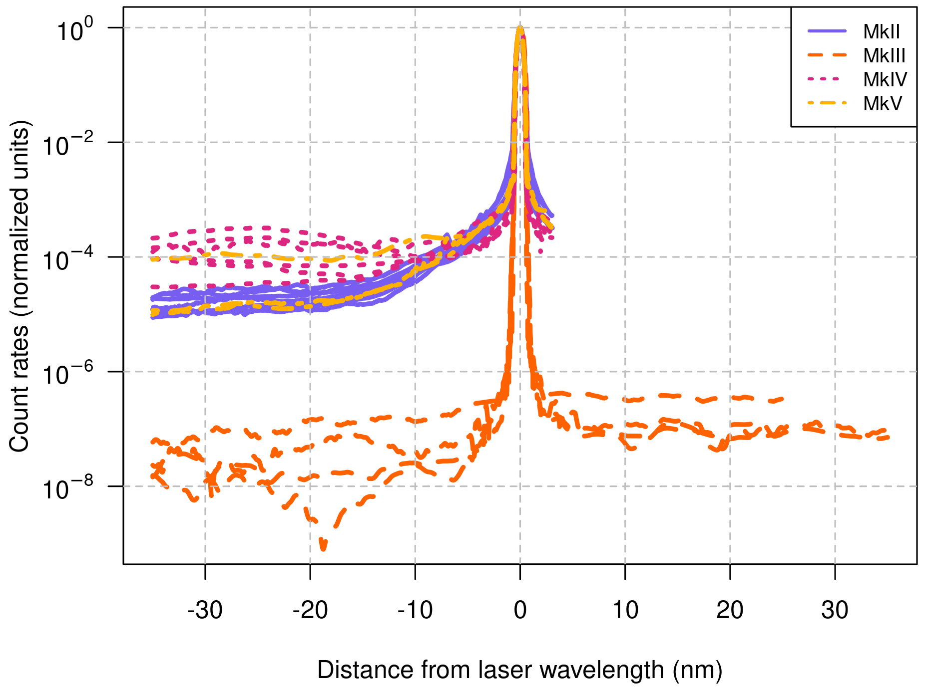
Figure 1 Spectra resulting from scanning a 325 nm laser line with different Brewers. The effect of stray light is clearly visible as an increase (in single-monochromator Brewers compared to double-monochromator Brewers) in the count rates at large distances from the excitation wavelength. The spectra were normalized to their respective peak values and coloured based on the Brewer type (MkII: serial numbers #012, #014, #015, #017, #033, #037, #053, #055, #113; MkIII: #021, #085, #107, #111, #128; MkIV: #007, #009, #071, #079, #080, #082, #084, #109; MkV: #029, #039, #042). Scans from single Brewers are incomplete towards larger wavelengths, owing to the reduced spectral range of these instruments, only up to 328 nm.

To parameterize the stray light and separate it from the “true” (unknown) irradiance, a formal framework is introduced, where the detected count rate, I_d, is represented as a sum of the true count rate, I_t, and the stray light count rate, I_s:

$$\begin{array}{}\text{(1)}& I_{\mathrm{d}}\left(\mathit{\lambda }\right)=I_{\mathrm{t}}\left(\mathit{\lambda }\right)+I_{\mathrm{s}}\left(\mathit{\lambda }\right).\end{array}$$

For a given wavelength, I_s(λ) depends on the instrumental characteristics and the intensity and shape of the solar spectrum. Among the wavelengths used in the Brewer observations, slit 5, nominally at 320 nm, is the least affected by the presence of ozone. Hence, the detected count rate at slit 5, I(320 nm), is used as a proxy for the level of light available for stray light. We can introduce a function (of the wavelength and presumably other parameters), f_s(λ,…), to have

$$\begin{array}{}\text{(2)}& I_{\mathrm{s}}\left(\mathit{\lambda }\right)=f_{\mathrm{s}}(\mathit{\lambda },\mathrm{\dots })I\left(\mathrm{320}\mathrm{nm}\right).\end{array}$$

Now, our working hypotheses are the following:

1. The stray light contribution I_s(λ) (and hence f_s(λ,…)) is only weakly wavelength-dependent in the narrow band used by the Brewer to retrieve ozone and sulfur dioxide (306–320 nm), and it adds light to all slits almost uniformly in the count rate space. The exact values of I_s and f_s make almost no difference to the bright light at longer wavelengths, but an accurate estimation of I_s at the shortest wavelengths is crucial for ozone and sulfur dioxide retrievals. To be precise, the calculations (Sect. 3.1) show that we can replace function f_s(λ) with two stray light coefficients, one (α) for slits 2–5 and another (β) for slit 1.

2. These coefficients do not change as a function of the atmospheric and observing conditions. This allows the determination of α and β through a calibration process (Sect. 2.3) and the use of them under any condition thereafter.

To support these hypotheses, stray light in Brewers was simulated numerically (Sects. 2.4 and 3.1).

Based on the assumptions above, Eq. (2) becomes

$$\begin{array}{}\text{(3)}& I_{\mathrm{t}}\left(\mathit{\lambda }\right)=\left\{\begin{array}{ll}{I}_{\mathrm{d}}\left(\mathit{\lambda }\right)-\mathit{\alpha }I\left(\mathrm{320}\mathrm{nm}\right)& \text{slits}\mathrm{2}-\mathrm{5};\\ I_{\mathrm{d}}\left(\mathit{\lambda }\right)-\mathit{\beta }I\left(\mathrm{320}\mathrm{nm}\right)& \text{slit}\mathrm{1},\end{array}\right.\end{array}$$

with I_t(λ) being the true count rate. Note that Eq. (3) is linear (in the “count rate space”). However, as soon as logarithms of the counts are considered while solving the Bouguer–Lambert–Beer law equation (Bouguer, 1729), the effect becomes highly non-linear. This is why most previously published research is focused on using a range of complicated non-linear functions for correcting the ozone values. In contrast, PHYCS addresses the core of the stray light effect and reverses it in the count rates.

From a practical perspective, to mathematically reverse the effect of the stray light in the Brewer data, the detected count rate at each slit is corrected for the dark counts and the dead time, and then the stray light contribution is removed using Eq. (3). Once the count rates at all slits have been corrected, the ozone and sulfur dioxide, as well as any other product, can be derived using the standard or custom algorithms. This also allows the user to apply PHYCS upstream of other corrections, e.g., to account for changes in the Brewer radiometric sensitivity (“standard lamp” correction).

2.3 Determination of stray light coefficients

PHYCS requires a calibration process to determine factors α and β. Three methods are discussed: the first one uses a reference Brewer that has no measurable stray light or has already been calibrated for the stray light correction algorithm (Sect. 2.3.1), the second method involves absolute calibration from Langley plot observations (Sect. 2.3.2), and the third method is based on a statistical analysis of a long-term data set (Sect. 2.3.3).

In most cases, the transfer method will be used in practice, since an absolute calibration can only be performed in a pristine environment with stable ozone, sulfur dioxide and aerosol conditions, and there are only a few locations in the world satisfying this requirement to the desired level of accuracy (Zhao et al., 2023).

2.3.1 Calibrating using a reference instrument

An iterative calibration process is employed to establish the coefficients α and β. Since the Brewer algorithm for sulfur dioxide uses total ozone column, it is important to first establish α and only then proceed with the calibration for β. Calibrations for α and β involve virtually identical steps, so only the process for α is described:

1. The calibration starts with first guesses for α and for the extra-terrestrial coefficient (ETC${}_{{\mathrm{O}}_{\mathrm{3}}}$; Appendix A3). α can be taken from model calculations (Sect. 3.1), and the first guess for ETC${}_{{\mathrm{O}}_{\mathrm{3}}}$ can be the one in use or calculated from the standard ozone calibration procedure for Brewers as described in Appendix A3. Depending on the observing conditions during the standard ozone calibration, that first guess is very likely an underestimate of the true ETC that should be used together with the stray light correction.

2. Both α and ETC are varied to have ozone calculations match those from the reference Brewer. This step is similar to the standard Brewer calibration, where only the ETC is varied to match the retrievals from the reference Brewer. Calculations (Sect. 3.1) show that the Brewer retrievals are sensitive to the values of α and ETC at different air mass factor (AMF) and ozone SCD ranges, which allows the two unknowns to be estimated independently. Any non-linear multi-parameter optimization algorithm can be employed for the purpose, even a simple trial-and-error method works well.

3. Unlike the standard ozone calibration, where the AMF is limited to the range of 1.2–3.2, the data from a wider range 1.2–4.5 are used, if available, since the stray light effect is more pronounced at larger slant ozone amounts. The direct-sun data at AMFs larger than 4.5 are affected by the Rayleigh and aerosol scattering in the field of view (Kerr, 2002; Arola and Koskela, 2004) and will not be considered here.

2.3.2 Calibrating using the Langley method

In the rare situation when a Brewer is at a location suitable for absolute calibration (Zhao et al., 2023), the Langley plots can be used to establish both α and the ETC without any additional reference instrument. This method also involves an iterative process but is simpler in calculations than the previous one since only one parameter, α, is varied to have the Langley fit as close to a straight line as possible. The residual from the fit can be used as the metric, as also done by Vaziri Zanjani et al. (2019). Then, the ETC is determined as the intercept of the Langley fit in the standard way. This method has, however, significantly higher demand for the quality and the quantity of the data and for the slant ozone range. First, all known instrumental corrections need to be applied (instrumental temperature, dead time, colour of the neutral density filters, etc.). Second, the physics of stratospheric ozone works against finding a solution in this situation: pristine locations for absolute calibrations are close to the Equator because that is where ozone is more stable. Those are also the locations where the total ozone column is lower, making it difficult to collect data at large ozone SCDs, needed for a reliable determination of α.

2.3.3 Monitoring the stability of the stray light coefficients with statistical methods

In places where single Brewers cannot be regularly compared to reference instruments with lower stray light, the user can rely on statistical methods to monitor the stability of the stray light correction. The method proposed here is based on plotting a large number of individual retrievals (ozone or sulfur dioxide) as deviations from their respective daily medians. If little or no systematic daily variations in ozone and sulfur dioxide are expected, then the differences from the daily medians should be almost randomly distributed around zero. Hence, any clear departure from zero increasing with ozone SCD could be a sign of the stray light effect. Similar techniques were used, for example, by Diémoz et al. (2015) and Stübi et al. (2017) to estimate the stray light effect on ozone retrievals.

This method is likely not precise enough to provide an absolute estimate of α and β but can be very useful to monitor the stray light effect on a continuous basis in the absence of a reference Brewer and to identify sudden variations indicating that the instrumental properties have changed and to recover data from a series which was not characterized for the stray light correction.

2.4 Radiative transfer simulations

Simulations are helpful to support the hypotheses at the base of our algorithm (Sect. 2.2) and to first test our correction in a controlled setting, e.g., with an a priori knowledge of the “true” vertical column density. Moreover, they allow us to check the consistency of PHYCS with the existing methods based on radiative transfer calculations (e.g., Kiedron et al., 2008; Karppinen et al., 2015; Vaziri Zanjani et al., 2019). As opposed to other studies, the radiative transfer results were not used to correct the Brewer count rates but were only employed to obtain a first guess of the stray light correction factors α and β.

Notably, this part of the study consists of three simulations (S1–S3) with different objectives.

• S1. We first simulate direct-sun Brewer measurements without stray light and perform standard O₃ and SO₂ retrievals. The solar spectra are calculated analytically by the Bouguer–Lambert–Beer law. More details about the radiative transfer simulations are provided in Appendix B. It was verified that the retrievals using the standard Brewer algorithm match the values provided as input to the calculations.

• S2. Stray light was added following the procedure described in Appendix B2. The ETC calibration of this virtual instrument by transfer from the reference (step S1) was also simulated. This reproduces the way network instruments are actually calibrated based on comparison with a travelling standard (Sect. 2.3.1 and Appendix A3).

• S3. α and β were estimated and PHYCS was applied to the data obtained at step S2. The corrected O₃ and SO₂ retrievals are compared to those from the previous steps (and to the a priori value) to assess the accuracy of the method.

Steps S1–S3 were repeated for several Brewers using their respective experimental characterization (see Appendix B1). Results are presented in Sect. 3.1.

3 Results

The results obtained from the simulations (Sect. 3.1) are provided here to demonstrate the validity of the assumptions and to obtain a first-guess estimate of the stray light correction factors α and β. Results from real-world observations are given afterwards in Sect. 3.2.

3.1 Evaluation of the method using simulations

The results of the simulations for Brewer #009, this being the instrument with the largest stray light effect among those considered in this study, are presented here. Simulations for the other single-monochromator Brewers listed in Table 1 lead to very similar conclusions and are not shown.

The simulated stray light spectrum is depicted in Fig. 2a as a percentage of the total signal (“true” signal, plus stray light) at each wavelength. It is obvious that the fraction of stray light increases rapidly with ozone SCD. The stray light contribution to the total signal is of the order of 1 % or less for the three longest Brewer wavelengths (λ≥313 nm, i.e., slits 3–5). Based on further calculations, stray light at these wavelengths does not affect the ozone retrieval significantly (≪1 %) even at the largest slant ozone amounts. Conversely, what affects the ozone and sulfur dioxide retrievals is the stray light at slit 2, reaching 10 % for an ozone SCD of 2000 DU, and at slit 1, reaching 80 %, respectively. As a consequence, in the method it is fundamental to correct the count rates at slits 1 and 2, while the subtraction of the stray light contribution at larger wavelengths (Eq. 3) may be skipped without any loss of accuracy. Furthermore, it should be noticed that all count rates measured through slit 0 are almost entirely due to stray light when the ozone SCD is 2000 DU. Count rates at this wavelength, however, are not used in the current retrieval algorithm.

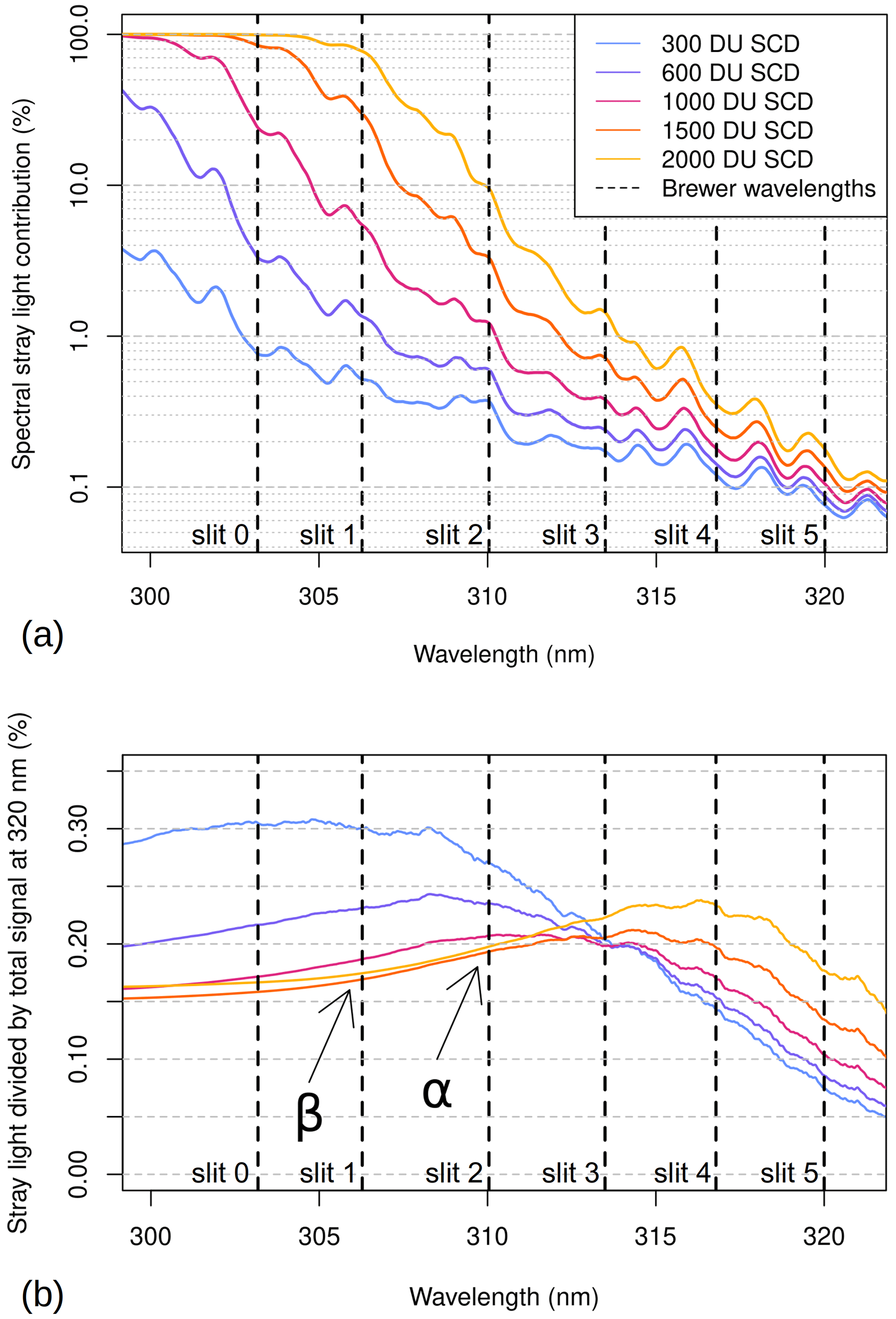
Figure 2 (a) Stray light spectrum simulated for different ozone slant column densities (SCDs), divided by the total signal at each wavelength (“true” solar light, plus stray light). Notice that the vertical scale is logarithmic. The high-resolution spectrum used in the calculations is here downscaled to the Brewer resolution (slit 1) for ease of visualization. (b) Same as above, but the stray light spectrum is normalized to the total signal measured at 320 nm. The vertical dashed lines in both panels indicate the centre wavelengths at which the direct solar irradiance is measured. The experimental characterization of Brewer #009 was used in the calculations.

The same spectra are represented in Fig. 2b after normalization to the total signal at slit 5, I(320 nm). These values are equivalent to the correction factors α and β introduced in Sect. 2.2 for ozone and sulfur dioxide, respectively; i.e., they represent the fraction of light at 320 nm that should be subtracted from the measurements to obtain the “true” count rates. It can be noticed that this factor changes with wavelength and ozone SCD. However, for slits 1 and 2 (306 and 310 nm) and for large ozone SCDs, where it is most relevant, it remains quite stable, with a value of $\mathit{\alpha }=\mathrm{2}\times {\mathrm{10}}^{-\mathrm{3}}$ (or 0.20 %) at slit 2 and slightly lower at slit 1, $\mathit{\beta }=\mathrm{1.7}\times {\mathrm{10}}^{-\mathrm{3}}$ (or 0.17 %). These values refer specifically to Brewer #009 (laser scan, wavelength settings) at a specific time of its life (e.g., when the laser scan was performed). However, by examining results from simulations for several Brewers, it was found, as a general rule, that β is almost always lower than α and that the changes in these coefficients at large ozone SCDs are small. Variations in the ratio plotted in Fig. 2b at slits 1 and 2 for low ozone SCDs should not be a concern, as the stray light effect is negligible in these conditions (Fig. 2a). Likewise, changes in the ratio at longer wavelengths are irrelevant, as the stray light is not an issue for slits 3–5, based on previous discussion and Fig. 2a.

The most important result from the simulations is the finding that the stray light contribution, in count rate space, is relatively constant across the measured wavelengths, making it possible to correct for it in a simple way. This is because the largest contribution to the stray light is due to the brighter irradiance from longer wavelengths that are less affected by ozone. These preliminary calculations give confidence that the method described in Sect. 2.2 has a solid basis, which is confirmed by the simulations shown in Fig. 3. The figure presents the outcome of the Brewer ozone retrieval performed on synthetic solar spectra. If no stray light is included in the spectra (case S1), then the ozone retrieved with the standard algorithm is very close to the true value given as input to the calculations and well within 1 % (the often-cited goal in the Brewer community is to have the Brewers agree to better than 1 %, which is to say the desired precision in the Brewer network is 1 %). Retrievals from measurements affected by stray light (case S2), however, deviate markedly from the true value, and for Brewer #009 they are off by about 1 % at ozone SCDs of 1000 DU (>5 % at 2000 DU). Depending on the geographic location of the Brewer and the average ozone VCD, an SCD of 1000 DU could be reached for an air mass factor lower or higher than 3. Moreover, the ETC is underestimated: the ozone ETC is 2583 for simulation S1 (no stray light) and 2572 for simulation S2 (affected by stray light). This is due to the fact that the Brewer with stray light (S2) was calibrated by transfer from a virtual reference instrument (S1), and the procedure tries to compensate for, on average, the ozone underestimation in the field instrument due to stray light by decreasing the value of the ETC. Quite importantly, the ETC underestimation depends on the chosen (or available) interval of air masses during the calibration procedure. This topic will be addressed in the Discussion (Sect. 4).

When a stray light correction with the proper α coefficient is applied (simulation S3), however, the results are significantly improved and the retrievals are brought back to about the true value even for ozone SCDs of 2000 DU. The improvement is notable, considering that the correction is based on a single free parameter. The value of the ozone ETC in simulation S3, i.e., 2583, matches the one obtained without stray light in the model.

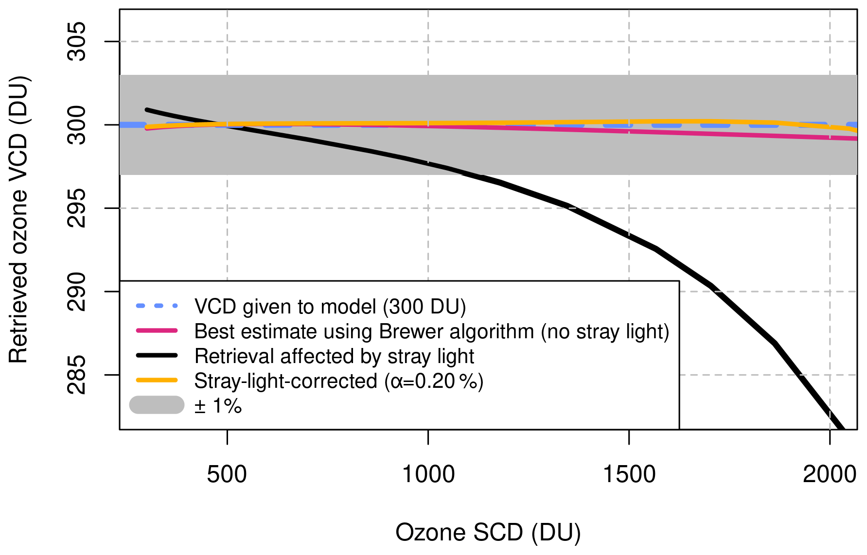
Figure 3 Ozone retrieval technique applied to synthetic solar spectra, as a function of the ozone SCD. The true value provided to the model for this case is 300 DU (dashed blue line). The retrieval with a Brewer unaffected by stray light is plotted as a violet line. The stray light effect is simulated for a single-monochromator Brewer (black line, using the characterization from Brewer #009). Once the correction algorithm is applied to the stray-light-affected spectra, the ozone retrievals overlap again to the true value. The grey band represents the ±1 % interval around the true value.

An important remark is that the α parameter only depends on the instrument, not on the environmental conditions. Indeed, PHYCS was tested with different values for the ozone VCD (250 to 500 DU, reproducing tropical to polar atmospheres), atmospheric pressure, aerosol amount and Ångström exponent, and the value of α providing the best correction was still the same (not shown, as experimental evidence of this property will be given in the next sections).

The same procedure was applied to sulfur dioxide retrievals. In the first case (Fig. 4a), no SO₂ was included in the calculations. This scenario represents a typical situation for most Brewer stations, located far from strong sources of sulfur dioxide. The results show that, in pristine conditions, stray light leads to negative concentrations of SO₂, as frequently observed in the experimental data (Hrabčák, 2018). As in the case for ozone, a proper choice of the β coefficient allows the SO₂ Brewer retrievals to be effectively corrected. In the second case (Fig. 4b), a very high sulfur dioxide VCD (10 DU) was set, likely representative of measurements close to a volcanic plume (e.g., Zerefos et al., 2017). The figure highlights that the same β factor previously determined for pristine conditions still stands in a scenario with high SO₂ concentrations and that PHYCS allows accurate sulfur dioxide retrievals up to rather large air masses (or ozone SCDs). As for ozone simulations, ETC${}_{{\mathrm{SO}}_{\mathrm{2}}}$ is underestimated when stray light is included in the calculations (2243, case S2), while the values are about the same in cases S1 (2279, no stray light) and S3 (2278, corrected with PHYCS). However, as explained in Sect. 3.1, this has little practical implication, since sulfur dioxide only weakly depends on the extra-terrestrial coefficient.

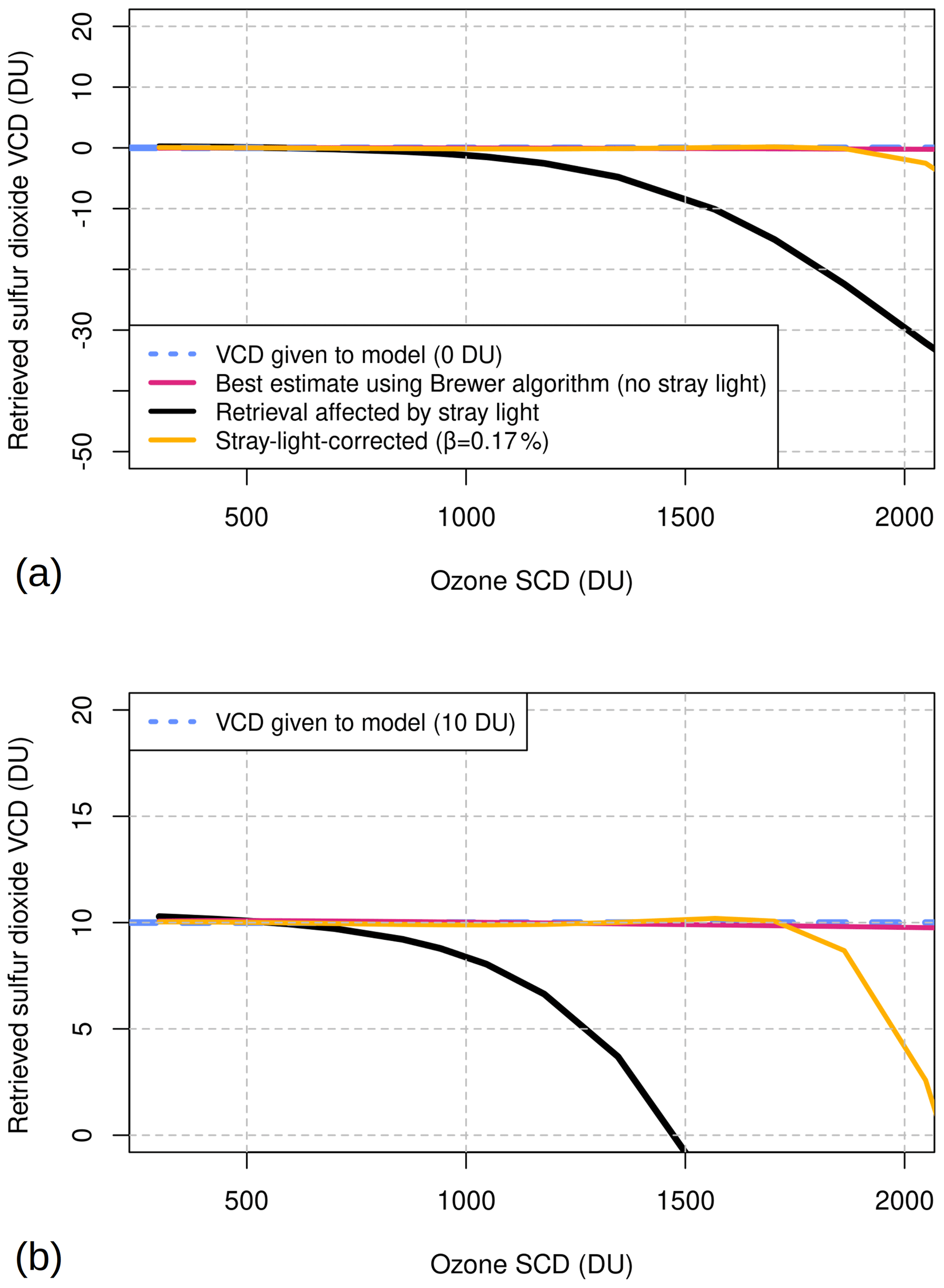
Figure 4 Sulfur dioxide retrievals from the synthetic solar spectra, as a function of the ozone SCD. The true value used in the calculations is (a) 0 DU (dashed blue line) and (b) 10 DU. Notice that the vertical scales in the two panels are different.

Using the calculations, additional hypotheses can be tested. First of all, it can be shown that the algorithm only works if the parameter α, i.e.,  the percentage of the count rates deemed to be representative of the stray light, is calculated with reference to the total signal through slit 5. If α is calculated, e.g., with reference to slit 3 (Fig. S2), then the performances deteriorate significantly. This is due to the fact that wavelengths shorter than 320 nm are strongly affected by ozone absorption; thus they are not a suitable reference to calculate the stray light contribution at slit 2.

A second numerical experiment can be performed to assess the effect of the uncertainty in the stray light correction factors. To this end, the changes observed in the ozone retrievals when using slightly larger (α₊ = 0.3 %) or slightly lower (${\mathit{\alpha }}_{-}=\mathrm{0.1}$ %) correction factors than the optimal one (α=0.2 %, for Brewer #009) were calculated. As evident from Fig. S3a for ozone, variations in α affect the retrievals at large ozone SCDs. It is interesting to note that, conversely, errors in the ETC determination (±10 units in the example, a slightly larger range than expected in ideal conditions) mostly affect the ozone retrievals at small air masses (Fig. S3b). Since α and ETC are uncorrelated, the two unknowns can be determined independently without significant cross talks. Figure S3b also shows that the Bouguer–Lambert–Beer law for the Brewer has a reversed sign (see Appendix A2) and that increases to ETC lead to apparent decreases in ozone.

The same exercise was repeated for sulfur dioxide retrievals by changing either α or β. Figure S4a reveals that the α parameter has an influence on the SO₂ retrievals, as the optical depth of ozone must be subtracted from the total optical depth at 306 nm from which sulfur dioxide is calculated. Therefore, SO₂ calculations are very sensitive to the accuracy of ozone (about −0.5 DU change in SO₂ for every +1 DU change in ozone), which explains why it is necessary to first obtain the correct estimate of α and then for β. Figure S4b instead shows the effect of small variations in β on sulfur dioxide retrievals. The sensitivity to this parameter is also high, and for Brewer #009 variations in sulfur dioxide VCD of ±5 DU at 1800 DU ozone SCD can originate from changes of $\pm \mathrm{2}\times {\mathrm{10}}^{-\mathrm{4}}$ in β. Finally, Fig. S4c highlights that the dependence of the retrieved sulfur dioxide VCDs on ETC${}_{{\mathrm{SO}}_{\mathrm{2}}}$ is very low (about 0.34 DU change in SO₂ for every 10 units in ETC at air mass factor 1).

Finally, a third test was conducted to explore the feasibility of determining the stray light correction coefficients from a Langley plot (Sect. 2.3.2), i.e., without the need of any reference instrument for the transfer of α and β. Figure S5 shows a simulated Langley plot for ozone (R₆ linear combination) with the single-monochromator Brewer #009. Some features are obvious: first of all, the results show that Langley plots with measurements affected by stray light lead to errors in the determination of the ETC, as the linearity of the relation between R₆ and air mass is strongly degraded; second, the method allows an effective correction to the Langley plot, and this fact could be employed to retrieve the correction factors by choosing the α and β values leading to the straightest line, provided that ozone is very stable. It should be noted, however, that the feasibility of this method depends not only on the available air mass range but also on the ozone VCD, as the stray light effect manifests itself at large SCDs (in Fig. S5, the ozone VCD used for the calculations is 300 DU). As mentioned in Sect. 2.3.2, the best sites for Langley plots, i.e., where the ozone VCD is assumed to be the most stable, are located in regions of the world where the ozone layer is thinner; hence the stray light effect might be less evident there due to the lower SCDs. Finally, the figure also shows that the residuals after the stray light correction are even lower than the residuals without stray light in the model. This likely means that the stray light correction also compensates, in small part, for inaccuracies related to the retrieval algorithm itself rather than to the stray light effect. A slight tendency to underestimate ozone at large SCDs by the Brewer algorithm was also found in previous studies (Kiedron et al., 2008). The calculation of instrument-specific weightings in R₆ could help in removing this small residual effect (Savastiouk and McElroy, 2005).

3.2 Application to experimental data

3.2.1 Ozone and sulfur dioxide observations at three Brewer stations

Figure 5 depicts a comparison of the ozone and sulfur dioxide retrievals before and after PHYCS implementation on real data. As described in Sect. 2.1, three locations characterized by very different atmospheric conditions were chosen to test PHYCS in several scenarios.

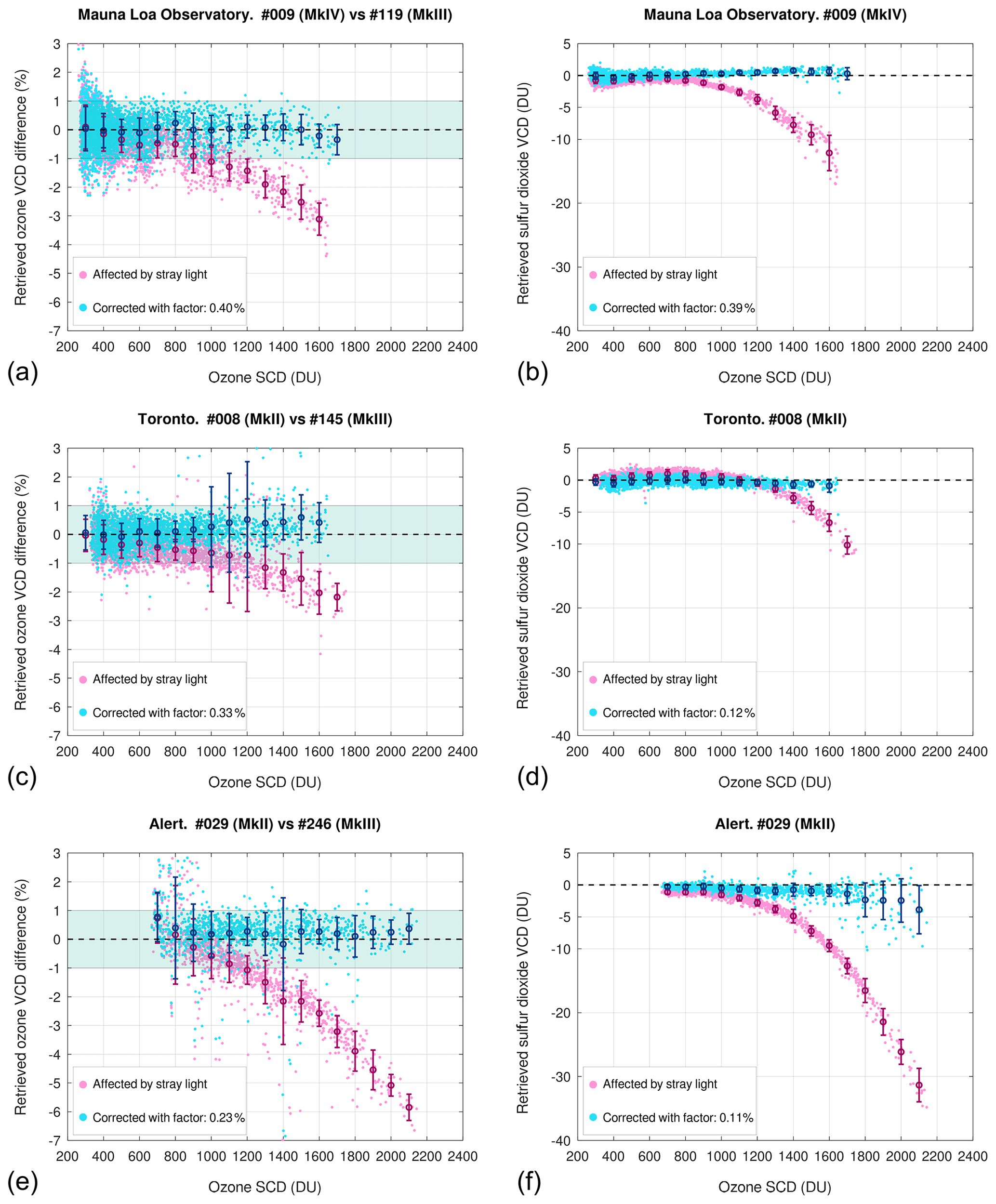
Figure 5 Comparison among retrievals affected by stray light and corrected using PHYCS. (a, c, e) Comparison of ozone VCDs retrieved by three single Brewers at different locations and three co-located double Brewers. The data shown were collected in the period December 2019 to 22 June 2020. (b, d, f) Absolute values of sulfur dioxide VCD retrieved by the three single Brewers before and after stray light reversal. Points represent single measurements pairs (ozone) or individual measurements (sulfur dioxide). The circles and the error bars indicate the average and the standard deviation of data binned at 100 DU ozone SCD intervals.

To assess the performances of the stray light correction on ozone (Fig. 5a, c and e), the retrievals from three single Brewers are compared with the retrievals from co-located MkIII Brewers used as references. Measurement pairs within 5 min from single and double Brewers were considered. Uncorrected data show systematic underestimations of about −2 % to −3 % at 1600 DU ozone SCD at all sites due to stray light. Owing to higher ozone SCDs reached during the year at the Alert site, compared to the other locations, the deviations of the MkII retrievals from the MkIII are as big as −6 % at 2100 DU ozone SCD. However, the new algorithm works well under all atmospheric conditions, and, after application of PHYCS, the corrected values are virtually the same as those retrieved from the double-monochromator spectrophotometers. Indeed, most of the corrected retrievals fall within ±1 % with respect to the double Brewers, even at very large ozone SCDs. At Mauna Loa Observatory, the agreement is better than 1 % up to an ozone SCD of 1900 DU, which corresponds to approximately an air mass factor of 5.5. Field-of-view stray light and very dim light contribute to a high noise level at large solar zenith angles. Points collected at very low SCDs show high retrieval noise, both in the corrected and uncorrected data, owing to minimal absorption by ozone.

The stray light correction factors employed in PHYCS were 0.40 % (MkIV Brewer #009), 0.33 % (MkII Brewer #008) and 0.29 % (MkII Brewer #029), which agree with the stronger stray light effect expected in MkIV Brewers compared to MkII Brewers. Table 3 also reports the factors for the two travelling standards (#017 and #109), with comparable values. It might be noted that the experimental correction factor for Brewer #009 is of the same order of magnitude as the one determined with the model in Sect. 3.1 but larger. This can be due to the simplified assumptions in the calculations, slight discrepancies in the configuration used for the retrieval, and above all the aging of the instrument between the time the laser scan was performed (around the year 2000) and the time when the data shown in the figure were collected (2019–2020). Indeed, stray light has likely increased in the course of 20 years, as shown in Sect. 3.2.5 for Brewer #017. The laser scan that was used for Brewer #009 shows the “wings” at a level of 10⁻⁴. As a test, an offset of 10⁻⁴ was added to the laser scan. With that small addition in absolute sense, the model predicts parameter α to be 0.4 %, the same as in the experimental data. Regarding the ETCs, Table 3 shows that the true extra-terrestrial coefficients are always significantly larger than those originally used to provide (stray-light-affected) retrievals matching the reference measurements. The magnitude of these differences depends largely on the minimum SCD used for the original calibrations, also reported in the table.

Table 3 Configuration of the Brewers used in the study before and after implementing PHYCS. The rows report, in order, the serial number of the reference MkIII Brewer, the α and β coefficients used in the correction, the ozone extra-terrestrial coefficient after the application of the stray light correction, the original extra-terrestrial coefficient used in the Brewer, the difference (ΔETC) between the two values above, and the minimum air mass factor available in the analysis.

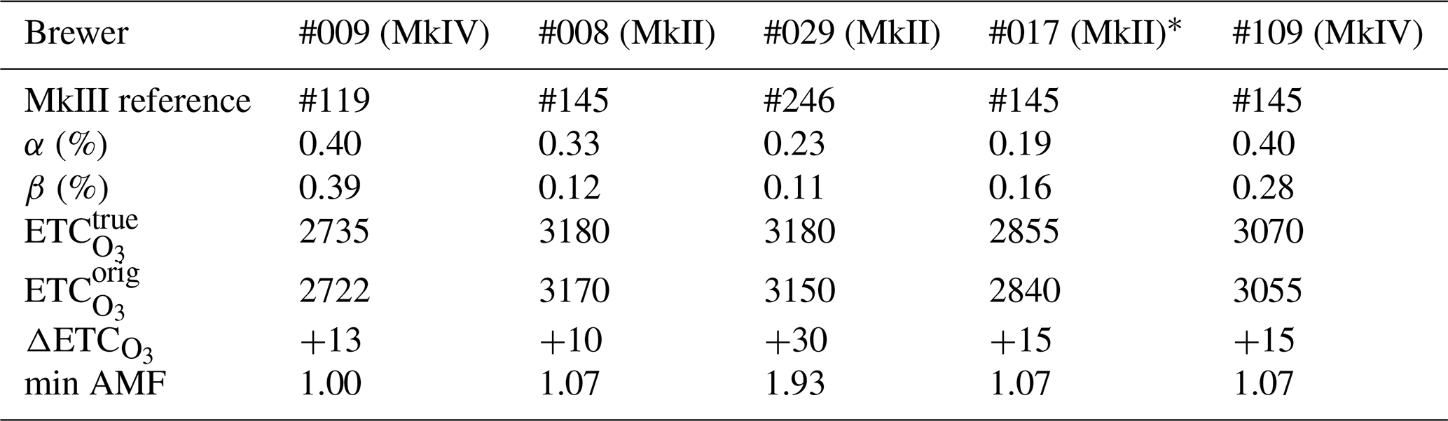
^* Data presented in this table for Brewer #017 correspond to the last row in Table 4.

The results for sulfur dioxide VCDs (Fig. 5b, d and f) similarly show that all corrected data fall within ±1 DU when it is expected to be zero (no strong SO₂ sources close to the stations) and that, after applying PHYCS, the deviation from zero has a similar distribution in both the single and the double monochromator. As predicted by the calculations, the coefficients β used for SO₂ retrievals for the three Brewers are lower than the α's and they comply with the ordering expected by Brewer type (MkIV vs. MkII). The extra-terrestrial coefficients for SO₂ are not reported in Table 3, as sulfur dioxide retrievals show very little sensitivity to variations in ETC, and no change in ETC after applying PHYCS was deemed necessary.

Depending on the atmospheric conditions, sulfur dioxide retrievals can be more or less noisy at extreme ozone SCDs, as seen in these figures. This is because of the very rapid dimming of the shortest wavelength (306 nm) that is only used for SO₂ retrievals. Filtering data with a minimum required count rate at this wavelength can reduce the number of questionable points in the final product. All points where the detected count rate is lower than the estimated stray light contribution should be eliminated.

3.2.2 Sensitivity to stray light coefficients using observations

As done in Sect. 3.1 using simulations, tests were performed on the experimental observations to assess the sensitivity of the stray light correction to α and β. Data from Brewer #009 were employed for that purpose. The α factor was changed to 0.50 % and 0.30 % (its optimal experimental value being 0.4 %), and the maximum changes were of the order of about 1 % for ozone (at 1700 DU ozone SCD) and 1–2 DU for SO₂ (Fig. 6). The same variation in SO₂ was found for much smaller changes in β, its optimum value of 0.39 % for Brewer #009 being changed to 0.41 % and 0.37 %. The results of this test with real observations are similar in magnitude to those from the model, although the experimental data in Mauna Loa do not reach the same large amounts of ozone SCD as in the simulations. A slightly lower sensitivity can be noticed in the real data, which is compatible with the larger correction factors needed in the observations with respect to the calculations.

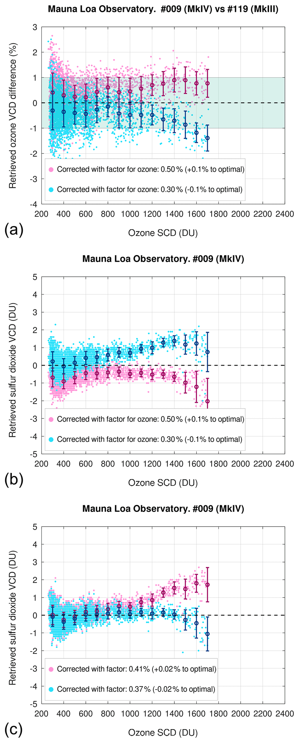
Figure 6 Sensitivity test on real observations from Brewer #009 to assess the variation in (a) the ozone retrievals to small changes in α (an offset of $\pm \mathrm{1}\times {\mathrm{10}}^{-\mathrm{3}}$ to about the optimal value of 0.40 %), (b) the sulfur dioxide retrievals to small changes in α (this latter was again offset by $\pm \mathrm{1}\times {\mathrm{10}}^{-\mathrm{3}}$) and (c) the sulfur dioxide retrievals to small changes in β (offset of $\pm \mathrm{2}\times {\mathrm{10}}^{-\mathrm{4}}$ to about the optimal value of 0.39 %). Notice the different y scales.

If it is assumed that absolute variations of α of $\pm \mathrm{1}\times {\mathrm{10}}^{-\mathrm{3}}$ occur on average in about 10 years (Sect. 3.2.5), we can conclude that in the same lapse of time the ozone retrievals corrected for stray light will still be within 1 % with respect to a MkIII Brewer up to approximately 1700 DU SCD. This same variation in the ozone correction factor affects SO₂ calculations only slightly. A similar period of time is needed to see variations of 1–2 DU in sulfur dioxide due to drifts in β.

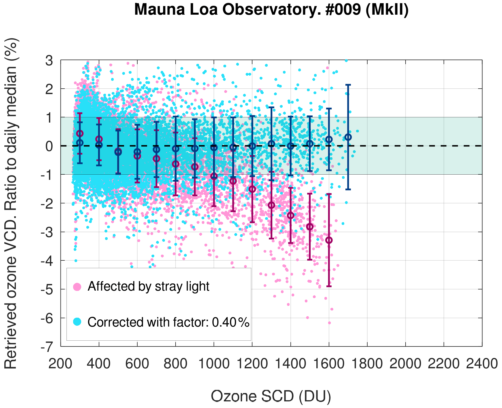
3.2.3 Testing the statistical method

Figure 7 shows an application of the statistical method described in Sect. 2.3.3 with observational data from Brewer #009. For each ozone retrieval, the percentage deviation from the respective daily median VCD is plotted, and then data were binned. Bins with only a few points (<10) were not plotted due to insufficient statistics. The figure shows similar patterns as the comparison with the co-located MkIII (Fig. 5a), with only a slight increase in statistical noise owing to the replacement of actual measurements with daily medians. The results demonstrate that the method is a useful tool for monitoring the validity of the stray light correction factors for those single Brewers that cannot be regularly compared to a double Brewer.

Figure 7 Demonstration of the statistical method for checking the stability of the stray light coefficients (Sect. 2.3.3). The vertical axis represents the percentage deviation of individual ozone retrievals from their respective daily median VCD. Data are binned every 100 DU SCD.

3.2.4 Effect of different atmospheric conditions

To study the effect of different atmospheric conditions, all data from the nine locations visited by Brewer #109 in 2022 were merged together, and PHYCS was applied using fixed coefficients to the whole data set. Then, the statistical method described in Sect. 2.3.3 was used to check the performances of the stray light correction. Despite some noise, it is clear from Fig. 8 that PHYCS worked well at all sites and that the α coefficient did not vary markedly with the location. The same is true for sulfur dioxide: the absolute values of the corrected SO₂ retrievals, always close to zero, show that a unique β coefficient provided an accurate correction for stray light at all sites. The results show that α and β mainly depend on the characteristics of the instrument.

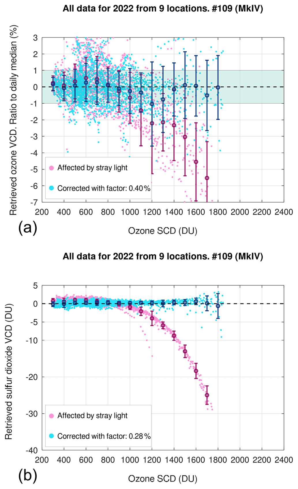
Figure 8 Test to assess the effect of location on the stray light correction. All data from nine locations visited by Brewer #109 in 2022 were merged together. (a) Results from the statistical method. (b) Retrieved sulfur dioxide VCD.

3.2.5 Changes in stray light with time

Data from MkII Brewer #017, together with data from various MkIII Brewers over a number of years, were used to establish historical values for the stray light correction factors. The series were examined in search of retrievals of ozone and sulfur dioxide from the two types of instruments. For this to be done, a large enough range of ozone SCDs is needed, which was not always available in the early years due to the measurement schedules. Late spring was considered the best period for measurements in Toronto, as ozone VCDs are still large and the range of air mass factors is rather wide. A first comparison with data collected in 1993, when MkIII Brewers became operational, was made. Other comparisons at regular intervals were performed so that increases of about 0.1 % in α could be tracked. Table 4 presents the results for some of the comparisons. It is clear that the stray light increased over the life of the instrument, α changing from 0.20 % to 0.40 % and β from 0.17 % to 0.22 %. In 2019, the spherical mirror in the monochromator of Brewer #017 was replaced with a brand new one. The instrumental modification evidently had a significant impact on the stray light correction factors, bringing them essentially to the level of the first available comparison with a double Brewer. Not shown here, similar improvements in the correction factor values were seen in all three Brewers that had undergone the main mirror replacement.

Table 4 Stray light correction factors for Brewer #017 from 1993 to 2019.

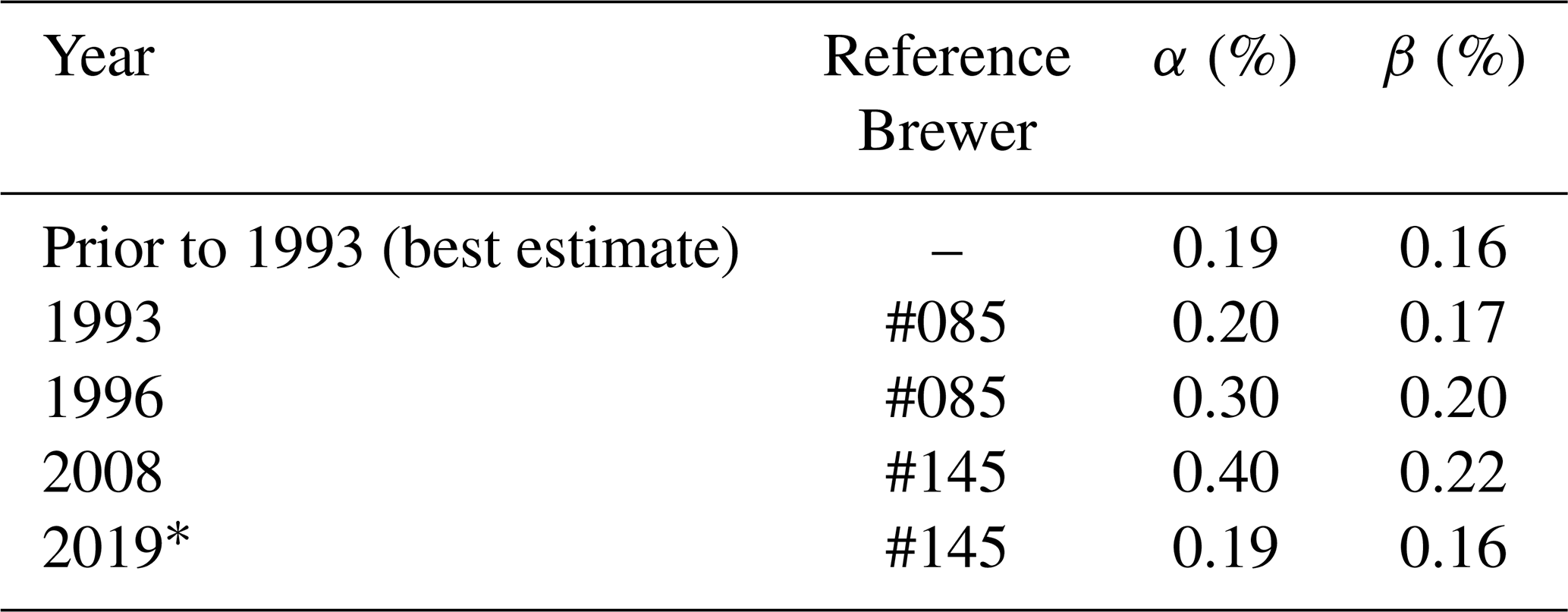
^* A new spherical mirror was installed in Brewer #017 in 2019.

This has three implications in our opinion:

• First, this suggests that the spherical mirror is a major contributor to the internal stray light and the main degrading component in the optics. Dust accumulation is likely to occur there due to both electro- and photophoresis effects while the optics is exposed to bright light.

• Second, it is very likely that the correction factors in the period prior to the first comparison with the double were close to the values in 1993 and 2019 when the spherical mirror was in a similar condition. Thus, our best estimate for the coefficients of Brewer #017 prior to 1993 corresponds to their values in 2019. Even if the former ones were slightly lower, this will not affect the data much and the reprocessing of the entire record of Brewer #017 from 1984 to present using PHYCS is now possible.

• This observation suggests that a visual inspection of the mirror and its replacement or resurfacing would be a useful maintenance consideration on either the basis of inspection or simply an action taken after a considered period of time, especially if the Brewers are expected to continue operating for a long time. It should be noted that resurfacing the mirror would more likely guarantee the instrument would remain in its former alignment (dispersion, slit width).

3.2.6 Uncertainty estimation

Thanks to PHYCS, accurate retrievals from single Brewers are now possible even for large ozone SCDs. Without a proper correction, measurements in such conditions would have normally been filtered out from the analysis by the operator owing to the dominant effect of stray light. The correction for this systematic effect with PHYCS and the resulting extension of the measurement range come at a price, i.e., a slight increase in the overall retrieval uncertainty due to the introduction of the correction itself (BIPM et al., 2010). Here we assess the contribution of the stray light correction to the retrieval uncertainty only for ozone, as sulfur dioxide retrievals are impacted by other and more important sources of uncertainty (Fioletov et al., 2016; Zerefos et al., 2017).

The best way to assess the contribution of the stray light correction to the ozone retrieval uncertainty is to start from Eq. (2), which is the mathematical representation of PHYCS, and to consider how the uncertainty in the different terms propagates to ozone. Three sources of uncertainty can be identified:

• The first source is uncertainty in the counts measured at 320 nm, I(320 nm). This component is dominated by Poisson noise in photon-counting detectors and is expected to increase at very large SCDs. It can also depend on the sensitivity of the particular Brewer and on the dark counts. Kerr (2002) and Gröbner and Meleti (2004) state that the Brewer direct irradiance measurements can reach a precision of 0.1 %, limited by Poisson noise. Additional calculations show that at slit 5 Poisson noise is <1 % even for solar zenith angles slightly larger than 80^∘, where uncertainties from other parameters become more important. Therefore, even if an extreme value of 1 % is considered for random noise in I(320 nm), this would trigger the same effect on the stray light estimate I_s as a change of $\pm (\mathrm{0.01}\times \mathit{\alpha }$) in α due to their relation in Eq. (3). Based on the results presented herein, α is always lower than about 0.65 %, and simulations show that Poisson noise in I(320 nm) would result in uncertainties <0.2 % in ozone (through the stray light correction) at 2000 DU SCD.

• The second source is uncertainty in the correction coefficient α. This component, in turn, is the sum of the following factors:

  • a.

    The first factor is the uncertainty propagated from the reference instrument employed for the calibration transfer to the field instrument, in case the former has already been calibrated and corrected for stray light. If the reference did not need any correction, this term is not considered.

  • b.

    The second factor includes the accuracy and repeatability of the α estimate, depending on the available experimental data and on the method used by the operator to find the correction coefficient leading to the best match with the reference. Some tests were made by limiting the available data to <1000 DU SCD, and the effect when the α factor changed by $\pm \mathrm{1}\times {\mathrm{10}}^{-\mathrm{4}}$, however small, was still visible. Hence, the stray light correction coefficient can be determined to within $\pm \mathrm{1}\times {\mathrm{10}}^{-\mathrm{4}}$. Based on radiative transfer calculations, this translates into the retrieved ozone as a change in ±0.2 % at 1800 DU SCD and ±0.3 % at 2000 DU SCD.

  • c.

    The third factor includes drifts in α with time (Sect. 3.2.5), which include both an increase in stray light due to aging of the instrument and variations in the spectral sensitivity of the Brewer, altering the solar spectrum “seen” by the instrument. For a well-maintained Brewer, we assume that α does not drift by more than $\pm \mathrm{1}\times {\mathrm{10}}^{-\mathrm{4}}$ before the next calibration, hence the same results as in case 2b can be used.

• The third source is the uncertainty in the mathematical model itself, which depends on the reliability of the underlying assumptions. The deviations from these assumptions can vary among instruments, e.g., based on the laser response shown in Fig. 1, therefore this factor is considered to be uncorrelated among Brewers. A rough estimate of the model uncertainty can be obtained from Figs. 5a, c and e, and examining the deviations of the bin averages from the 0 % reference line. As the residuals are always within ±0.5 %, the resulting uncertainty provided by this factor is about $\mathrm{0.5}\mathit{\%}/\sqrt{\mathrm{3}}=\mathrm{0.3}\mathit{\%}$ if it is assumed that errors from the simplified model are uniformly distributed.

Each successive level in the transfer of the stray light calibration leads to slightly larger uncertainties in that the uncertainty in the reference instrument data is propagated to the secondary instrument. Assuming that the number of simultaneous measurements collected during the transfer is large, we can neglect Poisson noise from the primary instrument in the uncertainty in the secondary instrument. Table 5 summarizes the factors considered here and the total contribution of the stray light correction to the uncertainty in individual ozone retrievals. In the extreme case of 2000 DU ozone SCD, this contribution is 0.6 % for primary instruments (e.g., calibrated from an instrument without stray light) and 0.8 % for secondary instruments (i.e., calibrated with an instrument already characterized for the stray light effect). These are most likely very conservative (worst case scenario) estimates.

Table 5 Maximum (at 2000 DU ozone SCD) contribution of the stray light correction to the uncertainty in ozone retrievals for primary and secondary instruments.

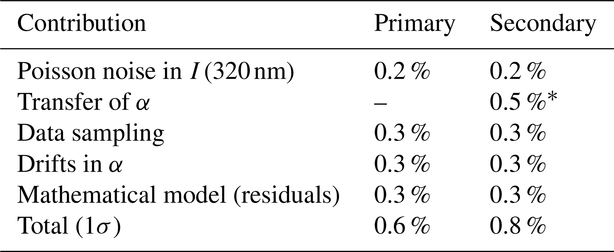
^* Poisson noise in the primary instrument is not propagated to the secondary instrument since the number of simultaneous measurements is assumed to be large.

3.2.7 MkIII Brewers and stray light

The available laser scans (Fig. 1) show that the expected level of stray light in double-monochromator Brewers is very low, but it is not zero. To our knowledge, no study of stray light in MkIII Brewers exists. The spectral sensitivity curve in double monochromators is usually a monotonically and rather steeply increasing function of wavelength. This can magnify the potential effect of stray light, since the shortest wavelengths are relatively dimmer than those in the single-monochromator instruments given the same light level at the longest wavelength. In addition, the absence of any cut-off filters in the MkIII Brewers can increase the available long-wavelength radiation scattered inside the instrument to reach the detector.

One way to assess whether MkIII Brewers have effects from stray light is to look at the sulfur dioxide retrievals at large ozone SCDs. In some cases, where observations are done at ozone SCDs larger than 1600 DU, the sulfur dioxide retrieved values show significant underestimations with respect to the expected value of 0 DU (Fig. S6). Applying our algorithm to the data with no correction for ozone and only a very small correction factor for SO₂ completely compensates for the effect, and the value of 0 DU is retrieved over the whole ozone SCD range as expected. The correction factor β needed for MkIII is an order of magnitude lower than that for single-monochromator instruments. While this simple test is not conclusive, it may suggest that a further investigation of stray light in MkIII Brewers might be useful.

4 Discussion

The discussion now focuses on the following question: why should a Brewer user implement the stray light correction described in this study? Here follows a list of some reasons:

1. First of all, PHYCS allows access to a larger range of ozone SCDs and air mass by the Brewer. The common practice of cutting the measurements at large solar zenith angles potentially introduces some biases and might not solve the stray light issue for the most affected Brewers. Also, measurements at different air masses, both small and large, may be of interest, for example, to studies on ozone trends in different layers of the atmosphere (Fountoulakis et al., 2021).

2. Partially connected to the previous point, a further issue triggered by the presence of stray light, as illustrated in Sect. 3.1 and 3.2.1, is the underestimation of the extra-terrestrial coefficient resulting in a calibration transfer. To further complicate things, the magnitude of this underestimation depends on the range of air masses available during a specific calibration campaign. Generally speaking, an erroneous ETC is not a real problem as long as measurements are always performed at ozone SCDs comparable to those when the ETC was determined. Indeed, the aim of a calibration transfer is to make ozone retrievals from the field instrument agree with the reference. However, air mass changes throughout the day and the seasons, which can induce biases with cycles on different temporal scales. Additionally, if a Brewer calibrated in such a way is transported to locations at different latitudes and operates with very different ozone SCDs, its calibration might not be suitable for the new site. A not dissimilar case is when Brewers normally operating at high latitudes are calibrated at low latitudes during intercomparison exercises. As during the transfer the ETC is normally calculated to match the ozone VCD from the reference at low air masses, the calibration might not be accurate when the instrument returns to its original location and operates at larger SCDs.

   For example, the data from Brewer #009 at MLO show ozone underestimation approaching 1 % at slant ozone of approximately 800 DU (Fig. 5a). If this instrument were to be moved to Alert, where the minimum measured slant ozone amount is just less than 800 DU (Fig. 5e), then with the current calibration the ozone VCD would be underestimated all year round. In contrast, Brewer #029, having its calibration done on site in Alert, provides the data to within 1 % up to 1200 DU of ozone in the path.

   It should be noted that for specific Brewers strongly affected by stray light, the only way in the past to bring their ozone retrievals close to the reference Brewer during calibration was not only to adjust the ETC, but also to let the ozone absorption coefficient vary (the so-called “two-point calibration”). Therefore, the value of the latter could be different from that calculated analytically based on the laboratory cross-sections. Although the agreement to the reference was all artificial, as both ETC and absorption coefficient were wrong, and still limited to approximately 1000 DU ozone SCD, any other combination would lead to erroneous values of ozone at almost any SCD. This practice should be discontinued in favour of using PHYCS.

3. Having a single parameter in PHYCS for ozone gives a quantitative measure of the stray light effect for each Brewer. This can be used as a tool for assessing the state of the instrument optics.

4. As quantitatively discovered for the first time, the magnitude of the stray light effect can change during the lifetime of a Brewer. When long-term trends are to be studied, this factor should be considered in order not to introduce fictitious trends, which will specifically depend on the ozone SCD. On a relative scale, as also mentioned by Kiedron et al. (2008), the increase in stray light effect with time might have larger relative effect for MkIII Brewers. This directly addresses the issue of whether long-term ozone trends have been miscalculated when single Brewers have been replaced by double Brewers, particularly at high-latitude stations.

5. Past calibrations when either the reference or the field Brewer, or both, instruments were affected by stray light need to be reprocessed using PHYCS and the data from the field Brewers need to be reanalyzed.

6. While the algorithm is easy to implement, the sheer volume of the Brewer data makes this task both important and time-consuming, requiring additional resources to do it right. It should be stressed that not all data centres are able to track and/or identify changes in the submitted data, which will lead to challenges for the data end users when some data have been corrected and some have not.

7. As PHYCS is implemented at a very early stage of the Brewer data reduction, the same method could be easily adapted to other measurement geometries and techniques in addition to the direct-sun method (e.g., zenith sky, Umkehr). Although further advances are needed, PHYCS could contribute to drastically improve the quality of SO₂ retrievals with Brewers.

8. In our tests using the data from over 100 Brewers for the last 10 years, the standard lamp (SL) ratios R₆ and R₅ change slightly when PHYCS is applied to the SL count rates. However, that change is constant over time even when the ratio values were changing significantly. Since the application of the standard lamp correction to the measurement data is based on the differences between the reference and the current SL ratio values, the effect of PHYCS is negligible. As long as PHYCS is either applied or not applied to the SL data consistently, there will be no effect on the retrievals.

In summary, once PHYCS has been implemented, the Brewer network will be able to consistently provide reliable data at large slant ozone columns. At high latitudes, this will translate to more data availability throughout the year. High-quality Brewer calibrations performed on-site, especially at middle and high latitudes, will be easier using a more portable single-monochromator Brewer. Consistency of the data quality collected with the Brewers of different ages (and thus different stray light contributions) will be significantly improved.

The simplicity of the algorithm allows it to be easily implemented in the data processing, either by the principal investigators for individual instruments or by central authorities like the World Ozone and UV Data Centre (WOUDC) and/or the European Brewer Network (EUBREWNET). To this aim, we have developed rmstray, a dedicated multi-platform software package implementing PHYCS, and we have made it available to the Brewer users (Savastiouk and Diémoz, 2023). Also, the most popular Brewer ozone data processing software, O3Brewer (Stanek, 2023), has now been modified to include PHYCS. Past calibrations can be used to re-evaluate the series with no need for additional data. Moreover, the analysis shows that the correction factors for the algorithm change slowly. As an example, for Brewer #017 a change in the ozone factor of 0.1 % and in the sulfur dioxide factor of 0.02 % was found approximately every 10 years. This suggests that a usual calibration frequency for the Brewers of 1–3 years is sufficient to keep the stray light correction factors up to date with no effect on the data.

As a simpler alternative for the Brewers that have no calibration for stray light correction, the operator can use some typical values from this study. Indeed, to establish a range for the correction factors, we analyzed over 20 Brewers, both MkII and MkIV. While the upper limit was actually similar in both types, the minimum values were significantly different. The range of α for the MkII was 0.19–0.6 and for the MkIV it was 0.4–0.65. The lowest ozone correction factors are likely an underestimate, but using them will definitely extend the range of ozone SCDs to make the data consistent with stray-light-free instruments. For the ETC adjustment, the noon values for ozone VCD can be replicated for the data with and without the stray light correction as the best available estimate in these cases.

In conclusion, we have two final remarks. First, in this work ozone absorption coefficients based on the Bass and Paur (1985) cross-sections were used. Since this is a simple scaling factor, it has no effect on the corrections for stray light. This also means that if the Brewer community switches to other cross-sections in the future, the stray light correction parameters will not change. Second, stray light is not expected to affect Brewer retrievals obtained in the visible range, such as nitrogen dioxide from MkIV instruments (Diémoz et al., 2021) or AOD in the interval 425–453 nm (Diémoz et al., 2016), since the spectral gradient of the solar irradiance is less pronounced in this band.

5 Conclusions

A new method, the PHYsically based Correction for Stray light (PHYCS), was developed to correct for stray light in Brewer spectrophotometers, and its implementation as a software package is now available to the user community. PHYCS corrects the count rates collected by the instrument at the very beginning of the standard data reduction; therefore it can be used upstream of any additional software normally employed by the operator and does not require further modifications of the processing chain. Radiative transfer calculations were performed to verify the assumptions at the basis of PHYCS and to provide a first guess of the correction parameters. The effectiveness of the method was then showcased using real-world data from several Brewers. Once applied, PHYCS allows the retrieval of ozone and sulfur dioxide from single-monochromator instruments within ±1 % and ±1 DU, respectively, to those from double-monochromator Brewers even at large ozone slant column densities. Only one free parameter for ozone and one for sulfur dioxide are needed for the method, and they can be easily transferred during calibrations or retrieved by Langley plot analysis. An additional method is proposed to monitor the stability of the stray light effect with time. The uncertainty brought by the stray light correction to the overall ozone uncertainty is estimated to be well below 1 % even for ozone SCDs of 2000 DU.

In addition to the aforementioned findings, this research has yielded further outcomes that contribute to understanding the ozone and sulfur dioxide measurement. For the first time, using a data set longer than 30 years, this analysis has provided evidence that stray light can increase during the lifetime of an instrument, which can propagate in the calculation of the trends as a function of the ozone slant path. On another topic, although more investigations are required, the analysis has raised the possibility that even MkIII Brewers could be marginally affected by stray light, especially at the shortest wavelength used for sulfur dioxide retrievals.

PHYCS is already being tested at single stations, such as the Boundary Layer Air Quality-Analysis Using Network of Instruments (BAQUNIN) supersite promoted by the European Space Agency (Iannarelli et al., 2022), and can be readily implemented by central authorities like the World Ozone and UV Data Centre (WOUDC) or the European Brewer Network (EUBREWNET). In the near future, it is planned to test the algorithm for other observation geometries, different ozone retrievals techniques (e.g., Umkehr) and other products such as the aerosol optical depth (López-Solano et al., 2018). Moreover, PHYCS unveils new potential applications to accurately retrieve sulfur dioxide or the effective temperature of the ozone layer with Brewers. Possible adaptations to spectral UV are also not excluded.

Appendix A: Brewer working principles

A1 The Brewer spectrophotometer

The Brewer system consists of a tracker to turn the instrument towards the light source (generally the sun or the moon) and a spectrophotometer. The latter, in turn, is composed of the foreoptics, one or two monochromators, and a detector. The foreoptics include a zenith prism, whose rotation determines the elevation of the observing line of sight, and a set of filters. The monochromator is a modified Ebert type that uses diffraction gratings to create a spectrum at the exit slit plane. The number of monochromators and the type of gratings determine the type of the Brewer:

• MkII Brewers are single-monochromator instruments with a 1800 lines mm⁻¹ grating delivering the UV spectrum in the second order. MkV are just MkII Brewers with a modified filter wheel to be able to switch from UV to visible.

• MkIV Brewers are single-monochromator instruments with a 1200 lines mm⁻¹ grating producing the UV in the third order (and visible in the second order to retrieve nitrogen dioxide).

• MkIII Brewers have two monochromators and use 3600 lines mm⁻¹ gratings so that the UV spectrum is in the first diffraction order.

The gratings in all Brewer modifications can be turned with a high-precision micrometer screw to select the portion of the spectrum that lands on six fixed exit slits. A single photomultiplier tube (PMT) is used as the detector.

To keep the wavelength setting in the Brewer stable, the diffraction grating is not turned during the direct-sun (DS) observations and the selection of the wavelengths is done instead by a fast-moving shutter that opens one exit slit at a time. Nominally, at the ozone operating position these exit slits are at 302, 306, 310, 313, 317 and 320 nm, with slight variability among the instruments. The convention is to number the exit slits 0 through 5. Slit 0 is mostly employed for wavelength calibration using an internal mercury lamp.

A2 Standard Brewer direct-sun retrieval algorithm for ozone and sulfur dioxide

The standard Brewer DS observation is a set of five individual measurements of solar radiation at the six slits plus a dark count reading. The standard Brewer algorithm first converts the detected counts into count rates by dividing the accumulated counts by the integration time. Next, count rates at each slit j from 0 to 5, $I_{{\mathrm{d}}_j}$ (the subscript d stands for “detected”), are corrected for the dark count rate, stray light contribution (when PHYCS is implemented) and linearity.

These count rates are converted into logarithmic space:

$$\begin{array}{}\text{(A1)}& F_{{\mathrm{d}}_j}={\mathrm{10}}^{\mathrm{4}}{\log }_{\mathrm{10}}{I}_{{\mathrm{d}}_j}.\end{array}$$

For reasons related to the limits in the computer memory at the time of the Brewer invention, the Brewer algorithm uses logarithm base 10 multiplied by 10⁴ and performs most operations after that with integer numbers. Using the Bouguer–Lambert–Beer law (Bouguer, 1729) for radiation extinction in logarithmic form and with the assumption that only aerosol, air, ozone and sulfur dioxide absorb/scatter strongly in the part of the spectrum that is measured by the Brewers, we can write

$$\begin{array}{}\text{(A2)}& \begin{array}{rl}{F}_{{\mathrm{d}}_j}=& F_{{\mathrm{0}}_j}-\left({\mathrm{10}}^{\mathrm{4}}{\log }_{\mathrm{10}}e\right)\\ & [{\mathit{\mu }}_{\mathrm{aerosol}}{\mathit{\tau }}_{\mathrm{aerosol}}+{\mathit{\mu }}_{\mathrm{air}}{\mathit{\tau }}_{\mathrm{air}}+{\mathit{\mu }}_{{\mathrm{O}}_{\mathrm{3}}}{\mathit{\tau }}_{{\mathrm{O}}_{\mathrm{3}}}+{\mathit{\mu }}_{{\mathrm{SO}}_{\mathrm{2}}}{\mathit{\tau }}_{{\mathrm{SO}}_{\mathrm{2}}}],\end{array}\end{array}$$

with $F_{{\mathrm{0}}_j}$ being the logarithm base 10 of the count rates that would be detected outside of the Earth's atmosphere, μ the air mass factor needed to convert the slant column density (SCD) into the vertical column density (VCD) and τ the optical depth for the corresponding compounds. In the Brewer algorithm, $F_{{\mathrm{0}}_j}$ values are explicitly corrected for the air (Rayleigh) scattering τ_air since it is easily calculated. μ is calculated with the current algorithm using the solar zenith angle at the time of the measurement and the effective layer height of each compound.

Linear combinations of $F_{{\mathrm{d}}_j}$, i.e., R₆ and R₅, commonly called the second ratios since they are effectively logarithms of count rate ratios, are computed to make R₆ almost exclusively sensitive to ozone and R₅ almost exclusively sensitive to sulfur dioxide and ozone.

$$\begin{array}{}\text{(A3)}& R_{\mathrm{6}}=-F_{{\mathrm{d}}_{\mathrm{2}}}+\mathrm{0.5}{F}_{{\mathrm{d}}_{\mathrm{3}}}+\mathrm{2.2}{F}_{{\mathrm{d}}_{\mathrm{4}}}-\mathrm{1.7}{F}_{{\mathrm{d}}_{\mathrm{5}}}\end{array}$$

$$\begin{array}{}\text{(A4)}& R_{\mathrm{5}}=-F_{{\mathrm{d}}_{\mathrm{1}}}+\mathrm{4.2}{F}_{{\mathrm{d}}_{\mathrm{4}}}-\mathrm{3.2}{F}_{{\mathrm{d}}_{\mathrm{5}}}\end{array}$$

Note that both $F_{{\mathrm{d}}_{\mathrm{1}}}$ and $F_{{\mathrm{d}}_{\mathrm{2}}}$ are used with the coefficient of −1. These are, as we mentioned earlier, the values mostly affected by the stray light. The effect of the stray light then is an underestimation of R₆ and R₅.

The ozone differential absorption coefficient (in units cm⁻¹) for R₆, referred to as A₁ in the Brewer operating software, and the ratio of the sulfur dioxide absorption coefficient to the ozone absorption coefficient for R₅, referred to as A₂, are calculated as part of the instrument characterization using the dispersion test results and laboratory-provided cross-sections for ozone and sulfur dioxide. Absorption coefficients are calculated as a linear combination of cross-sections that have been convolved with the measured slit functions. Currently, cross-sections are used at a constant effective ozone temperature of −44 ^∘C. Another differential absorption coefficient A₃ is calculated for R₅ using the ozone cross-sections to account for the sensitivity of R₅ to ozone. When computing the linear combination of the cross-sections, the result comes out negative, but out of convenience, A₁, A₂ and A₃ are defined as positive, and, to compensate for that, the sign of the other terms in the Bouguer–Lambert–Beer law is reversed as well. The extra-terrestrial coefficients for R₆ and R₅, i.e., ETC${}_{{\mathrm{O}}_{\mathrm{3}}}$ and ETC${}_{{\mathrm{SO}}_{\mathrm{2}}}$, are determined by a calibration process, as discussed later.

Now, the total ozone column $X_{{\mathrm{O}}_{\mathrm{3}}}$ in Dobson units (DU) can be calculated as

$$\begin{array}{}\text{(A5)}& X_{{\mathrm{O}}_{\mathrm{3}}}={\displaystyle \frac{R_{\mathrm{6}}-{\text{ETC}}_{{\mathrm{O}}_{\mathrm{3}}}}{\mathrm{10}{A}_{\mathrm{1}}\mathit{\mu }}},\end{array}$$

and the sulfur dioxide column $X_{{\mathrm{SO}}_{\mathrm{2}}}$ becomes

$$\begin{array}{}\text{(A6)}& X_{{\mathrm{SO}}_{\mathrm{2}}}={\displaystyle \frac{R_{\mathrm{5}}-{\text{ETC}}_{{\mathrm{SO}}_{\mathrm{2}}}-\mathrm{10}{X}_{{\mathrm{O}}_{\mathrm{3}}}{A}_{\mathrm{3}}\mathit{\mu }}{\mathrm{10}{A}_{\mathrm{2}}{A}_{\mathrm{3}}\mathit{\mu }}}.\end{array}$$

The factor 10 accounts for the fact that the F values were multiplied by 10⁴ and that 1 DU $={\mathrm{10}}^{-\mathrm{3}}$ cm.

A3 Calibration of the Brewer spectrophotometer

The two commonly used methods for determining the ETCs for ozone and sulfur dioxide are the absolute calibration with the Langley plots (Langley, 1903) and a transfer of the calibration from another Brewer that has been already calibrated. Both methods are described in detail elsewhere (e.g., Redondas et al., 2018). Notably, in the calibration transfer method, two instruments take quasi-simultaneous DS measurements, and then the ozone values from the reference (ref) instrument, $X_{{\mathrm{O}}_{\mathrm{3}}}^{\mathrm{ref}}$, are used in Eq. (A5) for the instrument to be calibrated (new):

$$\begin{array}{}\text{(A7)}& X_{{\mathrm{O}}_{\mathrm{3}}}^{\mathrm{ref}}={\displaystyle \frac{R_{\mathrm{6}}^{\mathrm{new}}-{\text{ETC}}_{{\mathrm{O}}_{\mathrm{3}}}^{\mathrm{new}}}{\mathrm{10}{A}_{\mathrm{1}}^{\mathrm{new}}\mathit{\mu }}},\end{array}$$

and ETC${}_{{\mathrm{O}}_{\mathrm{3}}}^{\mathrm{new}}$ is calculated. An average of these from a number of observations is used as the calibrated value. Assuming that the reference Brewer has no measurable stray light and ozone is calculated correctly from its measurements, the calibrated ETC value will be underestimated if the Brewer to be calibrated has measurable stray light. This is important to remember when correcting for the stray light effect. Conversely, in an unlikely event where the reference Brewer has stray light and the new Brewer does not, then the ETC is overestimated.

Appendix B: Details on simulations

B1 Input data

In order to reproduce the Brewer behaviour, experimental data from the ordinary characterization of a specific instrument are needed:

• This includes centre wavelength and resolution relative to each slit. These data, needed to simulate the core region of the instrumental bandpass function, are taken from the dispersion (DSP) test.

• Laser scans at 325 nm (Fig. 1) are used to simulate the amount and the effect of stray light in the shoulder and wing regions. Details are provided in the next section.

• Brewer spectral sensitivity is needed to simulate the solar spectrum actually “seen” by the Brewer. The response through the direct port is here approximated by the UV response measured through the global entrance port (UV diffuser). There are small differences in the optical settings for the two observation geometries: the UV dome diffuser is not used for direct-sun measurements and an internal ground quartz filter is added for direct sun. However, both components are assumed to be very neutral in colour. Everything else is the same in both observation geometries, including the components that introduce most of the spectral sensitivity observed in the Brewer, i.e., the photomultiplier detector, the UV combination filter and to a lesser extent the neutral density filters.

  As highlighted by Kiedron et al. (2008), it should be noted that the UV response is normally measured with a lamp and that the response itself is affected by stray light. However, the same authors show that the effect is negligible in the spectral range of interest.

B2 Spectrum calculation

We calculate the direct component of the solar irradiance reaching the Earth's surface, I(λ), by the Bouguer–Lambert–Beer law accounting for air molecules, ozone, sulfur dioxide and aerosols in the atmosphere. The configuration of the main parameters is reported in Table B1. The calculation of the spectrum extends over the wavelength range 280–400 nm. It is performed at high resolution (0.005 nm) to accurately account for the spectral structures in both the solar spectrum and the ozone cross-section within the Brewer slit bands. We do not simulate solar irradiance at wavelengths longer than 400 nm as we assume that the Brewer responsivity is low in that range due to a combined effect from the PMT sensitivity dropping off and the UV combination filter and that the contribution of out-of-range stray light is negligible (Pulli et al., 2018). Average atmospheric midlatitude conditions are employed for most of the simulations. In the base scenario, we set the sulfur dioxide VCD and AOD to zero; however, these values were changed for specific tests. It should be noted that the model configuration, including the extra-terrestrial spectrum and the choice of the ozone and sulfur dioxide cross-sections, has a very limited impact on the simulated stray light effect, which mostly depends on the Brewer characterization (laser line) and the ozone slant column.

Coddington et al. (2021)Bodhaine et al. (1999)Bass and Paur (1985)Redondas et al. (2014)Gorshelev et al. (2014)Serdyuchenko et al. (2014)McGee and Burris (1987)Ångström (1929)

Table B1 Main parameters employed in this work to simulate the solar spectra.

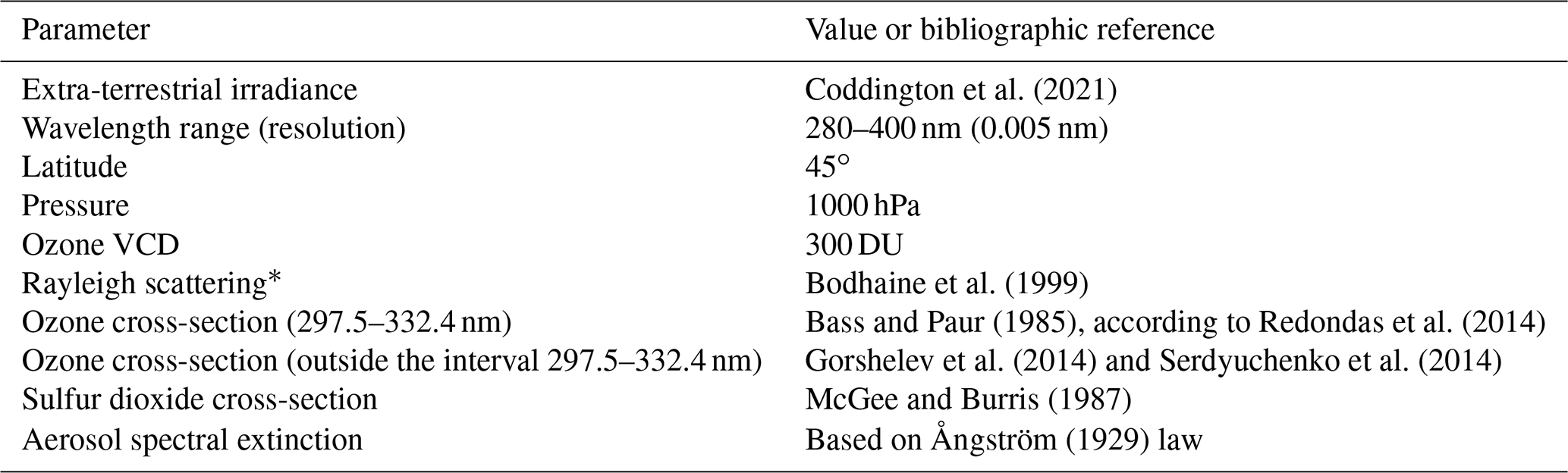
^* Only used to simulate the solar spectrum and the stray light spectrum but not included when retrieving species; see details in Appendix B2.

We treat the effect of the stray light and the finite resolution of the instrument separately:

• 1.

  To simulate the stray light effect, we assume that measurements of the laser emission line at 325 nm outside the in-band interval are representative of the Brewer stray light response to any input wavelength. Therefore, similarly to Zong et al. (2006), the scans are normalized to the integral within the in-band region f_IB(λ) and this “core” region is set to zero, as we simulate the effect of the finite resolution in a different way. The resulting function, f_SL(λ), is then convoluted with the solar spectrum to provide an estimate of the stray light spectrum S(λ), i.e.,

  $$\begin{array}{}\text{(B1)}& S\left(\mathit{\lambda }\right)=\int I\left({\mathit{\lambda }}^{\prime }\right)R\left({\mathit{\lambda }}^{\prime }\right)f_{\mathrm{SL}}(\mathit{\lambda }-{\mathit{\lambda }}^{\prime })d{\mathit{\lambda }}^{\prime }.\end{array}$$

  R is the Brewer responsivity. The sign of the argument in f_SL is due to the fact that the laser spectrum was obtained as a scan; i.e., the count rates recorded at wavelengths shorter than the laser peak are due to the stray light from longer wavelengths. The missing “right wing” of the scans in single Brewers (owing to the reduced spectral range of these instruments, only up to 328 nm) is unimportant, as solar radiation from shorter wavelengths does not significantly affect the count rates measured at longer wavelengths.

  It should be highlighted that obtaining the stray light spectrum as a convolution in the wavelength space is only an approximation of the real stray light (some comments are given in Sect. S1 of the Supplement). Thus, such results should not be used to correct the Brewer data. Anyway, they provide a convenient framework to study the stray light behaviour with sufficient accuracy for our purposes.

  Stray light can be switched off/on in the model depending on the considered case, i.e., S1 or S2–3 (Sect. 2.4). When we want to include the stray light effect, the term in Eq. (B1) is added to the direct irradiance spectrum weighted by the Brewer spectral response (I(λ) R(λ)); otherwise only the latter product is considered.

• 2.

  To simulate the finite resolution of the Brewer at the various slits, the high-resolution spectrum obtained from the previous step is further integrated over each slit function. These latter are approximated as trapezoids, i.e., isosceles triangles cut at 87 % of their height, according to Wardle (2001) (also Moeini et al., 2019), as normally done when processing the results of the dispersion test.

• 3.

  To correct for stray light in the synthetic spectra (S3), a fraction of the simulated count rates at the longest wavelength (slit 5) is subtracted from the count rates of the other slits (notice that this operation must be performed before calculating the logarithm base 10).

B3 Synthetic retrievals

After simulating the solar irradiance measured by the Brewer, the logarithms of the (corrected or uncorrected) count rates are linearly combined as in the traditional Brewer algorithm (Appendix A2), using the standard weighting coefficients.

The effect of molecular scattering along the atmospheric optical path is here compensated for by correcting the linear combination using the same Rayleigh cross-sections employed to calculate I(λ) in place of using the standard Brewer Rayleigh correction. This avoids systematic errors due to the incomplete removal of the Rayleigh scattering in Brewers (Carlund et al., 2017) to focus on the stray light effect only. The ETCs of the virtual Brewer must be determined in order to retrieve O₃ and SO₂. In simulation S1 (Sect. 2.4), they are obtained by iterating the simulations at several air masses and using the Langley extrapolation method, similarly to what is usually done with real-world reference instruments, assuming they have no stray light. In simulations S2–S3, the ETCs are obtained by transfer based on the a priori VCDs given to the model. The absorption coefficients A₁, A₂ (this one set to a fixed value of 2.35, in the standard Brewer algorithm) and A₃ are recalculated for each simulated instrument based on the cross-sections listed in Table B1 and the experimental characterization (measurement wavelengths and resolutions).