Single field-of-view sounder atmospheric product retrieval algorithm: establishing radiometric consistency for hyper-spectral sounder retrievals

The single field-of-view (SFOV) sounder atmospheric product (SiFSAP) retrieval algorithm has been developed to address the need to retrieve high-spatial-resolution atmospheric data products from hyper-spectral sounders and ensure the radiometric consistency between the retrieved properties and measured spectral radiances. It is based on an integrated optimal-estimation inversion scheme that processes data from the satellite-based synergistic microwave (MW) and infrared (IR) spectral measurements from advanced sounders. The retrieval system utilizes the principal component radiative transfer model (PCRTM), which performs radiative transfer calculations monochromatically and includes accurate cloud-scattering simulations. SiFSAP includes temperature, water vapor, surface skin temperature and emissivity, cloud height and microphysical properties, and concentrations of essential trace gases for each SFOV at a native instrument spatial resolution. Error estimations are provided based on a rigorous analysis for uncertainty propagation from the top-of-atmosphere (TOA) spectral radiances to the retrieved geophysical properties. As a comparison, the spatial resolution for the traditional hyper-spectral sounder retrieval products is much coarser than the native resolution of the instruments due to the common use of the “cloud-clearing” technique to compensate for the lack of cloud-scattering simulation in the forward model. The degraded spatial resolution in traditional cloud-clearing sounder retrieval products limits their applications for capturing meteorological or climate signals at finer spatial scales. Moreover, a rigorous uncertainty propagation estimation needed for long-term climate trend studies cannot be given due to the lack of direct radiative transfer relationships between the observed TOA radiances and the retrieved geophysical properties. With the advantages of the higher spatial resolution; the simultaneous retrieval of atmospheric, cloud, and surface properties using all available spectral information; and the establishment of “radiance closure” in the sounder spectral measurements, the SiFSAP provides additional information needed for various weather and climate studies and applications using sounding observations. This paper gives an overview of the SiFSAP retrieval algorithm and assessment of SiFSAP atmospheric temperature, water vapor, clouds, and surface products derived from the Cross-track Infrared Sounder (CrIS) and Advanced Technology Microwave Sounder (ATMS) data.

1 Introduction

Since the launch of the first spaceborne hyper-spectral infrared (IR) sounder, the Atmospheric Infrared Sounder (AIRS), the value of spectrally resolved IR measurements for weather forecasting (LeMarshall et al., 2006; Chahine et al., 2006; Jones and Stensrud, 2012), environmental monitoring (Chahine et al., 2008; Warner et al., 2017; Ribeiro et al., 2018; Nalli et al., 2020), and the study of climate forcing and feedbacks (Gettelman and Fu, 2008; McCoy et al., 2019; Liu et al., 2018) has been widely recognized. Hyper-spectral IR sounders like AIRS, the Cross-track Infrared Sounder (CrIS), and the Infrared Atmospheric Sounding Interferometer (IASI) measure the outgoing longwave radiation using thousands of spectral channels. They are designed to achieve high-vertical-resolution sounding of atmospheric temperature and humidity profiles, in order to provide spectral information for the retrieval of cloud phase, height, and microphysical properties and to capture spectral signatures of key trace gases. Multiple operational retrieval algorithms have been developed to generate Level-2 products of geophysical properties from Level-1 spectral radiance data. Examples of operational algorithms include regression-based algorithms such as the dual-regression algorithm (Smith et al., 2012; Smith and Weisz, 2018); physical algorithms such as the Climate Heritage AIRS Retrieval Technique (CHART; Susskind and Blaisdell, 2017), the Community Long-Term Infrared Microwave Combined Atmospheric Product System (CLIMCAPS; Smith and Barnet, 2019), and the NOAA Unique Combined Atmospheric Processing System (NUCAPS; Barnet et al., 2021); and the hybrid algorithms that perform physical retrieval for clear-sky cases and regression for cloudy-sky retrievals, e.g., the Level-2 IASI Product Processing Facility (PPF; August et al., 2012).

There are ongoing efforts to exploit the use of hyper-spectral sounder measurements for new applications with requirements that have yet to be met by the operational sounder products mentioned above. The limits on the applications of these Level-2 products come from two perspectives: the degradation of spatial resolution as compared with the native resolution of the instruments and the lack of radiative closure between the retrieved geophysical properties and the top-of-atmosphere (TOA) spectral measurements. Specifically, operational Level-2 data products from physical-retrieval schemes including CHART (Susskind and Blaisdell, 2017), CLIMCAPS (Smith and Barnet, 2019), and NUCAPS (Barnet et al., 2021) use 3×3 IR sounder fields of view (FOVs) (along track × across track) to construct a “cloud-cleared” single spectrum that is reregistered with one sounder field of regard (FOR). As a result, the spatial resolution of the Level-2 properties is reduced by a factor of 3, i.e., 9 times less retrieved data. The degradation of spatial resolution limits the applications of these operational sounder products in various studies, such as tracing the source and propagation of gravity waves (Sato et al., 2016; Ern et al., 2017; Perrett et al., 2021); studying the impact of convection on planetary boundary layer (PBL) thermodynamics (Elsaesser et al., 2019); and constructing vertical profiles of winds using temperature, humidity, and ozone profiles. As compared with cloud-clearing-based results, existing single field-of-view (SFOV) products (e.g., dual-regression and IASI PPF for cloudy-sky cases) are beneficial for data assimilation and now- and forecasting operations because of the higher spatial resolution. Smith and Barnet (2020) have demonstrated that combining multiple polar overpasses of IASI and CrIS dual-regression retrieval with geostationary satellite Advanced Baseline Imager retrieval improves not only the spatial resolution but also the temporal resolution of hyper-spectral retrievals. Those retrieval schemes do not use an optimal-estimation-based physical-retrieval methodology and therefore do not establish radiative closure by their nature. Establishing radiative closure, i.e., the radiometric consistency of the TOA spectra from radiative forward modeling using retrieved geophysical properties with respect to the observations, is critical to studies of climate trends and anomalies. The accuracy of climate trends derived from hyper-spectral IR observations depends on the radiometric accuracy of the measurements and a rigorously defined relationship that links the measurements to the climate variables of interest (e.g., Liu et al., 2017). The closure in physical-retrieval schemes including CHART, CLIMCAPS, NUCAPS, and the hybrid IASI PPF can only be established for clear-sky observations which just account for a small percentage of the global measurements. Without including cloud scattering in the forward simulations, the impact of radiometric uncertainty on the retrieved climate variables cannot be directly characterized. Estimation of radiometric errors and/or discontinuities and the corresponding impact on climate variables retrieved is critical for the construction of a data record of long-term climate anomalies and/or trends. From this perspective, a physical-retrieval algorithm that establishes radiative closure by simulating cloud scattering in the radiative transfer process is more suitable to produce accurate, long-term climate data records. Therefore, there is a growing demand to develop SFOV physical-retrieval schemes for hyper-spectral sounder data applications. The SFOV physical-retrieval methodology was first introduced to process airborne campaign data from the National Airborne Sounder Testbed-Interferometer (NAST-I) on board the NASA suborbital ER-2 aircraft (Cousins and Smith, 1997). Atmospheric profiles together with cloud microphysical properties and surface properties can be retrieved under all-sky conditions (Zhou et al., 2005, 2007; Liu et al., 2007). Studies regarding the use of SFOV methodology for satellite-based hyper-spectral IR sounder measurements were eventually carried out (Liu et al., 2009; Zhou et al., 2009; Wu et al., 2017; Irion et al., 2018; DeSouza-Machado et al., 2018). As the SFOV methodology matures, its operational application for hyper-spectral IR sounder missions has become very promising.

The single field-of-view (SFOV) sounder atmospheric product (SiFSAP) retrieval algorithm has been developed to supplement other operational products by sustaining the hyper-spectral sounder's spatial resolution and establishing the radiative closure. The principal component radiative transfer model (PCRTM; Liu et al., 2006) is used for the forward simulation of the hyper-spectral IR sounder spectra in the SiFSAP system. PCRTM uses empirical orthogonal functions (EOFs) to compress the spectral information so that the complete spectrum of hyper-spectral sounder measurements from the full set of channels can be efficiently used. It facilitates an accurate multiple cloud-scattering calculation by using lookup tables constructed via 32-stream discrete-ordinate radiative transfer (DISORT) simulations (Stamnes et al., 1988). The SiFSAP algorithm simultaneously retrieves profiles of temperature, moisture, and trace gases of interest; surface properties; and cloud parameters including visual optical depth, particle size, phase, and height. The solution is obtained by fitting the TOA spectrum for each single FOV observation via an iterative minimization process following the optimal-estimation method (Liu et al., 2007, 2009; Wu et al., 2017). Compared to other retrieval algorithms, the radiative relationships between the retrieved geophysical properties and the measured TOA radiances are rigorously and consistently defined for both clear- and cloudy-sky conditions in the SiFSAP scheme; therefore the radiative closure is established.

Leroy et al. (2018) found that erroneous priors used in AIRS retrievals introduce systematic biases in the anomalies of stratospheric temperature over Antarctica. Using stringent a priori constraint reduces the uncertainty in individual retrievals but can make the results more prone to systematic errors if a priori constraints are not properly established. The SiFSAP algorithm uses the climatology-based a priori constraint for two important considerations: (1) uncertainty in individual measurements is less of a concern as compared with systematic bias in long-term climate variability studies, and (2) the climatological a priori constraint constructed from globally distributed data maximizes the information determined from the radiances and minimizes the impact from a priori errors. The final solutions of SiFSAP usually deviate significantly from the first guess, i.e., the global mean of the climatological data, used in the retrieval (see Fig. 1). This is very different from CHART and CLIMCAPS, which constrain the results around the first guess; e.g., the deviation of retrieved temperature from its first-guess value is less than 1 K (Wang et al., 2020; Yue et al., 2020). Avoiding the use of auxiliary data products as prerequisites enables the SiFSAP system to meet the primary latency requirements imposed on near-real-time algorithms. Therefore, the SiFSAP algorithm is suitable for both climate and weather applications.

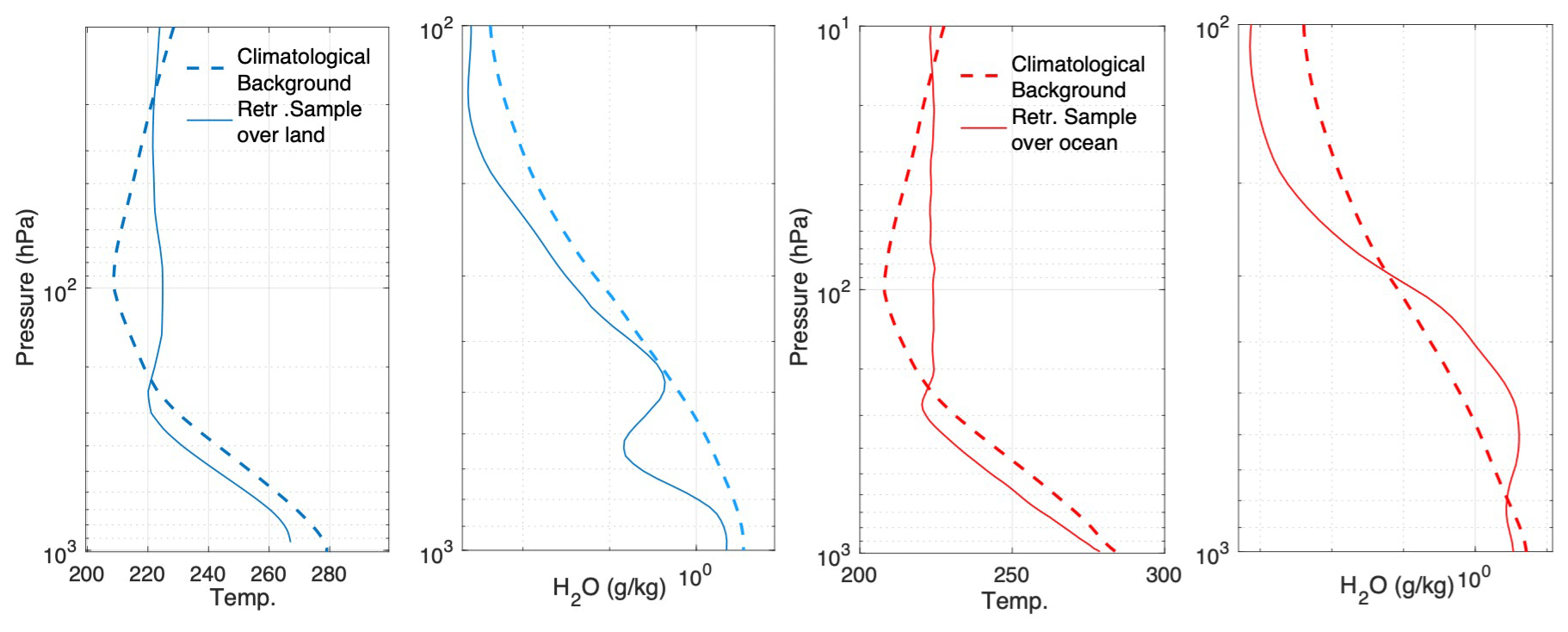
Figure 1 Climatological background used for temperature and water vapor retrievals (dash curves) in the SiFSAP algorithm. The final retrieval results (sample retrieved profiles presented as solid curves) can be very different from the background values.

This paper gives a detailed introduction to the data content, the data-processing scheme, and the physical-retrieval methodology of SiFSAP. Validation of retrieval performance for SiFSAP key products is also presented.

2 Overview of the data content and the retrieval system

The SiFSAP system is designed to process data from major hyper-spectral sounders including AIRS, IASI, and CrIS. It can be easily extended to process future sounders like IASI-NG (New Generation) once the requisite PCRTM module is correspondingly updated. The system depends upon PCRTM's capability of simulating various hyper-spectral sounder measurements using a common forward-model module. Previous forward-model comparison studies have validated PCRTM's capability of simulating hyper-spectral sounder measurements with a high degree of radiometric fidelity (Aumann et al., 2018). Figure 2 demonstrates the use of SiFSAP to simulate sample TOA spectral radiances measured by three major hyper-spectral sounder instruments: IASI, CrIS, and AIRS. Benefiting from its modular design, the SiFSAP system is capable of using the collocated microwave (MW) observations to supplement IR retrievals under thick cloud conditions. Currently the SiFSAP system provides three retrieval schemes to meet different application needs based on the observation data availability: IR-only, MW-only, and IR+MW retrievals. The MW retrieval unit uses the Community Radiative Transfer Model (CRTM) to simulate the measurements by major MW sounders including the Advanced Technology Microwave Sounder (ATMS), the Advanced Microwave Sounding Unit (AMSU-A), and the Microwave Humidity Sounder (MHS). Details about CRTM can be found in the CRTM user's guide (Han et al., 2020) and its general introduction paper (Liu et al., 2012). SiFSAP products are generated using the synergistic IR+MW retrievals with IR and MW spectra being fitted simultaneously during the combined retrieval process. SiFSAP products include temperature, water vapor, and trace gas profiles at 98 pressure levels, surface skin temperature, IR surface emissivity at native mono-frequency bins defined by the PCRTM, MW surface emissivity for all MW sounder channels, effective cloud top pressure, cloud optical depth (at 550 nm), cloud particle size, and cloud liquid water content. Table 1 lists the major geophysical properties included in SiFSAP.

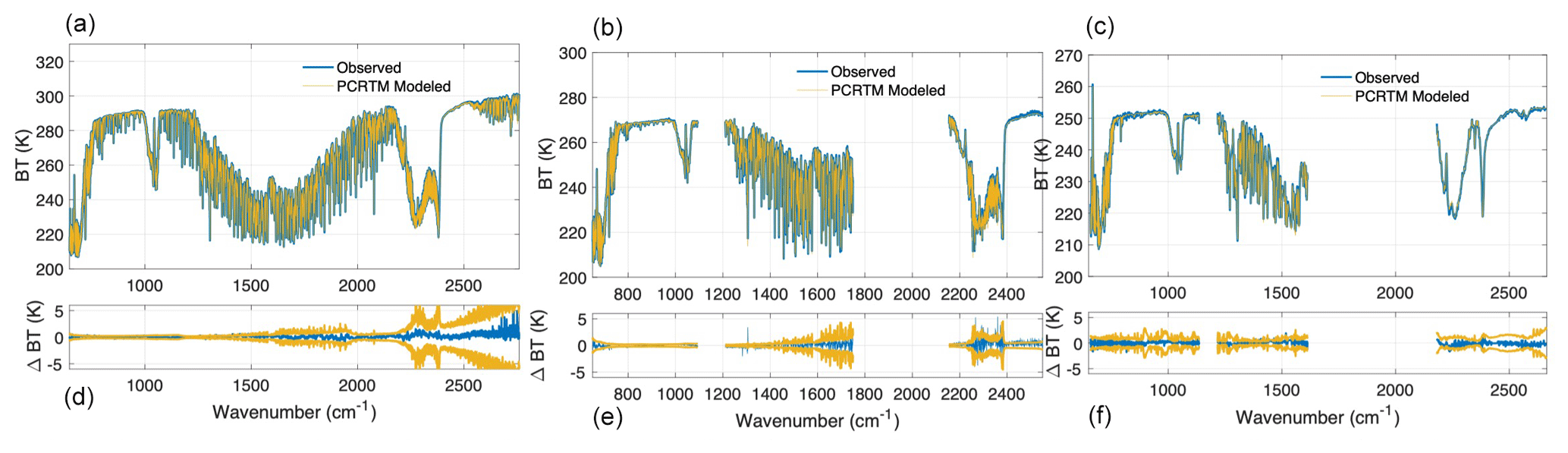
Figure 2 IR sounder radiances fitted by SiFSAP. (a) IASI; (b) CrIS; (c) AIRS. The radiance-fitting residues (blue curves in the lower panels) are compared with the instrumental random noise (with the magnitude being marked using yellow curves). BT: brightness temperature.

Table 1 Geophysical parameters included in SiFSAP. MMR: mass mixing ratio. VMR: volume mixing ratio.

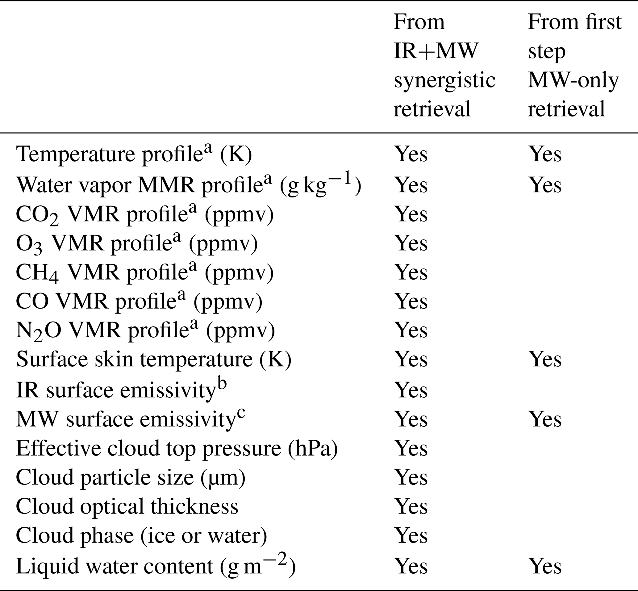
^a Atmospheric profiles are given at 98 pressure levels.
^b IR surface emissivity at native mono-frequency bins defined by the PCRTM is provided. The number of frequency bins for different sounders is as follows: 500 for AIRS, 753 for IASI, 540 for CrIS at full resolution, and 485 for CrIS at nominal resolution.
^c MW surface emissivity is given for each channel of MW sounders.

Figure 3 illustrates the flow diagram of the SiFSAP system. The SiFSAP processing starts with a pre-processor that loads the Level-1B data of the IR and MW sounders and the surface pressure values from the National Centers for Environmental Prediction (NCEP) Global Forecast System (GFS) model fields. The MW sounder data are spatially resampled to overlap with IR sounder observations of single FOVs via nearest-neighbor gridding. The GFS surface pressure data are interpolated in time and space to the IR sounder footprints. At the synergetic data-processing stage, the SiFSAP system includes three modular units: the initialization unit, the synergetic retrieval unit, and the post-processing unit. The initialization unit loads static databases including PCRTM and CRTM forward-model parameters, lookup tables (LUTs), climatological background fields, a priori covariance matrices, measurement uncertainties covariance matrices, and pre-trained spectral bias correction coefficients. The synergetic retrieval unit includes a two-step process: MW-only retrieval followed by IR+MW combined retrieval. The temperature, water vapor, and surface skin temperature from the first-step MW-only retrieval, once passing the MW radiance convergence test, are used as the first guess for the combined IR+MW retrieval. If the MW retrieval does not pass the first-step convergence test, the climatological first guess is used for the combined retrieval. If the geophysical properties retrieved for one FOV pass the quality control (QC), they are used as the first-guess values for the next FOV. Again, the climatological first guess will be used for the next FOV if the retrieval of the current FOV does not converge. The MW and the IR+MW combined retrieval results are passed to the QC and post-processing unit where QC flags are assigned, auxiliary data such as the tropopause height and the surface temperature are derived based on the retrieved atmospheric parameters, and the results are written to output files.

Figure 3 Flow diagram of the SiFSAP data-processing scheme.

3 Inversion methodology

3.1 Optimal estimation

Both the MW-only retrieval and the IR+MW combined retrieval are optimal-estimation-based physical-inversion processes. They are used to find the geophysical state vector x for a given measurement r with

$$\begin{array}{}\text{(1)}& \mathit{r}=F\left(\mathit{x}\right)+\mathit{ϵ},\end{array}$$

where F represents the radiative transfer forward model and ϵ represents the total error term that includes contributions from the measurement error, the forward-model error, and the representation error. A solution x is given by minimizing the cost function J, being defined as

$$\begin{array}{}\text{(2)}& \begin{array}{rl}J\left(\mathit{x}\right)& ={\left(\mathit{r}-F\left(\mathit{x}\right)\right)}^T{\mathbf{S}}_{\mathit{ϵ}}^{-\mathrm{1}}\left(\mathit{r}-F\left(\mathit{x}\right)\right)\\ & +{\left(\mathit{x}-{\mathit{x}}_{\mathrm{a}}\right)}^T{\mathbf{S}}_{\mathrm{a}}^{-\mathrm{1}}\left(\mathit{x}-{\mathit{x}}_{\mathrm{a}}\right),\end{array}\end{array}$$

where S_ϵ is the covariance of the error term ϵ. x_a and S_a are the background and covariance of a priori constraint in the domain of the geophysical state vector. The nonlinearity of the radiative transfer function defined in Eq. (1) requires an iterative minimization process to find a solution. Following the Gauss–Newton method suggested by Rodgers (2000), a solution can be given as

$$\begin{array}{}\text{(3)}& \begin{array}{rl}{\mathit{x}}_{n+\mathrm{1}}-{\mathit{x}}_n=& {\left({\mathbf{K}}^T{\mathbf{S}}_{\mathit{ϵ}}^{-\mathrm{1}}\mathbf{K}+{\mathbf{S}}_{\mathrm{a}}^{-\mathrm{1}}\right)}^{-\mathrm{1}}\\ & \left({\mathbf{K}}^T{\mathbf{S}}_{\mathit{ϵ}}^{-\mathrm{1}}\left(\mathit{r}-{\mathit{r}}_n\right)-{\mathbf{S}}_{\mathrm{a}}^{-\mathrm{1}}\left(\mathit{x}-{\mathit{x}}_{\mathrm{a}}\right)\right),\end{array}\end{array}$$

where K is the Jacobian, i.e., the first derivative which defines the sensitivity of the measurement to the input parameters:

$$\begin{array}{}\text{(4)}& \mathbf{K}={\left.{\displaystyle \frac{\mathrm{d}F\left(\mathit{x}\right)}{\mathrm{d}\mathit{x}}}\right|}_{\mathit{x}={\mathit{x}}_n}.\end{array}$$

The Gauss–Newton approach works well when the degree of nonlinearity is small. The step size of the iterative process must be optimally controlled to ensure it is still within the linear region. This is achieved in SiFSAP following the method described in Wu et al. (2017) and Lynch et al. (2009). The method uses the radiance residual between the observation and simulation at each step as a proxy to control the step size. Specifically, the solution is obtained by

$$\begin{array}{}\text{(5)}& \begin{array}{rl}{\mathit{x}}_{n+\mathrm{1}}-{\mathit{x}}_n=& {\left({\mathbf{K}}^T{\mathbf{S}}_{\mathrm{r}}^{-\mathrm{1}}\mathbf{K}+{\mathbf{S}}_{\mathrm{a}}^{-\mathrm{1}}\right)}^{-\mathrm{1}}\\ & \left({\mathbf{K}}^T{\mathbf{S}}_{\mathrm{r}}^{-\mathrm{1}}\left(\mathit{r}-{\mathit{r}}_n\right)-{\mathbf{S}}_{\mathrm{a}}^{-\mathrm{1}}\left(\mathit{x}-{\mathit{x}}_{\mathrm{a}}\right)\right).\end{array}\end{array}$$

S_r provides the constraint in the measurement domain that is adjusted during each step of the minimization approach. The inversion is known to be an ill-posed problem. The dimension reduction in the inversion matrix is usually needed to stabilize the solution and reduce the computational cost. The dimension reduction can be done in both the measurement vector r and the geophysical state vector x domain. While MW sounders have a limited number of channels (AMSU – 15 channels; MHS – 5 channels; ATMS – 22 channels), the dimension reduction is critical to process information from hyper-spectral IR sounders' thousands of spectral channels. In NUCAPS, CHART, and CLIMCAPS, only a few hundred selected IR channels are used for the retrieval (due to processing constraints in forward-model and inverse-model calculations). In SiFSAP, the synergetic measurement vector r for the IR+MW retrieval consists of the principal component (PC) scores of IR radiances and the channel brightness temperatures (BTs) of MW measurements:

$$\begin{array}{}\text{(6)}& \mathit{r}=\left[p_{\mathrm{1}}\mathrm{\dots }{p}_{N_{\mathrm{ir}}},r_{\mathrm{1}}\mathrm{\dots }{r}_{N_{\mathrm{mw}}}\right],\end{array}$$

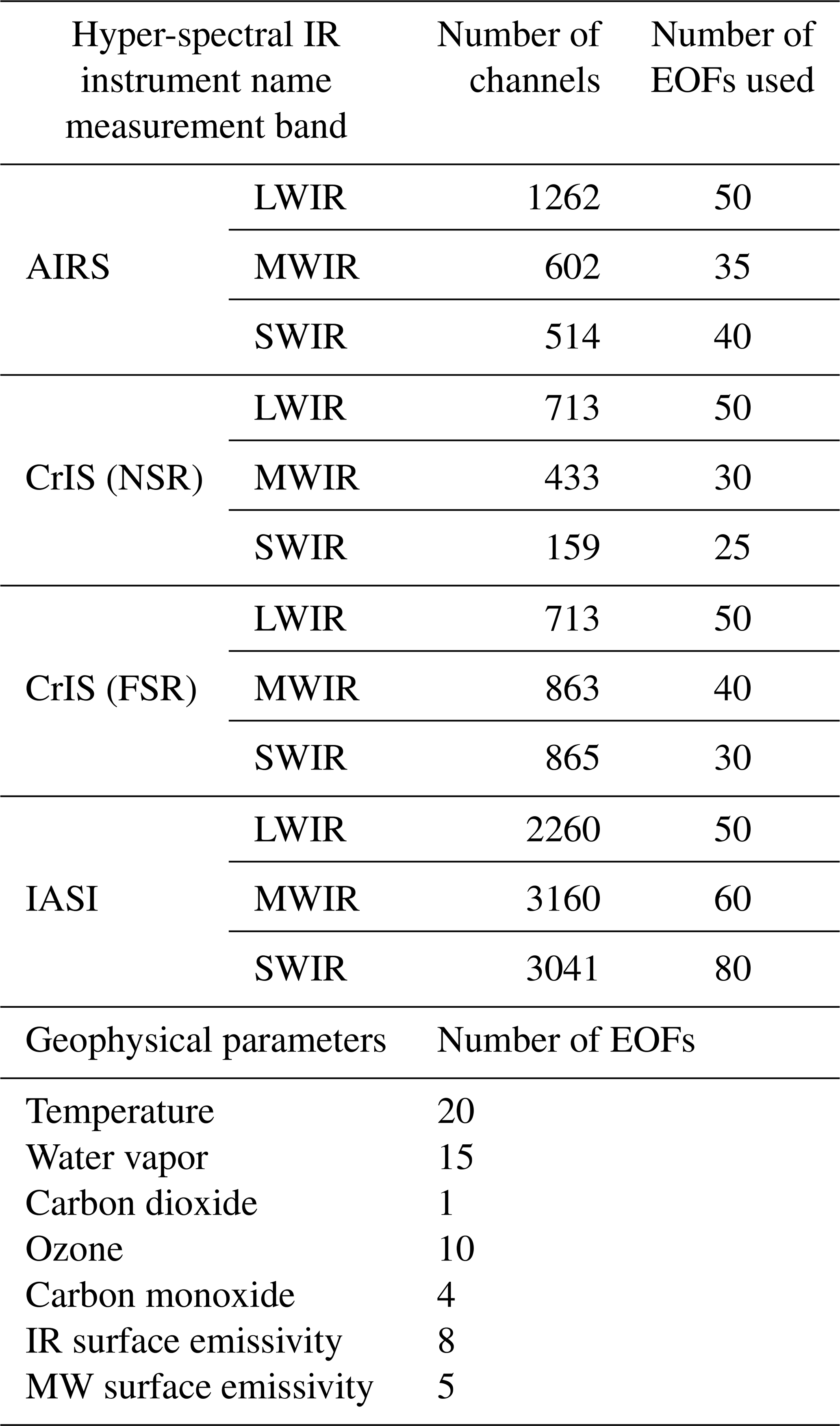
where p denotes the PC scores of IR radiances with N_ir being the total number of EOFs used and r_i denotes the MW BTs of N_mw channels. The use of PC representation allows us to use all spectral channels of IR sensors and filter out instrument random noise. The solution x includes all retrieved parameters that are used to quantify atmospheric vertical profiles, cloud information, and surface properties in the SiFSAP system. The dimension of the state vector x also needs to be limited to reduce the computational cost and ensure the numerical stability. For example, atmospheric vertical profiles are usually not directly represented as level (or layer) quantities on a high-vertical-resolution pressure grid in a retrieval system. Retrieval algorithms including NUCAPS, CHART, and CLIMCAPS use a linear combination of pre-defined trapezoidal functions to represent vertical profiles. The principal component (PC) analysis is used to reduce the dimension of the geophysical state vector x in SiFSAP. Atmospheric profiles and surface emissivity spectra are projected onto a set of pre-computed EOFs. Table 2 lists the dimension of measurement and geophysical state vectors used in SiFSAP. Both the IR+MW and MW-only retrieval follow the same minimization scheme to find the solution of x in the EOF domain. The dimensions of r, S_r, and K are 1×N_mw, N_mw×N_mw, and N_mw×N_x for the first-stage MW-only retrieval and $\mathrm{1}\times \left(N_{\mathrm{mw}}+N_{\mathrm{ir}}\right)$, $\left(N_{\mathrm{mw}}+N_{\mathrm{ir}}\right)\times \left(N_{\mathrm{mw}}+N_{\mathrm{ir}}\right)$, and $\left(N_{\mathrm{mw}}+N_{\mathrm{ir}}\right)\times N_x$ for the second-stage IR+MW combined retrieval. Here N_x is the length of the geophysical state vector x.

Table 2 Number of EOFs used in SiFSAP to represent radiances and geophysical parameters. SWIR: shortwave infrared. LWIR: longwave infrared. MWIR: midwave infrared. FSR: full spectral resolution.

Averaging kernels for retrieved atmospheric profiles are provided in SiFSAP. The vertical resolution of the retrieved atmospheric temperature, moisture, and other trace gases can be characterized using the averaging kernel:

$$\begin{array}{}\text{(7)}& \mathbf{A}={\left({\mathbf{K}}^T{\mathbf{S}}_{\mathrm{r}}^{-\mathrm{1}}\mathbf{K}+{\mathbf{S}}_{\mathrm{a}}^{-\mathrm{1}}\right)}^{-\mathrm{1}}{\mathbf{K}}^T{\mathbf{S}}_{\mathrm{r}}^{-\mathrm{1}}\mathbf{K}.\end{array}$$

Averaging kernels are also used to derive the degree-of-freedom (DOF) metric of the signal,

$$\begin{array}{}\text{(8)}& d_{\mathrm{s}}=\text{tr}\left(\mathbf{A}\right),\end{array}$$

a scalar used to evaluate the vertical information content provided by the measurements. Error estimations for each retrieved variable are also included in SiFSAP output. Following the definition by Rodgers (1990), we calculate the total retrieval error covariance matrices:

$$\begin{array}{}\text{(9)}& {\mathbf{S}}_x={\left({\mathbf{K}}^T{\mathbf{S}}_{\mathrm{r}}^{-\mathrm{1}}\mathbf{K}+{\mathbf{S}}_{\mathrm{a}}^{-\mathrm{1}}\right)}^{-\mathrm{1}}.\end{array}$$

All geophysical variables are simultaneously and directly retrieved in the SiFSAP scheme. This avoids the complicated characterization of error propagation needed in sequential retrieval algorithms, e.g., CLIMCAPS (Smith and Barnet, 2019). The direct retrieval of the state vector related to cloud properties also avoids the uncertainty introduced by “cloud clearing”, which is difficult to quantify and susceptible to the quality of the atmospheric state used to derive a clear-sky TOA spectrum for cloud clearing.

The overall QC flags are determined based on the cost function zeta (ζ) that characterizes how well the simulated radiance using a forward model fits the observed radiances. It is calculated as

$$\begin{array}{}\text{(10)}& \mathit{\zeta }={\left({\mathit{r}}^{\mathrm{simu}}-{\mathit{r}}^{\mathrm{obs}}\right)}^T{\mathbf{S}}_{\mathit{ϵ}}^{-\mathrm{1}}\left({\mathit{r}}^{\mathrm{simu}}-{\mathit{r}}^{\mathrm{obs}}\right).\end{array}$$

The ζ threshold values for MW-only and IR+MW retrievals are empirically assigned to achieve an optimized balance between retrieval accuracy and yield rate. The ζ values for the retrieval of trace gas species are calculated using the selected IR sounder channels in the corresponding absorption regions.

3.2 A priori constraint and representation of geophysical variables

A priori constraints are best used in the retrieval to supplement the information that cannot be provided by the measurements. Depending on the information content that can be obtained from IR or MW sounder data, different a priori constraints are used for different retrieval variables. Climatological backgrounds and error covariances used for temperature and water vapor retrieval in the SiFSAP system are derived from a combined dataset with more than 30 000 globally distributed atmospheric profiles (Liu et al., 2009; Wu et al., 2017). These profiles include European Centre for Medium-Range Weather Forecasts (ECMWF) reanalysis data, radiosonde measurements, and satellite-based observations. The atmospheric profiles are represented by level quantities on a grid of 98 pressure levels from the surface to TOA in the retrieval system. The EOFs corresponding to the temperature and water vapor state vectors are derived from the background error covariance matrices. The surface level index, which is determined by the surface pressure value, can be quite different for different land regions while remaining relatively constant over ocean. Therefore, EOFs and a priori constraints of temperature and water vapor are constructed as over-land and over-ocean groups. A conventional EOF transformation is used to represent temperature profiles in the form of

$$\begin{array}{}\text{(11)}& X_i^{\mathrm{Temp}}={\sum }_{j=\mathrm{1}}^{\mathrm{98}}{U}_{i,j}^{\mathrm{Temp}}\cdot \left(P_j^{\mathrm{Temp}}-\stackrel{\mathrm{‾}}{P^{\mathrm{Temp}}}\right),\end{array}$$

where X_i represents the ith EOF coefficient of a corresponding temperature profile P, which has an unit of Kelvin, with the climatological background $\stackrel{\mathrm{‾}}{P}$ being given as the mean value of the profiles included in generating the covariance matrix, and U_i is the ith significant eigenvector. The water vapor EOFs are built as the logarithm of water vapor profiles:

$$\begin{array}{}\text{(12)}& X_i^{{\mathrm{H}}_{\mathrm{2}}\mathrm{O}}={\sum }_{j=\mathrm{1}}^{\mathrm{98}}{U}_{i,j}^{{\mathrm{H}}_{\mathrm{2}}\mathrm{O}}\cdot \left(\log \left(P_j^{{\mathrm{H}}_{\mathrm{2}}\mathrm{O}}\right)-\stackrel{\mathrm{‾}}{\log \left(P^{{\mathrm{H}}_{\mathrm{2}}\mathrm{O}}\right)}\right).\end{array}$$

EOFs of ozone profiles are also constructed using globally distributed data but separated as over-land and over-ocean groups, similar to temperature and water vapor. The absolute value of ozone concentration in the tropospheric region is very small compared with that in the stratospheric region. In order to better represent the variational feature of ozone profiles in the tropospheric region, the ozone EOFs are built as functions of the square root of ozone profiles:

$$\begin{array}{}\text{(13)}& X_i^{{\mathrm{O}}_{\mathrm{3}}}={\sum }_{j=\mathrm{1}}^{\mathrm{98}}{U}_{i,j}^{{\mathrm{O}}_{\mathrm{3}}}\cdot \left(\sqrt{P_j^{{\mathrm{O}}_{\mathrm{3}}}}-\stackrel{\mathrm{‾}}{\sqrt{P^{{\mathrm{O}}_{\mathrm{3}}}}}\right).\end{array}$$

Moreover, a priori constraints for ozone retrieval are stratified according to latitude and tropopause height to better constrain the retrieval in the regions where the ozone signal is weak. A priori constraints for ozone are generated using a synergistic dataset that combines data from the Model for OZone and Related chemical Tracers (MOZART), ozonesonde measurements, the European Centre for Medium-Range Weather Forecasts (ECMWF) analysis, and the Modern-Era Retrospective analysis for Research and Applications (MERRA). The synergistic dataset includes more than 400 000 ozone profiles and collocated temperature profiles. Those profiles are globally distributed and provide adequate coverage for seasonal variabilities. The ozone and temperature profiles are binned into eighteen 10^∘ latitudinal zones with each zonal group being further stratified into 13 tropopause-dependent subgroups. The tropopause height values are derived as the lowest level at which the temperature lapse rate decreases to 2 K km⁻¹ or less. To further cover the seasonal variation characteristics of the ozone climatology, a linear regression relationship between the ozone profiles and the collocated temperature profiles are derived for each latitude–tropopause subgroup. The a priori covariance of each subgroup is derived as the regression-prediction uncertainty using the temperature and ozone data and saved as a static database. With a given tropopause height and a latitude, an individual retrieval is first assigned to a subgroup so that the a priori covariance to be used in the SiFSAP system can be directly loaded. The first-guess values used for the ozone retrieval are obtained using the pre-established regression relationship of the assigned subgroup and the temperature profiles from the first-step MW retrieval. The SiFSAP system provides the option of using either the tropopause height from the real-time forecast data provided by National Centers for Environmental Prediction (NCEP) or that derived using temperature profiles from the first-step MW retrieval. Both options are well suited for near-real-time applications. The latitude-referenced ozone climatology has been adopted as in CHART (Susskind and Blaisdell, 2017) and NUCAPS (Barnet et al., 2021), while the tropopause-referenced ozone climatology is also used for ozone retrieval studies using AIRS measurements (Wei et al., 2010) as well as the planned measurements of the Tropospheric Emissions: Monitoring of Pollution (TEMPO) satellite (Johnson et al., 2018; Yang and Liu, 2019). The combined latitude–tropopause information provides a quality estimate of the ozone variability that changes latitudinally and correlates with the synoptic-scale meteorological features of the tropopause.

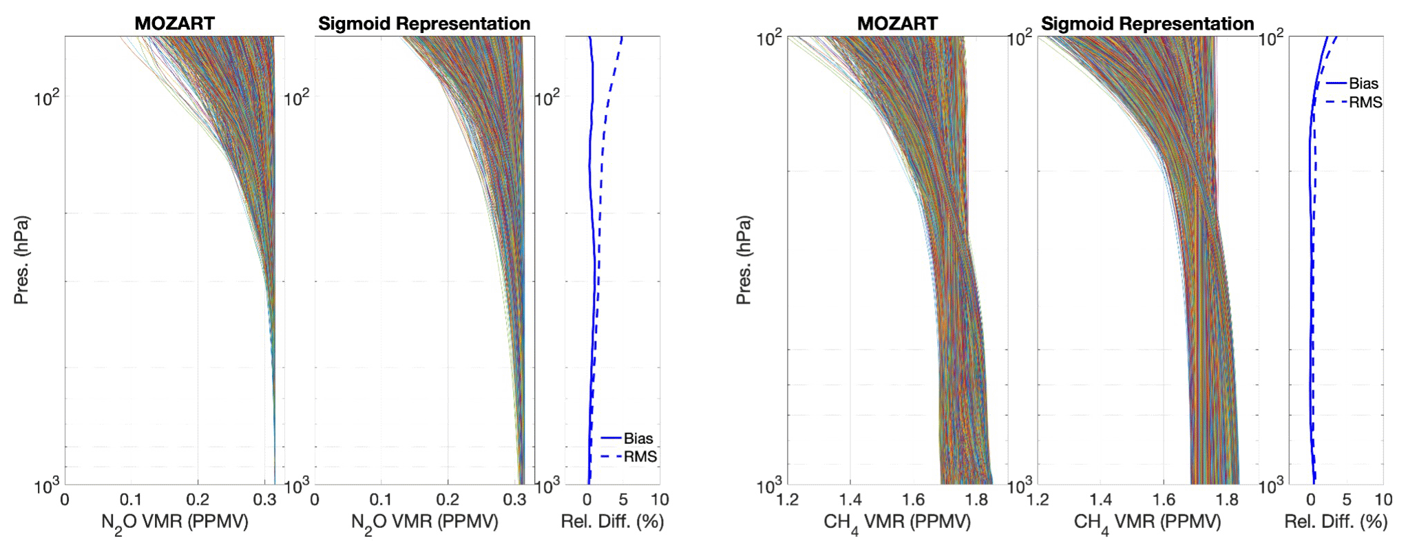
Carbon monoxide (CO) EOFs are also built on the logarithm of profiles. Carbon dioxide is retrieved as averaged column density values. Methane (CH₄) and nitrous oxide (N₂O) are similar in the way that their concentrations are relatively stable below the tropopause and decrease with height via various chemical processes in the stratosphere. Since CH₄ and N₂O are well mixed in the troposphere and their mixing ratios decrease dramatically above the tropopause due to chemical reactions and photolysis, their ratio profiles (P) can be represented as a sigmoid-like function of altitude h to a good approximation:

$$\begin{array}{}\text{(14)}& P\left(h\right)={\displaystyle \frac{P_{\mathrm{0}}}{\mathrm{1}+e^{-\left(\frac{h-h_{\mathrm{0}}}{a_{\mathrm{0}}}\right)}}},\end{array}$$

where P₀ defines the near-surface mixing ratio, h₀ defines the dependence of vertical profiles on tropopause height, and a₀ determines the rate of decrement in the stratosphere. In this way, the retrieval of CH₄ and N₂O profiles is constrained to a solution defined by three parameters. The atmospheric distributions of CH₄ and N₂O are rather uniform zonally but exhibit a gradient with latitude. P₀, h₀, and a₀ values for given individual profiles are obtained by fitting the vertical profiles according to the function defined by Eq. (14). The first-guess values and the corresponding covariance constraints for P₀, h₀, and a₀ are statistically obtained using a MOZART database that includes globally distributed CH₄ and N₂O vertical profiles of 12 different months. They are further stratified into 18×13 latitude–tropopause-dependent groups. This is similar to the strategy adopted to construct the ozone a priori constraint, except that there is a lack of correlation between CH₄ or N₂O profiles and the collocated temperature profiles so that the mean values of specified groups are used as the first-guess values instead. The first guess of the surface mixing ratio P₀ for each individual retrieval is further adjusted according to the globally averaged, monthly mean atmospheric methane and nitrous oxide concentration determined from the observation network of various air-sampling sites whose locations range in latitude from 90^∘ S to 82^∘ N (Dlugokencky et al., 1994).

The EOFs for MW surface emissivity over ocean are built from simulated emissivity spectra using the Wilheit (1979) model and an improved fast microwave water emissivity model, FASTEM (Liu et al., 2011). The Masuda model (Masuda et al., 1988) and surface-leaving radiance model (Nalli et al., 2008a, b) are used for the simulation of IR surface emissivity samples over ocean. The simulations use randomly generated wind speed and surface temperature data within a realistic dynamic range. The EOFs for MW land emissivity spectra are obtained using English's semi-empirical model (Hewison and English, 1999). The EOFs for IR land surface emissivity are constructed using data from the ECOsystem Spaceborne Thermal Radiometer Experiment on Space Station (ECOSTRESS) spectral emissivity databases (Meerdink et al., 2019; Baldridge et al., 2009). For both MW and IR retrievals, the surface emissivity function

$$\begin{array}{}\text{(15)}& F\left(\mathit{\epsilon }\right)=\log \left(\log \left({\displaystyle \frac{{\mathit{\epsilon }}_{max}-\mathit{\epsilon }}{{\mathit{\epsilon }}_{max}-{\mathit{\epsilon }}_{min}}}\right)\right)\end{array}$$

is introduced to constrain the retrieved surface emissivity within a range between ε_max and ε_min, which are empirically based on the best knowledge of surface emissivity (Zhou et al., 2010).

Figures 4–6 demonstrate the representation of sample temperature, water vapor, ozone and carbon monoxide profiles using different numbers of EOFs as specified in Table 2. The temperature and water vapor profile samples used for the validation are from selected ECMWF reanalysis profiles. Ozone and carbon monoxide profiles are randomly selected from the synthesized datasets used to build a priori constraints for the retrieval, including data from sonde measurements, reanalysis databases, and geochemical-model results. Along with the plots that illustrate the distribution of true profiles, the EOF representation errors are quantified in terms of their mean bias and root mean square (rms) values. Figure 7 demonstrates the representation of sample N₂O and CH₄ vertical profiles from MOZART using the sigmoid representation functions.

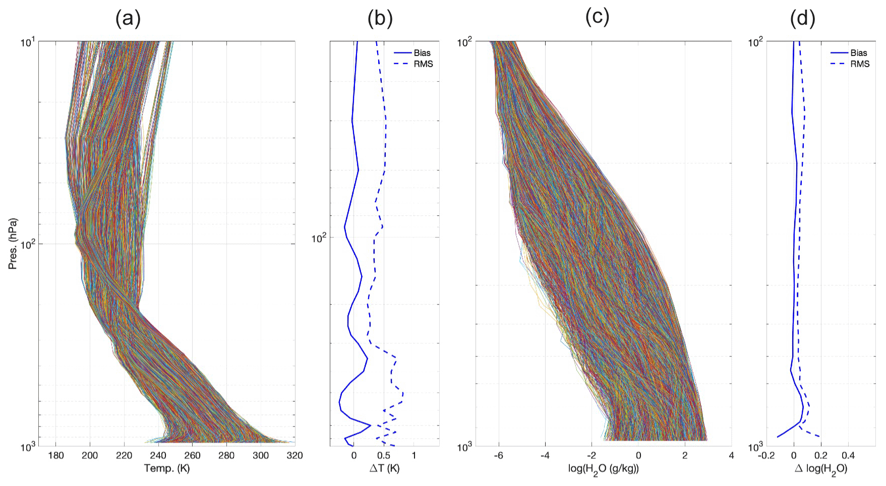
Figure 4 EOF representation errors in temperature and water vapor profiles. (a, c) Original temperature and water vapor profiles; (b, d) the mean and the rms values for the difference between the original profiles and the profiles being represented using a limited number of EOFs (20 EOFs are used for temperature profiles and 15 EOFs are used for water vapor).

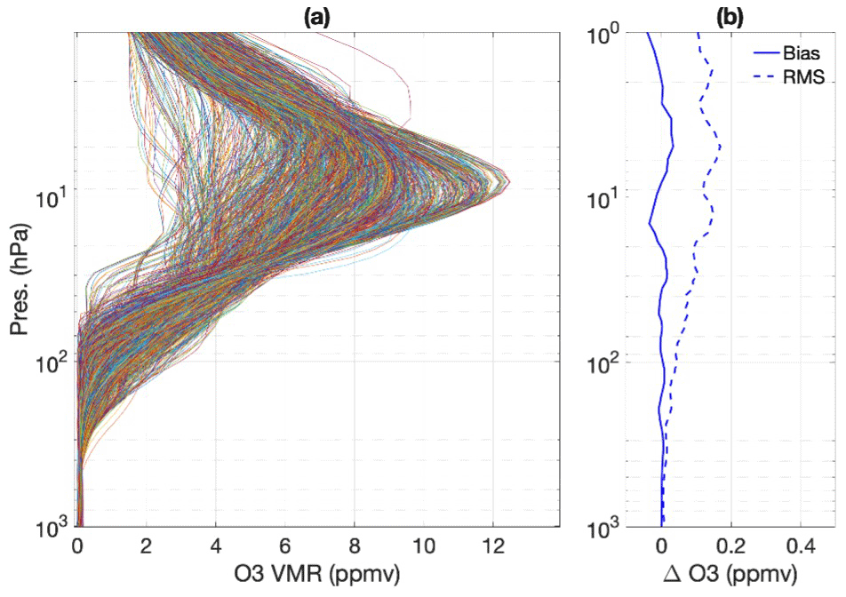
Figure 5 EOF representation errors in ozone profiles. (a) The original ozone profiles; (b) the mean and the rms values for the difference between the original profiles and the profiles being represented using 10 EOFs.

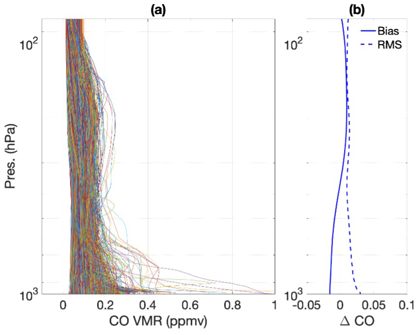
Figure 6 EOF representation errors in carbon monoxide profiles. (a) The original ozone profiles; (b) the mean and the rms values for the difference between the original profiles and the profiles being represented using four EOFs.

Figure 7 The representation of nitrous oxide and methane profiles using sigmoid functions.

3.3 Bias correction

As compared with the traditional IR+MW algorithms that rely on cloud clearing, the SiFSAP algorithm fits the TOA radiance directly and maximizes the contribution from the measurement-provided information. The accuracy of the retrieval critically depends on how well the forward-model errors are addressed. The correction for forward-model errors (here referred as “bias correction”) in the SiFSAP scheme includes two parts: (1) the correction for the channel brightness temperatures of MW sounder measurements and (2) the correction for the hyper-spectral measurements of IR sounders. Forward-model errors, which can be generalized as the difference between the simulated radiance and the observations, may arise from the spectroscopy inaccuracies and/or the fast parameterizations used in the radiative transfer models. In an optimal-estimation-based retrieval scheme, forward-model errors can be corrected by subtracting the systematic bias (the mean value of ϵ defined in Eq. 1) from the observation and accommodating the uncertainty in the error covariance of radiance residuals after the subtraction (S_ϵ defined in Eq. 6).

Estimation of the systematic bias and the error covariance is done by comparing the observations with radiances computed by the forward models using the best estimate of the truth as inputs. A common practice is to use the reanalysis data which are spatiotemporally matched to the selected ensemble of satellite observations as the truth of inputs. Data from the ECMWF reanalysis have been used to evaluate the simulation of MW sounders like ATMS (Zhou and Grassotti, 2020) and MHS (Schulte and Kummerow, 2019). Aumann et al. (2018) used ECMWF data to evaluate the simulation of hyper-spectral sounder measurements under cloudy-sky conditions using various radiative transfer models (RTMs) with cloud-scattering simulation capability, including PCRTM. All RTMs fit reasonably well in the 11 µm atmospheric window area. PCRTM has the smallest bias among the six RTMs for the cloudy-sky observations at 900 cm⁻¹ and provides the best match with observed AIRS radiances in the shortwave IR spectral region where the solar scattering of clouds is important.

MW sounder measurements are known to have systematic, scan-angle-dependent errors due to effects of antenna side lobes not being adequately accounted for in the calibration process. The differences between measured and computed spectra are usually scene dependent. Therefore, dynamic bias correction schemes for MW measurements have been implemented in the numerical weather prediction (NWP) data assimilation (DA) systems (Zhu et al., 2014; Dee and Uppala, 2009) and the physical-retrieval systems (Schulte and Kummerow, 2019). The dynamic bias correction schemes rely on the pre-trained relationship, being either a regression-based linear or a neural-network-based nonlinear scheme between the radiance bias and the predictors. The predictors include satellite angles and atmospheric and surface properties collocated with observations. Zhou and Grassotti (2020) studied the use of the ATMS brightness temperature (BT) as the major predictor in the Microwave Integrated Retrieval System (MiRS; https://www.star.nesdis.noaa.gov/mirs, last access: 20 February 2020). BTs are used along with other observation-angle- and scene-dependent predictors including latitude, cloud liquid water, total precipitable water, and surface skin temperature in the bias correction scheme. In the SiFSAP scheme, the MW bias corrections are stratified for different scan angles. Considering that the information about atmospheric and surface properties is already embedded in MW spectra, we choose the MW spectra as the only predictor in order to facilitate the operation of the SiFSAP algorithm, especially for near-real-time data production. The bias prediction used for the MW sounder is implemented through the following equation:

$$\begin{array}{}\text{(16)}& {\mathit{ϵ}}_j^{\mathit{\theta }}={\sum }_{i=\mathrm{1}}^{N_{\mathrm{mw}}}{A}_{ji}^{\mathit{\theta }}{R}_i^{\mathit{\theta }},\end{array}$$

where j and i are MW sounder channel index numbers, ${\mathit{ϵ}}_j^{\mathit{\theta }}$ is the scan-angle-dependent bias in the brightness temperature of MW sounder channel j, $A_{ji}^{\mathit{\theta }}$ is the regression-prediction coefficient that links the bias to the MW channel measurement $R_i^{\mathit{\theta }}$, and $A_{ji}^{\mathit{\theta }}$ is trained using the least-squares fit on the training sample. The matchup training samples of ϵ^θ and R^θ are constructed using collocated ECMWF data and MW sounder measurements from selected “focus” days. The ECMWF does not provide surface emissivity and accurate cloud information. Therefore, emissivity is tuned along with cloud properties within the constraint defined by the preconstructed a priori constraint. The solutions that provide the best match to the observations are selected. The difference between R^θ and the corresponding fitted radiances (in BT) is the bias ϵ^θ. We filter out the outliers of the matchup samples where the absolute differences between the simulated MW brightness temperatures using reanalysis data and the observed ones are greater than a predetermined threshold. Figure 8 illustrates the scan-angle-dependent bias of ATMS measurements on board the Suomi National Polar-orbiting Partnership (SNPP) and NOAA-20 satellites, respectively. Figures 9 and 10 further demonstrate the probability density distribution of the brightness temperature difference between the observations and the simulations for different ATMS channels. Figures 9 and 10 also show that the scene-dependent biases can be effectively corrected using the regression-prediction scheme. It is noted here that the global-mean daily biases from the simulation cannot be characterized as static offsets. The magnitudes of those offsets for different days can be very different and therefore cannot be effectively corrected via a static-offset subtraction.

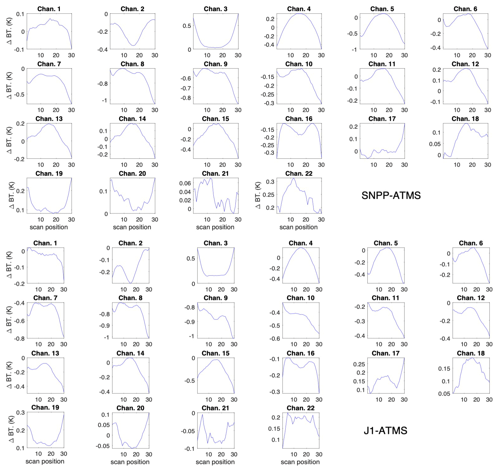
Figure 8 Global-mean bias (in BTs) predicted by the SiFSAP algorithm for ATMS measurements on board SNPP and NOAA-20 (JPSS-1, J1; Joint Polar Satellite System) on 30 April 2020.

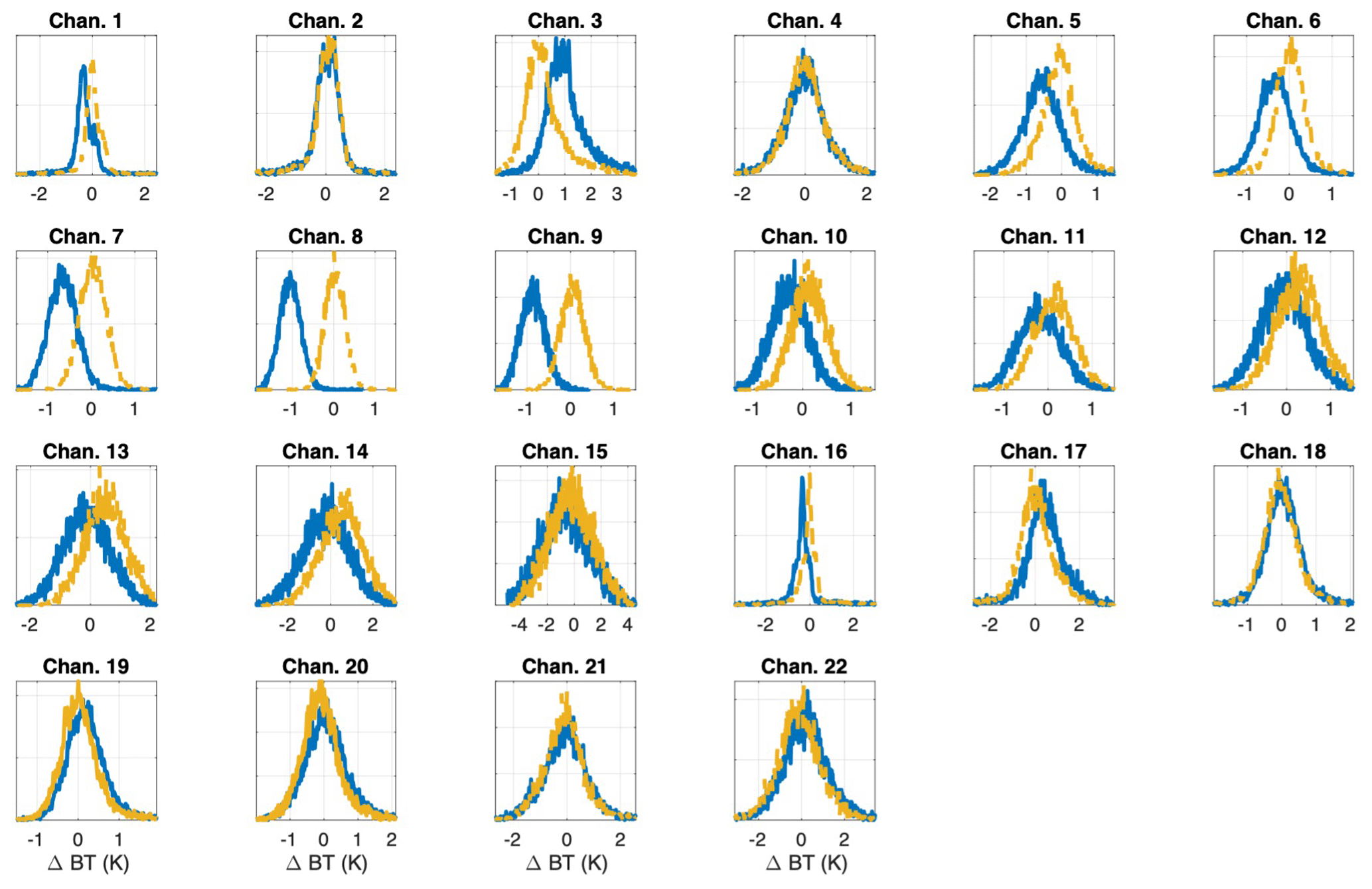
Figure 9 Solid blue curves: histograms that illustrate the distribution of biases in different SNPP ATMS channels for over-land measurements on 30 April 2020 at the 52.725^∘ scan position, derived from the study discussed in Sect. 3.3; dashed yellow curves: histograms of biases after the correction following the regression-prediction scheme.

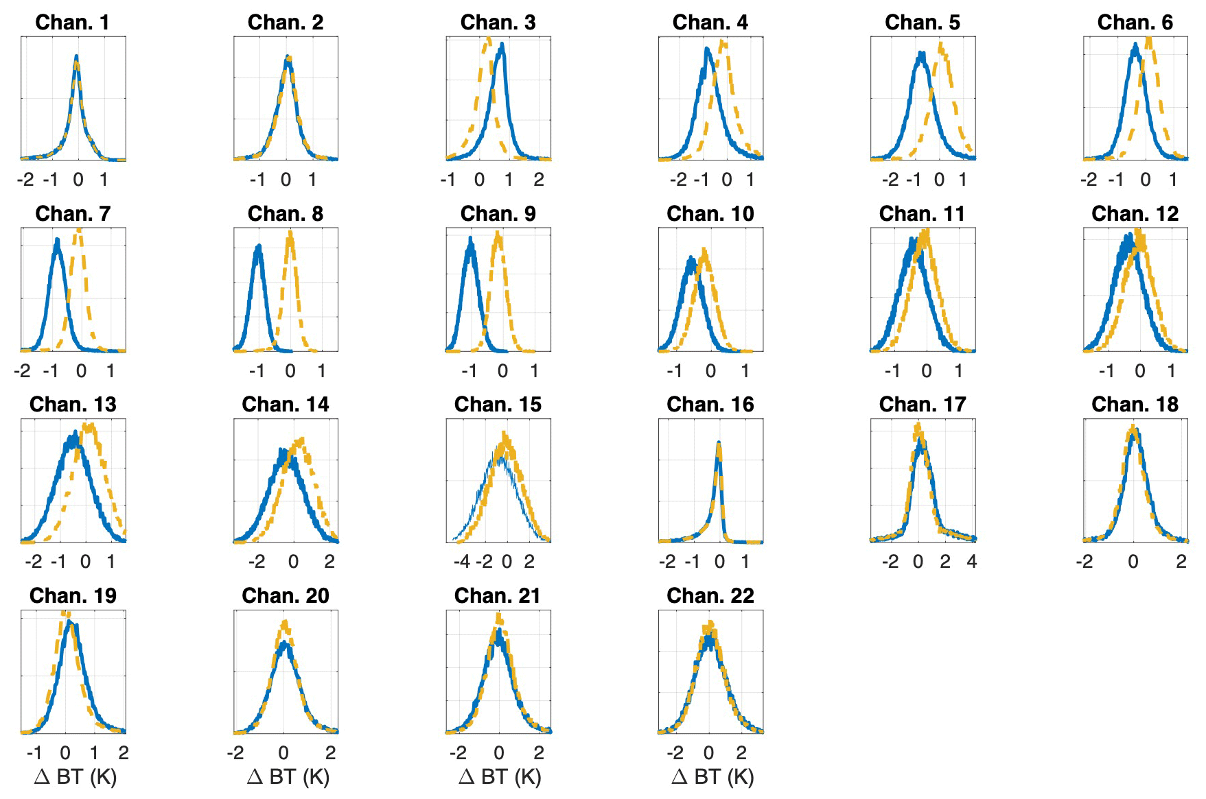
Figure 10 Blue curves: similar to Fig. 9 but for histograms that illustrate the distributions of biases in different NOAA-20 ATMS channels for over-ocean measurements at the 52.725^∘ scan position; dashed yellow curves: histograms of biases after the correction following the regression-prediction scheme.

The bias correction for the IR hyper-spectral retrieval follows a regression-prediction approach similar to that for the MW retrieval. IR sounder measurements do not have antenna-related, scan-angle-dependent errors so that a unified bias correction is used for measurements at all satellite scan angles:

$$\begin{array}{}\text{(17)}& {\mathit{ϵ}}_j={\sum }_{i=\mathrm{1}}^{N_{\mathrm{eof}}}{A}_{ji}{R}_i.\end{array}$$

Here both the bias and radiances are represented in the EOF domain. N_eof is the number of EOFs used to represent the hyper-spectral sounder radiances. Again, we need to fit surface spectral emissivity and cloud properties to minimize the differences between the simulated spectral radiances and the corresponding sample observations. The static bias correction term ϵ_j is small. What is critical here is the magnitude and the distribution of spectral-fitting residuals, which define the error covariance used for the retrieval (S_ϵ in Eq. 2). Figure 11 plots the spectral error covariance used for the SNPP CrIS retrieval.

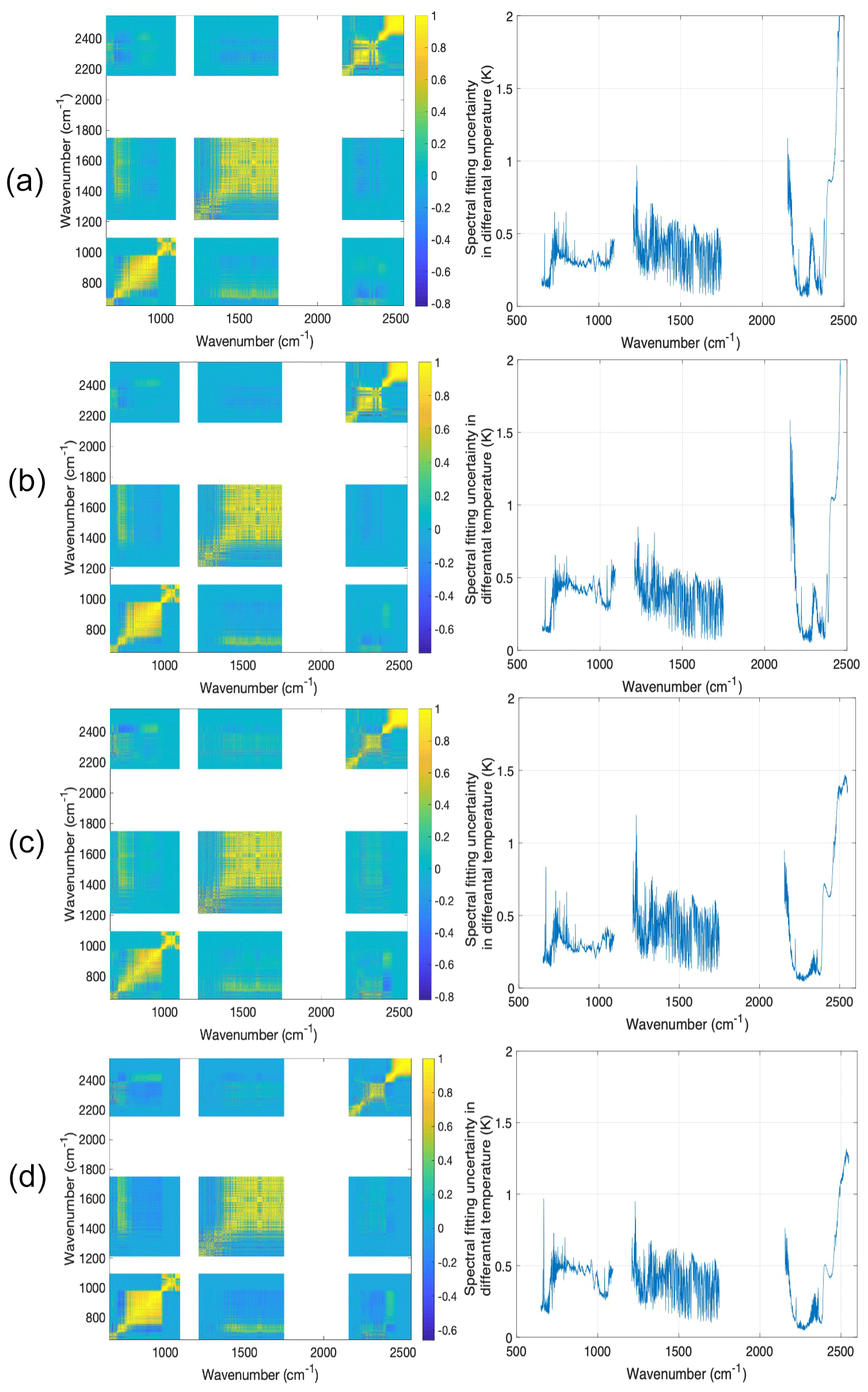
Figure 11 Left column: spectral-fitting error covariances (normalized by diagonal elements) used for the SNPP CrIS SiFSAP algorithm; right column: corresponding magnitude of the spectral-fitting uncertainty for each CrIS channel (quantified as differential temperature at 280 K) – (a) for over-ocean ascending observations, (b) for over-land ascending observations, (c) for over-ocean descending observations, and (d) for over-land descending observations.

4 Results and assessment

4.1 Radiance-fitting assessment

One important quality assessment factor for sounder retrieval products is how well the retrieved properties fit the radiance measurements. Providing the best fit to the measured TOA radiances is the first important indicator of the correct utilization of maximized information provided by the measurement. The capability of providing radiance “closure” justifies the retrieval products' application for climate monitoring. It is especially critical to ensure the traceable accuracy when the data from multiple sounder measurements like those from AIRS, CrIS, and IASI are fused together to establish a long-term climate data record (Strow et al., 2021; Wu et al., 2020). Figure 12 shows the global-mean spectral-fitting residuals between the CrIS radiances from SiFSAP and the observations for 14 January 2016. This daily mean fitting residual is derived using ∼ 90 % of CrIS single FOV measurements of that day. The capability of fitting the single FOV measurements under cloudy-sky conditions greatly facilitates the use of SiFSAP for climate studies that requires high-spatial-resolution and all-sky sampling.

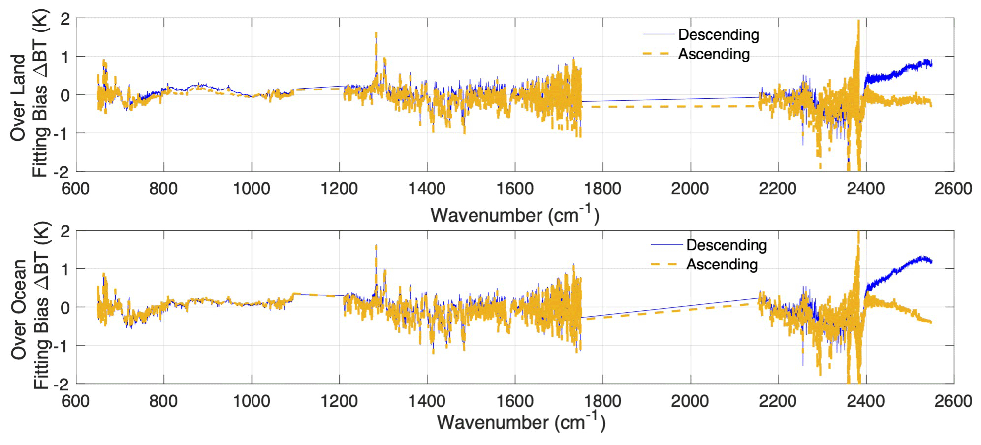
Figure 12 Global-scale daily mean spectral-fitting bias achieved by SiFSAP for SNPP CrIS observations on 14 January 2016.

4.2 Temperature and water vapor profiles

The validation of temperature and water vapor profiles from SiFSAP has been done using results from selected testing days. Figures 13 and 14 plot the global-mean and rms values of the differences between the temperature and the water vapor retrieved from SNPP CrIS–ATMS measurements during 16 July 2017 and those from the collocated ECMWF data. The bias and rms for the temperature difference are calculated as

$$\begin{array}{}\text{(18)}& \begin{array}{rl}& T_{\mathrm{Bias}}=\text{mean}\left(T_{\mathrm{SiFSAP}}-T_{\mathrm{ECMWF}}\right),\\ & T_{\mathrm{rms}}=\sqrt{\text{mean}\left({\left(T_{\mathrm{SiFSAP}}-T_{\mathrm{ECMWF}}\right)}^{\mathrm{2}}\right)}.\end{array}\end{array}$$

The bias and rms for the water vapor are calculated as

$$\begin{array}{}\text{(19)}& \begin{array}{rl}& {{\mathrm{H}}_{\mathrm{2}}\mathrm{O}}_{\mathrm{Bias}}={\displaystyle \frac{\text{mean}\left({{\mathrm{H}}_{\mathrm{2}}\mathrm{O}}_{\mathrm{SiFSAP}}-{{\mathrm{H}}_{\mathrm{2}}\mathrm{O}}_{\mathrm{ECMWF}}\right)}{\text{mean}\left({{\mathrm{H}}_{\mathrm{2}}\mathrm{O}}_{\mathrm{ECMWF}}\right)}}\times \mathrm{100}\mathit{\%},\\ & \mathrm{\text{rms}}={\displaystyle \frac{\sqrt{\text{mean}\left({\left({{\mathrm{H}}_{\mathrm{2}}\mathrm{O}}_{\mathrm{SiFSAP}}-{{\mathrm{H}}_{\mathrm{2}}\mathrm{O}}_{\mathrm{ECMWF}}\right)}^{\mathrm{2}}\right)}}{\text{mean}\left({{\mathrm{H}}_{\mathrm{2}}\mathrm{O}}_{\mathrm{ECMWF}}\right)}}\times \mathrm{100}\mathit{\%}.\end{array}\end{array}$$

We can see that above 10 km, temperature profiles from SiFSAP have a retrieval accuracy better than 1 K. The retrieval uncertainty becomes larger in the lower-troposphere region, mostly due to the limited sensitivity of IR sounders to atmospheric profiles below thick clouds. The retrieval accuracy for profiles below clouds becomes more dependent on the retrieval accuracy of the MW sounders as clouds get thicker. As compared with over-ocean retrievals, the relatively larger uncertainty in the land surface emissivity leads to a larger uncertainty in the near-surface temperature retrieval. The relative error in water vapor retrieval is around 20 % or smaller in the completely tropospheric region.

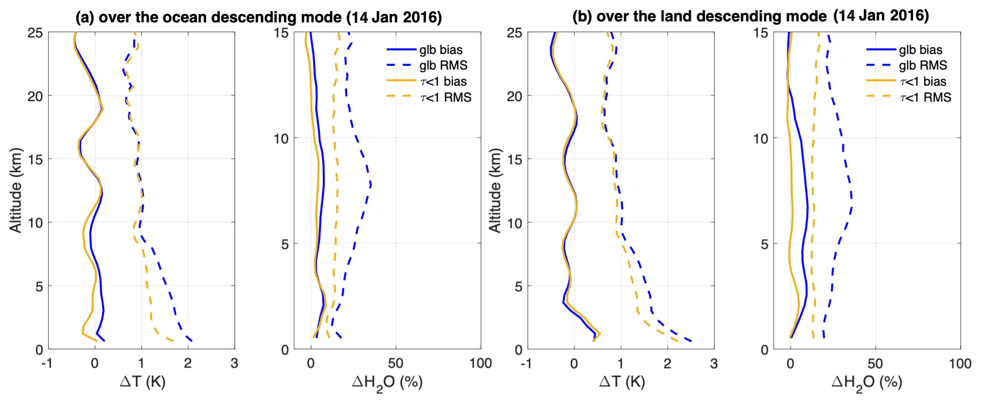
Figure 13 Error statistics of global (glb) temperature and water vapor profiles retrieved from SNPP CrIS–ATMS descending observations with respect to the ECMWF for (a) over-ocean scenes and (b) over-land scenes. Solid lines: biases of temperature and water vapor profiles; dashed lines: rms errors in the temperature and water vapor profiles. In addition to the bias and rms values for all CrIS–ATMS descending measurements, the statistics for observations under either a clear sky or thin clouds (cloud optical depth less than 1.0) are explicitly plotted to illustrate the impact of clouds on the retrieval accuracy of temperature and water vapor profiles at low altitudes.

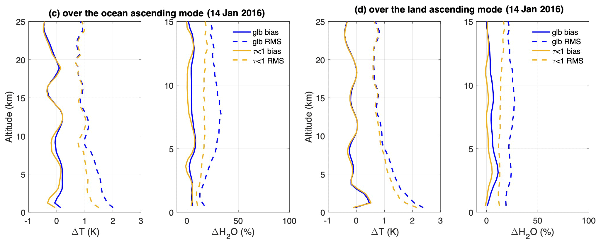
Figure 14 Error statistics of global (glb) temperature and water vapor profiles retrieved from SNPP CrIS–ATMS ascending observations with respect to the ECMWF for (c) over-ocean scenes and (d) over-land scenes.

4.3 Surface emissivity

Figure 15 demonstrates sample land surface emissivity spectra retrieved from CrIS observations over different areas with different surface conditions. We can clearly see the strong spectral feature in the quartz reststrahlen band between 8 and 10 µm (1000–1250 cm⁻¹) for samples in the desert and very different emissivity features for surfaces of soil and/or plants. Figure 16 compares the land surface emissivity at 11 µm of 2 selected days (14 January 2016 and 8 August 2017) with the Aqua MODIS daily emissivity from the MOD21 Land Surface Temperature and Emissivity product (Hulley et al., 2016). The difference between Fig. 16a2 and a1 illustrates the change in surface emissivity that reflects the seasonal change (January–August) of vegetation coverage. There is a clear correlation between the emissivity change and the vegetation coverage change shown in Fig. 16c1 and c2 as the normalized difference vegetation index (NDVI). The NDVI values are extracted from the MODIS/Terra Vegetation Indices Monthly L3 Global 0.05Deg CMG (Climate Modeling Grid) product (Didan and Huete, 2015). There is a noticeable emissivity difference between Fig. 16a1 and a2, which can partly be explained by the change in snow coverage in this area from January to August in 2016 (shown in Fig. 16d1 and d2). The snow coverage data are extracted from daily Level-3 (L3) MODIS Aqua snow coverage data products that provide the percentage of snow-covered land observed daily within 0.05^∘ (approx. 5 km) MODIS Climate Modeling Grid (CMG) cells (Hall and Riggs, 2021).

Figure 15 Sample land emissivity spectra from the SiFSAP algorithm for SNPP CrIS.

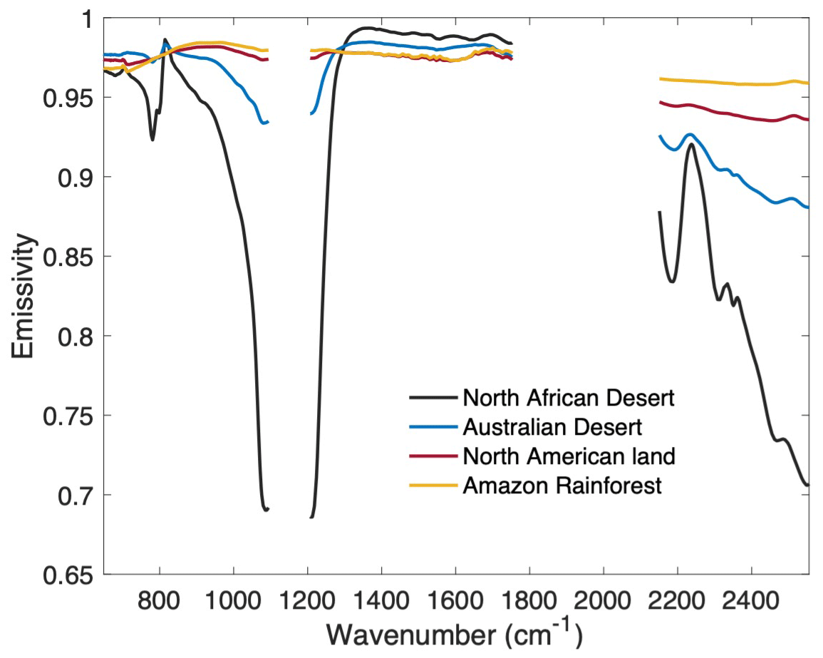
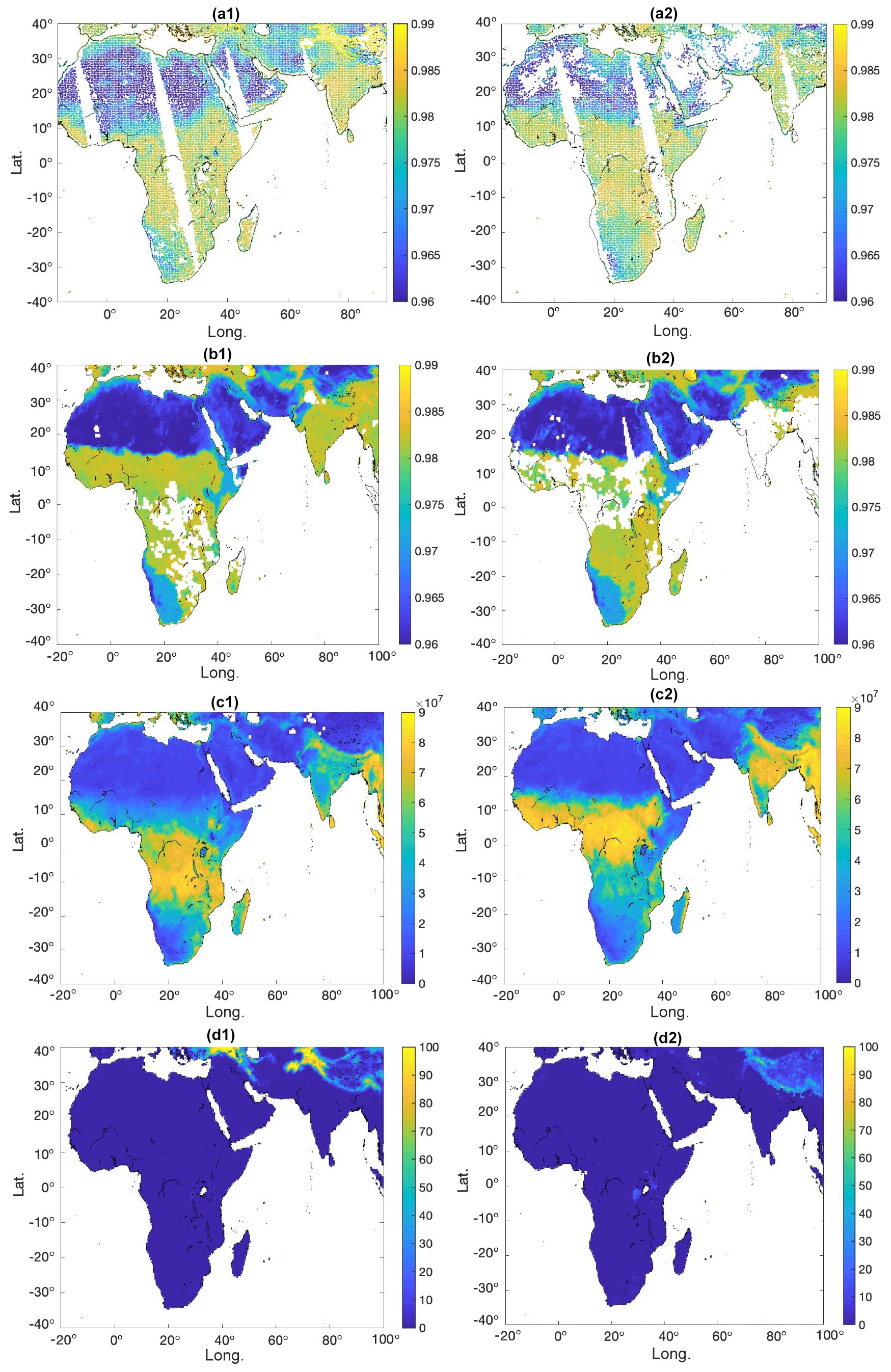
Figure 16 (a1, a2) SiFSAP surface emissivity at 11 µm for 14 January 2016 and 9 August 2017, respectively; (b1, b2) MODIS surface emissivity at 11 µm for January 2016 and August 2017, respectively; (c1, c2) MODIS monthly NDVI values for January 2016 and August 2017, respectively; (d1, d2) MODIS monthly snow coverage for January 2016 and August 2017, respectively. The area with relatively thicker clouds (cloud optical depth larger than 1.0) is filtered out in panels (a1) and (a2).

4.4 Trace gases: O₃, CO, CO₂, CH₄, and N₂O

The SiFSAP atmospheric composition products include the retrieved volume mixing ratio of CO₂, O₃, CO, CH₄, and N₂O at a grid of 98 vertical pressure levels defined by the PCRTM algorithm. SiFSAP products include trace gas profiles for each sounder FOV, i.e., matching the native spatial resolution of hyper-spectral sounder instruments. SiFSAP O₃ data have been used to study stratospheric intrusion (Xiong et al., 2022a) and cold-air outbreaks (Xiong et al., 2022b). SiFSAP CO data have been used for the process-oriented analysis of emission from large wildfires and air pollution transport studies (Xiong et al., 2022c). The validation and further developments of those atmospheric composition products have been an ongoing effort. Sample validation studies are presented here to illustrate the overall performance of SiFSAP.

Figure 17 demonstrates the intercomparison study of satellite-based CO observation on/around 12 May 2020 between SiFSAP for SNPP CrIS, the Metop-B (Meteorological Operational) IASI daily CO product, and CO data from the Measurement of Pollution in the Troposphere (MOPITT) on board the Terra satellite. IASI CO data are generated using the Fast Optimal Retrievals on Layers for IASI (FORLI) software (Hurtmans et al., 2012). IASI measures TOA spectral radiances between 645 and 2760 cm⁻¹ with a 0.25 cm⁻¹ spectral interval between adjacent channels. CO vertical profiles are retrieved using the spectral channel measurements between 2128 and 2206 cm⁻¹. As a comparison, SNPP CrIS lacks the spectral coverage between 2128 and 2155 cm⁻¹ and only provides spectral measurement with a 0.625 cm⁻¹ spectral interval. However, the ultra-low instrument noise of CrIS in the CO absorption region improves the information content that allows for the capture of key features of the source and sink climatology of CO. The spatial and vertical distribution of CO concentration from SiFSAP in the middle-to-upper troposphere region agree well with FORLI CO data, which also generally agree with the MOPITT CO data (NASA/LARC/SD/ASDC, 2000). MOPITT measures CO using the near-infrared (NIR) band near 2.3 µm and the thermal-infrared (TIR) band near 4.7 µm. As compared with the swath width of CrIS and IASI that is around 2200 km, the swath width of MOPITT observations is only around 640 km, which can only allow for a global coverage of CO measurements on a weekly basis. Therefore, the MOPITT CO data from multiple days (from 10 to 14 May 2020) are plotted together to have a better global-scale visualization. The total column amounts of SiFSAP CO from SNPP CrIS agree better with FORLI data in terms of spatial distribution at the global scale. IASI FORLI results give a much larger total column amount than that from both SNPP CrIS SiFSAP and MOPITT. SNPP CrIS SiFSAP CO data agree better with MOPITT data in terms of the scale of the total column amount over areas with a high CO concentration, but there is an obvious difference in spatial distributions which cannot be simply ascribed to the temporal difference between two observations. IR sensors are known to have limited sensitivity close to the surface due to the generally low thermal contrast between the ground and the air above it. The MOPITT CO product is supplemented with enhanced surface CO mixing ratio from a priori constraints based on the Community Atmosphere Model with Chemistry (CAM-chem; Buchholz et al., 2019). Consequently, the spatial distribution of the total column amount of MOPITT CO is strongly correlated with the surface CO distributions, which is not the case in the SNPP CrIS SiFSAP and FORLI CO products. The validation of the CAM-chem based a priori constraint and its impact on the CO retrieval in the lower-troposphere–surface region needs to be further studied.

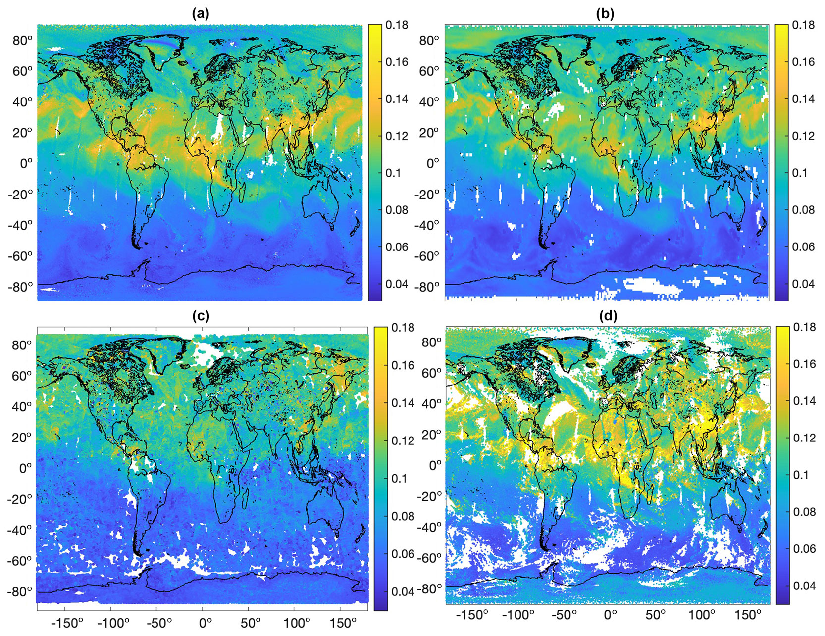
Figure 17 (a, b) Map plots of VMR (ppmv) of CO at 500 hPa from SNPP CrIS SiFSAP and SNPP CrIS CLIMCAPS for 12 May 2020, respectively; (c) the corresponding MOPITT CO VMR at 500 hPa (during 10–14 May 2020, to ensure a global-scale spatial coverage); (d) Metop-B IASI FORLI CO VMR at 500 hPa.

Figure 18 compares the total column of O₃ on 19 September 2019 from SNPP CrIS SiFSAP with that from SNPP CrIS CLIMCAPS, SNPP OMPS (Ozone Mapping and Profiling Suite; Jaross, 2017), and the Metop-B FORLI daily O₃ product. The ozone hole over the Antarctica region is clearly captured by all products. It is noted here that IR sensors like CrIS, AIRS, and IASI are generally more sensitive to the ozone distribution in the upper troposphere, while ultraviolet measurements like OMPS are more sensitive to stratospheric ozone. Both instruments can measure the tropospheric columns but lack vertical sensitivity in the troposphere (Fu et al., 2018). The results from two products (SiFSAP and CLIMCAPS) using the same sounder measurements agree well over most of the area.

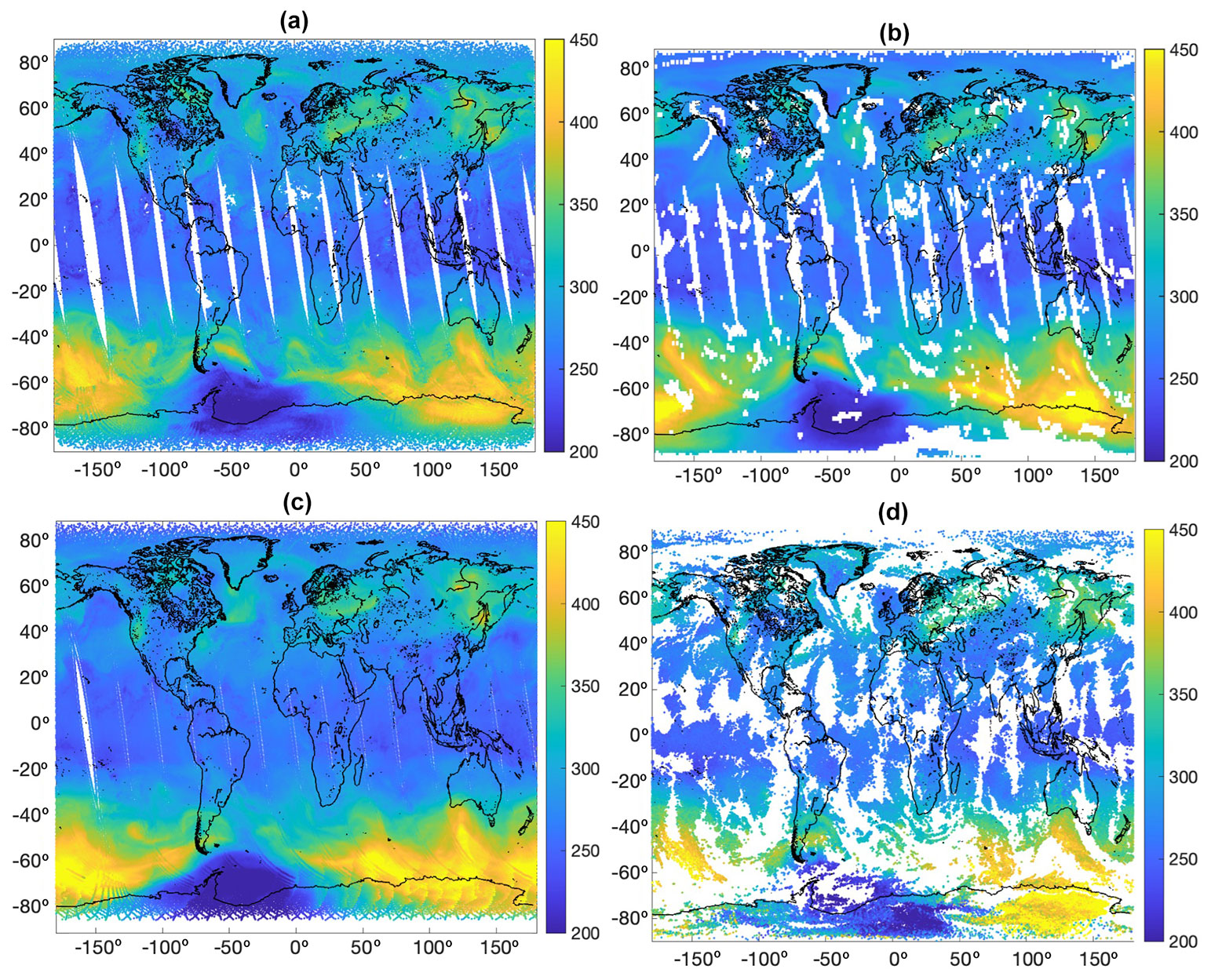
Figure 18 O₃ total column amount (DU, Dobson unit) retrieved from satellite-based observations on 20 September 2019 (a: SNPP CrIS SiFSAP; b: SNPP CrIS CLIMCAPS; c: SNPP OMPS; d: Metop-B IASI FORLI).

Figures 17 and 18 show that the SiFSAP system works effectively under all-sky conditions. As compared with FORLI, which only provides CO and O₃ data for cloud-free or almost-clear (with a cloud fraction less than 13 %) observations (George et al., 2009; Boynard et al., 2018), the capability of accounting for the cloud scattering in the SiFSAP algorithm ensures a much higher retrieval yield rate. Although CLIMCAPS can retrieve CO for most of the observations under cloudy-sky conditions, it fails in the area under overcast skies (shown as white area in Figs. 17 and 18) because the lack of contrast between observations of adjacent FOVs imposes challenges on the implementation of the cloud-clearing method.

Validation to CO₂, N₂O, and CH₄ from SiFSAP is very limited and remains to be completed in the near future. Therefore, these products are still subject to more research and improvement.

4.5 Cloud properties

Cloud optical depth, particle size, and cloud height (represented by the cloud top temperature, CTT) are simultaneously retrieved along with other geophysical variables in the SiFSAP algorithm. Details about the cloud-scattering model can be found in previously published PCRTM and physical-retrieval algorithm papers (Liu et al., 2006, 2007, 2009; Wu et al., 2017). Cloud properties for one individual CrIS footprint are retrieved under the assumption of one effective single layer with the cloud transmittance, reflectance, and emissivity defined by the optical depth and the particle size. Ice and water clouds are discerned based on the overall spectral characteristics of the cloud emissivity (transmittance). In the iterative retrieval process, both cloud phase options are tried and the one providing the best spectral fitting is saved as the solution. Earlier simulation studies have shown that the cloud phase can be retrieved with a very high accuracy rate (>95 %) if the hyper-spectral feature of the ice and water clouds can be fully explored (Wu et al., 2017).

Cloud properties from hyper-spectral sounder measurements can be validated using collocated imager observations like MODIS or VIIRS (Visible Infrared Imaging Radiometer Suite; e.g., Yue et al., 2022). The collocated SNPP CrIS and VIIRS cloud data (Fetzer et al., 2022) based on the VIIRS Atmosphere L2 Cloud Properties Product (Platnick et al., 2017; Heidinger and Li, 2017) are used to validate the cloud properties from SiFSAP for SNPP CrIS. Since VIIRS does not have IR channels in the 13 µm CO₂ absorption band, the MODIS CO₂ slicing solution for cloud top pressure retrievals for cold clouds is replaced with an IR window channel optimal-estimation approach coupled with CALIPSO-derived (Cloud-Aerosol Lidar and Infrared Pathfinder Satellite Observations) a priori constraints (Heidinger et al., 2019). The CTT of SiFSAP CrIS is compared with the average values of the CTT of VIIRS pixels within the CrIS footprints as shown in Fig. 19. The global-scale spatial distribution of CTT from SiFSAP agrees well with that from the VIIRS cloud product except in the Arctic region, where CTT retrieved from CrIS measurements tends to be warmer than VIIRS results. The correlation coefficient between the VIIRS CTT and CrIS CTT shown in Fig. 19 is larger than 0.93. Uncertainty in retrieved cloud properties tends to be larger for very thin clouds due to the challenge of extracting weak IR spectral signatures embedded in the measurement or forward-simulation errors. Figure 19 only shows results with retrieved cloud optical thicknesses larger than 0.4 (cloud emissivity larger than 0.1) to better illustrate the retrieval accuracy when there is adequate measurement-provided information. A correlation coefficient larger than 0.8 can still be achieved even when we include more thin cloud footprints with an optical depth as small as 0.05.

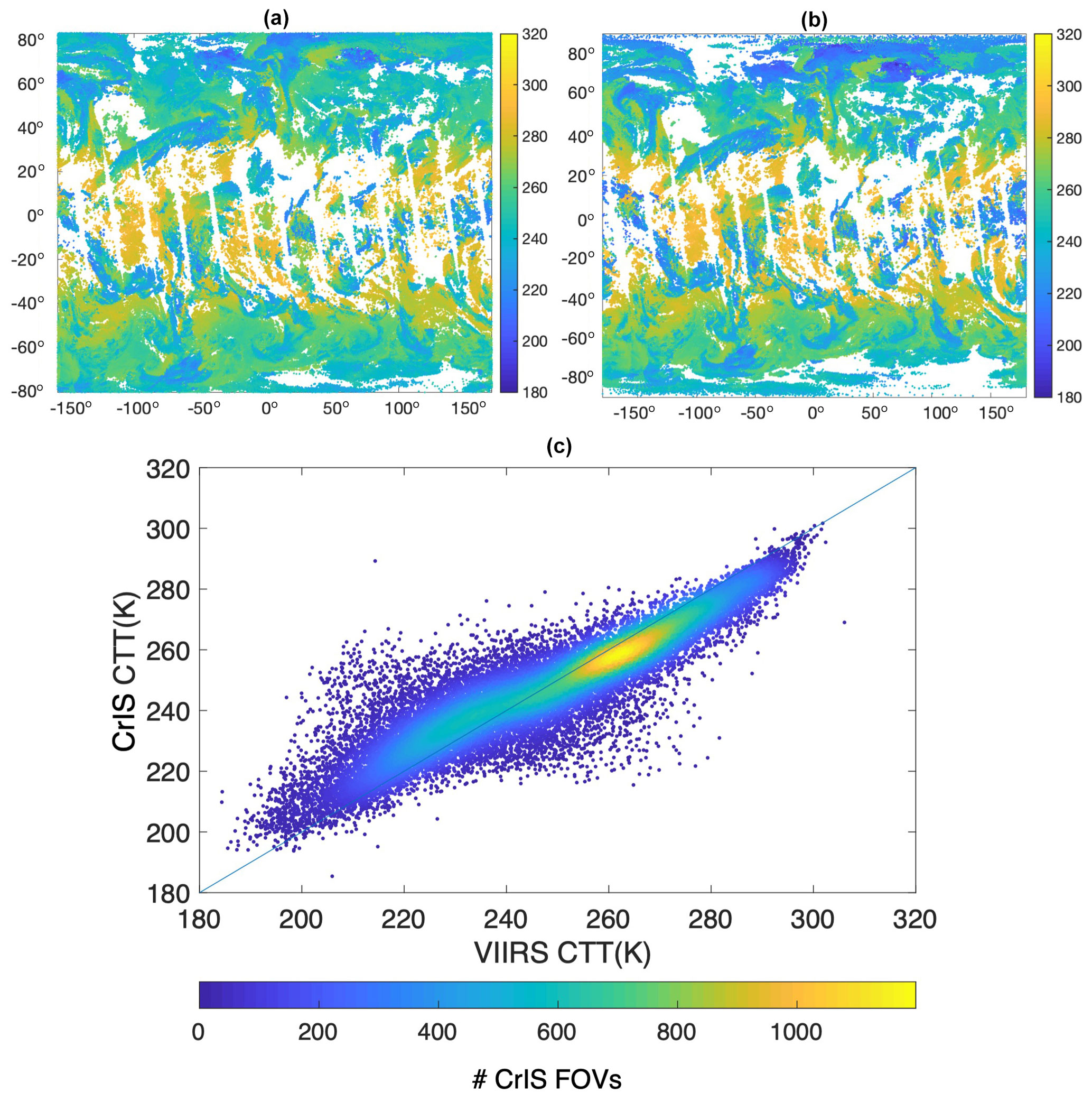
Figure 19 Cloud top temperature (K) for 1 January 2016 from (a) SNPP CrIS SiFSAP and (b) SNPP VIIRS cloud data products collocated to CrIS footprints; (c) the corresponding scatterplot.

Direct comparison between the effective cloud optical depth (COD) and the effective particle radius (R_e) retrieved for an individual CrIS FOV and the corresponding mean values for the collocated VIIRS pixels within the CrIS FOV can be challenging due to several factors. First, the spatial heterogeneity among VIIRS pixels means the IR radiative contribution from a cloud layer with an averaged VIIRS COD can be very different from the combined contribution from individual VIIRS pixels due to the nonlinear nature of the radiative transfer:

$$\begin{array}{}\text{(20)}& F\left(\stackrel{\mathrm{‾}}{\text{COD}},\stackrel{\mathrm{‾}}{R_{\mathrm{e}}}\right)\ne {\sum }_{i=\mathrm{1}}^N{\displaystyle \frac{F\left({\text{COD}}_i,R_{{\mathrm{e}}_i}\right)}{N}},\end{array}$$

where F is the forward operator. Second, the inconsistency between the cloud-scattering models used for sounder retrieval and for imager retrieval can further introduce large biases or uncertainties between two sets of COD and R_e. Third, inconsistency can also arise from a lack of consistency and accuracy in the atmospheric and surface state assumed for the cloud property retrievals. As compared with COD and R_e, it is relatively more straightforward to compare the effective cloud emissivity (fraction) values retrieved from CrIS and VIIRS measurements. The CrIS FOV cloud emissivity can be related to the VIIRS pixel effective cloud emissivity and the corresponding spatial fraction under the assumption that the total thermal emissions measured by CrIS and VIIRS within the same spectral band are consistent:

$$\begin{array}{}\text{(21)}& \begin{array}{rl}& B_{\mathit{\nu }}\left(T_{\mathrm{C}}^{\mathrm{CrIS}}\right){\mathit{ϵ}}_{\mathrm{C}}^{\mathrm{CrIS}}+B_{\mathit{\nu }}\left(T_{\mathrm{S}}\right){\mathit{ϵ}}_{\mathrm{S}}\left(\mathrm{1}-{\mathit{ϵ}}_{\mathrm{C}}^{\mathrm{CrIS}}\right)\\ & =f{\sum }_{i=\mathrm{1}}^N{\mathit{ϵ}}_{\mathrm{C},i}^{\mathrm{VIIRS}}{B}_{\mathit{\nu }}\left(T_{\mathrm{C},i}^{\mathrm{VIIRS}}\right)\\ & +\left(\mathrm{1}-f{\sum }_{i=\mathrm{1}}^N{\mathit{ϵ}}_{\mathrm{C},i}^{\mathrm{VIIRS}}\right)B_{\mathit{\nu }}\left(T_{\mathrm{S}}\right){\mathit{ϵ}}_{\mathrm{S}},\end{array}\end{array}$$

where B_ν represents the Planck function at wavenumber ν; ${\mathit{ϵ}}_{\mathrm{C}}^{\mathrm{CrIS}}$ and $T_{\mathrm{C}}^{\mathrm{CrIS}}$ are CrIS cloud emissivity and CTT; ${\mathit{ϵ}}_{\mathrm{C},i}^{\mathrm{VIIRS}}$ and $T_{\mathrm{C},i}^{\mathrm{VIIRS}}$ are the cloud emissivity and CTT of individual VIIRS pixels; f represents the spatial fraction of VIIRS cloud pixels within a CrIS FOV; and T_S and ϵ_S are surface skin temperature and surface emissivity, which are assumed to be homogeneous within a single CrIS FOV. Equation (21) is justified under the condition that ν is within a “window” spectral region where atmospheric absorption and thermal emission can be neglected, and the effective cloud reflectivity is close to 0. Therefore, the cloud transmissivity is approximated as 1−ϵ_C. A more simplified form can be used by utilizing the fact that the Planck function is linear enough and the surface emissivity is close to unity.

$$\begin{array}{}\text{(22)}& \begin{array}{rl}& {\mathit{ϵ}}_{\mathrm{C}}^{\mathrm{CrIS}}{T}_{\mathrm{C}}^{\mathrm{CrIS}}+\left(\mathrm{1}-{\mathit{ϵ}}_{\mathrm{C}}^{\mathrm{CrIS}}\right)T_{\mathrm{S}}={\sum }_{i=\mathrm{1}}^N{f}_i{\mathit{ϵ}}_{\mathrm{C},i}^{\mathrm{VIIRS}}{T}_{\mathrm{C},i}^{\mathrm{VIIRS}}\\ & +\left(\mathrm{1}-f{\sum }_{i=\mathrm{1}}^N{\mathit{ϵ}}_{\mathrm{C},i}^{\mathrm{VIIRS}}\right)T_{\mathrm{S}}\end{array}\end{array}$$

Such an approach to check the radiometric consistency between cloud properties from IR sounders and imagers has been used in the AIRS–MODIS cloud retrieval validation study (Kahn et al., 2007; Nasiri et al., 2011). Figure 20 demonstrates the comparison between the effective brightness temperature of CrIS $T_{\mathrm{eff}}^{\mathrm{CrIS}}$ and that of corresponding VIIRS measurements $T_{\mathrm{eff}}^{\mathrm{VIIRS}}$, with the definition being given as

$$\begin{array}{}\text{(23)}& {\displaystyle }{T}_{\mathrm{eff}}^{\mathrm{CrIS}}={\mathit{ϵ}}_{\mathrm{C}}^{\mathrm{CrIS}}{T}_{\mathrm{C}}^{\mathrm{CrIS}}+\left(\mathrm{1}-{\mathit{ϵ}}_{\mathrm{C}}^{\mathrm{CrIS}}\right)T_{\mathrm{S}},\text{(24)}& {\displaystyle }{T}_{\mathrm{eff}}^{\mathrm{VIIRS}}=f{\sum }_{i=\mathrm{1}}^N{\mathit{ϵ}}_{\mathrm{C},i}^{\mathrm{VIIRS}}{T}_{\mathrm{C},i}^{\mathrm{VIIRS}}+\left(\mathrm{1}-f{\sum }_{i=\mathrm{1}}^N{\mathit{ϵ}}_{\mathrm{C},i}^{\mathrm{VIIRS}}\right)T_{\mathrm{S}}.\end{array}$$

A good agreement is found between $T_{\mathrm{eff}}^{\mathrm{CrIS}}$ and $T_{\mathrm{eff}}^{\mathrm{VIIRS}}$, except for a small percentage of samples in the Arctic. The cloud emissivity data used for this study are the retrieval results based on NOAA Daytime Cloud Optical and Microphysical Properties (DCOMP; Walther and Heidinger, 2012) algorithm. Li et al. (2020) found that VIIRS cloud data products tend to have larger uncertainties in polar regions due to the lack of VIIRS spectral measurements in IR water and CO₂ absorption channels. They found a major improvement for the cloud mask can be achieved over polar regions by fusing the collocated CrIS measurements in the missing spectral region with the VIIRS data. Although the radiative consistency between cloud properties from SiFSAP CrIS and those from VIIRS is high, the surface skin temperature T_S, CTT, and the cloud effective emissivity (fraction) are highly correlated with each other. Uncertainties in either T_S or CTT will introduce inconsistency between the effective emissivity from these two measurements. Even though the three parameters compensate each other in order to fit radiometrically into the observations, the effective cloud emissivity from CrIS and VIIRS measurements can still be quite different. This is especially the case when there is a lack of thermal contract between T_S and CTT.

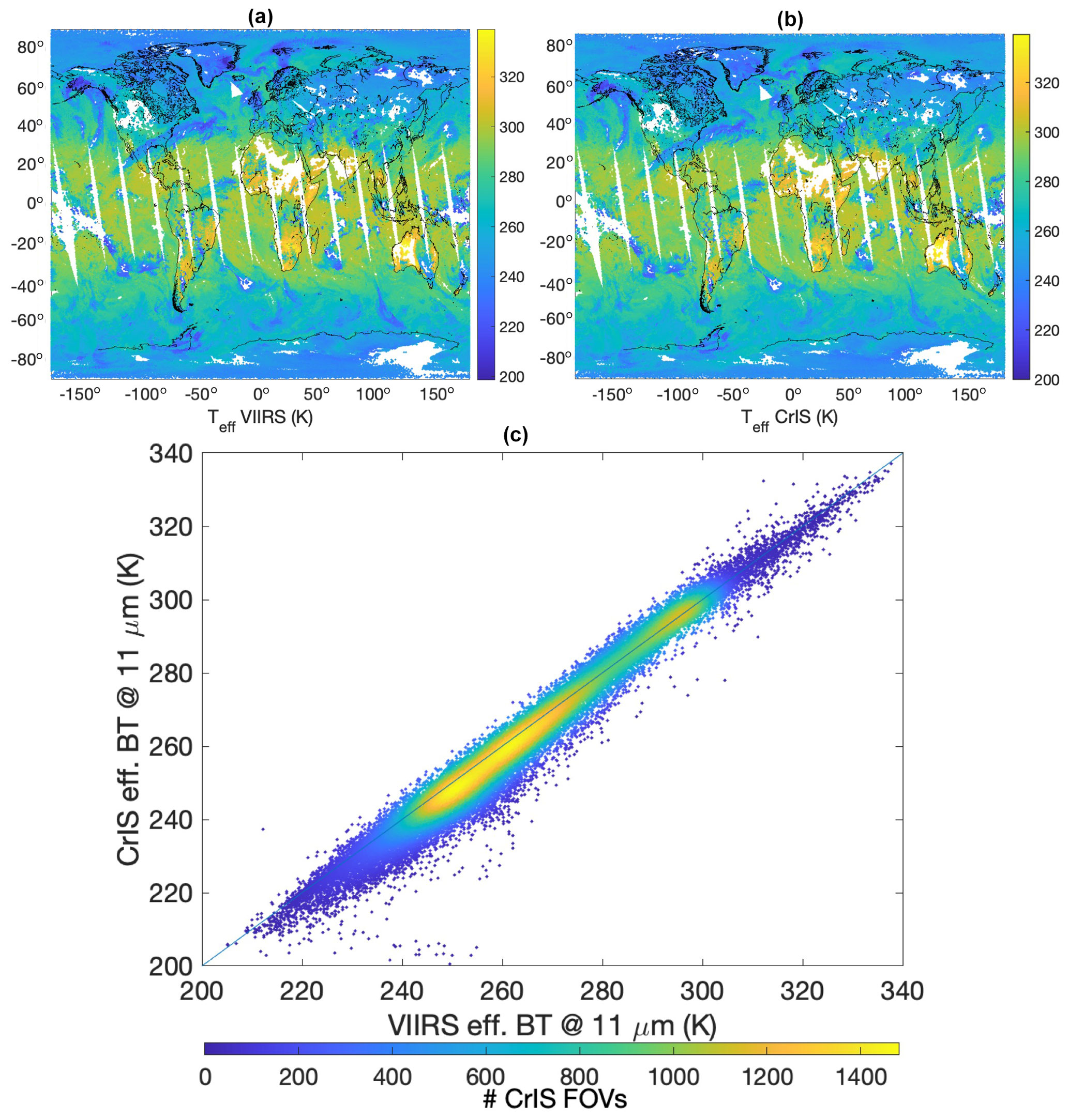
Figure 20 Effective brightness temperature (K) for 1 January 2016 from (a) SNPP CrIS SiFSAP and (b) SNPP VIIRS cloud data products collocated to CrIS footprints; (c) the corresponding scatterplot.

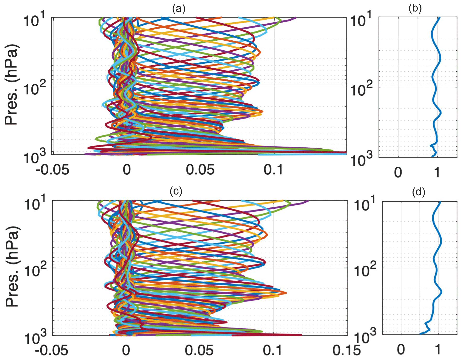
Figure 21 Sample temperature averaging kernels from SNPP CrIS SiFSAP: (a) averaging kernel under a clear-sky condition and (b) sum of averaging kernel rows at different pressure levels. Panels (c) and (d) represent those under a cloudy-sky condition.

Figure 22 Similar to Fig. 21 but for water vapor retrievals.

4.6 Averaging kernels

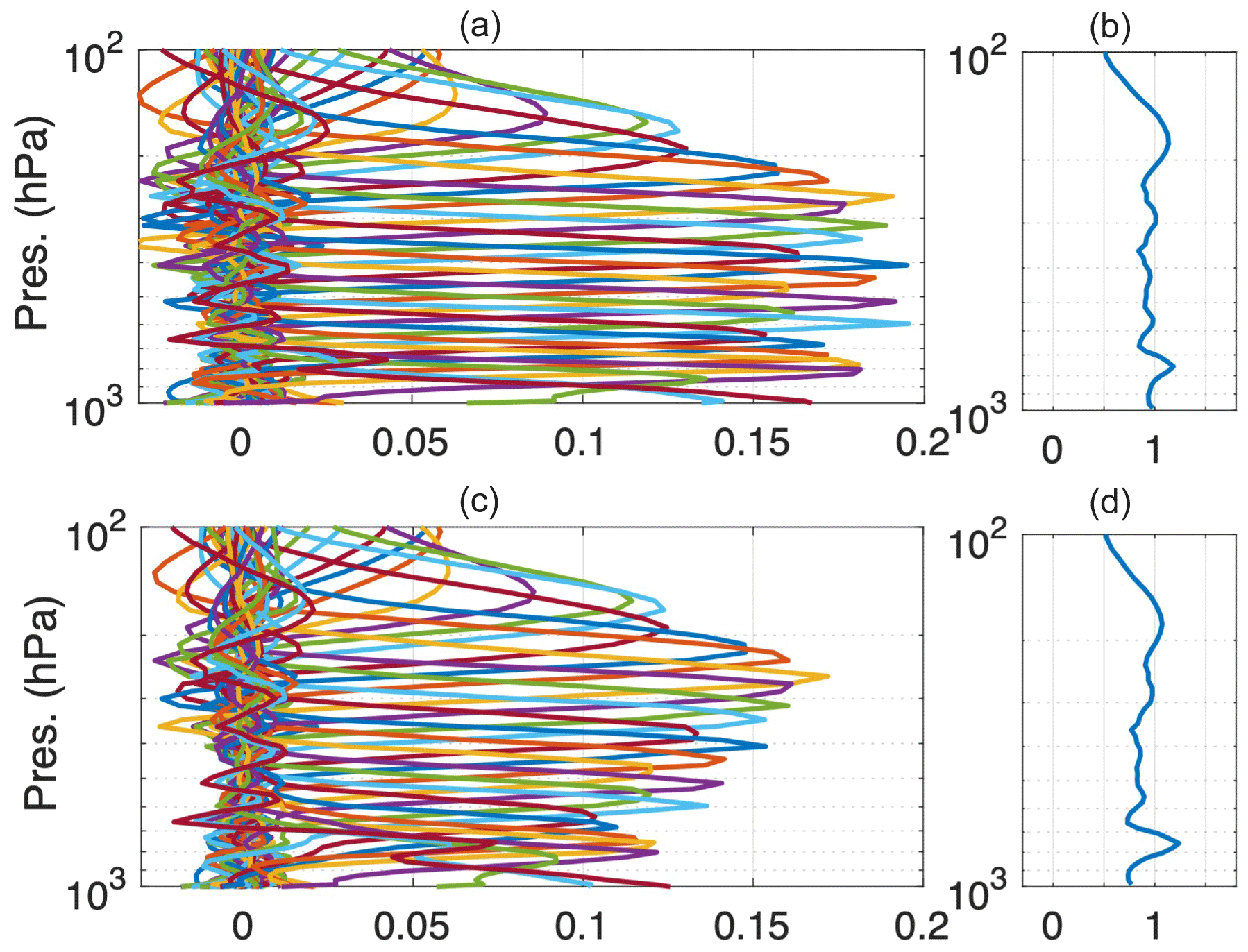
Hyper-spectral sounder measurements provide rich information for temperature and humidity vertical profiling. Figures 21 and 22 demonstrate typical temperature and water vapor retrieval averaging kernels from SNPP CrIS SiFSAP. Figure 21 clearly shows that high-vertical-resolution temperature retrieval can be achieved by the SiFSAP algorithm even in the lower-tropospheric region near the surface. The sum of the averaging kernel rows, also known as “verticality”, is usually used to characterize how much information comes from the measurements. A verticality value close to 1 means measurement provides dominant information so that a retrieval system's dependence on the a priori constraint is minimized. On the other hand, a verticality value close to 0 indicates that the system is heavily dependent on the a priori constraint since the measurement does not provide much information. Figure 21 shows that hyper-spectral measurements can resolve the temperature profile from the troposphere to the stratosphere under a clear-sky condition well. The information from the measurements degrades in the lower troposphere under a cloudy-sky condition region due to the weakening of the thermal-emission signal by clouds. The averaging kernel for water vapor retrieval (Fig. 22) is relatively less sensitive to clouds, but the information provided by hyper-spectral measurements to retrieve water vapor in the upper-troposphere and stratosphere region is limited.

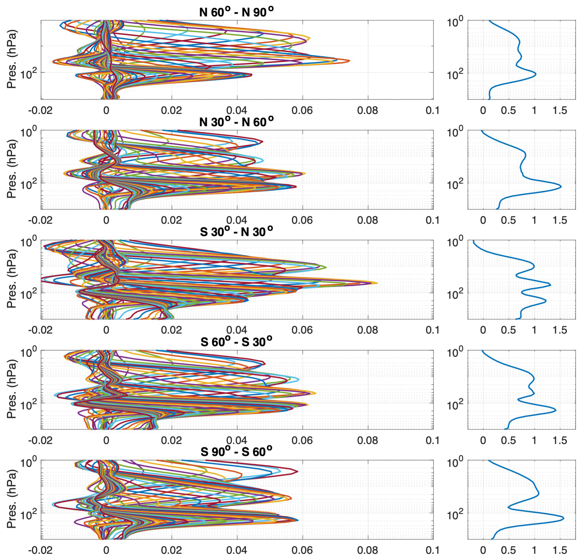
Figure 23 Ozone averaging kernels for 20 September 2019 from the SiFSAP algorithm for SNPP CrIS for different latitudinal regions.

As compared with temperature and water vapor, the measurement information from hyper-spectral IR sounders for trace gases retrieval is relatively limited and more scene dependent. Figure 23 shows the averaging kernels of the SNPP CrIS SiFSAP O₃ retrievals for 20 September 2019 for different latitudinal regions. The O₃ retrieval has sensitivity peaks in both the stratosphere and upper troposphere. The measurement sensitivity for lower-tropospheric O₃ is the highest in the tropical region and tends to decrease as the observations move to higher-latitude regions. Overall, the SiFSAP system provides a decent vertical resolution of O₃ profiling based on real CrIS observation data, which is comparable to what has been demonstrated for IASI measurements via an end-to-end simulation study (Wu et al., 2017).

Sample averaging kernels from the SiFSAP CO product are shown in Fig. 24 for different latitudinal bands, as CO retrieval is more latitudinally dependent than O₃. CrIS full-spectral-resolution measurements provide abundant information on the tropospheric CO retrieval in the tropical region (with verticality close to 1). The measurement information becomes less dominant in the mid-latitude region and very limited in the polar regions. This is partly due to the fact that thermal-emission signals due to CO absorption in the atmosphere are weaker in lower-temperature region. Ultimately, the total measurement sensitivity of CO is limited by the CrIS instrument noise level in the CO absorption spectral region. The vertical resolution of CO retrieval is very limited in the current version of SiFSAP. Similar to SiFSAP, the reported vertical resolution of CO retrieval in other IR sounder retrieval systems, e.g., FORLI, AIRS CO retrieval, and CLIMCAPS (George et al., 2009; Smith and Barnet, 2020), is also very limited. This can be ascribed to the weak thermal contrast among signals in CO measurement channels of IR sounders and the vertical-distribution constraints from the a priori constraints that remain to be optimized.

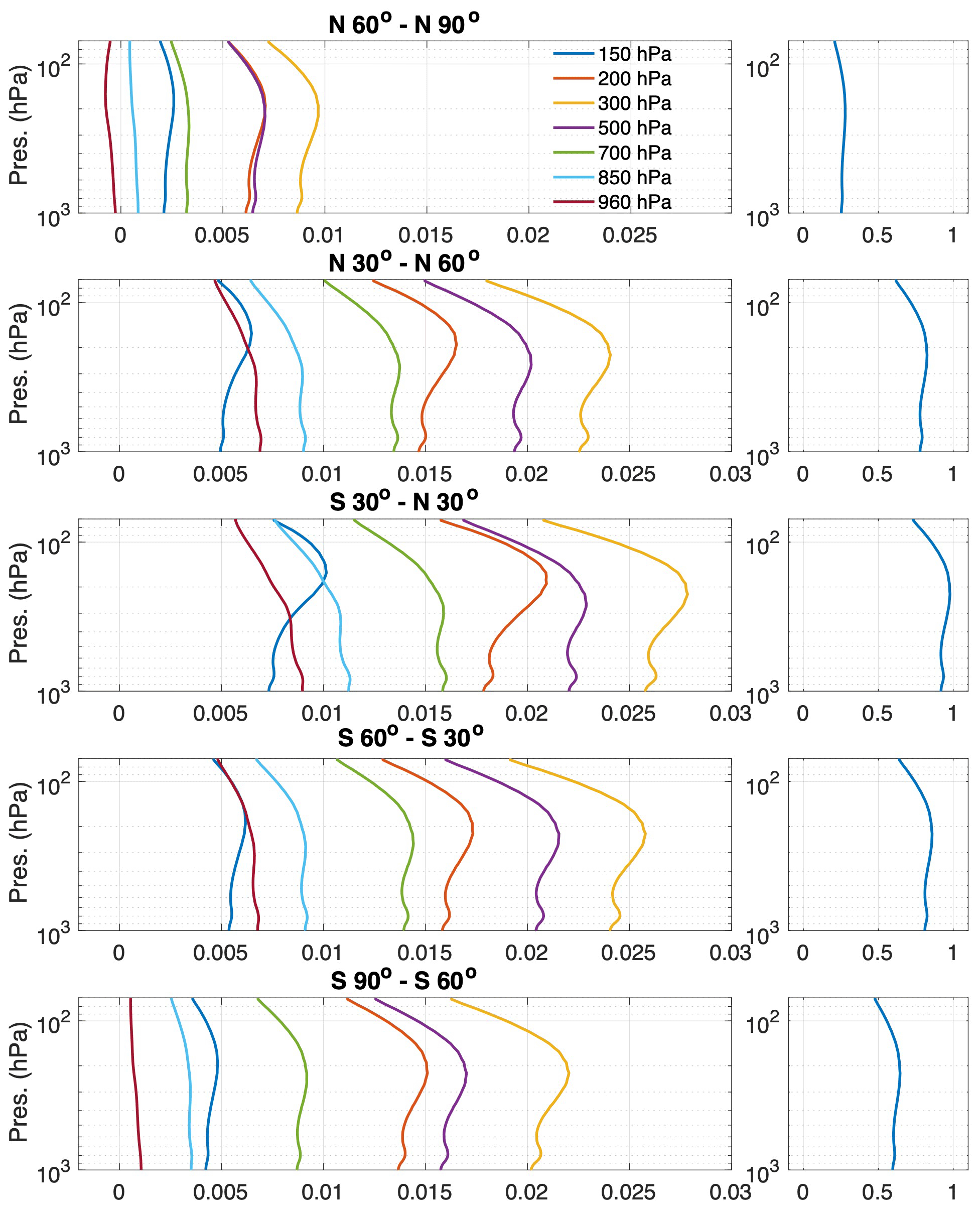
Figure 24 CO averaging kernels for 12 May 2020 from the SiFSAP algorithm for SNPP CrIS for different latitudinal regions.

5 Conclusions and future work

The SiFSAP retrieval algorithm has been developed to generate a high-spatial-resolution and radiometrically consistent hyper-spectral sounder product to explore the applications of sounder observations in areas that have not been fully addressed by the current operational sounder products. SiFSAP products include temperature, water vapor, O₃, CO₂, CO, CH₄, and N₂O profiles, as well as surface properties (including surface skin temperature and surface emissivity) and cloud properties (including cloud top pressure, height, temperature, effective cloud optical depth, and effective cloud particle size). Following an optimal-estimation scheme and the efficient and accurate forward radiative transfer model PCRTM, SiFSAP also provides users with the averaging kernels and error estimates to facilitate better uncertainty quantification in physical process studies and data assimilations using sounder products, as well as intercomparisons of multiple observational and model products.

Initial validation of key SiFSAP Level-2 variables has been carried out using SNPP CrIS as an example. More extensive studies and validation of SiFSAP products for other satellites will be conducted. Validation for CO₂, CH₄, and N₂O has been initiated, but a lot of work remains to be done, so these three trace gas products are released as exploratory data products at the current stage.

One key advantage of the SiFSAP algorithm is its applicability for multiple IR and MW sounder systems. In addition to CrIS and ATMS on board the SNPP and Joint Polar Satellite System (JPSS) satellites, the SiFSAP system is ready for the processing of both AIRS–AMSU and IASI–AMSU–MHS data. Simulation-based end-to-end studies and some evaluation work using sample IASI data have been demonstrated (Wu et al., 2017; Liu et al., 2009). Some AIRS retrieval case studies using the SiFSAP algorithm have already demonstrated the advantage of SiFSAP over traditional AIRS Level-2 products in capturing the high-spatial-resolution feature of gravity wave signals in stratospheric temperature (Wu et al., 2019). SiFSAP provides a solution to retrieve key climate variables from different hyper-spectral sounder observations using a consistent physical algorithm. This is not only important for effectively fusing information from multiple instruments but also essential to constructing a long-term continuous climate data record from the program-of-record sounder observations. The capability of using a unified radiative transfer model (i.e., PCRTM) to accurately fit the spectral radiances measured by all modern-era operational hyper-spectral sounders under all-sky conditions is essential for the climate trend/anomaly retrieval study from a radiometric consistency perspective.

SiFSAP will support weather and atmospheric dynamics studies by providing high-spatial-resolution temperature and water vapor profiles that can be used to reveal mesoscale atmospheric variations. The algorithm's capability of using the spectral information from all hyper-spectral channels via PC analysis makes it easy to be adapted and affordable for future sounder applications with a much higher spectral resolution and much more channels (e.g., IASI-NG). The scheme requires minimal auxiliary data to provide the a priori constraints and is suitable for real-time and environmental-monitoring applications. Future work includes exploring the SiFSAP algorithm's application potential in challenging areas (e.g., planetary boundary layer studies) by further improving the utilization of spectral information and the accommodation for forward-model errors. The development of a long-term climate record based on SiFSAP using the climate spectral-fingerprinting scheme is also underway.