Numerical model generation of test frames for pre-launch studies of EarthCARE's retrieval algorithms and data management system

The Earth Cloud, Aerosol and Radiation Explorer (EarthCARE) satellite consists of active and passive sensors whose observations will be acted on by an array of retrieval algorithms. EarthCARE's retrieval algorithms have undergone pre-launch verifications within a virtual observing system that consists of 3D atmosphere–surface data produced by the Global Environmental Multiscale (GEM) numerical weather prediction (NWP) model, as well as instrument simulators that when applied to NWP data yield synthetic observations for EarthCARE's four sensors. Retrieval algorithms operate on the synthetic observations, and their estimates go into radiative transfer models that produce top-of-atmosphere solar and thermal broadband radiative quantities, which are compared to synthetic broadband measurements, thus mimicking EarthCARE's radiative closure assessment. Three high-resolution test frames were simulated; each measures ∼6200 km along-track by 200 km across-track. Horizontal grid spacing is 250 m, and there are 57 atmospheric layers up to 10 mbar. The frames span wide ranges of conditions and extend over (i) Greenland to the Caribbean, crossing a cold front off Nova Scotia; (ii) Nunavut to Baja California, crossing over Colorado's Rocky Mountains; and (iii) the central equatorial Pacific Ocean, which includes a mesoscale convective system. This report discusses how the test frames were produced and presents their key geophysical features. All data are publicly available and, owing to their high-resolution, could be used to simulate observations for other measurement systems.

1 Introduction

The Earth Cloud, Aerosol and Radiation Explorer (EarthCARE) satellite mission, which is scheduled for launch in early to mid-2024, is a joint venture funded by the European Space Agency (ESA) and Japanese Aerospace Exploration Agency (JAXA) (Illingworth et al., 2015). The combination of Dopplerized cloud profiling radar (CPR), high-spectral-resolution lidar (ATLID), and multispectral imager (MSI) will facilitate synergistic retrievals of profiles of cloud, aerosol, and precipitation properties. Broadband top-of-atmosphere (TOA) radiances and fluxes calculated using these profiles will be compared to near-coincidental observations made by EarthCARE's broadband radiometer (BBR). This radiative closure assessment of retrievals will provide continuous feedback of performance to algorithm developers, as well as guidance to data users.

ESA's pre-launch phase of EarthCARE has relied much on the end-to-end simulation of measurements, retrievals, and data archiving procedures. The primary objective was to build a virtual observing system in which retrieval algorithms, developed expressly for EarthCARE, get applied to synthetic observations that resemble closely those that will be made by all of EarthCARE's sensors. The initial step of this multi-stage process is the definition of atmosphere–surface conditions. The obvious starting point was single homogeneous columns, but this quickly evolved into numerical simulation of realistic conditions for domains that span substantial portions of EarthCARE's planned orbit. These atmosphere–surface conditions are then operated on by instrument simulators that yield synthetic observations suitable for ingestion by retrieval algorithms. One could stop here and assess performance by comparing retrieved geophysical quantities to their simulated counterparts (see Mason et al., 2023), but in the real mission this is impossible to do routinely. As such, the next step in the end-to-end simulation chain is the application of radiative transfer models to retrieved geophysical properties. This produces radiometric quantities that are commensurate with synthetic BBR observations that are derived from the application of similar radiative transfer models directly to the simulated atmosphere–surface fields. The comparison of these quantities defines the radiative closure assessment of EarthCARE's retrievals.

EarthCARE's data-handling system processes observations into eight “frames” per orbit. As such, frames are ∼6500 km in the along-track direction. Their across-track width is 150 km as defined by the MSI's swath. Almost all measured and retrieved products are reported on the Joint Standard Grid (JSG), whose resolutions are ∼1 km in both horizontal directions and 0.5 km in the vertical. It was established early on, by EarthCARE's science and engineering teams, that synthetic observations for end-to-end experiments need to cover entire frames and be resolved horizontally to better than 1 km. Environment and Climate Change Canada's (ECCC) numerical weather prediction (NWP) model, known as the Global Environment Multiscale (GEM) model (Côté et al., 1998; Girard et al., 2014), was used to produce three such test frames with horizontal grid spacings of 250 m and 57 atmospheric layers up to 10 mbar. The frames include wide ranges of conditions and extend from (i) Greenland to the Caribbean, crossing a cold front off Nova Scotia; (ii) Nunavut to Baja California, crossing over Colorado's Rocky Mountains; and (iii) the central equatorial Pacific Ocean, including a mesoscale convective system. The primary purposes of this paper are to report on how these frames were constructed; their cloud, aerosol, and surface properties; and adjustments that were made to GEM's initial estimates of ice cloud particle sizes.

Full-frame datasets produced by GEM serve as input to the EarthCARE Simulator (ECSIM) (Voors et al., 2007). ECSIM consists of radiative transfer and instrument models that are coupled to databases of optical and microwave scattering properties. Bulk properties of atmospheric attenuators, such as 3D distributions of GEM's cloud water contents (CWCs), are used in conjunction with assumed aerosol and cloud size distributions in order for ECSIM to produce physically consistent synthetic measurements for each of EarthCARE's sensors. The production of simulated EarthCARE L1 data using ECSIM is described by Donovan et al. (2023). The use of high-resolution full-frame data in ECSIM not only allows assessment of the quality of EarthCARE's retrievals, but also facilitates the meaningful estimation of required computational resources and processing times for each algorithm.

The following section discusses how the test frames were defined. This is followed by descriptions of GEM and how it was configured and used for this study. Aerosols and surface optical properties were added to GEM's atmospheres, and these procedures are discussed in Sects. 4 and 5. Section 6 presents, and to a limited extent verifies, the simulated frames. Section 7 discusses issues with, and subsequent modifications to, GEM's simulated ice clouds. Concluding remarks and information regarding the acquisition of test frame data are provided in the final section.

2 Satellite orbit selection

Figure 1 shows several EarthCARE orbits, numbered 39316 through 39320. An orbit consists of eight frames, each frame's number having an appending letter from A to H, which is defined by given ranges of altitude (JAXA, 2017). Frames are color-coded and measure ∼5000 km along-track and 150 km across-track. All frames selected for testing correspond to local afternoon descending conditions (i.e., opposite to the A-Train). Assuming that nighttime atmospheric conditions are not fundamentally different from daytime conditions, night retrievals can be approximated by neglecting MSI solar channels and solar background for ATLID. Test frames should cover wide varieties of clouds, surfaces, and meteorological and solar illumination conditions. Locations and times needed to initialize simulations of test frames have been established by examining GOES satellite imagery and surface meteorological data. Also, A-Train's active sensor observations had to intersect the frame.

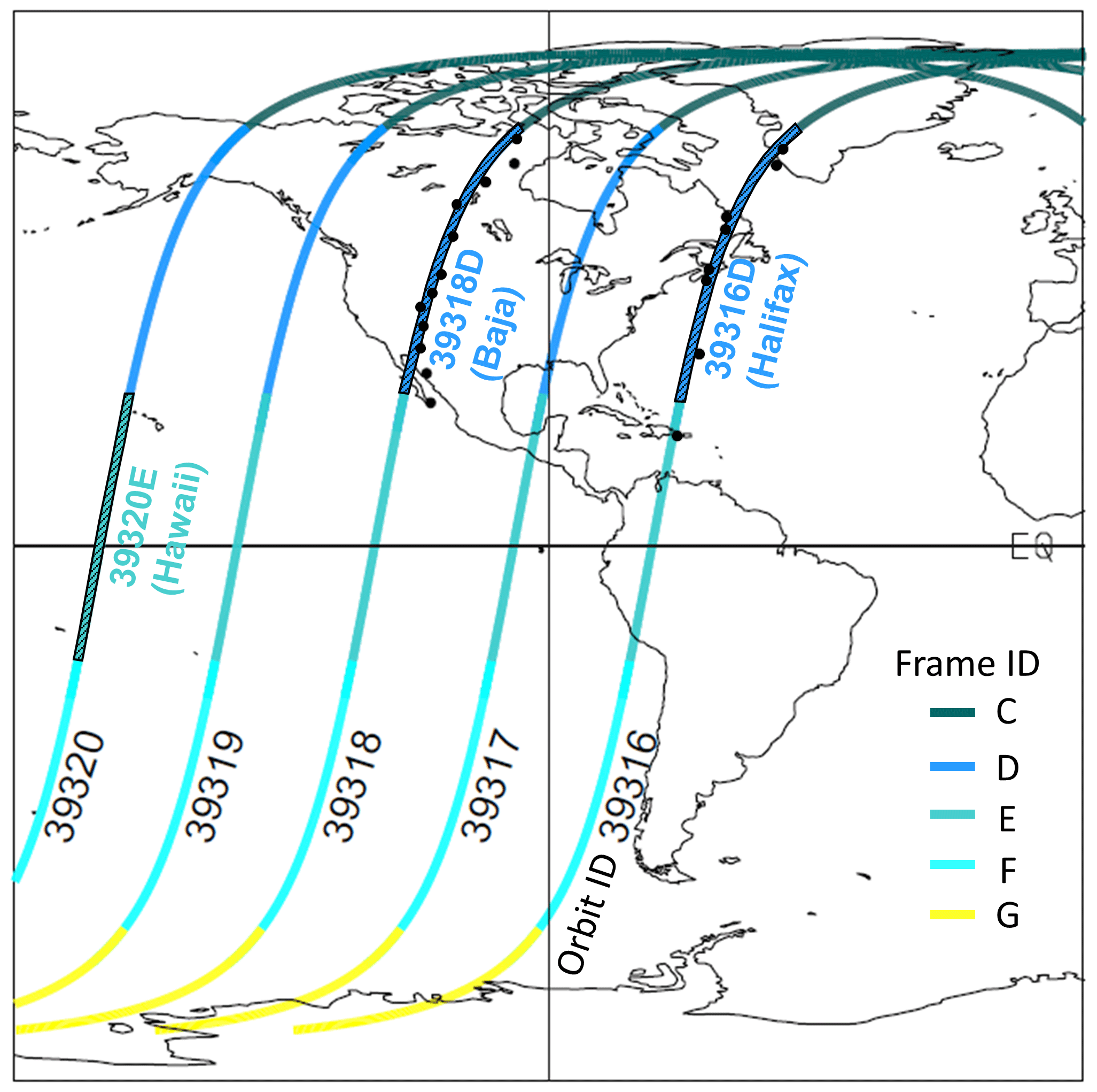
Figure 1 Examples of several successively numbered EarthCARE orbits as provided by ESA. Frames are color-coded with the test frames labeled as 39316D (Halifax), 39318D (Baja), and 39320E (Hawaii).

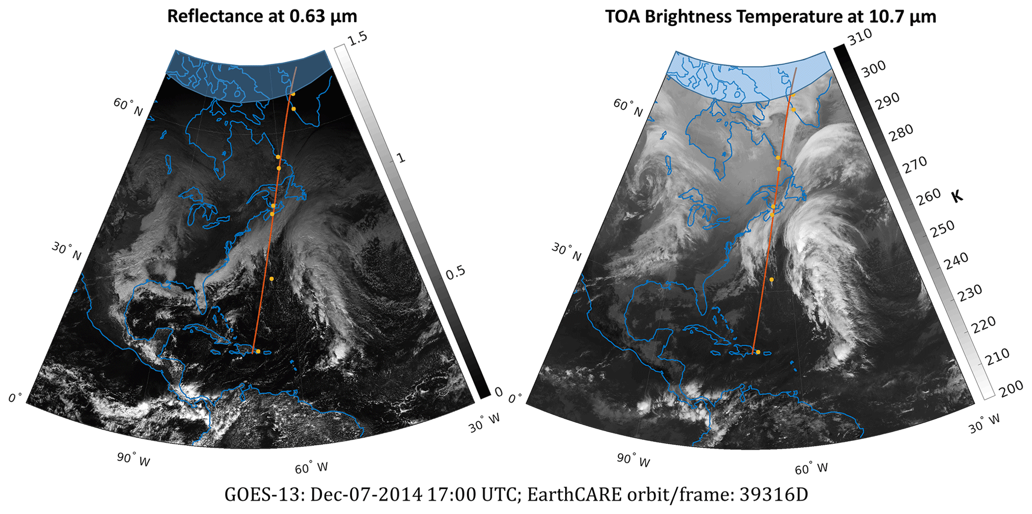
Figure 2 GOES-13 TOA reflectance at 0.63 µm and brightness temperature at 10.7 µm on 7 December 2014 at 18:00 UTC. Red lines indicate EarthCARE's track for the Halifax frame (see orbit 39316D in Fig. 1). Yellow dots mark locations of nearby surface meteorological stations. Blue shaded areas indicate GOES-13's northern limit of observation.

Table 1 Surface conditions (observed/modeled) near the Halifax frame (see orbit 39316D in Fig. 1) for 7 December 2014 at 18:00 UTC.

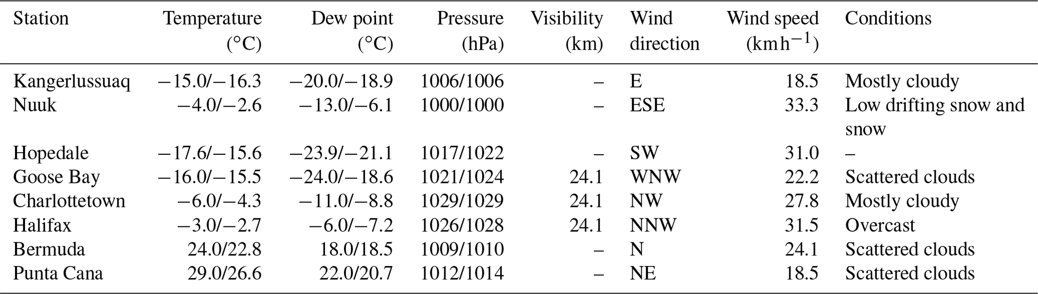
As Fig. 1 shows, frame 39316D extends from southern Greenland, across extreme eastern Canada, and to in the Atlantic Ocean roughly 500 km north of Dominican Republic. Because it passes close to the city of Halifax, Nova Scotia, it is referred to hereinafter as the “Halifax frame”. Figure 2 shows GOES-13 reflectances and TOA brightness temperatures for its 0.63 and 10.7 µm channels for 7 December 2014 at 18:00 UTC. Table 1 lists surface conditions reported at 18:00 UTC by several meteorological stations close to the ground track (see dots in both Figs. 1 and 2). This frame includes no sun over Greenland, cold surface air over eastern Canada, a cold front with deep clouds just off the coast of Nova Scotia, and scattered shallow clouds between Bermuda and Dominican Republic.

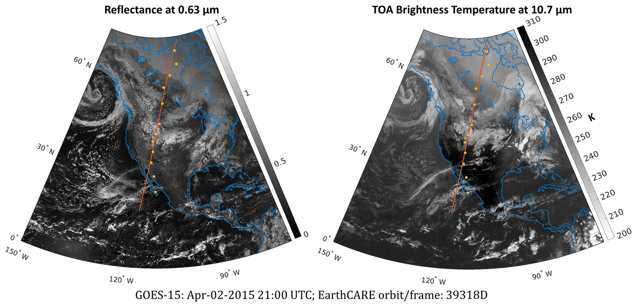
Figure 3 As in Fig. 1 but this is GOES-15 imagery for 2 April 2015 at 21:00 UTC. Red lines indicate the Baja frame (see orbit 39318D in Fig. 1).

Table 2 As in Table 1 but these are for the Baja frame (see orbit 39318D in Fig. 1) for 2 April 2015 at 21:00 UTC.

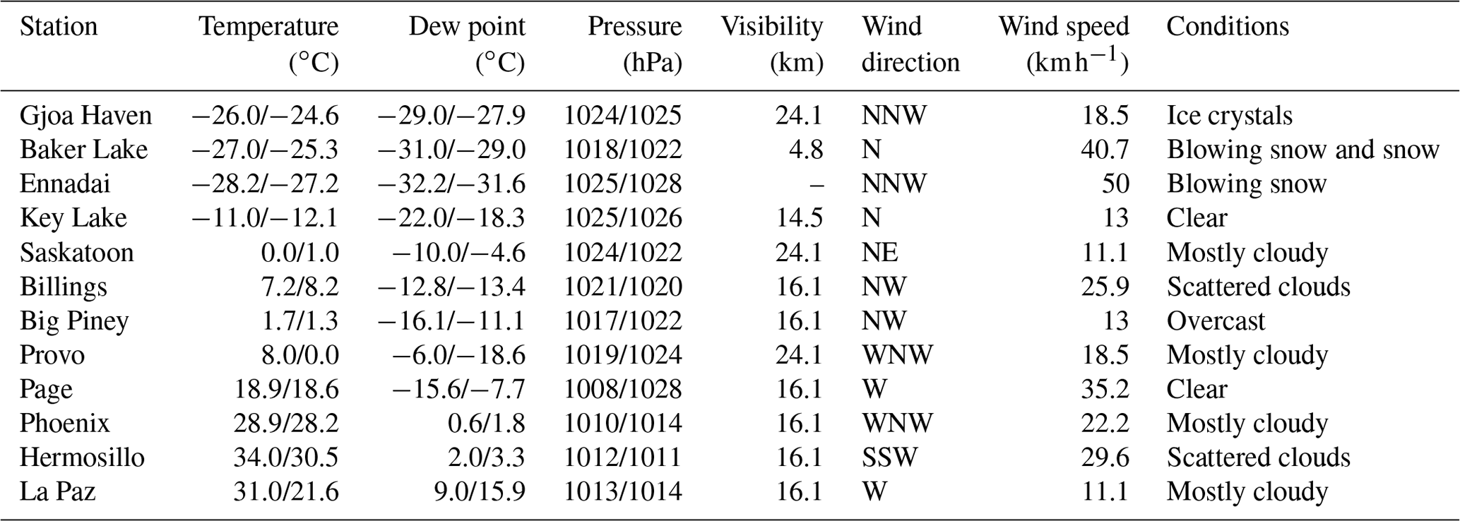
The second frame, 39318D, is referred to as the “Baja frame”. It stretches from the Canadian Arctic Archipelago, over central North America's Great Plains and Rocky Mountains, and to near Baja California Sur. Figure 3 shows GOES-15 imagery and EarthCARE's ground track for 2 April 2015 at 21:00 UTC. Table 2 lists surface conditions reported at 21:00 UTC. At the north end of this frame surface conditions were cold with blowing snow and largely cloudless. Through the Canadian Prairies there were low scattered clouds over snow-covered surfaces, while over the Rocky Mountains skies were very cloudy. In the southern reaches, skies were clear with some cirrus, and surface conditions were warm and very dry.

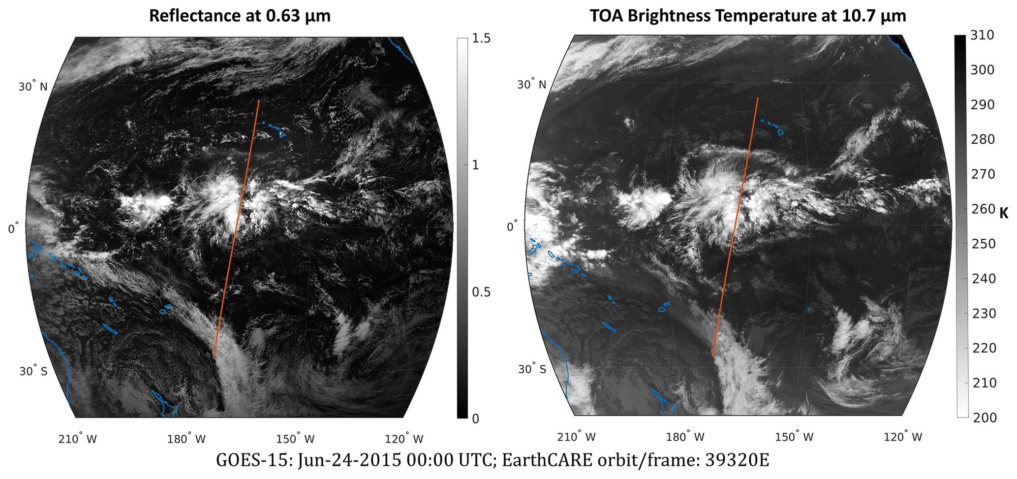
Figure 4 As in Fig. 1 but this is GOES-15 imagery for 24 June 2015 at 00:00 UTC. Red lines indicate the Hawaii frame (see orbit 39320E in Fig. 1).

The third frame, 39320E, as shown in Figs. 1 and 4, crosses the central Pacific Ocean, near Hawaii, on 24 June 2015. It is referred to as the “Hawaii frame”. GOES-15 imagery at 00:00 UTC on 24 June 2015 indicates that the central portion of the frame bisected a mesoscale convective system (MCS). North and south of the MCS, skies were mostly cloudless with some broken cloud at variable altitudes. There was also a weak frontal system at its southern extremity.

3 NWP model setup

The NWP model used to produce EarthCARE's test frames was ECCC's GEM model (Côté et al., 1998; Girard et al., 2014). GEM's dynamics are formulated in terms of the non-hydrostatic extension of the primitive equations with a terrain-following hybrid vertical grid. It can be run as a global model or a limited-area model and is capable of one-way self-nesting. For this work, GEM ran with four nested domains at horizontal grid spacings of Δx of 10, 2.5, 1, and 0.25 km, with 79 hybrid levels for the 10 km outer-domain and 57 for the other three. The global analysis data used in ECCC's Global Deterministic Prediction System (GDPS) (Buehner et al., 2015) were used as the initial condition for the outermost simulation domain at 10 km horizontal grid spacing. The GDPS predictions are also used as the lateral boundary conditions with the nesting method described in Thomas et al. (1998).

The simulations at Δx of 2.5, 1, and 0.25 km used Milbrandt and Yau's (2005a, b) double-moment bulk cloud microphysics scheme (referred to hereinafter as MY2), which predicts mass and number mixing ratio for each of six hydrometeor classes: non-precipitating liquid droplets, ice crystals, rain, snow, graupel, and hail. For the Δx=10 km domain, the Kain–Fritsch (KF) deep convection scheme (Kain and Fritsch, 1990, 1993) was used. Its liquid and ice CWCs are passed later to MY2 as non-precipitating liquid droplet and ice crystal categories.

In addition to MY2 and KF, a planetary boundary layer scheme can also produce liquid and ice clouds along with fractional cloudiness for cumulus and stratocumulus clouds (Bélair et al., 2005). Moreover, a shallow convection scheme (Bélair et al., 2005) also supplies estimates of liquid and ice CWCs and cloud fractions for cells with shallow cumulus. Both schemes are used in all domains.

The atmospheric turbulence is parameterized with a turbulent kinetic energy (TKE) scheme (Benoit et al., 1989; Bélair et al., 2005) named “MoisTKE”. For the simulations with 250 m horizontal grid spacing, a modified mixing length with an asymptotic value based on the horizontal grid size (${\mathit{\lambda }}_{\mathrm{0}}=\mathrm{0.23}(\mathrm{\Delta }x\mathrm{\Delta }y{)}^{\mathrm{1}/\mathrm{2}}$) is used. The readers are referred to Leroyer et al. (2014) for more details.

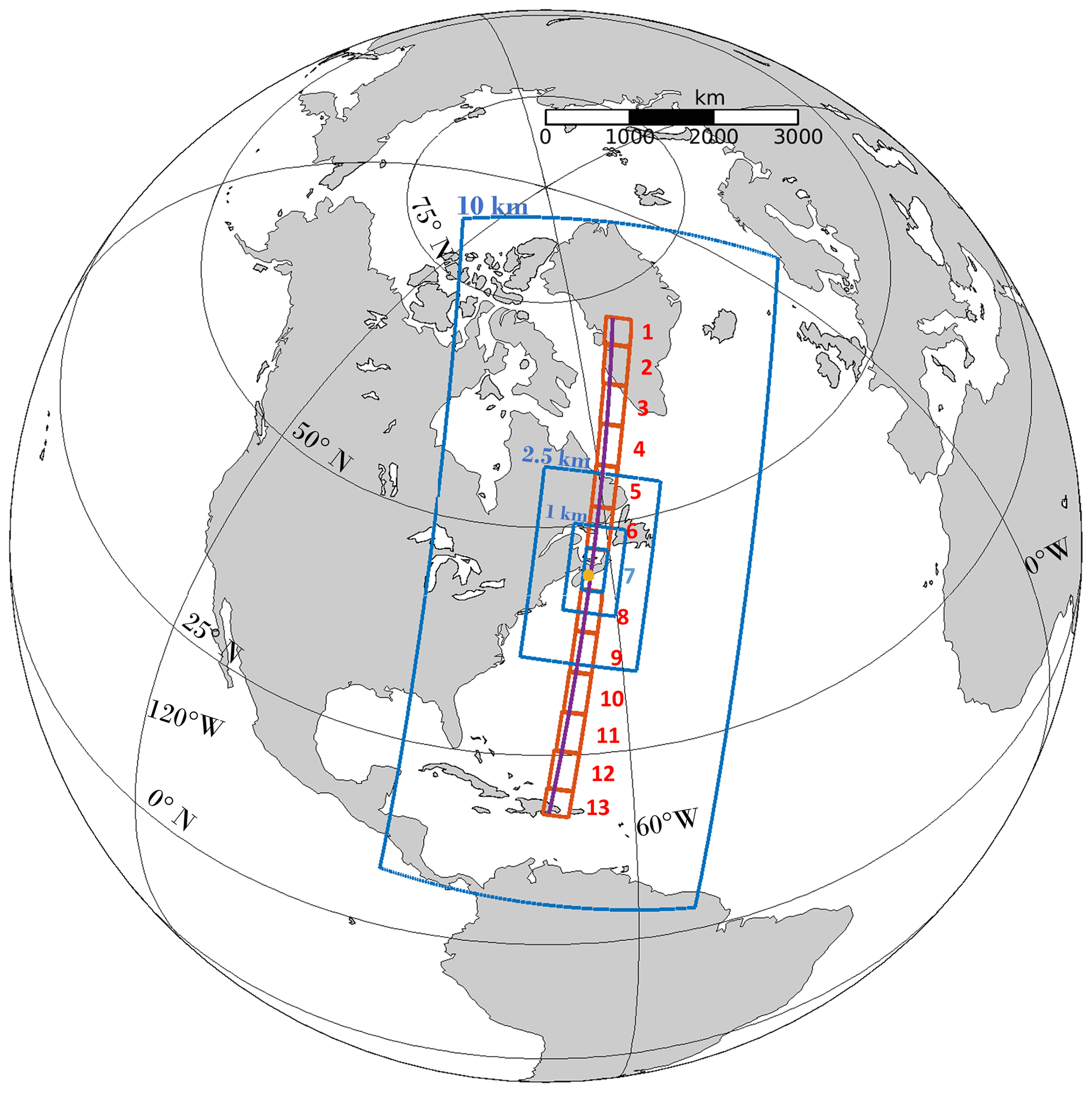
Figure 5 Downscaling domains for the Halifax frame (39316D). Blue rectangles delineate successive downscaling domains that culminate in the seventh innermost domain whose horizontal grid spacing is Δx=0.25 km. Red rectangles are the 12 other innermost domains for this frame. EarthCARE's ground track is indicated by the purple line, which is 60 km west of center.

Table 3 Sizes of GEM's downscaling domains (see Fig. 5) and their horizontal resolutions.

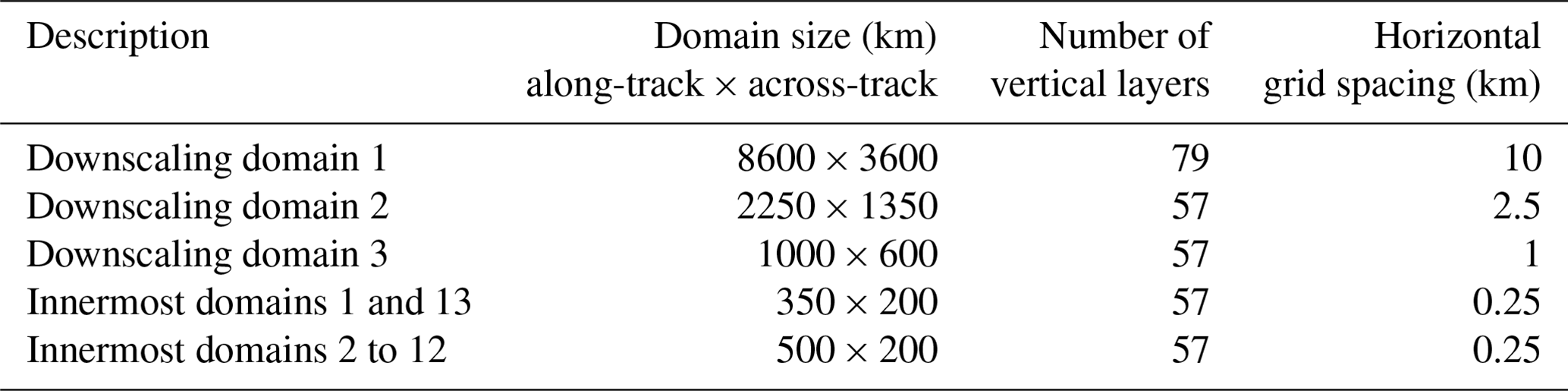
It was simplest to align GEM's “computational Equator” approximately along EarthCARE's orbit and divide 6200 km long frames into 13 non-overlapping inner-most domains (Δx=0.25 km) and run them separately: 11 segments at 500 km along-track and both end segments at 350 km (all are 200 km wide). The downscaling transitional domains at Δx of 2.5 and 1 km adapt themselves to the locations of the Δx=0.25 km domains (both domains at Δx of 2.5 and 1 km are repeated 13 times). A common Δx=10 km domain was used for all 13 segments. Figure 5 illustrates this configuration, and Table 3 summarizes domain sizes and Δx. Finally, the 13 inner-most domains are simply concatenated to form 6200 km frames. While this forms discontinuities, they are not a serious hindrance for the task at hand.

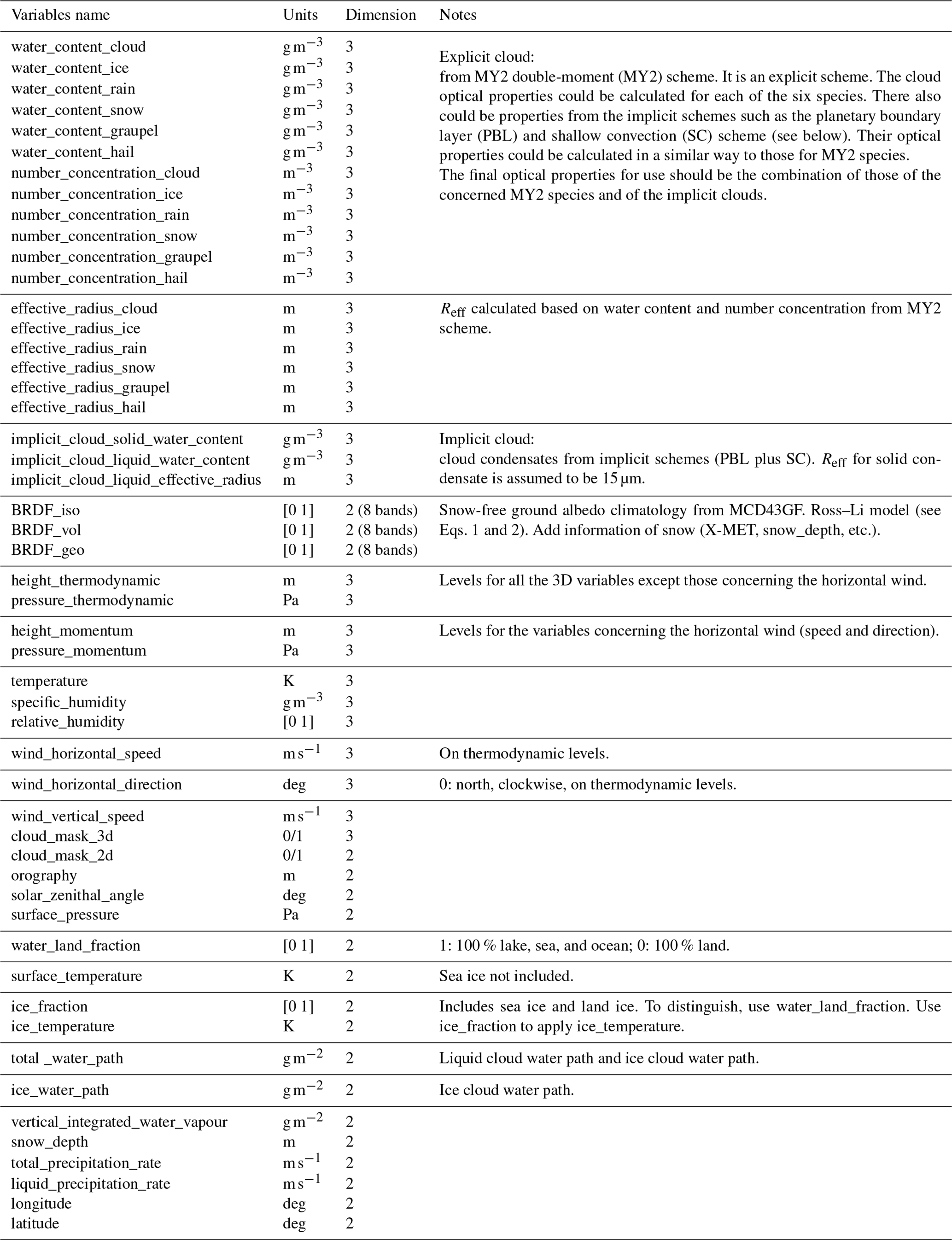
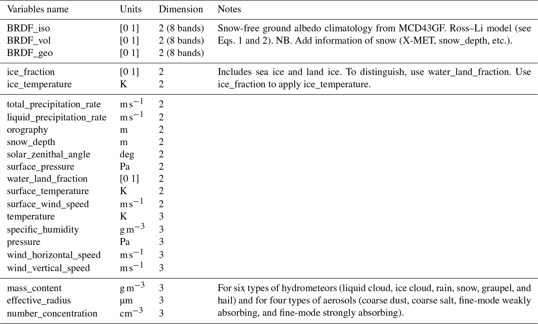
Simulations for the Halifax frame (39316D) were initialized at 12:00 UTC on 7 December 2014 and saved at 17:30 UTC. Likewise, the Baja frame (39318D) simulations were initialized at 12:00 UTC on 2 April 2015 and saved at 21:00 UTC, while the Hawaii frame was initialized at 12:00 UTC on 23 June 2015 and saved at 00:00 UTC on 24 June 2015. Data for all three frames are publicly available. Variables include CWC, number concentration, and effective radius R_eff for the six aforementioned hydrometeor types. Saved variables are listed in the Appendix.

4 Shortwave optical properties for land surfaces

As the additional data for pre-launch studies of EarthCARE, GEM's snow-free surface albedos were replaced by those based on MODIS's MCD43GF 1 km resolution bidirectional reflectance distribution function (BRDF) product for the period 2002 to 2013 (Schaaf et al., 2002). These data were interpolated, via nearest neighbor, to 0.25 km. Conditions for the Baja frame are shown here because it is primarily over land; the others are mostly over ocean.

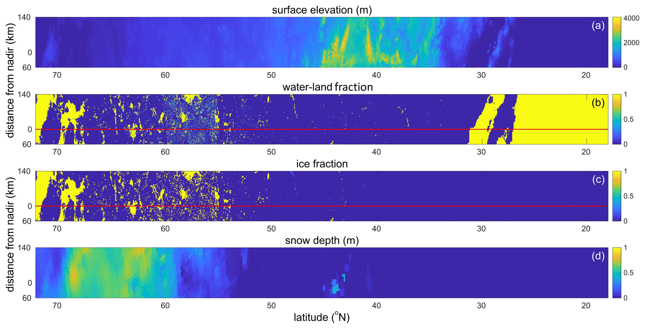
Figure 6 All panels are for the Baja frame (see Figs. 1 and 3) and each panel's title is self explanatory. For (b) and (c), blue (fraction of 0) corresponds to entirely land and yellow (fraction of 1) to either entirely water or entirely ice.

Figure 6a illustrates the wide range of surface conditions for the Baja frame. The Rocky Mountains are crossed near 40^∘ N, but this being mid-springtime only small amounts of mountain snow remain. Figure 6b highlights the distribution of freshwater lakes in the Canadian Shield; Fig. 6c shows that most are frozen and snow-covered. From Fig. 6c it is clear that shallow snow covers most of the Canadian Prairies with deeper snow north of the treeline, which for this frame is close to 60^∘ N (see 0.63 µm reflectances in Fig. 3).

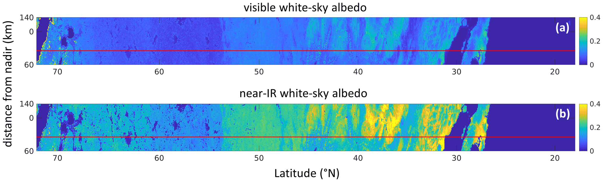
Figure 7 (a) Visible white-sky albedos, as defined in Eq. (2), for snow-free land for the Baja frame. (b) Same as (a) except these are near-IR values. EarthCARE's nadir track is shown by red lines.

Following Schaaf et al. (2002), spectral-dependent black-sky albedos are defined as

$$\begin{array}{}\text{(1)}& \begin{array}{rl}{\mathit{\alpha }}_{\text{bs}}& \left({\mathit{\theta }}_{\mathrm{0}}\right)=\\ & {\mathit{\alpha }}_{\mathrm{1}}+{\mathit{\alpha }}_{\mathrm{2}}(-\mathrm{0.007574}-\mathrm{0.070987}{\mathit{\theta }}_{\mathrm{0}}^{\mathrm{2}}+\mathrm{0.307588}{\mathit{\theta }}_{\mathrm{0}}^{\mathrm{3}})\\ & +{\mathit{\alpha }}_{\mathrm{3}}(-\mathrm{1.284909}-\mathrm{0.166314}{\mathit{\theta }}_{\mathrm{0}}^{\mathrm{2}}+\mathrm{0.041840}{\mathit{\theta }}_{\mathrm{0}}^{\mathrm{3}}),\end{array}\end{array}$$

where θ₀ is solar zenith angle in radians, and α₁, α₂, and α₃ are separate sets of spectral-dependent BRDF kernel weights for spectral ranges of 300–700 nm and 700–50 000 nm. Corresponding white-sky albedos are defined as

$$\begin{array}{}\text{(2)}& {\mathit{\alpha }}_{\text{ws}}={\mathit{\alpha }}_{\mathrm{1}}+\mathrm{0.189184}{\mathit{\alpha }}_{\mathrm{2}}-\mathrm{1.377622}{\mathit{\alpha }}_{\mathrm{3}}.\end{array}$$

Figure 7 shows α_ws for the Baja frame. Note that because these are snow-free values, they tend to be largest in the southern areas, especially in the near-IR for forests of western Colorado and deserts of Arizona and Sonora. With both variable surface elevation and surface albedos, this frame represents a stringent test for retrieval algorithms, as opposed to the more straightforward ocean surfaces that dominate the other two frames.

For snow- or ice-covered areas, snow depth or ice fraction and/or surface land type should be used to determine albedo. For ocean and lakes, wind speed is used to determine surface albedo. To determine surface emissivity for different types of surface, Huang et al.'s (2016) surface emissivity climatology was used. Surface albedo and emissivity are discussed further in another paper on broadband radiative quantities (ACM-COM and ACM-RT products) in this special issue (Cole et al., 2023).

5 Aerosol properties

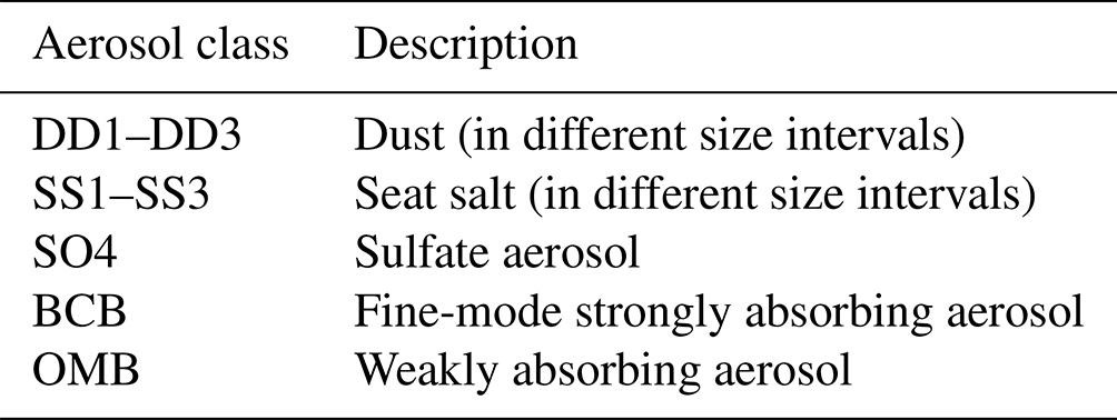
The ECSIM scene creation process requires 3D distributions of aerosol size distributions. As GEM lacks interactive aerosol tracers and chemistry, aerosol fields were added to the test scenes using information from the Copernicus Atmosphere Monitoring Service (CAMS) (Flemming et al., 2017). The CAMS data were at a resolution of 0.5^∘ by 0.5^∘ latitude–longitude and 60 hybrid sigma model levels. The aerosol scheme implemented within ECSIM follows the Hybrid End-To-End Aerosol Classification (HETEAC) approach of defining a certain set of basic aerosol types with associated, e.g., size distributions, refractive indices, and optical properties that, when weighted and summed, yield adequate representations of a wide range of observed aerosol optical properties (Wandinger et al., 2016, 2023). Table 4 lists the CAMS aerosol fields, and the Supplement provides a detailed description of the mapping between CAMS fields and ECSIM and HETEAC scattering types. It also provides more details regarding aerosol representation.

Table 4 Aerosol classes from the Copernicus Atmosphere Monitoring Service (CAMS).

6 Results: GEM simulations and verification

The purpose of this section is to show selected results that characterize the EarthCARE test frames produced directly by GEM. Post-simulation adjustments were made to ice microphysical properties as described and shown in both Sect. 7 and the Supplement.

6.1 Halifax frame

Figure 8a and c show MODIS spectral fluxes (MYD02HKM product; MCST, 2017) for 0.459–0.479 µm and 10.8–11.3 µm for the Halifax frame. Key cloud-related features are a cold front between 40 and 45^∘ N, scattered clouds to its south, and mostly overcast conditions to its north. Figure 8b and d show TOA spectral fluxes for two wavebands, close to MODIS's bands, as simulated by the Rapid Radiative Transfer Model for General Circulation Models (RRTMG; Mlawer et al., 1997; Iacono et al., 2000, 2008) using GEM data. At large scales, GEM did well with respect to cloud occurrence. Figure 8e and f show distributions of visible and infrared spectral fluxes, respectively. While the distributions of fluxes derived from observations and models follow similar patterns, there are some notable differences in the imagery. For the GEM scenes, discontinuities, stemming from the stitching together of the semi-independent high-resolution inner-most domains, are clearly visible across the frontal system. They do not pose a serious problem for the task at hand.

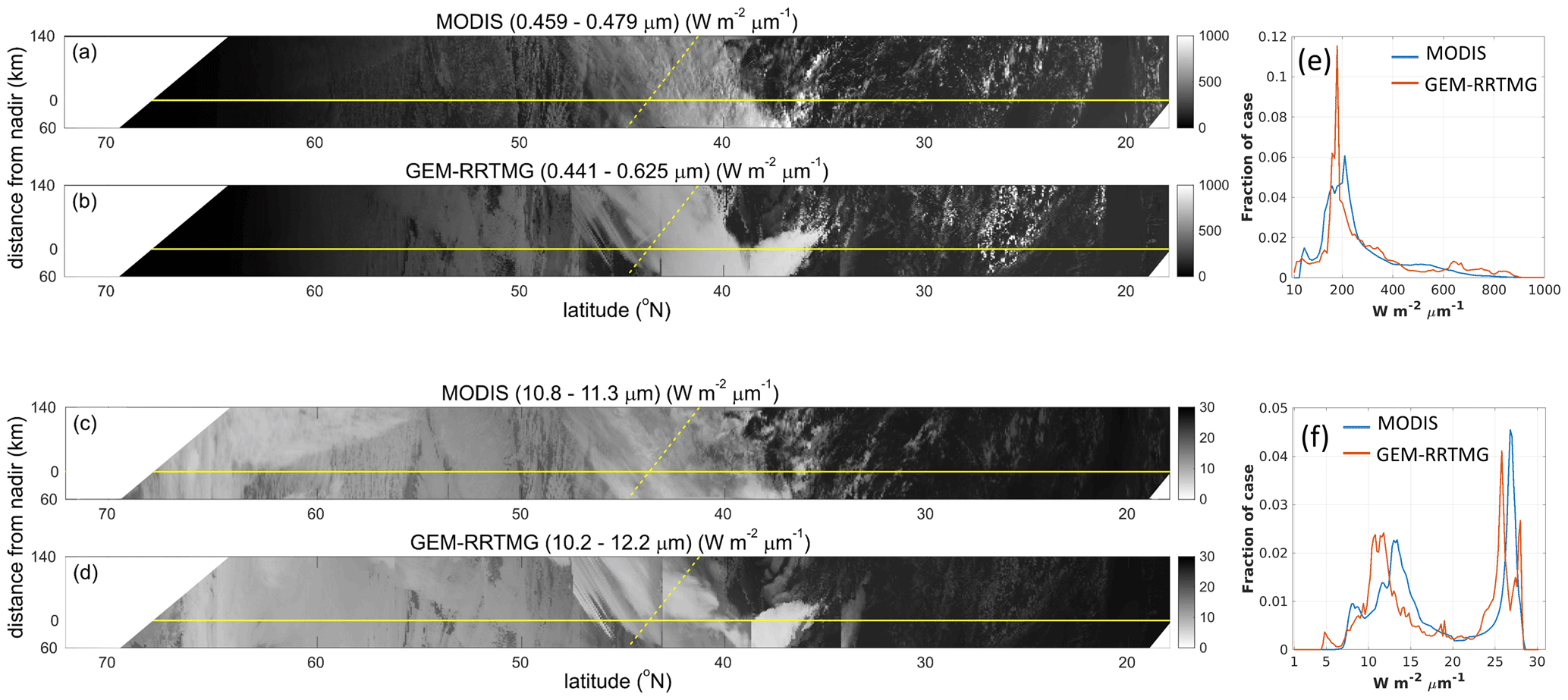
Figure 8 (a) MODIS TOA flux (approximated by radiance times π) for band 3 (459–479 nm) between 17:15 and 17:35 UTC on 7 December 2014. (b) RRTMG simulated upward TOA flux for 441.5–625 nm for GEM's simulation of the Halifax frame. Panel (c) as in (a) but for band 31 (10.8–11.3 µm). Panel (d) as in (a) but for 10.2–12.2 µm wavelengths. Solid and dashed yellow lines indicate EarthCARE's and CloudSat's nadir tracks. Blank areas are outside MODIS's field-of-view. (e) Frequency distributions of fluxes for band 3 (bin size of 10 $\mathrm{W}{\mathrm{m}}^{-\mathrm{2}}\mathrm{\mu }{\mathrm{m}}^{-\mathrm{1}}$). Panel (f) as in (e) but this is for band 31 (bin size of 0.2 $\mathrm{W}{\mathrm{m}}^{-\mathrm{2}}\mathrm{\mu }{\mathrm{m}}^{-\mathrm{1}}$).

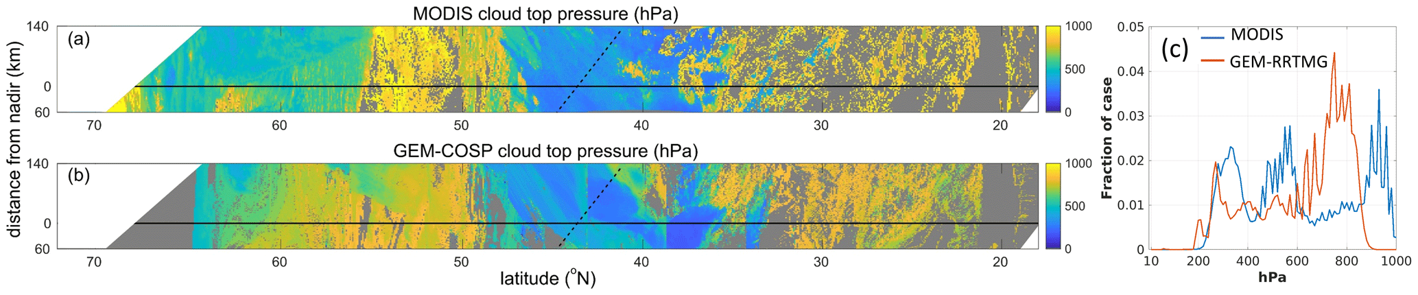
Figure 9 (a) MODIS cloud top pressure (MYD06_L2 product) between 17:15 and 17:35 UTC on 7 December 2014. Blank areas are outside MODIS's field-of-view. (b) GEM's cloud top pressure for the Halifax frame is based on COSP's MODIS simulator. Gray area in the northern portion has ${\mathit{\theta }}_{\mathrm{0}}>\mathrm{90}{}^{\circ }$ and so no COSP values. (c) Frequency distributions of cloud top pressure (bin size of 10 hPa).

Near 38^∘ N GEM's longwave fluxes are significantly less than MODIS's fluxes. This is because GEM simulated widespread convection in this area, whereas MODIS only observed isolated convective cells. This is also evident in Fig. 8e and f as GEM shows higher frequencies around 820 and 5 $\mathrm{W}{\mathrm{m}}^{-\mathrm{2}}\mathrm{\mu }{\mathrm{m}}^{-\mathrm{1}}$, respectively. This is also apparent in Fig. 9, which shows cloud top altitudes both inferred from MODIS radiances (Platnick et al., 2015) and computed by the MODIS simulator of the Cloud Feedback Model Intercomparison Project (CFMIP) Observation Simulator Package (COSP; Bodas-Salcedo et al., 2011).

GEM's cloud top altitudes are too high for low clouds between latitudes 20 and 30^∘ N and 50 and 55^∘ N; most are near 750 hPa, whereas MODIS's values are mostly near 920 hPa. This can also be inferred from Fig. 8f in which higher frequencies of infrared spectral fluxes from GEM are found between 23 and 25.5 $\mathrm{W}{\mathrm{m}}^{-\mathrm{2}}\mathrm{\mu }{\mathrm{m}}^{-\mathrm{1}}$ for the southern section and between 10 and 12 $\mathrm{W}{\mathrm{m}}^{-\mathrm{2}}\mathrm{\mu }{\mathrm{m}}^{-\mathrm{1}}$ for the northern section. Additionally, Fig. 9c shows that GEM underestimates the number of mid-level clouds between 500 and 600 hPa in the region between latitudes 55 and 62^∘ N.

These above-mentioned differences cannot be explained by the slight time difference between MODIS observation (∼ 17:20 UTC) and GEM simulation time (17:30 UTC). On the other hand, it is common for NWP models to simulate some characteristics of cloud systems quite well yet show temporal/spatial displacements relative to observations (e.g., Qu et al., 2018). The goal when simulating these test scenes was, however, to produce large, well-resolved tracts of realistic clouds; an emphasis on exactly what happened was secondary.

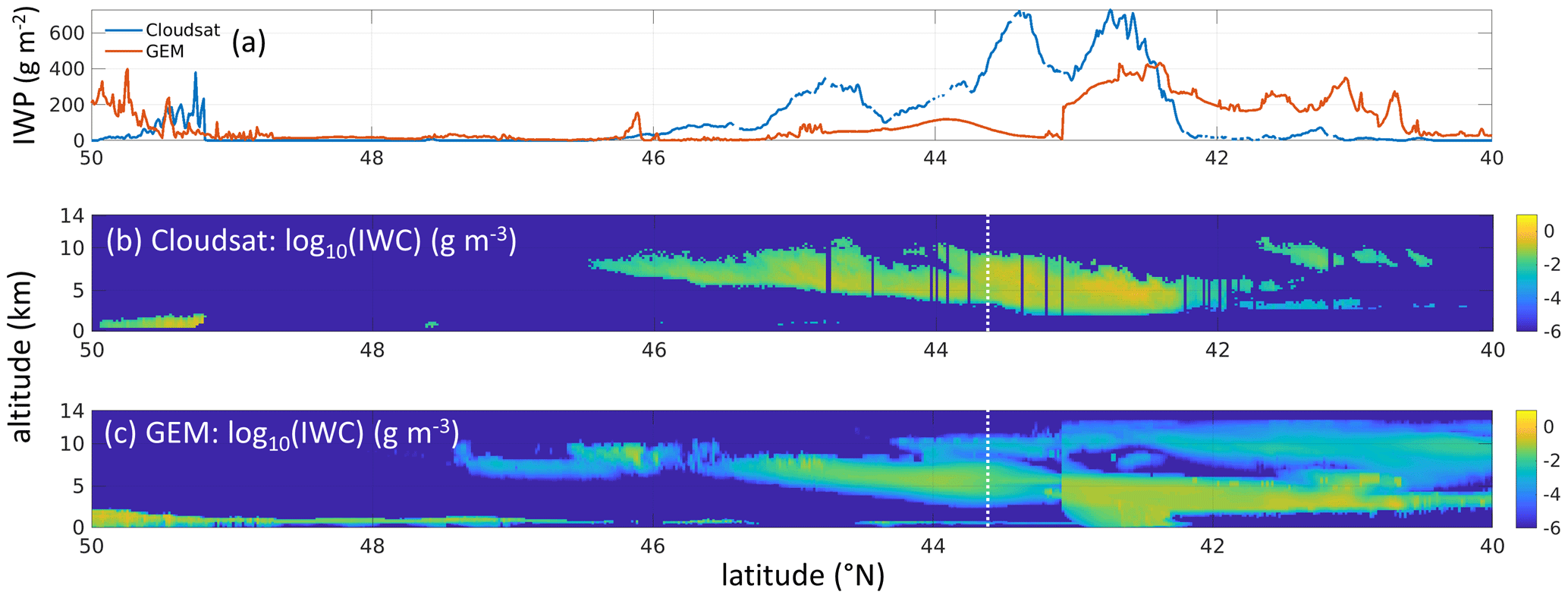
Figure 10 (a) Ice water path (IWP) inferred from CloudSat observations at 17:21 UTC on 7 December 2014 as it crossed the Halifax frame between latitudes 41–44^∘ N (dashed yellow line in Fig. 8) and as simulated by GEM along the nadir track (solid yellow lines in Fig. 8). Panels (b) and (c) are ice CWC for CloudSat and GEM, respectively. Dashed white line indicates where CloudSat's and EarthCARE's tracks intersected.

Figure 10b and c show cross sections of ice CWC inferred from CloudSat radar reflectivities and simulated by GEM, respectively (for the transect indicated in Fig. 8). While the cross sections intersect only at latitude 43.6^∘ N, the general forms of the fields agree well and not just in the immediate vicinity of the intersection point. Between 42 and 43^∘ N, GEM produces a large amount of solid precipitation, whereas in CloudSat data, due to the ground clutter, there is no reliable retrieval available. Unfortunately, CloudSat's retrieval of liquid CWC is problematic (e.g., Li et al., 2018) and is not used here to assess GEM's retrieval. Figure 10a shows the values of ice water path (IWP) which are vertical integrals of values in Figure 10b and c. At and around the intersection point, CloudSat's IWP values are much larger than GEM's, but again, the forms of their curves are fairly similar. The edge of GEM's inner-domain near 43^∘ N is abundantly clear.

6.2 Baja frame

Figure 11 compares MODIS TOA fluxes to those computed by RRTMG acting on GEM data for the Baja frame. As with the Halifax frame, agreement is generally good, though GEM's fields exhibit some peculiarities. For instance, GEM's fluxes associated with clouds are less variable than MODIS's, especially between 40 and 50^∘ N. This could be due to both GEM's clouds being simply too homogeneous due to missing mesoscale forcing (Stensrud and Gao, 2010) or RRTMG's use of 1D radiative transfer models (Barker et al., 2017). Also, the thin high clouds near latitude 32^∘ N, which are also evident in Fig. 12 and positioned well in space, show an on–off pattern that is not seen in the observations. Furthermore, near latitude 55^∘ N GEM failed to produce the very thin, but extensive, clouds below 800 hPa. This is most apparent in Fig. 12. GEM's overestimation of cloud tops close to 400 hPa near latitude 50^∘ N is consistent with Figs. 12c and 11e and f, which show significant overestimations of fluxes between 620 and 730 $\mathrm{W}{\mathrm{m}}^{-\mathrm{2}}\mathrm{\mu }{\mathrm{m}}^{-\mathrm{1}}$ for the visible band and between 7 and 10 $\mathrm{W}{\mathrm{m}}^{-\mathrm{2}}\mathrm{\mu }{\mathrm{m}}^{-\mathrm{1}}$ for the infrared band. Note too that the discontinuities that stem from stitching together GEM's innermost domains are less apparent for this frame than they are for the Halifax frame, though the discontinuity near 26^∘ N is notably bad for it stands out in both visible and IR imagery.

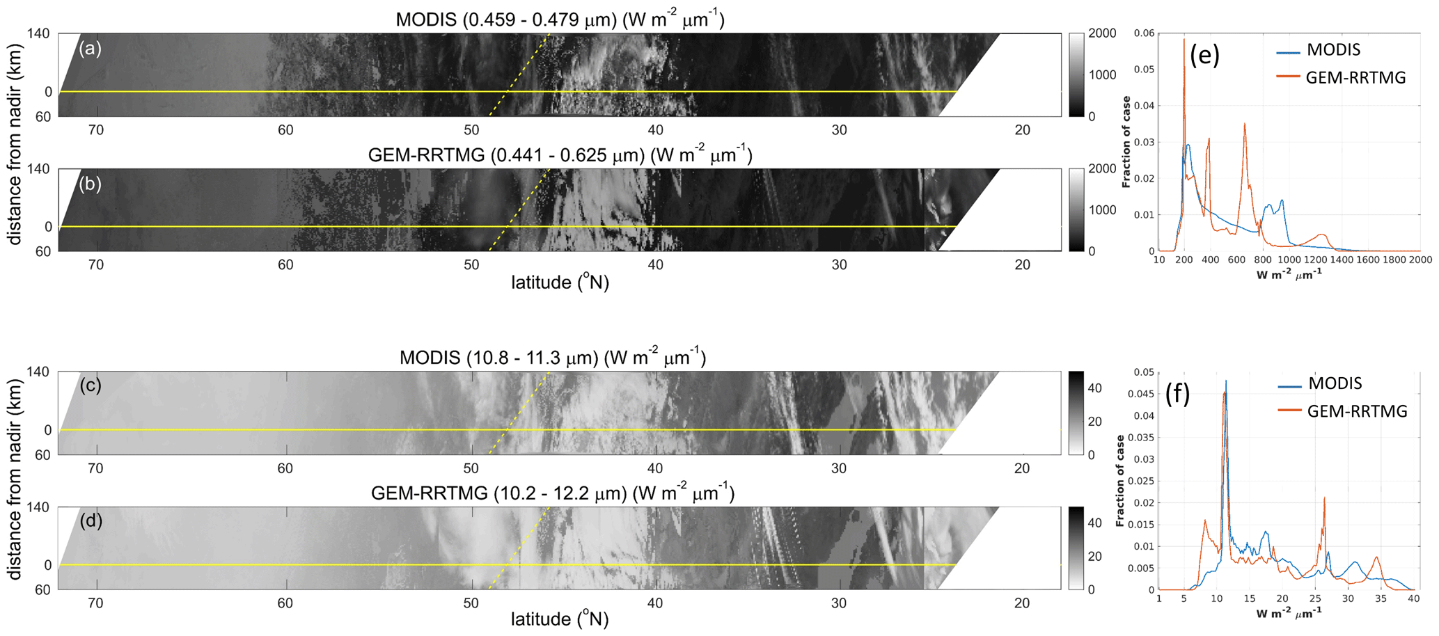
Figure 11 As in Fig. 8 except these are for the Baja frame. MODIS observations were between 20:10 and 20:30 UTC on 2 April 2015.

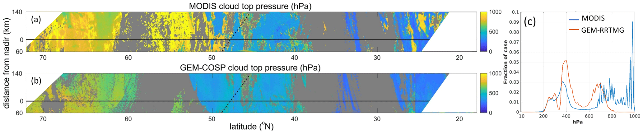
Figure 12 As in Fig. 9 except these are for the Baja frame. MODIS cloud top pressures are retrieved between 20:10 and 20:30 UTC on 2 April 2015.

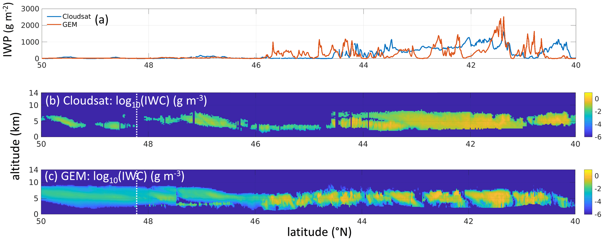
Figure 13 As in Fig. 10 except these are for the Baja frame. CloudSat's track indicated by the dashed yellow line in Fig. 11 is between latitudes 45–49^∘ N.

Despite these discrepancies, Fig. 13 shows that in the vicinity of where the satellite tracks intersect, vertical realizations of clouds from both GEM simulations and CloudSat retrievals indicate smooth mid-level low-density clouds, although GEM's are more extensive. The altitudes of GEM's clouds over the Rocky Mountains are also in fair agreement with CloudSat's altitudes. Unlike the Halifax frame, the magnitudes of modeled and “observed” IWPs agree quite nicely, in general.

6.3 Hawaii frame

Figure 14 shows that for the Hawaii frame, GEM's positionings and approximate intensities of cloud systems near the Equator and ∼25^∘ S agree well with the MODIS observations. The harsh discontinuity in GEM's string of innermost domains near 2^∘ S is due to a lack of high ice cloud, as seen in Fig. 15, which likely stems from the lack of information, in the form of reduced outflow of high cirrus coming into the sub-domain from the equatorial mesoscale system. Likewise, near 15^∘ N the lack of upper-level cloud in GEM could be because this sub-domain was too disconnected from the mesoscale system to the south. The lack of high cloud in the simulation can be inferred from Fig. 14e which shows an overabundance of fluxes by GEM near 200 $\mathrm{W}{\mathrm{m}}^{-\mathrm{2}}\mathrm{\mu }{\mathrm{m}}^{-\mathrm{1}}$, a value that resembles TOA visible fluxes from ocean surface. This is also seen in Figs. 14f and 15c. Again, however, the point of this section is to show the gross verisimilitude of the test frames and hence their suitability for EarthCARE algorithm assessments.

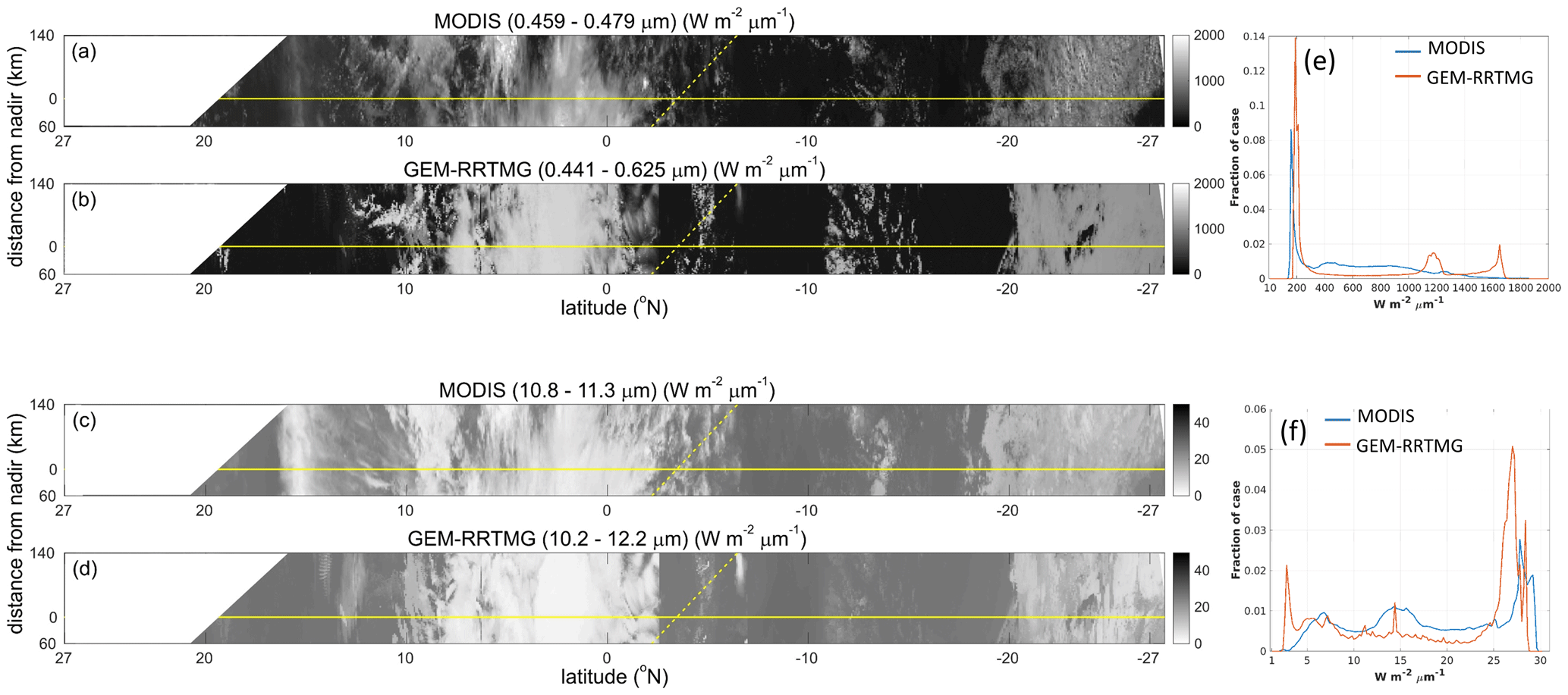
Figure 14 As in Fig. 8 except these are for the Hawaii frame. MODIS observations were between 00:35 and 00:55 UTC on 24 June 2015.

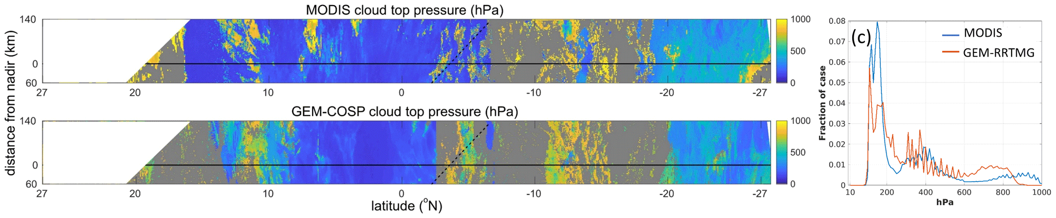
Figure 15 As in Fig. 9 except these are for the Hawaii frame. MODIS cloud top pressures were retrieved from observations between 00:35 and 00:55 UTC on 24 June 2015.

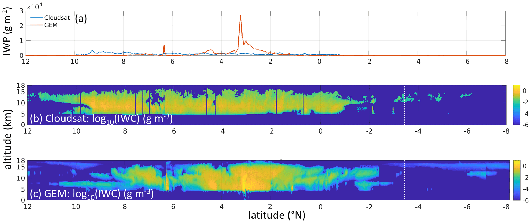
Figure 16 As in Fig. 10 except these are for the Hawaii frame. CloudSat's track indicated by the dashed yellow line in Fig. 14 is between latitudes 1.5–6.5^∘ S.

As Fig. 16 shows, despite CloudSat's track intersecting EarthCARE's well south of the mesoscale system situated near the center of the Hawaii frame, the system was sufficiently large in the zonal direction that CloudSat's sampling of it can be compared to EarthCARE's sampling of GEM's simulations. The regions of high ice CWC values for the two samples match extremely well both vertically and horizontally. The distribution of ice CWC inferred from CloudSat reflectivities is very narrow, while GEM's is much broader with many extremely small values (10⁻⁴ to 10⁻⁵ g m⁻³) that are below the detection threshold of COSP. Aside from the huge spike in IWP for GEM near 3^∘ N, which obviously included some precipitation, the magnitude and forms of the curves for CloudSat and GEM agree well.

What might appear to be a deficiency with GEM is the extreme lack of texture in the visible reflectance of cloud associated with the frontal system in the south of the frame. As with the other frames, however, it is entirely likely that the smoothness of GEM's field stems from the application of a 1D radiative transfer model (see Barker et al., 2017). This is addressed explicitly in other papers in this special issue (Cole et al., 2023).

7 Alterations of GEM's ice crystal sizes

As GEM's scenes are to be input to ECSIM (Voors et al., 2007) to simulate synthetic L1 measurements for ATLID, CPR, MSI, and BBR (Donovan et al., 2023), it is important not only that macrophysical cloud properties be realistic for phenomena such as solar RT and CPR nonuniform beam filling (Tanelli et al., 2002), but that cloud microphysical properties, such as size distributions and mass–diameter relationships, be as well. While the macrophysical cloud properties simulated by GEM were deemed satisfactory in the previous section, it was clear that there were shortcomings with its predicted ice cloud microphysical properties (see Qu et al., 2018). These deficiencies had a demonstrably negative impact on the realism of ECSIM's simulated measurements, and so adjustments to ice particle sizes were needed.

Basically, GEM predicts too many overly small ice crystals with R_eff<10 µm. The cause of this appears to be overestimation of ice crystal number concentrations near cloud tops. Currently, secondary ice production (SIP) mechanisms are poorly understood (Field et al., 2017; Korolev and Leisner, 2020), and while at least six SIP mechanisms are known (Korolev et al., 2020), only the Hallett–Mossop process (Hallett and Mossop, 1974; Mossop and Hallett, 1974) is parametrized in the MY2 scheme. It appears as though ice number concentrations in GEM's simulations are systematically underestimated near, or just above, the melting layer. Hence, cloud glaciation times will be too long, and an excess of liquid droplets will be sent too high by updrafts. In the current scheme, droplets will eventually be converted into ice crystals via homogenous freezing, and this will produce very high concentrations of small crystals at altitude. While ongoing studies aim to improve representations of SIP (e.g., Huang et al., 2021; Qu et al., 2022a), they are not yet ready for use in GEM. As such, more manual alterations to GEM's ice crystal sizes were needed.

To improve the realism of the synthetic observations, the following adjustments were made to GEM's original fields:

1. Implicit liquid CWCs (see Table A1 in the Appendix) at temperatures<273 K were set to zero, thereby reducing unrealistically large numbers of super-cooled droplets.

2. Implicit ice CWCs (see Table A1 in the Appendix) were removed because crystal R_eff was artificially fixed at 15 µm.

3. The mass–dimension relationships used by GEM for ice and snow were replaced by those described in Erfani and Mitchell (2016), and the functional form of ice particle size D distribution was changed. Specifically, it was altered by multiplying by a factor of D⁴, which had the effect of increasing mean D. Following these adjustments, particle number densities were recalculated subject to the conservation of GEM's original total ice and snow water contents.

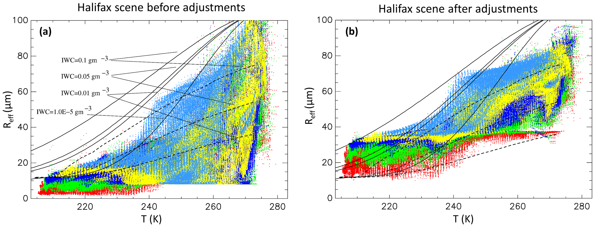
Figure 17 Effective radius R_eff as functions of temperature for GEM's results both before and after application of adjustments discussed in the text. R_eff is defined in terms of the mass and cross-sectional area of crystals following Donovan and van Lammeren (2001). Solid lines in the “before” panel correspond to the parametrization described in Wyser (1998), while dotted lines follow Donovan and van Lammeren (2002). Colors of dots correspond to different ranges of ice water content (IWC) (g m⁻²) (red: IWC<0.0001; green: $\mathrm{0.0001}<\text{IWC}<\mathrm{0.001}$; blue: $\mathrm{0.001}<\text{IWC}<\mathrm{0.01}$; yellow: $\mathrm{0.01}<\text{IWC}<\mathrm{0.1}$; and light blue: 0.1<IWC).

These alterations were found to produce significant, albeit from a qualitative perspective, improvements to GEM's simulated cloud properties. For example, considering the issue of too many ice crystals that are too small, Fig. 17 shows the relationship between cloud and ice particle R_eff before and after the adjustments listed above. It can be seen that the population of small crystals at temperatures above 245 K has been eliminated, whilst below 240 K, minimum particle sizes after adjustments exceed 10 µm. Moreover, the distribution of R_eff after adjustments is more consistent with the phase space indicated by real observations (e.g., Donovan and van Lammeren, 2001; Wyser, 1998). Lines in Fig. 17 are from parametrizations. While many observation-based parametrizations of ice crystal size distribution exist, they exhibit only moderate agreement, and so cannot be used to fully support the credibility of adjusted R_eff. It can be concluded, however, with some certainty, that the above adjustments removed unrealistically small ice crystals and that the resulting temperature distribution of R_eff is in fair agreement with observations.

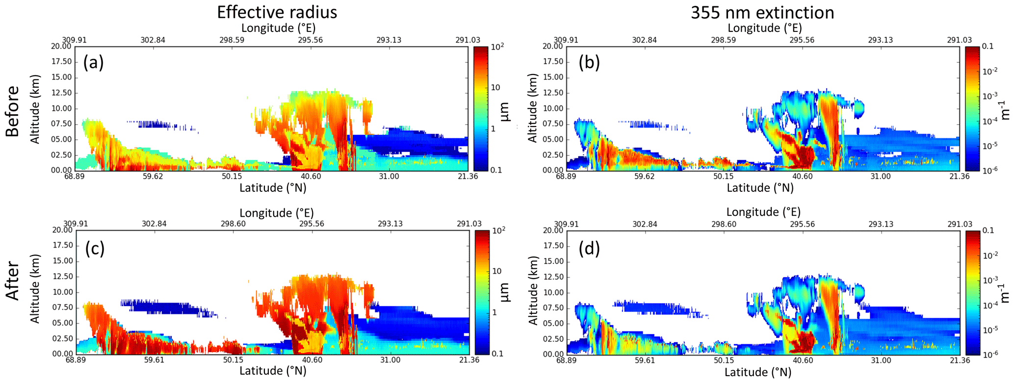
Figure 18 Nadir cross sections of R_eff and 355 nm extinction before and after making adjustments described in the text. Note that the changes in the aerosol regions, e.g., the elevated layer north of 50^∘ at around 7 km, are due to technical updates to the aerosol processing between the “before” and “after” data not related to the ice cloud adjustments.

Censoring the implicit super-cooled liquid and ice water, as well as the adjustment to ice and snow R_eff, has important consequences for the vertical structure of optical extinction. This can be seen in Fig. 18 where nadir cross sections of R_eff and extinction at 355 nm (the operating wavelength of ATLID) are shown both before and after adjustments were performed. Increases in R_eff and droplet extinction for clouds poleward of 50^∘ N and at altitudes below 5 km stem from a combination of removing super-cooled implicit water and increases to ice and snow R_eff. The reduction in cloud extinction, especially near cloud tops between 35 and 45^∘ N, is mainly a consequence of increasing R_eff of ice particles.

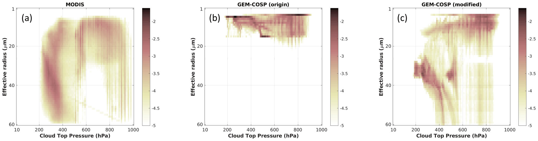
Figure 19 Histograms showing number of cases in logarithmic scale as functions of effective radius (bin width of 1 µm) and cloud top pressure (bin width of 10 hPa). (a) MODIS retrievals from MYD06_L2 product. (b) Original GEM data simulated by MODIS simulator of COSP. Panel (c) as in (b) but this is for adjusted effective radii.

Impacts of these adjustments can be seen in Fig. 19, which shows fractions of cases as functions of effective radius and cloud top pressure. Figure 19a is for MODIS retrievals (MYD06_L2) and shows that for most cases with cloud top pressure between 200 and 400 hPa effective radii are between 30 and 50 µm. Figure 19b shows that for COSP simulations based on GEM data, most ice clouds for the same cloud top pressures have an effective radius smaller than 15 µm. After applying the adjustments, however, COSP values improve significantly with most effective radii between 30 and 50 µm. Though not shown, similar impacts exist for the Baja and Hawaii scenes.

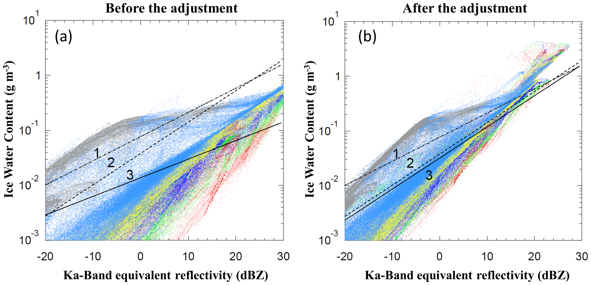
Figure 20 IWC vs. Ka-band equivalent reflectivity for the nadir track of the Halifax scene. Lines 1 and 2 are best-fit lines to GCPEX and CRYSTAL-FACE data, respectively (see Matrosov and Heymsfield, 2017). Line 3 is best-fit to GEM results. Red points are for temperatures T (in ^∘C) between 0 and −5 ^∘C, green $-\mathrm{10}<T<-\mathrm{5}$ ^∘C, dark blue $-\mathrm{15}<T<-\mathrm{10}$ ^∘C, yellow $-\mathrm{20}<T<-\mathrm{15}$ ^∘C, light blue $-\mathrm{40}<T<-\mathrm{20}$ ^∘C, and gray $T<-\mathrm{40}$ ^∘C. Panel (a) is for before adjustment of effective radii, and (b) is for after adjustment.

In addition to these improvements in cloud optical properties, the same adjustments were found to improve the realism of cloud properties that are relevant for the simulation of CPR observations. For example, after applying the adjustments the relationship between ice CWC and simulated radar reflectivity now falls in phase space, which agrees well with real observations (e.g., Matrosov and Heymsfield, 2017; Heymsfield et al., 2005). Figure 20 shows the ice water content (IWC) vs. Ka-band reflectivity for the nadir Halifax scene path. It can be seen that after adjustment (Fig. 20b) the best-fit line of GEM data compares well with the relationships shown in Fig. 4 of Matrosov and Heymsfield (2017). The agreement is even more striking when distributions of data shown in Matrosov and Heymsfield (2017) are considered instead of just best-fit lines. Various cross sections of adjusted GEM- and CAMS-derived fields can be found in the Supplement.

8 Conclusions, perspectives, and data availability

In this day and age, it is difficult to see how a scientifically and technically advanced research satellite could be launched without having first completed a pre-launch end-to-end numerical simulation program that assesses myriad aspects of mission performance and demonstrates the likelihood of achieving the mission's science goals. Such a program would begin with the simulation of atmosphere–surface conditions that ideally span, and resemble, much of what can be expected to be encountered during the mission. Virtual observations, to be made by the satellite's sensors, are then simulated for the mock atmosphere–surfaces, and they are, in turn, operated on by retrieval algorithms. This exact end-to-end simulation program has unfolded, over the past 2 decades, for the EarthCARE satellite mission (ESA, 2001; Illingworth et al., 2015). The purpose of this paper was to summarize the atmosphere–surface test datasets.

The synthetic atmosphere–surface systems used for this study were produced by ECCC's Global Environment Multiscale model, which is abbreviated as “GEM” (Côté et al., 1998; Girard et al., 2014). This operational numerical weather prediction model is well-known internationally (Leroyer et al., 2014, 2022; Bélair et al., 2017; Milbrandt et al., 2016; Qu et al., 2018, 2020, 2022a; McTaggart-Cowan et al., 2019). The end-to-end program was intended initially to test retrieval algorithm performance but was expanded to address ESA's communication and data-handling segments, too. As such, large simulated domains were required. The fundamental data processing element is referred to as a “frame”. There are eight frames per orbit, and so simulated “test frames” had to be ∼6200 km along-track. The across-track swath of EarthCARE's multispectral imager (MSI) is 150 km, and so test frames had to be at least this wide, but to avoid edge-effects, their widths were extended to 200 km. Horizontal and vertical resolutions for GEM's simulations had to allow for at least some variability within the footprints of EarthCARE's sensors. The use of 57 vertical layers and horizontal grid spacing of Δx of 0.25 km was deemed adequate (see Qu et al., 2018).

Three test frames, which followed orbits provided by ESA, were identified via examination of satellite data and available surface weather observations. Conditions that were captured include a cold frontal system; broken shallow cumulus; a tropical mesoscale convective system; thin cirrus; multi-layer clouds; and clear-sky conditions, with aerosols, over ocean, land (including mountains), and ice–snow surfaces. Surface bidirectional reflection distribution functions (BRDFs) and albedos from climatological data and aerosol properties were added to GEM's simulations. GEM's computational Equator was oriented along each EarthCARE orbit, and a set of nested simulations were performed that culminated in 13 separately simulated innermost domains at Δx=0.25 km. These domains were concatenated to form the full 6200 km test frames.

It was discovered that GEM's descriptions of some ice cloud properties lack the realism needed for adequate simulation of virtual observations and assessment of cloud and aerosol property retrieval algorithms. Hence, modifications were made to the effective size of ice particles based on surface and in situ observations. Most of the important impacts were to particle sizes near cloud tops.

Previous studies have simulated atmospheric conditions for purposes of satellite algorithm development and evaluation (e.g., MPB Technologies Inc., 2000; Voors et al., 2007; Tao et al., 2009), constraint of cloud microphysical schemes by observations (Matsui et al., 2013; Iguchi et al., 2012a, b, 2014), and assimilation of retrieved aerosol properties into NWP models (Zeng et al., 2020; Cornut et al., 2023), but the simulations done for this study had to serve several purposes simultaneously, and this put unique demands on them. Most notably was their size, for they had to provide sufficient detail to meet several wide-ranging aspects of observation simulation and algorithm assessment, with enough areal extent to evaluate data processing and archiving procedures.

As such, the overarching requirement placed on the time-sensitive production of these test frames was that they be deemed, by myriad mission researchers and managers, “sufficiently” realistic and “necessarily” expansive enough to provide adequate assessment of the numerous key steps that will be required to produce EarthCARE data. No doubt, this requirement compromised some aspects of both the quality of the simulations and their verification against independent sources of information. Moreover, efforts are being made to improve upon these test data. In particular, the two-moment bulk cloud microphysics scheme Predicted Particle Properties (P3) (Morrison and Milbrandt, 2015; Milbrandt and Morrison, 2016; Cholette et al., 2019; Qu et al., 2022h) is being used.

That said, it is felt roundly that the objectives behind the test frames have been realized and that they have the potential to be used for other observation missions that could include platforms other than satellites, particularly those targeting cloud, aerosol, and radiation interactions. The full dataset is available publicly as summarized in the “Data availability” section at the end. It includes atmospheric and surface properties produced by GEM data, modified hydrometeor properties, climatological surface optical properties, and the properties of added aerosols (see tables in the Appendix).

Appendix A: List of test frame variables

Table A1 Variables for the original GEM simulations.

Table A2 Variables archived for the test frames.