the Creative Commons Attribution 4.0 License.
the Creative Commons Attribution 4.0 License.
 | 02 Nov 2023
Statistical assessment of a Doppler radar model of TKE dissipation rate for low Richardson numbers
Lakshmi Kantha
Hiroyuki Hashiguchi
The potential ability of VHF or UHF Doppler radars to measure turbulence kinetic energy (TKE) dissipation rate ε in the atmosphere is a major asset of these instruments because of the possibility to continuously monitor turbulence in the atmospheric column above the radars. Several models have been proposed over the past decades to relate ε to half the Doppler spectral width σ, corrected for non-turbulent contributions, but their relevance remains unclear. Recently, Luce et al. (2023) tested the performance of a new model expected to be valid for weakly stratified or strongly sheared conditions, i.e., for low Richardson (Ri) numbers. Its simplest expression is εS=CSσ2S, where CS∼0.64 and is the vertical shear of the horizontal wind V. We assessed the relevance of this model with a UHF (1.357 GHz) wind profiler called WPR LQ-7, which is routinely operated at the Shigaraki Middle and Upper Atmosphere (MU) observatory (34.85∘ N, 136.10∘ E) in Japan. For this purpose, we selected turbulence events associated with Kelvin–Helmholtz (KH) billows, because their formation necessarily requires Ri<0.25 somewhere in the flow, a condition a priori favorable to the application of the model. Eleven years of WPR LQ-7 data were used for this objective. The assessment of εS was first based on its consistency with an empirical model , where Lout has the dimension of an outer scale of turbulence. It was found to compare well in a KH layer with direct estimates of ε from in situ measurements for Lout≈70 m. Some degree of equivalence between εS and εLout was confirmed by statistical analysis of 192 KH layers found in the height range 0.3–5.0 km indicating that , where is the Hunt scale defined for neutral turbulence. The degree of equivalence is even significantly improved if Lout is not treated as a constant but depends on the depth D of the layer. We found Lout≈0.0875D or equivalently LH∼0.056D, which also means that σ is proportional to the apparent variation in the horizontal velocity (S×D) over the depth of the KH layer. Consequently, εS=0.64σ2S and would express the same model for KH layers when Ri remains low. For such a condition, we provide a physical interpretation of εLout, which would be qualitatively identical to that for neutral boundary layers.
- Article
(1478 KB) - Full-text XML
- BibTeX
- EndNote


VHF stratosphere–troposphere (ST) radars and UHF wind profilers can be used to estimate the turbulence kinetic energy (TKE) dissipation rate ε in the atmosphere, from half the Doppler spectral width corrected for non-turbulent effects (hereafter, denoted by σ) (e.g., Hocking, 1983; Doviak and Zrnić, 1984; Hocking et al., 2016 and references therein). If the measurements are made with a zenith-pointing beam as is the case in the present paper, σ2 is expected to be an estimate of the variance 〈w′2〉 of the vertical component of wind fluctuations produced by turbulence. Luce et al. (2023) (hereafter L2023) tested three radar models relating σ2 to ε using data collected by a UHF wind profiler called WPR-LQ-7 (Imai et al., 2007), and routinely operated at Shigaraki MU Observatory (34.85∘ N, 136.10∘ E) in Japan. The models require determination of the non-dimensional gradient Richardson number , where (s−1) is the vertical shear of the horizontal wind and where (where θ is the potential temperature and g is gravitational acceleration) is the square Brunt–Vaïsälä or buoyancy frequency. Comparisons with direct estimates of ε obtained from in situ measurements with turbulence sensors aboard fixed-wing DataHawk unmanned aerial vehicles (UAVs, Lawrence and Balsley, 2013; Kantha et al., 2017) in the altitude range 0.3–4.5 km led to two findings. (1) An empirical model with Lout∼70 m provides the best statistical agreement with in situ estimates (Fig. 5 of L2023) confirming results obtained by Luce et al. (2018) (their Fig. 9) with the VHF MU radar. (2) The model εS=CSσ2S provides better agreement than εN=CNσ2N. εN is commonly used by the mesosphere–stratosphere–troposphere (MST) radar community. It is expected to be applicable to turbulence under stable stratification (e.g., Hocking, 1983; Hocking et al., 2016). εS was proposed originally by Hunt et al. (1988) from heuristic arguments and confirmed by Basu et al. (2021) and Basu and Holtslag (2022) from direct numerical simulations (DNS) and analytical derivations. It is expected to be valid for weakly stratified and/or strongly sheared conditions, i.e., for low Ri values. Unlike εS, no conditions on N or Ri have been established for εN to be valid (except that N2 must be positive). Clearly, εN is not valid for neutral stratification.
L2023 showed that εS gives statistical results that are “intermediate” to εLout and εN. As turbulence is expected to occur and to be maintained mainly when Ri is low, this property should favor the validity of εS over εN if εS is a relevant model. To ascertain this, we need to check the model under the conditions for which it is supposed to be valid, i.e., when Ri is low (less than roughly 0.2), according to the DNS of Basu et al. (2021). Ri cannot be estimated from the radar data alone because N2 is not measurable by radar (except when the air is dry and stable, i.e., possibly in the stratosphere, Luce et al., 2007). It is usually obtained from measurements of pressure and temperature and winds by meteorological radiosondes. However, radiosonde measurements are scarce and rarely co-located with radar measurements. In addition, Ri is a scale-dependent parameter (e.g., Balsley et al., 2008) and there is no prescribed method to calculate the appropriate value of Ri, making it difficult to apply quantitative criteria to Ri for a selection of cases to be studied. For the present study, we used an alternative strategy that avoids these difficulties, the goal being to find out if, not when, εS can actually be relevant for low Ri values. The most favorable condition for this goal is Kelvin–Helmholtz (KH) billows. Indeed, these structures are produced by shear instabilities, which grow when is met somewhere in the flow and are generally associated with enhanced turbulence. They are also clearly visible in radar echoes, and hence easily identified and earmarked for further study. L2023 evaluated the performance of the radar models for a KH layer (i.e., a turbulent layer exhibiting KH billows) of ∼800 m in depth sampled several times by a DataHawk during the 2017 Shigaraki UAV Radar Experiment (ShUREX). They found that both εLout with Lout∼70 m and εS provide values consistent with DataHawk-derived ε. This result is the cornerstone of the reasoning that we will follow in this paper. If it is representative, this will provide a physical interpretation of the empirical model when applied to turbulence produced by a KH instability. Therefore, we tried to answer the following question: to what extent is the equivalence between εS and εLout also observed for other KH events? For this purpose, we searched for KH layers in time–height cross-sections of WPR LQ-7 echo power from 2011 to 2021. We identified 192 cases that could be easily analyzed. They allowed us to verify and qualify the result stated by L2023 by taking into account the influence of the depth D of the KH layers and to infer a relationship between the Hunt scale LH defined as and D.
Section 2 describes the main characteristics of WPR LQ-7 and the parameters used for routine observations. Section 3 briefly introduces the εS model and the results of the case study described by L2023. Section 4 presents the method and criteria used for the KH layer selection. Section 5 shows the statistical results for 192 KH layers identified, and for 113 turbulent KH layers selected more subjectively for analysis. Finally, conclusions are given in Sect. 6.
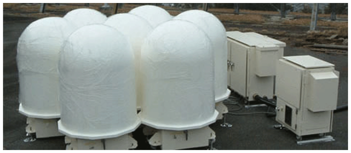
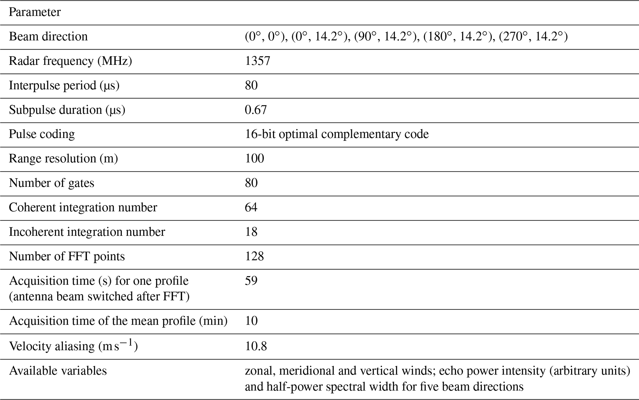
The WPR LQ-7 is a 1.3575 GHz Doppler radar. It has a phased array antenna composed of seven Luneberg lenses of 800 mm diameter (Fig. 1). Its peak output power is 2.8 kW. It can be oriented in five directions sequentially (i.e., after fast Fourier transform (FFT) operations), vertically and 14.2∘ off zenith toward the north, east, south and west. The main radar parameters of the WPR-LQ-7, installed at Shigaraki MU Observatory and in operation since 2006, are given in Table 1. The acquisition time for one profile composed of 80 altitudes from 300 m above ground level every 100 m in each direction after 18 incoherent integrations is 59 s but for a total of 11.8 s of observations for each direction (due to overlapping directions). The time series are processed by automatic algorithms to remove outliers (e.g., bats, birds, airplanes) and ground clutter as much as possible. Low signals near and below the detection thresholds are removed. Profiles of variables (zonal, meridional and vertical winds; echo power in arbitrary units; half-power spectral width 2σmeas(1/2) related to σmeas by , where 2σmeas is the measured Doppler spectral width) averaged over 10 min are made available for routine monitoring (http://www.rish.kyoto-u.ac.jp/radar-group/blr/shigaraki/data/, last access: 28 October 2023). Because of the high-quality data control, the 10 min averaged data are used to retrieve ε with the goal of assessing these routine data for further analyses.
3.1 Description
For low gradient Richardson numbers, several studies showed from heuristic arguments that ε can be written as (Hunt et al., 1988; Schumann and Gerz, 1995)
where 〈w′2〉 is the variance of the vertical wind fluctuations produced by turbulence and CS is a constant. Equation (1) is equivalent to , where is the Hunt scale. The Hunt scale describes the maximum size of the turbulent eddies, which are stretched and destroyed by the wind shear. In strongly sheared or weakly stratified flows, eddies can be affected first by the wind shear before being affected by the stratification. Hunt et al. (1988) suggested that Eq. (1) can be valid up to Ri ∼0.5. Schumann and Gerz (1995) found that it can be valid up to Ri∼1 from large eddy simulations (LES).
From simplified budget equations for TKE and temperature variance, and using similarity theory, Basu and Holtslag (2022) evaluated the constant CS to be 0.64 and provided a generalization of Eq. (1):
where Rf is the flux Richardson number. For Ri→0, Rf→0, then , i.e., Eq. (1) with CS=0.64. From DNS, Basu et al. (2021) found Eq. (1) with CS=0.60 for Ri up to at least 0.2. L2023 put in perspective εS and the commonly used model , which can be re-written as , where is the buoyancy scale. LB is a measure of the eddy scale at which vertical turbulent motions are suppressed. By definition, when Ri<1, LH<LB and vice versa. It is then quite logical to assume that, when Ri≪1, stratification effects can be neglected and εS is more appropriate than εN. In the Appendix, we propose the corresponding equation of heat diffusivity for low Ri values, when Eq. (2) is valid.
If σ2 can be assimilated to 〈w′2〉, then εS can be evaluated from the radar data alone, since an estimate of S can be obtained at the range and time resolutions of the radar. Equation (1) was applied by Fukao et al. (2011) to KH layers detected by the 46.5 MHz MU radar but with a coefficient different from 0.64 and not for the right reason. This was to compensate for the lack of N2 measurements, assuming that εN was the appropriate model.
3.2 The case study
Figure 2a shows the time–height cross-section of signal-to-noise ratio (SNR, in dB) at vertical incidence on 18 June 2017 from 13:30 to 16:30 LT and between 0.3 and 7 km altitude (above sea level) at a time resolution of 59 s. A KH layer of about 800 m in depth associated with enhanced SNR is clearly visible around the altitude of ∼ 3.0 to ∼ 4.0 km, and between ∼ 15:00 and ∼ 16:00 LT. This case was analyzed in detail by L2023. The layer was crossed four times by a DataHawk, whose distance vs. time is highlighted in red in Fig. 2a. Figure 3 is the same as Fig. 2 of L2023 but restricted to information pertinent to the objective of the present work. It is shown here again because it is the cornerstone of this paper and makes it self-sufficient. The DataHawk data processing applied to retrieve profiles of ε can be found in Luce et al. (2018). The 20 min averaged profiles of εS (solid red) and εLout (solid green) with Lout=70 m (left panel of Fig. 3) are nearly identical and coincide well with the four DataHawk-derived ε profiles in the altitude range of the KH layer. The Ri profile calculated at a vertical resolution of 20 m from data collected by a Vaisala RS92-SGP radiosonde launched shortly after the DataHawk (right panel of Fig. 3) presents a minimum consistent with a shear flow instability in the altitude range of the identified KH layer. However, it is also variable and shows negative minima. The mean value of Ri over the depth of the KH layer is 0.09 and thus less than 0.2. But nothing tells us that this value is the one we should really consider to test the validity of the model. In addition, L2023 showed that the mean value of Ri is 0.33 if calculated at a vertical resolution of 100 m and that the radiosonde likely passed through the KH layer in a region where it was thinner, like the DataHawk during its first ascent. Therefore, problems related to the establishment of quantitative and objective criteria regarding the representativeness of the balloon measurements, regarding the estimation method of Ri, regarding the vertical resolution to be applied and regarding the selection of thresholds will be sources of major uncertainties, which can affect the statistical results. A selection based solely on the detected KH billows may be more reliable, even though there is no guarantee that Ri remains below 0.25 when detected. The proposed approach is validated a posteriori.
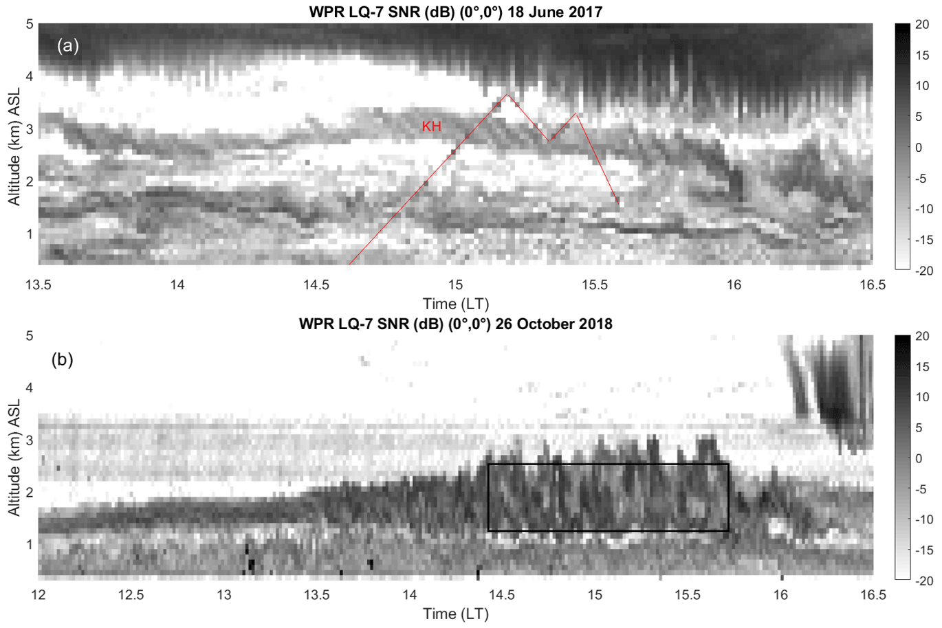
Figure 2Time–height cross-section of WPR LQ-7 SNR (dB) at vertical incidence (0∘, 0∘) (a) on 18 June 2017 from 13:30 to ∼ 16:30 LT (b) on 26 October 2018 from 12:00 to 16:30 LT. Red lines in panel (a) show the track of UAV DataHawk. The black rectangle in panel (b) shows the time–altitude domain selected for analysis.
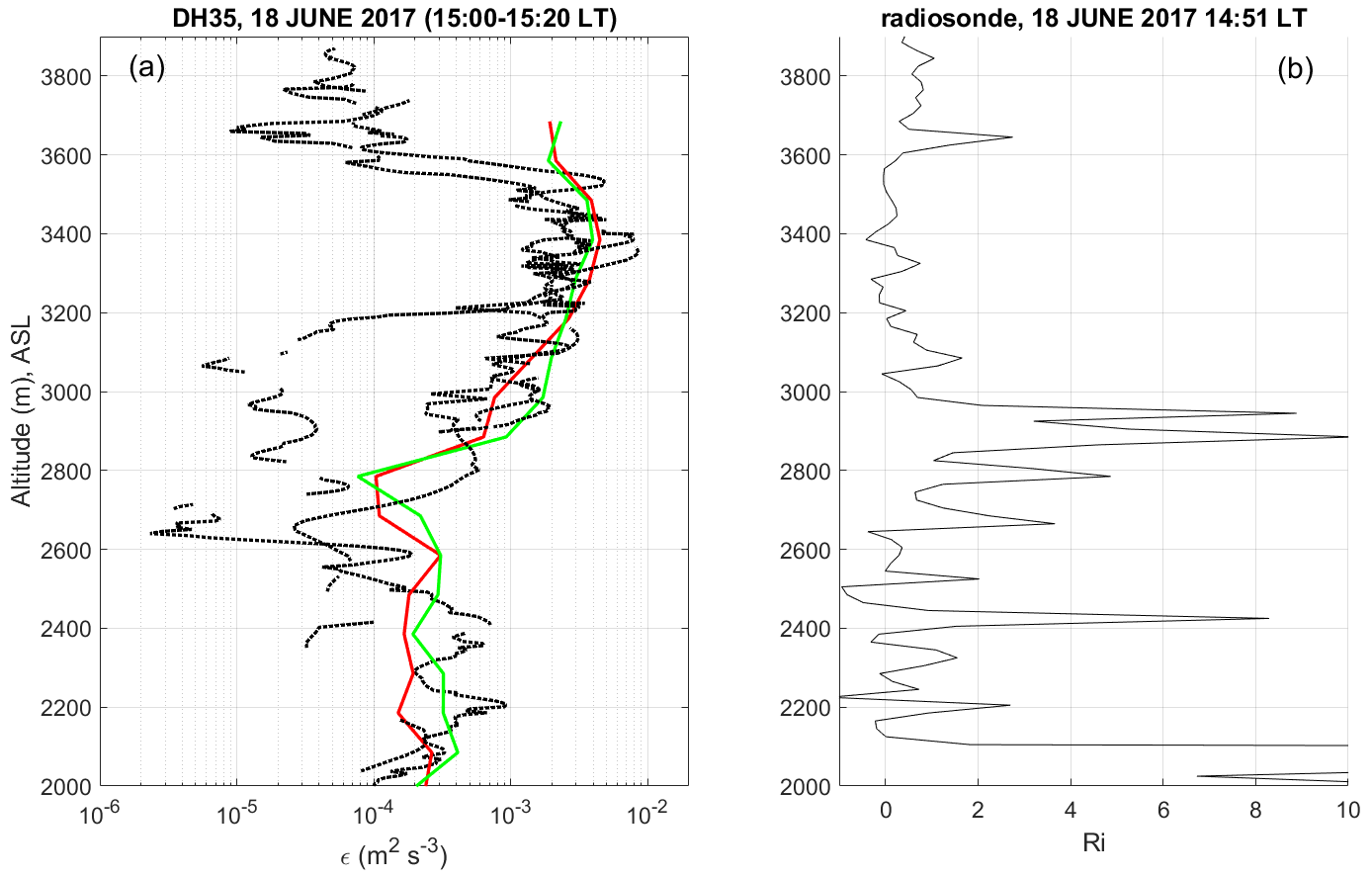
Figure 3(a) DataHawk-derived ε (m2 s−3) profiles in the height range 2000 to 3900 m during the ascents and descents of DataHawk (DH35) on 18 June 2017 (dotted black); εS profile (solid red), εLout profile (solid green) derived from WPR LQ-7 radar data between 15:00 and 15:20 LT. The vertical gray bar indicates the range of the KH layer. (b) Richardson number profile estimated at a vertical resolution of 20 m from a simultaneous radiosonde (called V6). Figure adapted from L2023.
The equivalence between εS and εLout (Fig. 3), i.e.,
was obtained with Lout≈70 m, which had been found to be the canonical value of Lout from the statistical comparison with 90 DataHawk-derived ε profiles (Fig. 4 of L2023). This is likely a coincidence since Lout cannot be treated as a constant. However, if Lout is imposed to be constant, then we obtain σ∼S, which is consistent with the fact that only the shear acts to generate TKE in a neutrally stratified flow. For neutral turbulence, in particular in boundary layers, turbulence length scales are proportional to the depth of the layer (e.g., Zilitinkevich et al., 2019). Therefore, it is expected that Lout is related to the KH layer depth for weak stratification.
KH layers were first visually identified from 59 s resolution time–height cross-sections of SNR (dB) from 0.3 to 5.0 km. Eleven years of data (2011–2021) were screened in 12 h segments. Structures similar to those observed in Fig. 2a were selected, sometimes with the help of the corresponding vertical velocities for confirmation, since KH billows are generally associated with vertical wind disturbances of periods/wavelengths identical to KH billows (e.g., Klostermeyer and Rüster, 1981; Fukao et al., 2011, and references therein). Importantly, the selection criteria do not include wind shear and Doppler spectral width, since they are part of the parameters to be analyzed.
The rejected turbulent layers were as follows:
- a.
all cases that could be confused with convective instabilities at the top of the planetary boundary layer and at the edge of clouds or in precipitating clouds (generally associated with “smooth” echoes),
- b.
all periods during which rain echoes were observed,
- c.
complex structures showing splitting or merging of echo layers or sporadic appearance (extremely frequent),
- d.
layers for which the depth was difficult to identify due to adjacent layers of enhanced echoes and
- e.
layers or parts of layers showing a rapid change in depth or in altitude (because these are difficult to select with the method described below).
The 10 min averaged values of spectral width and winds were selected using a MATLAB program allowing a manual selection of the layer with the mouse in a rectangle of dimensions representative of the duration and depth of the layer, when altitude and depth were nearly constant and echo power did not change significantly. The depth of the KH layer was defined as the average of the maximum and minimum depths of the KH braids, also selected manually. The same KH event, long lasting but slowly moving in altitude and showing temporary fading, may have been selected several times.
Our analysis cannot be considered a statistical study of the occurrence of KH instabilities in the lower troposphere because many of them may have been overlooked unintentionally due to the absence of clearly visible KH braids at the evolution stage of the layer or due to insufficient time and/or range resolution. In particular, their occurrence seems to decrease quickly with height (not shown) because the SNR decreases (blurring effect) and because the wind speed increases (under-sampling effect).
Figure 2b shows one of the deepest KH layers (∼1500 m on average between 14:30 and 15:45 LT) among those selected from the 11 years of data. The portion selected for the analysis is shown by the black rectangle. This event is not representative and shows unusual complex structures that may result from the successive development of several KH instabilities of different scales.
5.1 Analyses of KH layers
Figure 4 shows the histogram of the depth D of the selected KH layers. The mean value is ∼600 m and D exceeds 300 m for 96 % of the layers. Thinner KH layers are difficult or even impossible to identify due to range resolution limitation (100 m). The KH layer described in Sect. 3.2 (∼800 m in depth) is in the upper part of the distribution. Eighty percent of the cases have a selected duration between 30 and 270 min (which is not the total duration of the event).
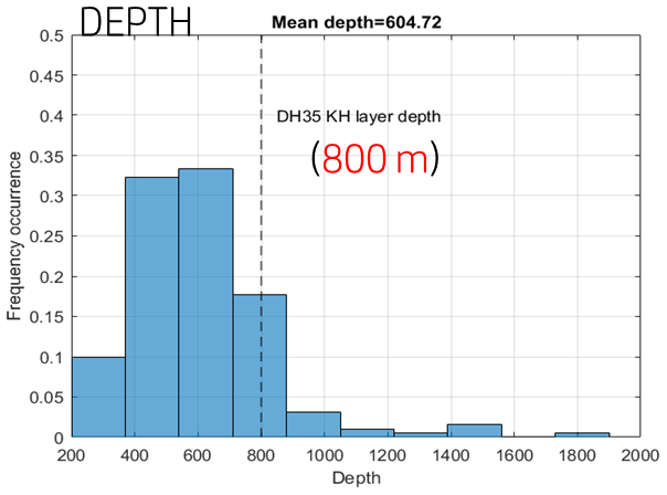
Figure 4Histogram of the depth of the 192 selected KH layers. The depth of the KH layer detected by DH35 (800 m) shown in Fig. 2a is indicated by the vertical dashed line.
Figure 5 shows the scatter plot of log 10(0.64S) vs. using all data for each case. For example, a layer selected between 10:00 and 10:20 LT and between 1000 and 1500 m will contribute to a maximum of values if σ and S are defined everywhere in the rectangle. Figure 6a shows the same information after taking the median (or without substantial differences, the mean) value of all the estimates of σ and S in the time and height of the selected rectangles.
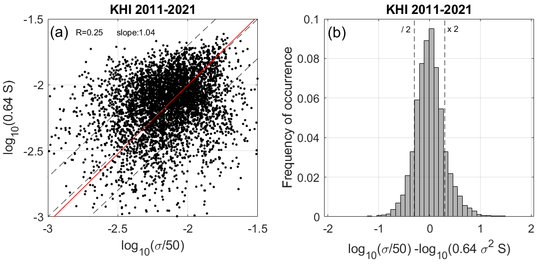
Figure 5(a) Scatter plot of log 10(0.64S) vs. with Lout=50 m for all KH layers at time and height resolutions of 10 min and 100 m, respectively. R is the correlation coefficient. The regression line is shown in red. The slope is given in the insert. (b) Histogram of the difference between log 10(0.63S) and .
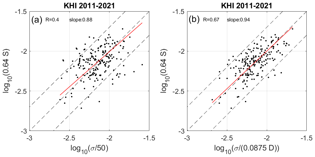
Figure 6(a) Same as in Fig. 5 after averaging all the values of σ and S in time and height domain of the selected rectangles. (b) Same as panel (a) with Lout=0.0875D.
The best agreement in mean level between the two parameters was obtained for 〈Lout〉=50 m in both cases, i.e., slightly less than the canonical value (70 m). In Fig. 5, the dispersion of the distribution is large, but 74 % of the disagreements are less than a factor of 2 for a dynamic of values over 1 decade. The correlation coefficient is 0.25 only but significant according to the P value (=0) and the regression slope is In Fig. 6a, the dispersion is less important (87 % of the disagreements are within a factor of 2). The correlation coefficient increases to 0.41, while the regression slope decreases (0.88). Therefore, Fig. 6a reveals a basic trend between σ and S, less obvious at shorter time and range resolutions, likely because of multiple sources of uncertainties rather than due to a flaw in the assumption.
The influence of the layer depth can be shown in the following way: the ratio is close to , suggesting that Lout is proportional to the depth of the KH layer, i.e., Lout≈0.0875D. Figure 6b shows the scatter plot of log 10(0.64S) vs. . The correlation coefficient significantly increases to 0.67 and the regression slope is 0.94. Ninety-six percent of the disagreements are now within a factor of 2. This is very consistent with the fact that Lout should depend on the depth of the layer for low Ri values. Figure 7a (7b) shows the concatenated values of log 10(0.64S) (red line) and () (black line). The interdependence between the three parameters (σ, S, D) is clear, in particular for the KH events 110 to 140. Then, we obtain
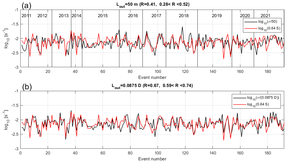
Figure 7(a) Time series of median values of log 10(0.64S) (red line) and (black line) for the 192 KH layers. (b) Same as panel (a) for Lout=0.0875D. R is the correlation coefficient with its lower and upper bounds for a 95 % confidence interval.
In Table 4 of L2023, for the KH layer was found to be 42 m for D=800 m, fully consistent with the above equation, since εS and εLout were found to be equivalent. Figure 8 shows the linear relationship between LH or equivalently Lout and D and an estimate of the slope from a linear regression for all data and for D<1000 m, because very few layers have D>1000 m.
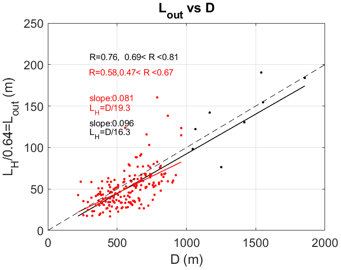
Figure 8Scatter plot of vs. D. Regression lines and slopes are given for all the data (black) and for D<1000 m (red).
Figure 9 shows the scatter plot of log 10(εS) vs. log 10(εLout) for Lout=50 m (left panel) and Lout≈0.0875D (right panel). Due to multiplication by σ2, a strong self-correlation is introduced. The purpose of the figure is to show that, in practice, the equivalence of the two models for KH layers would likely not produce different statistical results if compared with in situ (e.g., DataHawk) measurements.
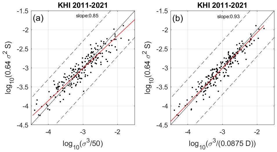
Figure 9(a) Scatter plot of log 10(εS) vs. log 10(εLout) with Lout=50 m. (b) Scatter plot of log 10(εS) vs. log 10(εLout) with Lout=0.0875D.
5.2 Application to other layers
Figures 10–12 show the same information as Figs. 4, 6 and 7 for arbitrarily selected layers using the same method and rejection criteria as described in Sect. 5.1. The only difference is that they do not show evidence of KH braids, because the layers were observed after the total collapse of the KH billows, because they were generated by a different process or because the KH billows were totally blurred by the insufficient time and range resolutions. The objective is to determine to what extent the results obtained for KH layers are also valid for unspecified layers. An arbitrary number of 113 layers was selected from 2017 data.
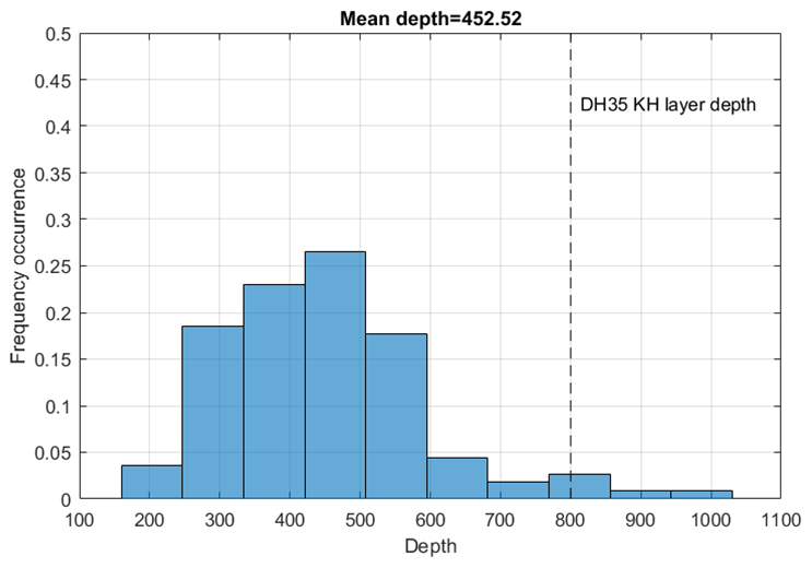
Figure 10Histogram of the depth of the 52 arbitrarily selected layers. The depth of the KH layer detected by DH35 (800 m) shown in Fig. 2a is indicated by the vertical dashed line.
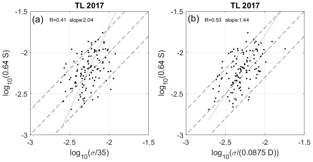
Figure 11(a) Same as in Fig. 6a for 113 arbitrarily selected layers in 2017 with Lout=35 m. (b) Same as panel (a) with Lout=0.0875D.
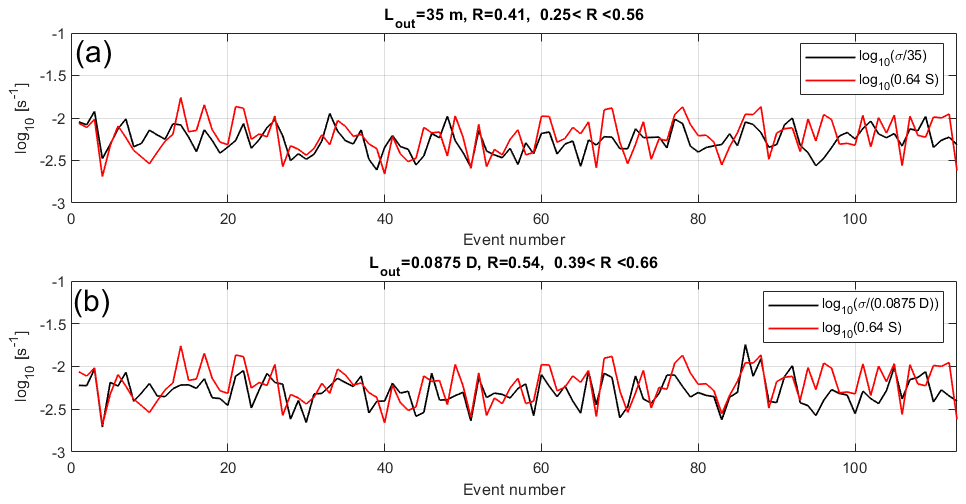
The selected layers are on average thinner: ∼450 m (Fig. 10). The best agreement on average between log 10(0.64S) and was obtained for Lout≈35 m (Fig. 11a), in full accordance with Lout≈0.0875D. The decrease in the dispersion with Lout≈0.0875D (Fig. 11b) is not as important as in Fig. 7b, and the regression slope does not produce a satisfactory trend. The correlation coefficient is lower but increases from 0.4 to 0.53 (Fig. 12). Part of the degradation of the results with respect to KH layers can be due to the increase in the difficulty of defining the layer depth with accuracy, especially for the thinnest ones. But it could also be due to the fact that the hypothesis of equivalence between εS and εLout can sometimes be faulty if Ri is not low. In L2023, the equivalence was not verified for a layer with Ri∼1.
Because the results are mixed, their quality can be considered fair if the objective is to obtain rough estimates of dissipation rates for climatological studies and likely insufficient if precise estimates are necessary.
It was verified that comparisons between σ and S for layers associated with rain echoes and convection (for example) in clouds do not reveal (not shown) similar trends and significant correlations. Therefore the results described for KH layers correspond to physical properties of turbulence.
The present analyses, along with those described in L2023, suggest that the canonical value of Lout (∼70 m) of the empirical model εLout that fits in situ measurements of TKE dissipation rates from DataHawk UAVs is not related to instrumental effects (i.e., to the dimensions of the radar resolution volume) but to a typical depth (∼600 m) of the detected turbulent layers. This interpretation is valid for KH layers at least. This is an important finding because it means that εLout with Lout∼70 m can be applied to any Doppler VHF or UHF radar as long as σ2 can be assimilated to the variance of the vertical wind fluctuations produced by turbulence. In particular, this property likely explains why εLout works for both the MU radar (Luce et al., 2018) and WPR-LQ7 (L2023). The radar resolution volumes are similar for both instruments at low altitudes, but this is not the reason for the quantitative agreement. Because Lout=0.0875D, the radar range resolution Δr is a limiting factor as D must be significantly greater than Δr to be estimated. In this regard, the canonical value of Lout would likely be much less than 70 m if Δr≪100, 150 m because layers much thinner than ∼600 m would be included.
In addition, the estimation of the depth can be difficult in practice when there are multiple and adjacent layers or not well-defined structures. The equivalent model, εS, is more easily applicable. The main criterion for the validity of εS (or εLout with Lout=0.0875D) is low Ri. Therefore, wherever this condition is met, εS should be valid, even for stratospheric turbulence, where the background stratification is typically about 4 times more stable. Many observations suggest the existence of anisotropic turbulence in a stable stratified environment such as the stratosphere. It is also one of the most widespread hypotheses used to explain the angular dependence of VHF radar echoes (Hocking, 1986). This anisotropy can only be explained by the influence of the stable stratification which inhibits the vertical component of turbulence (when Ri is large). Therefore, the εS model may not be valid in such circumstances.
In the present work, we checked the relevance of a radar model εS of TKE dissipation rate expected to be applicable for weakly stratified or strongly sheared layers. This model predicts a σ2S dependence for low Ri values, while the commonly used model εN for stably stratified conditions predicts a σ2N dependence. The latter was derived from multiple assumptions on the properties of the buoyancy subrange (e.g., Hocking et al., 2016) but without explicit assumptions on Ri. The derivations by Basu and Holtslag (2021) showed that both models are nearly quantitatively equivalent for Ri∼1 only, despite the fact that the two models are based on very different assumptions (see L2023 for more details). Because intense turbulence is expected to be observed for low Ri values, the εN model should underestimate the TKE dissipation rate under these circumstances, a result consistent with the comparisons made with in situ measurements by Luce et al. (2018) and L2023. Applied to turbulence generated by KH instabilities, the εS model was found to be consistent with the εLout model predicting a σ3 dependence but to a first approximation only. The consistency was found to be greater with a model predicting a dependence, compatible with basic models of turbulence in nearly neutral boundary layers. This result suggests that similar dynamics occur in KH layers. As a corollary, the Hunt scale defined as is a more appropriate scale than the buoyancy scale to define the typical turbulence length scale in the observed KH layers because Ri values are low. We found LH≈0.056D. The statistics compiled by L2023 show that εS cannot be used as the model by default as the condition of validity of the model (low Ri values) is not verified in the whole column of the atmosphere. In particular, further studies are needed to check the relevance of the models in the stratosphere with VHF radars.
The eddy coefficient for heat or eddy diffusivity is given by (e.g., Lilly et al., 1974)
where is the mixing coefficient defined as the ratio between the dissipation rates of potential and kinetic energies. Using , we obtain the standard equation
where C=CNγ is ∼0.16 if CN∼0.5 and Rf=0.25 as often arbitrarily assumed in the literature (e.g., Lilly et al., 1974; Fukao et al., 1994; Kurosaki et al., 1996; Naström and Eaton, 1997). Note that the arbitrary choice of Rf is made to avoid an inconsistency, when Rf and N approach 0, under neutral stratification. This inconsistency is removed when using Eq. (2), valid for low Ri values. Indeed, when introduced in Eq. (A1), we obtain
which becomes
when Rf approaches 0 since the turbulent Prandtl number Pr goes to 0.8 for low Ri values. Note that 0.8 is a true constant as long as the stationarity assumption remains true, unlike C in Eq. (A2). Equation (A4) is thus an alternative equation for Eq. (A2) for weakly stratified/strongly sheared conditions. Like εS (Eq. 2), Eq. (A4) is independent of N and can be readily estimated from radar measurements of 〈w′2〉 and S. Equations (A4) and (A2) are quantitatively identical when Ri≈0.04 and Eq. (A2) leads to KH values ∼2.5 times smaller than Eq. (A4) when Ri≈0.25.
The WPR-LQ-7 data are available on http://www.rish.kyoto-u.ac.jp/radar-group/blr/shigaraki/data/ (RISH, 2023).
HL wrote the paper with the help of LK and HH.
The contact author has declared that none of the authors has any competing interests.
Publisher's note: Copernicus Publications remains neutral with regard to jurisdictional claims made in the text, published maps, institutional affiliations, or any other geographical representation in this paper. While Copernicus Publications makes every effort to include appropriate place names, the final responsibility lies with the authors.
This study was partially supported by JSPS KAKENHI grant no. JP15K13568 and the research grant for Mission Research on Sustainable Humanosphere from Research Institute for Sustainable Humanosphere (RISH), Kyoto University. Lakshmi Kantha received partial support from the US Office of Naval Research (ONR) MISO/BoB DRI under grant no. N00014-17-1-2716.
This paper was edited by Yuanjian Yang and reviewed by two anonymous referees.
Balsley, B. B., Svensson, G., and Tjernström, M.: On the Scale-dependence of the Gradient Richardson Number in the Residual Layer, Bound.-Lay. Meteorol., 127, 57–72, https://doi.org/10.1007/s10546-007-9251-0, 2008.
Basu, S. and Holtslag, A. A. M.: Turbulent Prandtl number and characteristic length scales in stably stratified floaws: steady-state analytical solutions, Environ. Fluid Mech., 21, 1273–1302, https://doi.org/10.1007/s10652-021-09820-7, 2021.
Basu, S. and Holtslag, A. A. M.: Revisiting and revising Tatarskii’s formulation for the temperature structure parameter C in atmospheric flows, Environ. Fluid Mech., 22, 1107–1119, https://doi.org/10.1007/s10652-022-09880-3, 2022.
Basu, S., He, P., and De Marco, A. W.: Parameterizing the energy dissipation rate in stably stratified flows, Bound.-Lay. Meteorol., 178, 167–184, https://doi.org/10.1007/s10546-020-00559-0, 2021.
Doviak, R. J. and Zrnić, D. S.: Doppler radar and weather observations, Academic Press, San Diego, ISBN 012221420X, 9780122214202, 1984.
Fukao, S., Yamanaka, M. D., Ao, N., Hocking, W. K., Sato, T., Yamamoto, M., Nakamura, T., Tsuda, T., and Kato, S.: Sea-sonal variability of vertical eddy diffusivity in the middle at- 80 mosphere, 1. Three-year observations by the middle and upper atmosphere radar, J. Geophys. Res.-Atmos., 99, 18973–18987, https://doi.org/10.1029/94JD00911, 1994
Fukao, S., Luce, H., Mega, T., and Yamamoto, M. K., Extensive studies of large-amplitude Kelvin–Helmholtz billows in the lower atmosphere with VHF middle and upper atmosphere radar, Q. J. Roy. Meteor. Soc., 137, 1019–1041, https://doi.org/10.1002/qj.807, 2011.
Hocking, W. K.: On the extraction of atmospheric turbulence parameters from radar backscatter Doppler spectra. I. Theory, J. Atmos. Terr. Phys., 45, 89–102, https://doi.org/10.1016/S0021-9169(83)80013-0, 1983.
Hocking, W. K.: Observations and measurements of turbulence in the middle atmosphere with a VHF radar, J. Atmos. Terr. Phys., 48, 655–670, https://doi.org/10.1016/0021-9169(86)90015-2, 1986.
Hocking, W. K., Röttger, J., Palmer, R. D., Sato, T., and Chilson, P. B.: Atmospheric radar, Cambridge University Press, ISBN 9781107147461, 2016.
Hunt, J. C. R., Stretch, D. D., and Britter, R. E.: Length scales in stably stratified turbulent flows and their use in turbulence models, in: Stably stratified flow and dense gas dispersion, edited by: Puttock, J. S., Clarendon Press, Oxford, 285–321, 1988.
Imai, K., Nakagawa, T., and Hashiguchi, H.: Development of tropospheric wind profiler radar with Luneberg lens antenna (WPR LQ-7), Electric Wire & Cable, Energy, 64, 38–42, 2007.
Kantha, L., Lawrence, D., Luce, H., Hashiguchi, H., Tsuda, T., Wilson, R., Mixa, T., and Yabuki, M.: Shigaraki UAV-Radar Experiment (ShUREX 2015): An overview of the campaign with some preliminary results, Prog. Earth and Planet. Sci., 4, 19, https://doi.org/10.1186/s40645-017-0133-x, 2017.
Klostermeyer, J. and Rüster, R.: Further study of a jet stream-generated Kelvin-Helmholtz instability, J. Geophys. Res., 86, 6631–6637, https://doi.org/10.1029/JC086iC07p06631, 1981.
Kurosaki, S., Yamanaka, M. D., Hashiguchi, H., Sato, T., and Fukao, S.: Vertical eddy diffusivity in the lower and middle atmosphere: a climatology based on the MU radar observations during 1986–1992, J. Atmos. Sol.-Terr. Phy., 58, 727–734, https://doi.org/10.1016/0021-9169(95)00070-4, 1996.
Lawrence, D. A. and Balsley, B. B.: High-Resolution Atmospheric Sensing of Multiple Atmospheric Variables Using the DataHawk Small Airborne Measurement System, J. Atmos. Ocean. Tech., 30, 2352–2366, https://doi.org/10.1175/JTECH-D-12-00089.1, 2013.
Lilly, D. K., Waco, D. E., and Adelfang, S. I.: Stratospheric mixing estimated from high-altitude turbulence measurements, J. Appl. Met. Clim., 13, 488–493, https://doi.org/10.1175/1520-0450(1974)013<0488:SMEFHA>2.0.CO;2, 1974.
Luce, H., Hassenpflug, G., Yamamoto, M., and Fukao, S.: Comparisons of refractive index gradient and stability profiles measured by balloons and the MU radar at a high vertical resolution in the lower stratosphere, Ann. Geophys., 25, 47–57, https://doi.org/10.5194/angeo-25-47-2007, 2007.
Luce, H., Kantha, L., Hashiguchi, H., Lawrence, D., and Doddi A.: Turbulence Kinetic Energy Dissipation Rates Estimated from Concurrent UAV and MU Radar Measurements, Earth Planets Space, 70, 207, https://doi.org/10.1186/s40623-018-0979-1, 2018.
Luce, H., Kantha, L., Hashiguchi, H., Lawrence, D., Doddi, A., Mixa, T., and Yabuki, M.: Turbulence kinetic energy dissipation rate: assessment of radar models from comparisons between 1.3 GHz wind profiler radar (WPR) and DataHawk UAV measurements, Atmos. Meas. Tech., 16, 3561–3580, https://doi.org/10.5194/amt-16-3561-2023, 2023.
Naström, G. D. and Eaton, F. D.: Turbulence eddy dissipation rates from radar observations at 5–20 km at White Sands Missile Range, New Mexico, J. Geophys. Res.-Atmos., 102, 19495–100 19505, https://doi.org/10.1029/97JD01262, 1997.
RISH: Boundary Layer Radar (BLR)/Lower Troposphere Radar (LTR)/LQ7 Observation Data, RISH (Research Institute for Sustainable Humanosphere) [data set], Version 02.0212, http://www.rish.kyoto-u.ac.jp/radar-group/blr/shigaraki/data/ (last access: 28 October 2023), 2023.
Schumann, U. and Gerz, T.: Turbulent mixing in stably stratified shear flows, J. Appl. Meteorol., 34, 33–48, https://doi.org/10.1175/1520-0450-34.1.33, 1995.
Zilitinkevich, S., Druzhinin, O., Glazunov, A., Kadantsev, E., Mortikov, E., Repina, I., and Troitskaya, Y.: Dissipation rate of turbulent kinetic energy in stably stratified sheared flows, Atmos. Chem. Phys., 19, 2489–2496, https://doi.org/10.5194/acp-19-2489-2019, 2019.
- Abstract
- Introduction
- The WPR-LQ-7
- The εS model and its application to a case study
- Method and criteria used for KH layer selection
- Statistical analyses
- Discussions
- Conclusions
- Appendix A: Derivation of the equation for heat diffusivity at low Ri values
- Data availability
- Author contributions
- Competing interests
- Disclaimer
- Financial support
- Review statement
- References