A neural-network-based method for generating synthetic 1.6 µm near-infrared satellite images

In combination with observations from visible satellite channels, near-infrared channels can provide valuable additional cloud information, e.g. on cloud phase and particle sizes, which is also complementary to the information content of thermal infrared channels. Exploiting near-infrared channels for operational data assimilation and model evaluation requires a sufficiently fast and accurate forward operator. This study presents an extension to the method for fast satellite image synthesis (MFASIS) that allows for simulating reflectances of the 1.6 µm near-infrared channel based on a computationally efficient neural network with the same accuracy that has already been achieved for visible channels. For this purpose, it is important to better represent vertical variations in effective cloud particle radii, as well as mixed-phase clouds and molecular absorption in the idealized profiles used to train the neural network. A new approach employing a two-layer model of water, ice and mixed-phase clouds is described, and the relative importance of the different input parameters characterizing the idealized profiles is analysed. A comprehensive data set sampled from Integrated Forecasting System (IFS) forecasts together with different parameterizations of the effective water and ice particle radii is used for the development and evaluation of the method. Further evaluation uses a month of ICOsahedral Non-hydrostatic development based on version 2.6.1 (ICON-D2) hindcasts with effective radii directly determined by the two-moment microphysics scheme of the model. In all cases, the mean absolute reflectance error achieved is about 0.01 or smaller, which is an order of magnitude smaller than typical differences between reflectance observations and corresponding model values. The errors related to the imperfect training of the neural networks present only a small contribution to the total error, and evaluating the networks takes less than a microsecond per column on standard CPUs. The method is also applicable for many other visible and near-infrared channels with weak water vapour sensitivity.

1 Introduction

Over the last decades, satellite observations have become the most important observation type assimilated in numerical weather prediction (NWP) systems. They dominate not only in terms of the total number of assimilated observations, but also with respect to the overall impact on the forecast quality of operational global NWP systems (Bormann et al., 2019; Eyre et al., 2022). The preferred way to assimilate satellite observations from imagers and sounders is the direct assimilation of radiances, which requires a forward operator to generate synthetic radiances from the NWP model state. In contrast to assimilating retrievals, no external a priori information (e.g. from other models or climatologies) is required in the direct assimilation approach, and in general the characterization of errors is also less problematic (Errico et al., 2007). Satellite radiances are increasingly assimilated not only in clear-sky conditions, but also in the presence of clouds and precipitation. This so-called “all-sky” approach is being applied successfully to microwave (MW) observations in different global NWP systems (Geer et al., 2018), and progress is being made towards the direct all-sky assimilation of infrared (IR) observations (Geer et al., 2018, 2019; Li et al., 2022). Similarly, satellite observations are also assimilated in many regional models (Gustafsson et al., 2018) with a particular focus on observations from geostationary imagers providing temperature, moisture and cloud information with high temporal and spatial resolution (see e.g. Otkin and Potthast, 2019; Okamoto, 2017).

Efforts to improve the exploitation of satellite observations that are currently underutilized are ongoing, both in terms of assimilating already operational data under all conditions and over all surfaces and in terms of using channels that are not yet directly assimilated at all (Valmassoi et al., 2022; Hu et al., 2022). Solar satellite channels fall into the latter category, mostly because sufficiently fast and accurate forward operators are missing or have only become available recently. The development of such operators was hampered by the fact that standard radiative transfer (RT) methods for the solar spectral range (with wavelengths λ<4 µm) are computationally very expensive, as they require the detailed modelling of multiple scattering processes, which are much more important than in the thermal part of the spectrum (λ>4 µm). Moreover, 3D RT effects, i.e. effects involving horizontal photon transport, e.g. related to inclined cloud tops, cloud shadows or complex topography (see Marshak and Davis, 2005, for a detailed discussion), can be important for solar channels, especially at high resolutions and for large zenith angles. For visible channels Scheck et al. (2016) developed a method for fast satellite image synthesis (MFASIS), an efficient 1D RT approach based on a strong simplification of the vertical cloud structure and the use of precomputed results stored in compressed lookup tables (LUTs). This LUT-based version of MFASIS has been integrated into the Radiative Transfer for TOVS (RTTOV) satellite forward operator package in v12.2 with subsequent improvements in v12.3 and v13.1 (Saunders et al., 2018, 2020). MFASIS has been used in several model evaluation studies (Heinze et al., 2016; Stevens et al., 2020; Sakradzija et al., 2020; Geiss et al., 2021) as well as data assimilation studies (Schröttle et al., 2020; Scheck et al., 2020). The assimilation of visible SEVIRI (Spinning Enhanced Visible and InfraRed Imager) observations at 0.6 µm using RTTOV-MFASIS became operational at DWD (Deutscher Wetterdienst, German Meteorological Service) in March 2023. An extension to MFASIS to account for the most important 3D RT effects in a computationally efficient way is available (Scheck et al., 2018), and recently a faster and more flexible version based on neural networks instead of LUTs has been developed (Scheck, 2021a) and integrated into RTTOV 13.2.

The cloud information contained in visible channels is complementary to that available from thermal infrared channels. While visible channels provide almost no information that could be used to determine the cloud top height or discriminate frozen clouds from liquid clouds, they contain much more information on the cloud water or cloud ice content as they saturate only for much thicker clouds than thermal channels (Geiss et al., 2021). There is also some dependency of visible radiances on the cloud particle sizes and the surface structure of clouds.

Near-infrared (NIR) channels ($\mathrm{0.75}\le \mathit{\lambda }\le \mathrm{4}$ µm) depend on cloud particle sizes and angles in a different way, compared to visible channels, and can thus provide additional information that could be very valuable for both model evaluation and data assimilation. The combined information of visible and near-infrared channels has been successfully used for many years to simultaneously retrieve cloud optical thickness and effective particle radii (following Nakajima and King, 1990). Such observations constraining the cloud microphysics are also of special relevance for NWP models employing advanced cloud physics schemes like two-moment schemes that provide prognostic effective cloud particle sizes (see e.g. Seifert and Beheng, 2006). Of particular interest is the 1.6 µm channel available on many satellite imagers because at this wavelength ice absorbs radiation considerably stronger than water. In combination with a visible channel, for which absorption by both water and ice is very weak, the 1.6 µm channel can thus provide information that is helpful for distinguishing liquid clouds from frozen clouds (but will not in all cases allow for a clear distinction; see e.g. Fig. 4 in Coopman et al., 2019). While information on the cloud phase is also available from thermal infrared channels, using near-infrared channels in addition (Baum et al., 2000) or instead (Nagao and Suzuki, 2021) can improve the reliability of retrievals. Assimilating the 1.6 µm channel could thus be a promising way to reduce cloud-phase errors.

MFASIS can already be applied to NIR channels, and LUTs for 1.6 µm channels of different instruments are available as part of the RTTOV package. However, mainly due to the rather approximate treatment of mixed-phase clouds, the currently employed method is considerably less accurate for this channel. Some corrections included in RTTOV 13.1 allow for avoiding the largest errors, but the accuracy in the 1.6 µm channel is still lower than in visible channels. This study demonstrates how to both improve the accuracy and reduce the computational effort through using a machine-learning-based approach. We focus on generating synthetic images for the 1.6 µm channel of the SEVIRI instrument aboard Meteosat Second Generation (MSG) from global and regional NWP model data. Building on the neural-network-based results for visible channels of Scheck (2021a), suitable network input parameters to account for the more complex dependency of near-infrared radiances on the atmospheric state will be identified. Networks with these input parameters are then trained and tested on different data sets.

The rest of this study is organized as follows: data and methods are discussed in Sect. 2, suitable network input parameters are derived in Sect. 3, the training of neural networks based on these profiles is discussed in Sect. 4, the full method is evaluated using different data sets in Sect. 5 (also for other solar channels) and conclusions are given in Sect. 6.

2 Data and methods

2.1 Radiative transfer methods

2.1.1 DOM

For reference calculations and the generation of neural network training data, the discrete ordinate method (DOM; see Stamnes et al., 1988) is used. We rely on the implementation of DOM in the RTTOV package (Saunders et al., 2018). The required input data comprise vertical profiles of the cloud water and cloud ice content, including the corresponding effective particle radii, a value for the surface albedo (A), solar and satellite zenith angles (θ₀, θ), and the difference in their azimuth angles (Δϕ). DOM solves the plane-parallel radiative transfer equations and computes the resulting top-of-atmosphere reflectance. In RTTOV, the liquid cloud optical properties used in this process are based on Mie (1908), and for ice clouds the optical properties for the general habit mixture of Baum et al. (2005, 2007) are used. Aerosols are neglected in this study, but clear-sky Rayleigh scattering and molecular absorption are taken into account.

2.1.2 MFASIS

DOM generates accurate 1D RT solutions but is significantly too slow for operational applications like data assimilation. For this reason, the fast method MFASIS (Scheck et al., 2016) was developed and has subsequently been implemented in RTTOV (beginning with version 12.2; see Saunders et al., 2020). In MFASIS, the cloud top height and details of the vertical cloud structure are not taken into account for computing the reflectance, and still the reflectance errors with respect to the DOM solution are small. These properties of the input profiles can therefore be considered to be not very important for the resulting reflectance. The complex vertical profiles from NWP runs are in MFASIS replaced by highly idealized profiles with the same total optical depths and mean effective particle radii. These idealized profiles contain a homogeneous ice cloud above a homogeneous water cloud at fixed heights embedded in a standard atmosphere. Only eight parameters are used to fully characterize the idealized radiative transfer problem: the optical depths and vertically averaged effective particle radii for the water and the ice cloud, three angles to define the sun–satellite geometry, and the surface albedo. Reflectances for many combinations of the parameters are precomputed using DOM and are stored in an 8D lookup table (LUT). The latter is reduced from 8 GB to 21 MB using a lossy compression method. To obtain reflectances for arbitrary input profiles, it is only necessary to compute the input parameters from them and interpolate the reflectance in the LUT at the corresponding location.¹ This process only takes several microseconds and is thus orders of magnitude faster than running DOM. Both the achieved speed and the accuracy are sufficient for assimilation of visible radiance observations in operational applications.

While the simplification of the vertical profiles in MFASIS causes reflectance errors that are acceptable for data assimilation or model evaluation using visible channels, they remain significantly larger for the 1.6 µm near-infrared channel that is considered in this study for three reasons:

• The absorption in ice is considerably stronger than in water. Replacing mixed-phase clouds, which are often dominated by liquid water at the top, by an ice cloud above a water cloud therefore causes large errors.

• The 1.6 µm channel is slightly affected by molecular absorption (due to CO₂, CH₂ and for wider channels like the one on the SEVIRI instrument considered here also water vapour), which means that the air mass between the cloud and satellite will have a stronger influence on the reflectance than in visible channels.² For SEVIRI the water vapour mass will also have some influence. To give an example, for a relatively high column-integrated water vapour content of 50 mm and solar and satellite zenith angles of 60^∘ the reflectance is reduced by about 5 %.

• The vertical variation in the effective particle radii is not taken into account in the simplified profiles. While this error source alone would still be acceptable (it is indeed also present for visible channels), it contributes significantly to the total error, in addition to the two other problems listed above. The problem is that the effective radii in the uppermost cloud layers, from which photons can escape after single-scattering events, may be different from the effective radii at higher optical depths that contribute to the reflectance by multiple scattering processes. To approximate both the correct scattering angle dependence of the reflectance, which is dominated by single-scattering processes, and the correct angle-averaged reflectance, which is often dominated by multiple scattering processes, at least two different radii are required.

Preliminary solutions to account for the largest errors were introduced into the MFASIS implementation in RTTOV v13.1: replacing ice within or below water clouds with water clouds of the same optical depth reduced the errors for mixed-phase clouds. The computation of the mean effective radius was modified to give more weight to the upper cloud layers for thick clouds. While these corrections succeeded in removing the largest errors, the mean errors are still considerably larger than in visible channels. In this study we present a new approach, which is more accurate and faster as well as based on neural networks.

2.1.3 Neural networks and MFASIS-NN

Artificial neural networks are the most popular machine learning approach. They have the advantages that mature, easy-to-use implementations are available and that many CPUs and GPUs now support hardware-accelerated training and evaluation of these networks. A neural-network-based version of MFASIS for visible channels, in the following referred to as MFASIS-NN, has been developed by Scheck (2021a). While the simplification of vertical profiles in this method is the same as in MFASIS, the LUT is replaced by a deep feed-forward neural network. The input parameters of the network correspond to the dimensions of the LUT. Reflectances for arbitrary albedo values can be computed from the three output parameters approximating reflectances for surface albedo values 0, 0.5 and 1 (see Eq. 6 in Scheck, 2021a, and the discussion in Sect. 4.1). The study shows that networks with several thousand parameters in four to eight hidden layers can be trained well enough to achieve reflectance errors that are in general smaller than the ones of the LUT version. The amount of data to be generated with DOM for the training is a factor of 1000 smaller than the 8 GB required for the LUT-based MFASIS. Moreover, using a computationally cheap activation function and a Fortran inference code optimized for small networks, MFASIS-NN is an order of magnitude faster than the LUT-based MFASIS.

As in Scheck (2021a), deep feed-forward neural networks are used in this study. Networks with 8 hidden layers and 15, 25 or 32 nodes per layer are considered. The networks are initialized with random numbers and trained with the open-source TensorFlow package (Abadi et al., 2015) using standard methods. The mini-batch gradient descent method (with a batch size of 256) and the Adam algorithm (see Chap. 8 in Goodfellow et al., 2016) with a learning rate of $\mathrm{2.5}\times {\mathrm{10}}^{-\mathrm{4}}$ were utilized for this purpose. About 1.4×10⁷ synthetic training data samples were generated by assuming random numbers for the normalized network input parameters (uniformly distributed in [0,1], which means that the unnormalized, physical variables are uniformly distributed over the ranges given by Table 2) and by computing the corresponding reflectance with DOM. A total of 80 % of the samples were used for the training, and 20 % served as independent validation data. The networks were trained for 4000 epochs. During the training, the updated network weights and biases were stored only if they resulted in a reduced root-mean-square error of the validation data set, an approach known as early stopping. For the evaluation or inference of networks, we employed FORNADO, an optimized Fortran code including tangent linear and adjoint versions. To reduce the computational effort, the “cheap soft unit” (CSU; see Fig. 2 in Scheck, 2021a), defined as

$$\begin{array}{}\text{(1)}& f_{\text{CSU}}\left(x\right)=\left\{\begin{array}{lcl}\mathrm{0},& \text{if}& x<-\mathrm{2}\\ -\mathrm{1}+\mathrm{0.25}(x+\mathrm{2}{)}^{\mathrm{2}},& \text{if}& x\in [-\mathrm{2},\mathrm{0}]\\ x,& \text{if}& x>\mathrm{0},\end{array}\right.\end{array}$$

was used as an activation function for the hidden layers. This function is very similar to the well-known exponential-linear unit (ELU), $f_{\text{ELU}}\left(x\right)=min\left(e^x-\mathrm{1},\left|x\right|\right)$, but does not involve a computationally expensive exponential function, which can also prevent the compiler from using vector instructions. For the output nodes, we used the softplus function, $f_{\text{softplus}}\left(x\right)=\ln (\mathrm{1}+e^x)$, which guarantees that all output values are positive.

2.2 NWP SAF profiles

A comprehensive set of profiles available from the Satellite Application Facility for Numerical Weather Prediction (NWP SAF) project is used to tune and evaluate the methods developed for this study. The data set comprises 5000 individual profiles selected from a year (1 September 2013–31 August 2014) of short-range forecasts produced with the Integrated Forecasting System (IFS) of the European Centre for Medium-Range Weather Forecasts (ECMWF) using an algorithm which only selects profiles that are sufficiently different in cloud variables compared to the other selected profiles. The profiles represent realistic seasonal variability, and, as they are spread over the entire globe, global variability is also well represented. About 30 % of the profiles are located over land and about 40 % between the northern and southern tropics. Refer to Eresmaa and McNally (2014) for further information about the data set. It should be noted that the cloud fraction profiles, c(z), were modified for this study. To avoid having to take cloud overlap into account, for which different assumptions exist (see e.g. Scheck et al., 2018) and which is not the focus of this work, the cloud fraction was set to zero for $c<\frac{\mathrm{1}}{\mathrm{2}}$ and to one for $c\geqq \frac{\mathrm{1}}{\mathrm{2}}$. While this simplification certainly has some impact on the distribution of total optical depths, it should not pose a serious limitation while making reference calculations with DOM much cheaper.³

The NWP SAF profiles do not contain any information on effective cloud particle sizes, which are required for RT calculations. Therefore, parameterizations have to be used. For effective radii of water cloud droplets, the parameterization of Martin et al. (1994) is used, which depends on the liquid water content and a droplet number concentration N_C. Here, we adopt either N_C=100 cm⁻³ or N_C=200 cm⁻³, which are typical values used in NWP models. For effective ice particle sizes we rely either on the parameterization by McFarquhar et al. (2003), which depends only on the ice content, or on the one by Wyser (1998), which depends in addition on the temperature. All of these radius parameterizations can produce unrealistically small radii for low water/ice contents and under certain conditions also radii that are larger than the maximum radii RTTOV accepts. To reduce the impact of these cases, we limit the effective droplet radii to the range [5 µm,25 µm] and the effective ice particle radii to the range [20 µm,60 µm], as in Scheck et al. (2016). With these effective radii and the water/ice contents from the IFS data, extinction coefficient profiles for water and ice cloud layers (β_w(z) and β_i(z)) can be computed using channel-specific conversion factors provided by RTTOV. The vertical integrals of β_w(z) and β_i(z) are the water and ice optical depths τ_w and τ_i. From their distribution (Fig. 1) it is evident that there is a wide variety of water, ice and mixed-phase clouds with optical depths up to several hundreds.

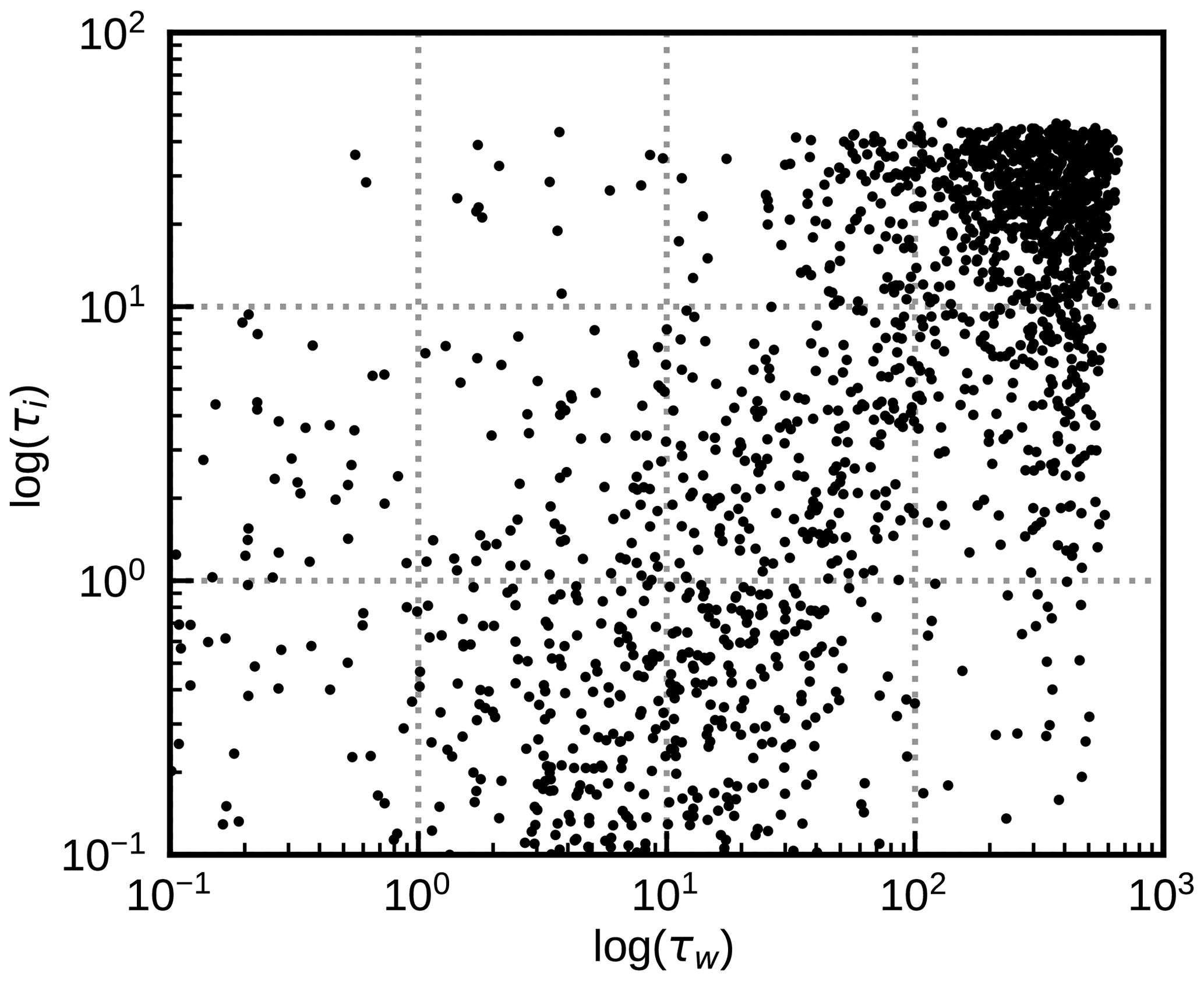
Figure 1 Water cloud optical depth τ_w and ice cloud optical depth τ_i for all profiles of the std data set (see Table 1).

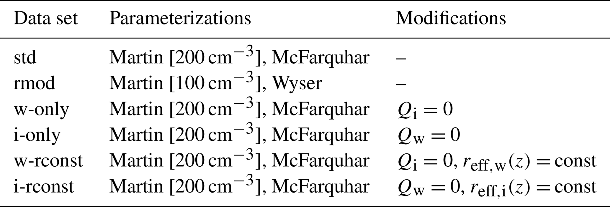
Table 1 Profile data sets used in this study, based on the NWP SAF profiles. In some of the data sets the water or ice cloud mixing ratios, Q_w and Q_i, are set to zero; the effective radii are set to a constant value in each profile (the mean value in the profile); or the radii are computed for a different droplet number concentration (specified in brackets) in the droplet size parameterization by Martin et al. (1994) or using the Wyser (1998) parameterization instead of the McFarquhar et al. (2003) parameterization for ice particles.

In Table 1 the different versions of the profile data set used in this study are listed, which differ in their effective radius parameterizations, the cloud types present in the profiles and the vertical variation in the effective radii. The different parameterizations lead to significantly different mean effective radius distributions, as shown in Fig. 2. A smaller droplet concentration (Fig. 2b) leads to larger droplet radii than for the standard value of N_C=200 cm⁻³ (Fig. 2a). The ice particle radii computed with Wyser (1998) (Fig. 2d) show more spread and depend differently on the optical depth than those computed using McFarquhar et al. (2003) (Fig. 2c). The data sets with only water or only ice clouds allow for investigating these cloud types separately. The data sets in which the effective radius profile is replaced by its mean value in each profile are used to switch off the impact of vertical radius gradients.

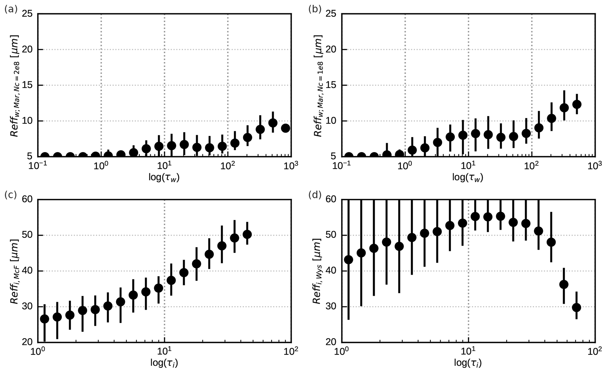
Figure 2 Mean vertically averaged effective particle radii (dots) in logarithmically spaced optical depth bins for the std (a, c) and rmod (b, d) profile data sets for water clouds (a, b) and ice clouds (c, d). The vertical lines connect the 5th and the 95th percentiles for each bin.

To compute top-of-atmosphere reflectances for the profiles in these data sets using DOM, the cloud variables as well as the sun and satellite angles and the surface albedo are required. For all the profiles, longitude, latitude and time are known, so these additional parameters could be determined. However, we follow a different approach, which increases the number of test cases significantly. For each profile, reflectances are computed for 64 angle combinations that are chosen randomly with the constraints $\mathit{\alpha }<\mathrm{130}{}^{\circ }$, $\mathit{\theta }<\mathrm{80}{}^{\circ }$ and ${\mathit{\theta }}_{\mathrm{0}}<\mathrm{80}{}^{\circ }$, where α is the scattering angle with $\mathit{\alpha }=\mathrm{0}{}^{\circ }$ meaning backscattering and $\mathit{\alpha }=\mathrm{180}{}^{\circ }$ forward scattering. Moreover, reflectances are not computed for the surface albedo at the location of the profile, but for each viewing geometry three reflectances are computed for albedo values 0, $\frac{\mathrm{1}}{\mathrm{2}}$ and 1. The three reflectances allow for calculating reflectance for arbitrary albedo values, as discussed in Sect. 3.3 of Scheck (2021a). In total, 5000 × 64 × 3 = 960 000 reflectances are thus computed for each data set and RT method.

Of course the effective radii obtained for the IFS profiles from parameterizations may not be fully realistic. Both features in the vertical profiles and the distribution of mean radii could differ from reality. For this reason, we additionally consider data from a regional model with a two-moment microphysics scheme that generates prognostic information on effective radii, which should be closer to reality (see next section). However, as at least for the next few years most models will be restricted to one-moment microphysics schemes and as this study is aimed at generating synthetic satellite images for these models, it seems appropriate to use effective radii from parameterizations.

2.3 ICON hindcasts

For an additional evaluation of the results we use atmospheric profiles from a 30 d hindcast performed with the convection-permitting, regional ICON-D2 (ICOsahedral Non-hydrostatic, development version based on version 2.6.1; Zängl et al., 2015) model. This NWP model and the resulting profiles are independent and different from the IFS model, which is the basis for the NWP SAF profiles used in the development of the MFASIS near-infrared approach, especially with regard to the cloud microphysics scheme and the resulting effective cloud particle radii. The same ICON-D2 setup as in Geiss et al. (2021) is used, with a domain covering Germany and parts of its neighbouring countries, a horizontal grid spacing of 2.1 km, and 65 vertical levels. The 30 d hindcast is initialized once on 1 June 2020 at 00:00 UTC based on downscaled ICON-EU (Europe nest of global ICON model) analysis initial conditions and uses hourly boundary conditions from ICON-EU analyses.

The test period is characterized by various different summer time weather situations with a wide variety of clouds. As is visible from Fig. 3, most of the clouds are limited to τ_w<100 and τ_i<10. The even thicker clouds present in the IFS profile data sets are probably related to the tropics and are not present in the ICON-D2 domain.

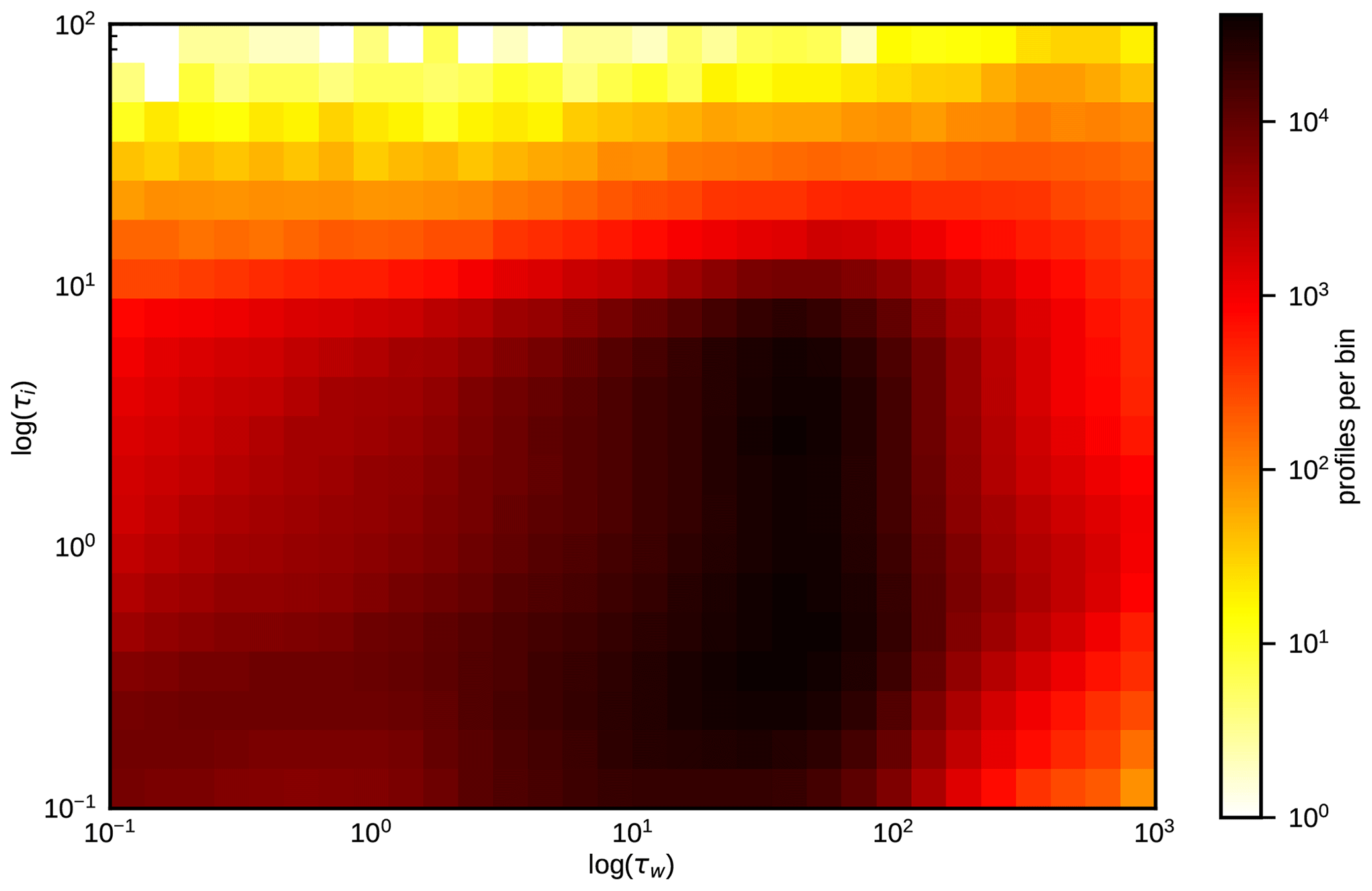
Figure 3 Distribution of water and ice cloud optical depths throughout the domain for all 30 d of the ICON-D2 hindcast period at 12:00 UTC (about 8.3×10⁶ profiles).

An important difference, compared to the IFS-based NWP SAF profiles, is that the ICON-D2 hindcast employs a two-moment microphysics scheme (Seifert and Beheng, 2006). This microphysics scheme directly provides effective radii that should in principle be more realistic than the radii computed with parameterizations. For this reason the lower limit for effective droplet radii applied before running RT calculations is reduced to 2.5 µm for the ICON hindcasts.

The effective radii from the two-moment scheme (Fig. 4) show qualitatively different dependencies on the optical depths compared to those obtained with parameterizations (Fig. 2). For the two-moment calculations the mean effective droplet radius reaches a maximum at τ_w=100 and decreases for higher optical depths, whereas for the parameterization there is a further increase for τ_w>100. The mean effective ice particle radii from the two-moment scheme are more similar to the Wyser results (Fig. 2c) than to the McFarquhar results (Fig. 2d), with radii increasing at smaller optical depths and decreasing at higher optical depths. However, for the two-moment scheme the maximum mean effective radius is already reached at τ_i=4 (not τ_i=30 as for Wyser). Even more obvious differences between parameterized and two-moment radii are found for the spread. The parameterizations mostly depend on quantities strongly correlated with the optical depth, like liquid water content (LWC) and ice water content (IWC), and are therefore quite well-defined functions of the optical depth with a small spread. The only exception is the Wyser parameterization (Fig. 2d), which has an additional dependency on temperature and therefore a larger spread. In contrast, the two-moment radii always show a spread that is considerably larger than for the parameterizations for both water and ice clouds, as is to be expected for more realistic radii.

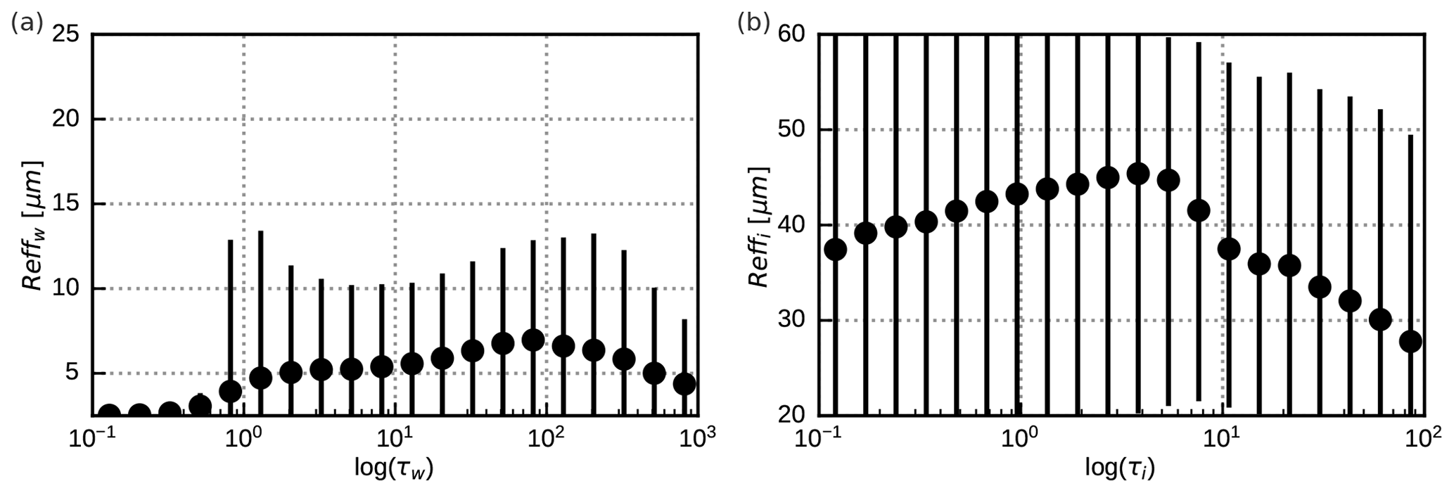
Figure 4 Mean vertically averaged effective particle radii (dots) in logarithmically spaced optical depth bins of the 30 d of the ICON-D2 hindcast period at 12:00 UTC (about 8.3×10⁶ profiles) for water clouds (a) and ice clouds (b). The vertical lines connect the 5th and the 95th percentiles for each bin.

3 Selecting input parameters

3.1 Extending the MFASIS approach

For visible channels it is sufficient to characterize the idealized profiles by only four numbers, optical depths and effective particle radii for a water and an ice cloud at fixed heights. As discussed in Sect. 2.1, these idealized profiles are too simplistic for near-infrared channels. Therefore, additional parameters have to be included to account for the clear-sky absorption, the impact of vertically varying effective radii and the fact that the uppermost part of mixed-phase clouds is often dominated by liquid water.

As a minimal extension to account for vertically varying effective radii, the one-layer ice and water clouds are replaced by two-layer clouds with different effective radii in the upper and the lower layer. Moreover, for a better representation of mixed-phase clouds we allow for the presence of ice in the two-layer water cloud, which can therefore be either a water or a mixed-phase cloud. In contrast, the ice cloud located above this mixed-phase cloud is assumed to be free of liquid water. Thus, in total, six optical depths ${\mathit{\tau }}_C^L$ and six effective particle radii $r_C^L$ have to be specified to fully define the clouds in the idealized profile. Here, $L\in \left[\mathrm{u};\mathrm{l}\right]$ for the upper/lower layers, C=i for the pure ice cloud, C=w for the water content and C=wi for the ice content of the mixed-phase cloud.

When the geometric height at the top, $z_C^{L,\text{top}}$, and the bottom, $z_C^{L,\text{bot}}$, of each layer is known, the optical depths can be computed as

$$\begin{array}{}\text{(2)}& {\mathit{\tau }}_C^L=\underset{z_C^{L,\text{bot}}}{\overset{z_C^{L,\text{top}}}{\int }}{\mathit{\beta }}_C\left(z\right)\mathrm{d}z\end{array}$$

from the profile of the extinction coefficient β_C(z) computed from the NWP model output using the satellite-channel-dependent factors provided by RTTOV (as part of the regression coefficient files). The mean effective particle radii are computed as

$$\begin{array}{}\text{(3)}& r_C^L=\left({\mathit{\tau }}_C^L{)}^{-\mathrm{1}}\underset{z_C^{L,\text{bot}}}{\overset{z_C^{L,\text{top}}}{\int }}{r}_{\text{eff},C}\right(z\left){\mathit{\beta }}_C\right(z)\mathrm{d}z\end{array}$$

from the effective radius profile r_eff,C(z) that is either included in the NWP model output or computed using one of the parameterizations listed in Sect. 2.2. For computing the mixed-phase cloud top height in the NWP profile, we use the cumulative optical depth

$$\begin{array}{}\text{(4)}& {\mathit{\tau }}_C^{\text{cml}}\left(z\right)=\underset{z}{\overset{z_{\text{toa}}}{\int }}{\mathit{\beta }}_C\left(z\right)\mathrm{d}z,\end{array}$$

where z_toa is the height of the uppermost level of the model profile. The mixed-phase cloud top height, $z_{\text{wi}}^{\text{u,top}}$, is then defined to be the height at which ${\mathit{\tau }}_{\mathrm{w}}^{\text{cml}}\left(z\right)$ exceeds a threshold value of 1. To avoid gaps between the integration ranges $z_C^{\text{l,top}}=z_C^{\text{u,bot}}$ and to cover the full profile, we adopt $z_{\mathrm{w}}^{\text{u,top}}=z_{\mathrm{i}}^{\text{u,top}}=z_{\text{toa}}$ and $z_{\mathrm{w}}^{\text{l,bot}}=z_{\text{wi}}^{\text{l,bot}}=z_{\text{sfc}}$, where z_sfc is the height of the lowest level of the model profile.⁴ The only geometric heights that have not been defined so far are those that determine how the two-layer clouds are split in an upper and a lower part, $z_{\mathrm{i}}^{\text{u,bot}}$ and $z_{\mathrm{w}}^{\text{u,bot}}$. A parameterization for the cloud splitting that computes the optical depths of the two parts, ${\mathit{\tau }}_C^{\mathrm{l}}$ and ${\mathit{\tau }}_C^{\mathrm{u}}$, from the total optical depth of the cloud, ${\mathit{\tau }}_C={\mathit{\tau }}_C^{\mathrm{l}}+{\mathit{\tau }}_C^{\mathrm{u}}$, is discussed in Sect. 3.3. Based on these optical depths, $z_{\mathrm{i}}^{\text{u,bot}}$ and $z_{\mathrm{w}}^{\text{u,bot}}$ can be determined.

The impact of clear-sky absorption by the well-mixed trace gases carbon dioxide (CO₂) and methane (CH₄) depends on the air mass above the cloud and, in the case of semi-transparent clouds, also on the air mass above the ground. The latter can be quantified by the cloud top pressure, p_ct, and the surface pressure, p_sfc. Of course, p_ct and p_sfc cannot exactly quantify the clear-sky impact for complex multi-layer cloud situations, but they should still be useful for an approximate description. In this study, the cloud top pressure is defined as the pressure at which the total (water plus ice cloud) optical depth exceeds a threshold value of $min\left(\frac{\mathrm{1}}{\mathrm{2}}{\mathit{\tau }}_{\mathrm{t}},\mathrm{1}\right)$, where τ_t is the column-integrated total optical depth of all water and ice cloud layers. This definition presents a good compromise to prevent on the one hand that very thin, high clouds above thicker clouds trigger the cloud top detection and to avoid on the other hand that the cloud top is detected too deep inside the cloud. Instead of p_ct, we use the dimensionless ratio $f_{\text{ct}}=p_{\text{ct}}/p_{\text{sfc}}$ as input parameter for neural networks. Moreover, absorption by water vapour has some influence on 1.6 µm SEVIRI reflectances, in particular for high albedo values and large zenith angles. Water vapour is not well-mixed, and therefore its impact can not be quantified by just p_ct and p_sfc. As the impact is relatively weak, it is sufficient to use just one parameter to describe the water vapour profile, the vertically integrated water vapour content,

$$\begin{array}{}\text{(5)}& \text{IWV}=\underset{z_{\mathrm{sfc}}}{\overset{z_{\mathrm{toa}}}{\int }}\mathit{\rho }\left(z\right)q_{\mathrm{v}}\left(z\right)\mathrm{d}z,\end{array}$$

where ρ is the density and q_v is the specific humidity. Instead of IWV, we will use the normalized

$$\begin{array}{}\text{(6)}& \text{nIWV}={\displaystyle \frac{(\text{IWV}-{\text{IWV}}_{\min }(p_{\text{sfc}}\left)\right)}{\left({\text{IWV}}_{\max }\left(p_{\text{sfc}}\right)-{\text{IWV}}_{\min }\left(p_{\text{sfc}}\right)\right)}}\end{array}$$

as input parameter for neural networks. This ensures that IWV remains within the range accepted by RTTOV. Details on the fit functions IWV_min and IWV_max can be found in Appendix B.

The definitions that have been provided so far allow for computing the neural network input parameters p_ct, p_sfc, nIWV, ${\mathit{\tau }}_C^L$ and $r_C^L$ from NWP profiles, a step required before reflectances can be computed with the network. For generating the synthetic training data for the network, the inverse step is required: for given network input parameters we need to define full idealized vertical profiles, as the latter are required by DOM to compute the corresponding reflectances. These idealized profiles have to contain the four cloud layers with the desired ${\mathit{\tau }}_C^L$ and $r_C^L$, have the correct IWV, have the correct cloud top pressure p_ct (according to the definition given above), and have to start at the correct surface pressure p_sfc. The geometric thickness of the cloud layers should not be very important for the reflectance. For the sake of simplicity, we modify an IFS standard atmosphere such that one of the pressure levels matches the cloud top pressure and that the surface pressure has the desired value. Then only are the four layers around p_ct filled with ${\mathit{\tau }}_C^L$, $r_C^L$, as shown in Fig. 5, which also illustrates the integration ranges used to compute ${\mathit{\tau }}_C^L$ and $r_C^L$ from an NWP model profile. A standard water vapour profile is scaled such that the correct IWV results. Details on how idealized profiles are computed from the input parameters can be found in Appendix A.

The computation of reflectances for the idealized profiles with two-layer clouds, including a mixed phase, surface and cloud top pressures (as shown in the right half of Fig. 5), and the scaled water vapour background, now requires in total 16 parameters. This assumes that the transmittances of the upper and lower water and ice cloud layers can be computed as a function of their overall optical depths τ_w and τ_i (see parameterization described in Sect. 3.3). For these input parameters we use the abbreviation

$$\begin{array}{}\text{(7)}& \begin{array}{rl}\mathit{p}=(& \mathit{\theta },{\mathit{\theta }}_{\mathrm{0}},\mathrm{\Delta }\mathit{\varphi },p_{\text{sfc}},f_{\text{ct}},\text{nIWV},{\mathit{\tau }}_{\mathrm{w}},r_{\mathrm{w}}^{\mathrm{u}},r_{\mathrm{w}}^{\mathrm{l}},{\mathit{\tau }}_{\mathrm{i}},r_{\mathrm{i}}^{\mathrm{u}},r_{\mathrm{i}}^{\mathrm{l}},\\ & {\mathit{\tau }}_{\text{wi}}^{\mathrm{u}},{\mathit{\tau }}_{\text{wi}}^{\mathrm{l}},r_{\text{wi}}^{\mathrm{u}},r_{\text{wi}}^{\mathrm{l}}).\end{array}\end{array}$$

Although also required as an input parameter for DOM, the albedo A was not included in p because it is not an input variable for the neural networks considered in this study (see explanation in Sect. 4.1). In the rest of Sect. 3 only results for A=0.5 are discussed. Results for different albedo values are presented in Sect. 5. As is discussed in Sect. 3.4, the splitting of the water cloud is also used for the ice content of the mixed-phase cloud. Accordingly, not just one τ_wi but also the optical depths for the upper and the lower parts have to be specified.

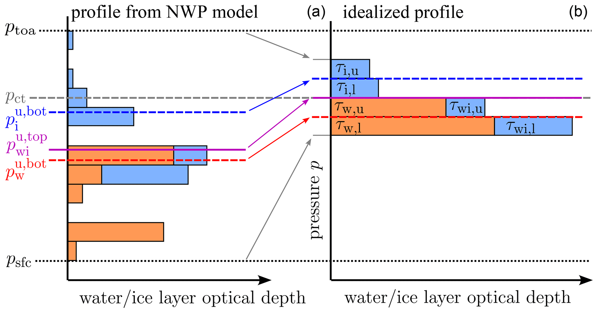
Figure 5 Schematic example of a complex profile from an NWP model (a) and the corresponding idealized profile (b) in which only four layers are filled with clouds. The dashed blue and red lines separate the upper and lower parts of the ice and the mixed-phase cloud, respectively. The purple line separates pure ice from mixed-phase ice. The dashed grey line indicates the cloud top pressure and the dotted black line the surface pressure. The pressure labels correspond to the geometric heights z with the same indices defined in the text. The thickness of the layers is exaggerated; the four cloud layers in the idealized profile are all close to p_ct.

Using the idealized profiles instead of the NWP model profiles as input for DOM will lead to reflectance errors, which should decrease with the number of parameters used to characterize the idealized profiles. In the following, we discuss the relative importance of the new input parameters by using different profile data sets (see Table 1) and different profile simplifications. Which profiles were used as input for DOM to compute reflectances are indicated by the following indices:

•  

  DOM – full non-idealized profiles (reference solution);

•  

  2Lay,mp – idealized profiles characterized by the 16 input parameters in p;

•  

  2Lay – like 2Lay,mp but all ice is moved to the pure ice cloud (12 parameters);

•  

  1Lay – like 2Lay but using only one layer per cloud (10 parameters);

•  

  1Lay,fix – like 1Lay but the cloud top and base are set to fixed heights, no IWV (7 parameters).

For 2Lay, 1Lay and 1Lay,fix the integration ranges are chosen such that all ice ends up in the pure ice cloud ($z_{\mathrm{i}}^{\text{l,bot}}=z_{\text{wi}}^{\text{u,top}}=z_{\text{sfc}}$). The 1Lay,fix setup corresponds to the original MFASIS from Scheck et al. (2016), and the same fixed cloud top and base heights are also adopted.

3.2 Impact of surface pressure and cloud top height

To quantify the impact of taking p_ct, p_sfc and IWV into account, it is helpful to exclude other sources of reflectance error. For this purpose, the data sets w-rconst and i-rconst (see Table 1) are used, which contain only clouds of one phase with vertically constant effective radii. Errors related to mixed-phase clouds and vertical radius gradients are thus excluded, but errors related to the simplification of the vertical cloud/clear-sky structure are present. These errors should be smaller when in the idealized profiles p_ct and p_sfc have the same value as in the original profile so that approximately the same air masses above and below the cloud top influence the reflectance by molecular absorption and Rayleigh scattering. In the absence of vertical radius gradients it is sufficient to consider one-layer clouds, and we therefore compare reflectances computed with the cloud top and surface pressures from the original profile, R_1Lay, to the ones computed with fixed cloud top and surface pressures, R_1Lay,fix, which uses the same idealized profiles as in Scheck et al. (2016). The mean absolute errors $|R_{\text{1Lay}}-R_{\text{DOM}}|$ and $|R_{\mathrm{1}\mathrm{Lay},\mathrm{fix}}-R_{\text{DOM}}|$ with respect to the reference solution for both water and ice clouds are shown in Fig. 6 as a function of optical depth and the maximum of the zenith angles.

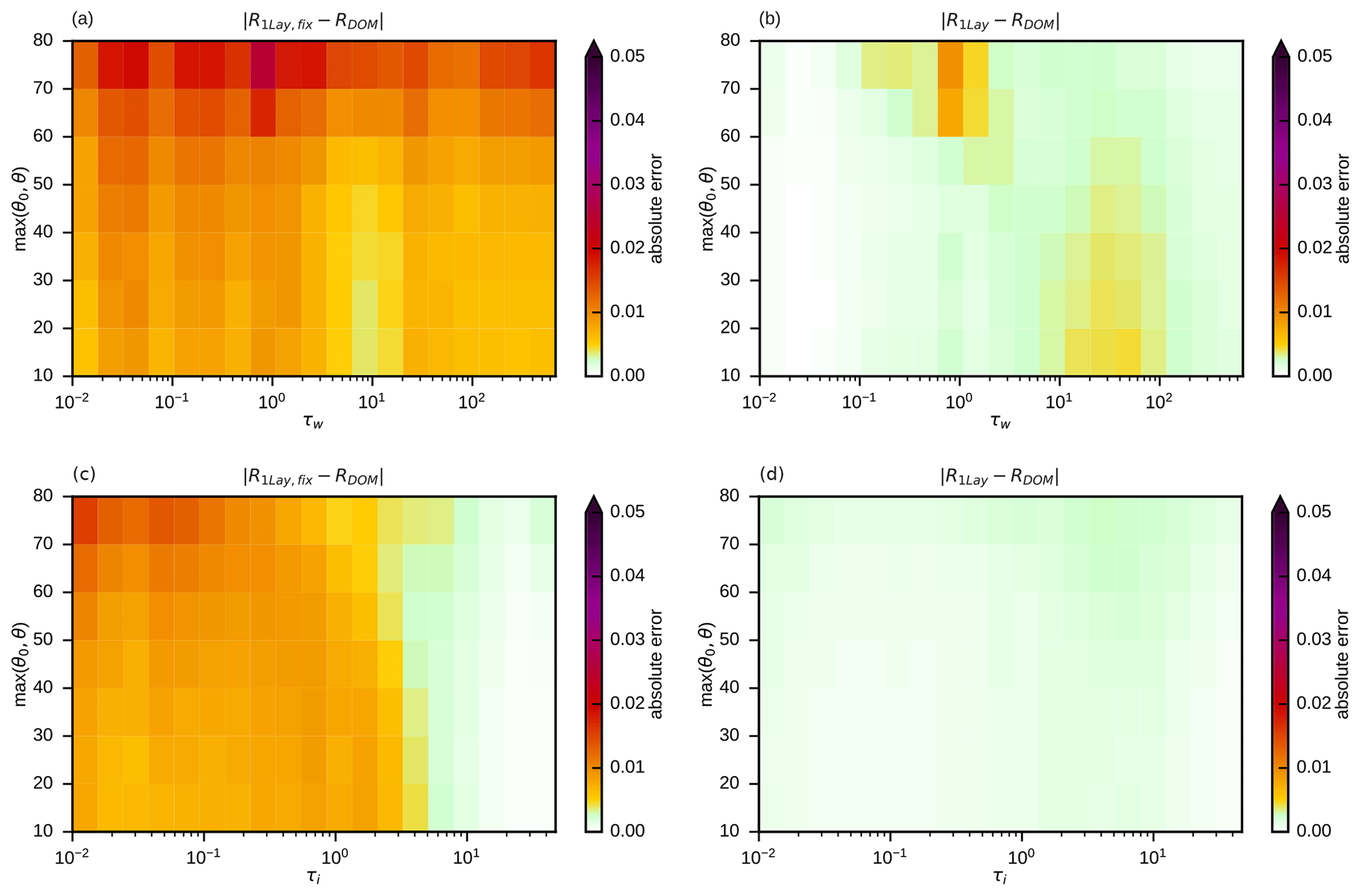
Figure 6 Mean absolute reflectance errors for simplified profiles without (a, c) and with (b, d) taking cloud top and surface pressure into account with respect to the DOM reference solution for the full profiles of the w-rconst (a, b) and i-rconst (c, d) data sets in bins defined by optical depth and the maximum of solar and satellite zenith angles.

The errors for the water clouds (Fig. 6a and b) are higher than for the ice clouds (Fig. 6c and d), as for clouds located at lower heights the air masses and their impact on reflectance are higher. Larger zenith angles also lead to a stronger influence of molecular absorption and Rayleigh scattering and thus higher errors in Fig. 6, as they increase the photon path lengths. For both data sets a clear error reduction (Fig. 6a and b; Fig. 6c and d) is visible when p_ct, p_sfc and IWV are taken into account. In particular, errors at higher optical depths are reduced (τ_w>100, τ_i>10), but at intermediate optical depths (τ_w=10…100, τ_i=1…10) significant error reduction can also be observed. For ice clouds, the remaining mean absolute errors are of the order 𝒪(10⁻³), i.e. very small (Fig. 6d). For water clouds, the errors at τ_w>100 are reduced to similarly low levels (Fig. 6b). For water clouds of intermediate optical depths, errors are reduced considerably, but mean absolute errors around 0.01 can still be found when p_ct and p_sfc are taken into account. However, these errors are already in an acceptable range. In fact, for both data sets, only 15 % of the original mean absolute error (MAE) and 25 % of the extreme errors (P99) remain (see Table 3).

3.3 Optimizing two-layer clouds

In Sect. 3.1 two-layer clouds are introduced as a simple way to approximate the effect of vertical effective radius gradients. How the clouds in the idealized profiles should be split up in an upper and a lower layer still has to be defined. For optically thin clouds the probability of a photon to be scattered in the upper or the lower half (in terms of optical depth) of the cloud should be similar, so it makes sense to split them such that ${\mathit{\tau }}_C^{\mathrm{u}}={\mathit{\tau }}_C^{\mathrm{l}}$ (where C=w for water and C=i for ice clouds) and to compute mean effective radii for the upper and lower half. For denser clouds the contribution of layers deeper in the cloud to the top-of-atmosphere reflectance should be smaller due to absorption. To resolve the effective radius gradient in regions where it has the strongest impact on the reflectance, it would in this case be more appropriate to split the clouds in a thinner upper part and a thicker lower part. The optimal optical depth to split at depends of course also on the vertical effective radius profile. We assume that a parameterization for a splitting factor $f_C=\frac{{\mathit{\tau }}_C^{\mathrm{u}}}{{\mathit{\tau }}_C}$ can be found that works reasonably well for many different effective radius profiles, where ${\mathit{\tau }}_C={\mathit{\tau }}_C^{\mathrm{u}}+{\mathit{\tau }}_C^{\mathrm{l}}$ is the total optical depth of the two-layer cloud. From the argumentation above, the parameterization should produce a value of $\frac{\mathrm{1}}{\mathrm{2}}$ for small optical depths and decline with increasing τ_C. However, the zenith angles should also play a role because they influence the path length in the cloud and thus also the probability of a photon to be absorbed. For the sake of simplicity, we use the single parameter ${\mathit{\theta }}_m=max({\mathit{\theta }}_{\mathrm{0}},\mathit{\theta })$, the maximum of the two zenith angles, to quantify the zenith angle dependence. For determining a reasonable function f_C(τ_C,θ_m), the mean error reduction $|R_{\text{1Lay}}-R_{\text{DOM}}|-|R_{\mathrm{2}\mathrm{Lay}}-R_{\text{DOM}}|$ was computed for the w-only and i-only data sets and many different bins defined by f_C, τ_C and θ_m. As an example, the case $\mathrm{60}{}^{\circ }<{\mathit{\theta }}_m<\mathrm{70}$^∘ for ice clouds is shown in Fig. 7. It is obvious that for low optical depths, where exactly the cloud is split does not make much of a difference and that with increasing optical depth the error can be reduced more strongly when smaller values of f_C are chosen.

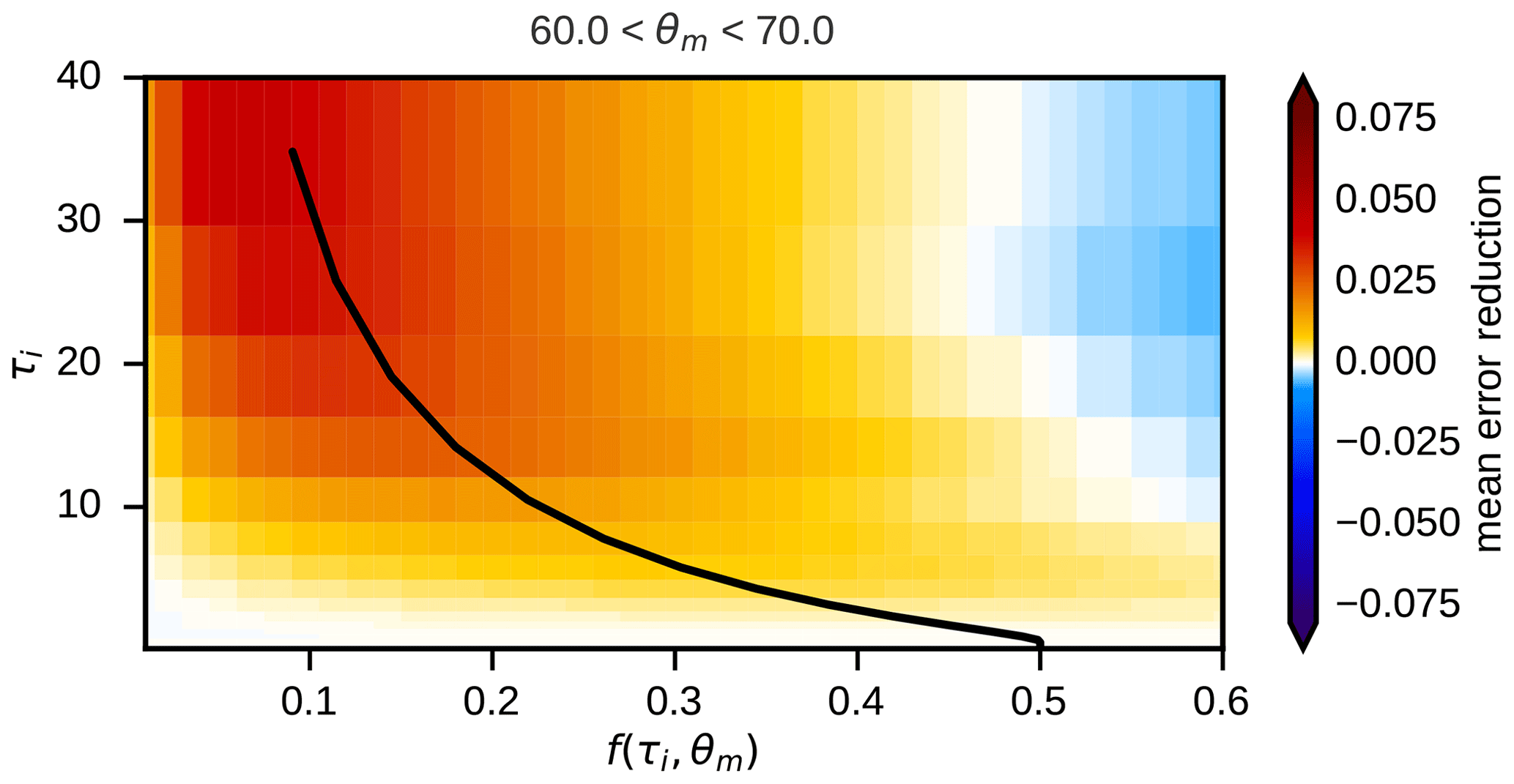
Figure 7 Mean absolute reflectance error reduction $|R_{\text{1Lay}}-R_{\text{DOM}}|-|R_{\mathrm{2}\mathrm{Lay}}-R_{\text{DOM}}|$ achieved by using two-layer clouds instead of one-layer clouds for the i-only data set for different values of the layer splitting factor f_i and the optical depth τ_i in the zenith angle bin $\mathrm{60}{}^{\circ }<{\mathit{\theta }}_m<\mathrm{70}{}^{\circ }$. Positive values mean the two-layer approach is better than the one-layer approach. The splitting factor parameterization as defined in Eq. (8) is visualized by the white line.

A function producing near-optimal values for the splitting factor is given by

$$\begin{array}{}\text{(8)}& \begin{array}{rl}{f}_C& ({\mathit{\tau }}_C,{\mathit{\theta }}_m)=\\ & {\displaystyle \frac{\mathrm{1}}{\mathrm{2}}}-\left[{\displaystyle \frac{\mathrm{1}}{\mathrm{2}}}-f_{\mathrm{hi}}\left({\mathit{\theta }}_m\right)\right]\times {\displaystyle \frac{\mathrm{1}}{\mathrm{2}}}\left[\mathrm{1}-\cos \left(\mathit{\pi }{t}_C\right({\mathit{\tau }}_C\left)\right)\right],\end{array}\end{array}$$

where

$$\begin{array}{}\text{(9)}& t_C\left({\mathit{\tau }}_C\right)=min\left(\mathrm{1},max\left(\mathrm{0},{\displaystyle \frac{\log \left({\mathit{\tau }}_C\right)-\log \left({\mathit{\tau }}_{C,\text{lo}}\right)}{\log \left({\mathit{\tau }}_{C,\text{hi}}\right)-\log \left({\mathit{\tau }}_{C,\text{lo}}\right)}}\right)\right),\end{array}$$

with ${\mathit{\tau }}_{\mathrm{i},\mathrm{lo}}=\mathrm{0.6}$, ${\mathit{\tau }}_{\mathrm{i},\mathrm{hi}}=\mathrm{75}$ for ice clouds and ${\mathit{\tau }}_{\mathrm{w},\mathrm{lo}}=\mathrm{1.0}$, ${\mathit{\tau }}_{\mathrm{w},\mathrm{hi}}=\mathrm{500}$ for water clouds and the zenith-angle-dependent term

$$\begin{array}{}\text{(10)}& f_{\mathrm{hi}}\left({\mathit{\theta }}_m\right)=f_{\mathrm{zen}}-{\displaystyle \frac{{\mathit{\theta }}_m}{{\mathrm{90}}^{\circ }}}\mathrm{\Delta }{f}_{\mathrm{hor}},\end{array}$$

with f_zen=0.1 and Δf_hor=0.05. The constants used in the definition of f_C(τ_C,θ_m) are chosen such that in plots like Fig. 7 for all angle bins and both water and ice clouds the parameterization yields a value of the splitting factor that is close to maximizing the error reduction, as illustrated by the example in Fig. 7 (black line). For both water and ice clouds the parameterized splitting factors start at $\frac{\mathrm{1}}{\mathrm{2}}$ for low optical depths, decrease with increasing depth and saturate at the same value for high optical depths (Fig. 8). For ice clouds, which are optically considerably thinner than the water clouds (see Fig. 1), the decline takes place at lower optical depths.

For testing the two-layer approach, the data sets w-only and i-only are considered, which do not contain mixed-phase clouds but have vertically varying effective radii. For both data sets the mean absolute errors for the one-layer approach with surface and cloud top pressure taken into account are considerably worse than for the corresponding data sets without vertical radius gradients (compare Fig. 6b to Fig. 9a and Fig. 6d to Fig. 9c, and see Table 3). In particular for optical depths larger than 10 reflectance errors exceeding 0.05 can be found. Switching from the one-layer to the two-layer approach with the parameterized splitting factors reduces the error considerably (compare Fig. 9a and b as well as c and d) at these moderate to high optical depths. The remaining errors are around 0.01 or lower in most parts of the parameter space; only for large zenith angles and very high optical depths can somewhat larger values be found (Fig. 9b and d).

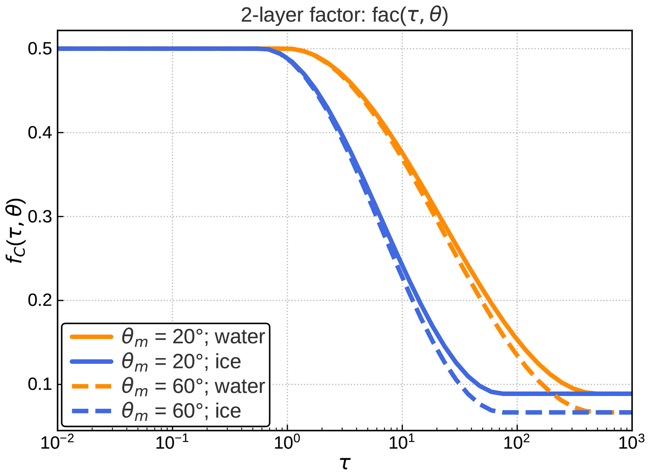
Figure 8 The two-layer splitting factor parameterization f_C(τ_C,θ_m) for water (orange) and ice clouds (blue) as a function of the optical depth and for two different values of the zenith angle parameter, θ_m=20^∘ (solid) and θ_m=60^∘ (dashed).

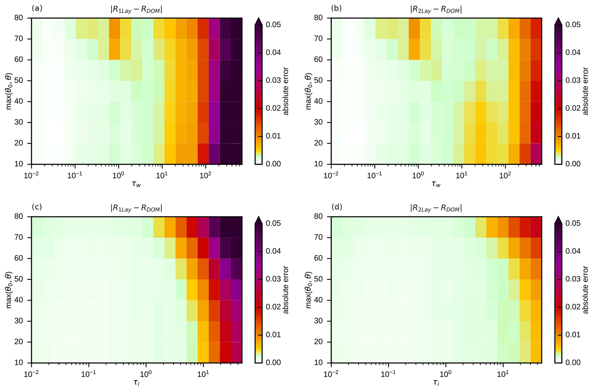
Figure 9 Mean absolute reflectance errors for simplified profiles with one-layer (a, c) and two-layer clouds (b, d) with respect to the DOM reference solution for the full profiles of the w-only (a, b) and i-only (c, d) data sets in bins defined by optical depth and the maximum of solar and satellite zenith angles. In all cases cloud top and surface pressure were taken into account.

3.4 Accounting for mixed-phase clouds

So far, only data sets without mixed-phase clouds have been used. For the std data set including mixed-phase clouds, the two-layer approach without special treatment of mixed-phase clouds results in strongly increased errors. The mean absolute reflectance error, now computed for bins of the total optical depth of all water and ice layers in the column, τ_t, and the zenith angle parameter θ_m can exceed 0.05 for high optical depths (Fig. 10a), which is considerably higher than errors for pure water (Fig. 9b) and pure ice clouds (Fig. 9d). The misrepresentation of mixed-phase clouds can thus cause errors that are similar in size to the ones related to not taking vertical effective radius gradients into account. By allowing for mixed-phase ice in the two layers of the mixed-phase cloud in the idealized profiles, as discussed in Sect. 3.1, these errors can be reduced significantly. As shown in Fig. 10b, the mean absolute reflectance errors are around 0.01 or lower in most of the parameter space.

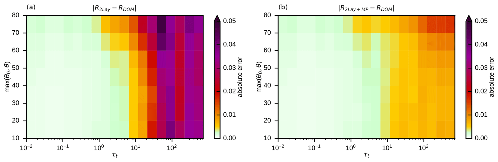
Figure 10 Mean absolute reflectance errors for simplified profiles without (a) and with (b) special treatment of mixed-phase clouds with respect to the DOM reference solution for the full profiles of the std data set in bins defined by total optical depth and the maximum of solar and satellite zenith angles. In all cases cloud top and surface pressure were taken into account, and two-layer clouds were used.

3.5 A simple bias correction

Most of the remaining mean absolute error in Fig. 10b is actually not a random error but related to a mean error or bias, as is evident from Fig. 11a. A part of the bias may depend on details of the profile data set and the effective radius parameterizations used here. However, most of it may be independent of the details and directly related to the profile simplifications and therefore would still be present for a “perfectly realistic” data set. To confirm this conjecture it seems worthwhile to develop a simple bias correction to remove most of the remaining mean errors for the std data set and investigate later on if the correction is helpful for other data sets. Due to the clear structure of the bias it is easy to derive a simple function of the total optical depth and the zenith angle parameter θ_m, which reproduces the mean error. Here we use a Gaussian-shaped correction

$$\begin{array}{}\text{(11)}& \mathrm{\Delta }{R}_{\mathrm{bc}}({\mathit{\tau }}_{\mathrm{t}},{\mathit{\theta }}_m)={\displaystyle \frac{m+n\times ({\mathit{\theta }}_m/\mathrm{90}{}^{\circ }{)}^k}{\sqrt{\mathrm{2}\mathit{\pi }}{\mathit{\tau }}_{\mathrm{t}}\mathit{\sigma }\exp \left(-\frac{\left(\log \right({\mathit{\tau }}_{\mathrm{t}})-\mathit{\mu }{)}^{\mathrm{2}}}{\mathrm{2}{\mathit{\sigma }}^{\mathrm{2}}}\right)}}\end{array}$$

with the parameters ($\mathit{\sigma }=\mathrm{1.1},\mathit{\mu }=\mathrm{7},m=\mathrm{12},n=\mathrm{30},k=\mathrm{3.5}$) chosen such that the correction predominantly acts for τ_t larger than approximately 50. As Fig. 11b shows, applying the bias correction to the std data set removes most of the bias and reduces the MAE by 25 % and the P99 by about 20 % (see Table 3). For the rmod data set using different effective radius parameterizations, the bias correction (Fig. 11c) also still reduces the MAE and the P99 by about 20 % (see Table 3). The fact that the bias correction reduces errors for both data sets indicates that it does not depend strongly on details of the std data set and that it seems to correct a more generic error related to the profile simplification.

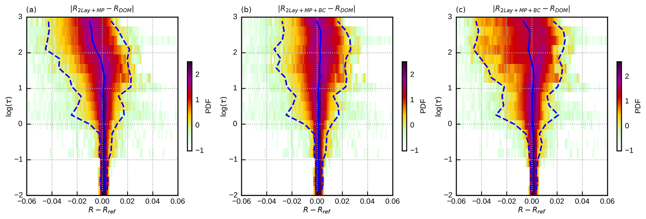
Figure 11 Error probability density functions (PDFs; shaded) showing the deviation of different reflectance estimations (R) from DOM reference computations (R_ref) as a function of optical depth (log(τ)). These are not 2D PDFs – each horizontal cut through these images represents the 1D PDF for the optical depth bin indicated on the vertical axis. The dashed blue lines depict the 1st (left) and 99th (right) percentiles of the error, while the solid blue line shows the mean error. The error histograms are shown for 2Lay+MP (a) of the standard data set, as well as for 2Lay+MP+BC of the standard (b) and rmod (c) data sets.

4 Network training

As discussed in the previous section, replacing vertical profiles from NWP model runs by the corresponding idealized profiles characterized by the same parameters results in only small reflectance errors. These profile parameters are thus in principle suitable as input parameters for a neural network to predict reflectances.

4.1 Setup

The function to be learned by the neural network is similar but due to the additional parameters somewhat more complex than in the case of the visible channel investigated in Scheck (2021a). Therefore, we will investigate for the near-infrared channel if networks of a similar or slightly larger size as considered for the visible channel can be trained with similar training settings to achieve comparable reflectance errors. In this section only errors due to imperfect training of the networks will be considered but not the errors caused by simplifying the vertical structure, which have been discussed in the previous section. Therefore, the R_2Lay,mp reflectances computed with DOM for idealized profiles with randomly chosen parameters will serve as training and validation data. About 30 million samples, i.e. tuples of input parameters and reflectances, were generated for this purpose.

In Fig. 12 an example for the network structure is shown. The nodes of the input layer correspond to the elements of p (defined in Eq. 7) describing the idealized profiles and the sun–satellite geometry. The range applied for the parameters is listed in Table 2. There is no input node for the surface albedo, as the latter is treated in a different way. As discussed in more detail in Scheck (2021a), in plane-parallel RT the reflectance for an arbitrary albedo value can be computed exactly if reflectances for three different values are known. If the network is trained to generate reflectances for three different albedo values, albedo is thus not required as an input parameter, and errors resulting from an imperfect representation of the albedo dependence by the network can be avoided. Following Scheck (2021a), the reflectance for albedo zero, R(0), and the reflectance differences, $D_{\frac{\mathrm{1}}{\mathrm{2}}}=R\left(\frac{\mathrm{1}}{\mathrm{2}}\right)-R\left(\mathrm{0}\right)$ and $D_{\mathrm{1}}=R\left(\mathrm{1}\right)-R\left(\frac{\mathrm{1}}{\mathrm{2}}\right)$, are chosen as output parameters, where R(A) is reflectance as a function of surface albedo A. These differences are used instead of $R\left(\frac{\mathrm{1}}{\mathrm{2}}\right)$ and R(1) because the computation of reflectance for an arbitrary A requires $R\left(\mathrm{1}\right)>R\left(\frac{\mathrm{1}}{\mathrm{2}}\right)>R\left(\mathrm{0}\right)$ to avoid numerical problems, and by using softplus as an activation function for the output nodes the constraints R(0)>0, D_½>0 and D₁>0 are automatically fulfilled. Following the TensorFlow standard approach, the root-mean-square error (RMSE) of all of the network output variables, ϵ_TF, is minimized in the training.

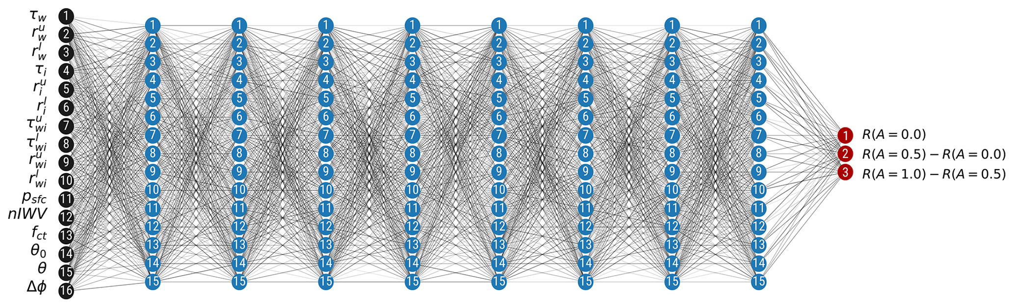
Figure 12 Structure of the smallest network considered, with 16 input nodes (black), 8 hidden layers with 15 nodes per layer, and in total 1983 weight and bias parameters. As activation functions (see Sect. 2.1.3), CSU (Eq. 1) is used for the hidden layers (blue nodes) and softplus for the output layer (red nodes). The lines in different shades of grey symbolize the network weights.

Table 2 List of input parameters for the neural networks, their abbreviation and their range.

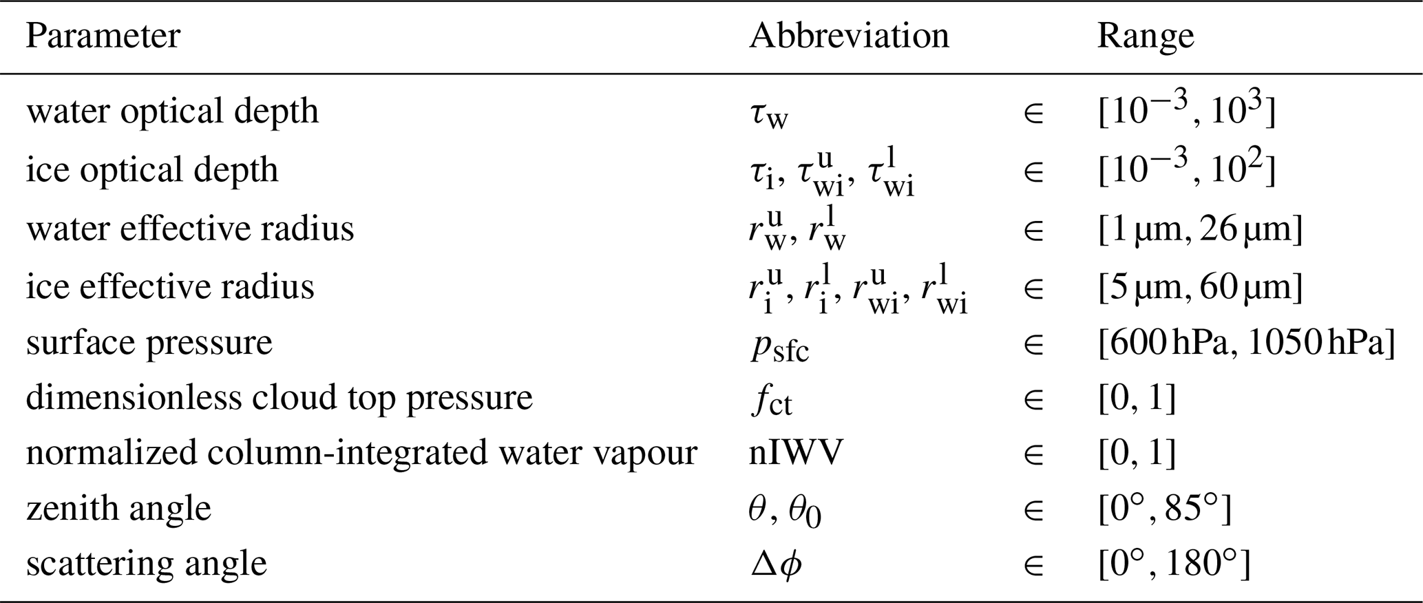
In contrast to Scheck (2021a), we will not explore the full parameter space of training- and network-related settings, but we show only that for a plausible choice of training and network structure settings sufficiently accurate networks result. Only the most relevant setting for the network structure is varied, which is the total number of parameters. For the visible channel, networks with 2000 parameters already resulted in acceptable reflectance errors that were somewhat smaller than the interpolation errors in the LUT version, and for 5000 parameters the errors were negligible compared to the error caused by the profile simplification (Scheck, 2021a). Here we investigate networks with 1983 (NN2k), 5053 (NN5k) and 8035 (NN8k) parameters, which are trained for 4000 epochs using 14×10⁶ training samples.

4.2 Results

From Fig. 13, which shows the evolution of the RMSE of the output parameters, ϵ_TF, during the training of the three networks, it is obvious that for all of them errors of several 10⁻³ are reached for both the training and the validation data sets. Due to the early-stopping strategy the errors for the validation data set are somewhat smaller than for the training data set. The final errors provided in Fig. 13 suggest that a number of parameters between 2000 and 5000 may be a reasonable choice, and not much accuracy is gained by further increasing the number of parameters. It should be noted that the NN8k network shows the first signs of overfitting – a small gap appears between the training data and the validation data after about 2000 epochs. Further training of NN8k would thus require larger amounts of training data. For the smaller networks the amount of training data seems to be sufficient. The choice of the network size should of course also depend on the computational costs for evaluating networks of different sizes. Benchmarks for different network sizes and activation functions have already been investigated for the optimized FORNADO inference code (see Fig. A12 in Scheck, 2021a). Evaluating the 1983, 5053 and 8035 parameter networks considered here takes 0.14, 0.30 and 0.51 µs per column, respectively, on a core of a standard Intel Xeon 8358 server CPU running at 3.3 GHz. For comparison, the lookup-table-based MFASIS (using the LUT with $N_k=N_l=\mathrm{3}$; see Table 3 of Scheck et al., 2016) takes 1.58 µs, and the DOM implementation in RTTOV (with 16 streams) takes about 17 ms per column on the same CPU. These timings are only for the computation of reflectances from the input parameters⁵ listed in Table 2. Although some additional effort is required for computing the network input parameters from the NWP profiles, it should be possible to process e.g. 10⁶ model columns in several CPU seconds with these networks.

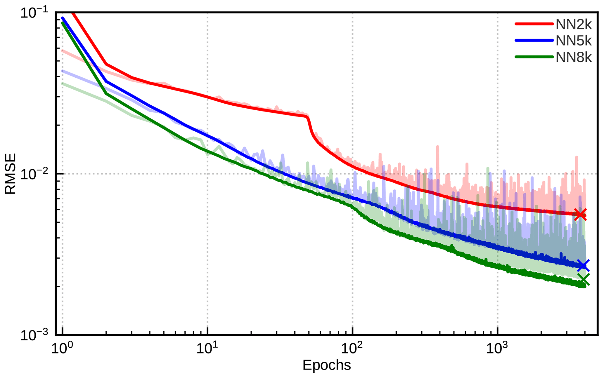
Figure 13 Evolution of the training (solid colour) and validation (light colour) RMSEs during the course of the training for a networks with 1983 (NN2k, red), 5053 (NN5k, blue) and 8053 (NN8k, green) parameters. The final validation RMSE values for each network (indicated by the crosses) are $\mathrm{5.6}\times {\mathrm{10}}^{-\mathrm{3}}$ (NN2k), $\mathrm{2.7}\times {\mathrm{10}}^{-\mathrm{3}}$ (NN5k) and $\mathrm{2.2}\times {\mathrm{10}}^{-\mathrm{3}}$ (NN8k).

The networks and training procedures discussed here are not yet fully optimized. Further gains in accuracy could be expected e.g. from tuning the learning rate, the batch size and the number of hidden layers. In addition, regularization techniques could make the training more efficient, and using a lower-precision data type, e.g. 16 bit instead of 32 bit floating point values, could speed up training and inference. However, such tuning efforts are not in the scope of this study, and in their current state the neural networks already seem to be sufficiently fast and accurate.

5 Evaluation

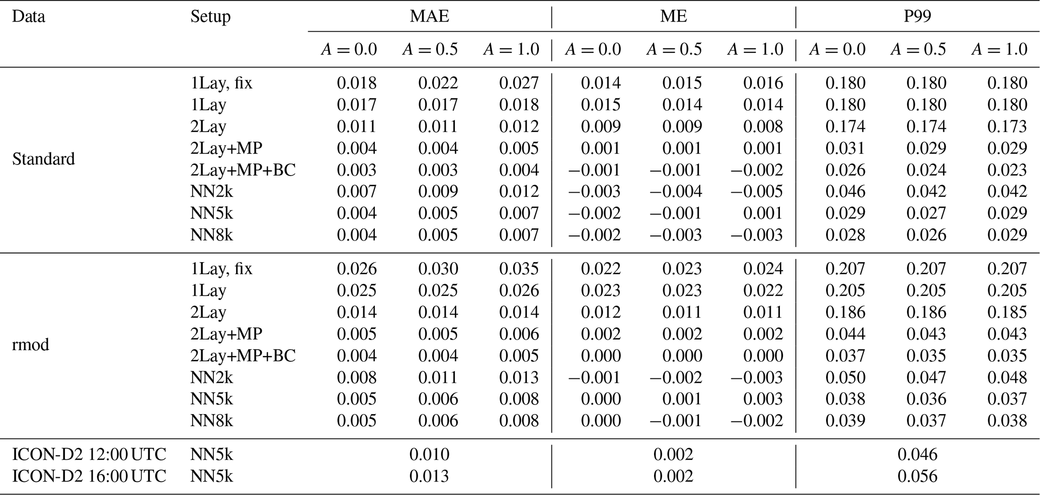
In the previous sections, the reflectance errors related to simplifying vertical profiles and using neural networks instead of applying the DOM reference RT method to the simplified profiles have been discussed separately. We now investigate the total error and the relative importance of simplification and neural network errors also using vertical profiles that are different from those that have been used so far. To provide an overview of all considered cases, values for the mean absolute error (MAE), the mean error (ME) and the 99th percentile of the absolute error (P99) are listed in Table 3.

Table 3 Error statistics for all data sets (the ones from Table 1 and the ICON hindcasts for 12:00 and 16:00 UTC), DOM computations for idealized profiles with different numbers of parameters (see Sect. 3.1) and three differently sized neural networks. +BC means that the bias correction from Sect. 3.5 was applied. Listed are the mean absolute error (MAE), the mean error (ME) or bias, and the 99th percentile of the absolute error (P99). For each metric three values are provided, which correspond to the albedo values A=0.0, 0.5 and 1.0. The ICON-D2 hindcasts are an exception – here we used for each profile only the actual albedo value.

5.1 NWP SAF profiles

The mean absolute reflectance error for the std profile data set with surface albedo A=0.5 is shown in Fig. 10b as a function of the total optical depth and the maximum of the zenith angles, and the error is shown in Fig. 11b as a function of total optical depth. Here we investigate the full error distribution and discuss the relative impacts of the different input parameters and compare them to the effect the neural network errors have on the distribution. The reflectance error distributions of DOM computations with simplified profiles, R_1lay,fix, R_1lay, R_2lay, R_2lay,mp and $R_{\mathrm{2}\mathrm{lay},\mathrm{mp},\mathrm{bc}}$, and neural network calculation R_NN5k are shown in Fig. 14 for the std and rmod data sets and different albedo values. In addition, values for the mean absolute error (MAE), the mean error (ME) and the 99th percentile of the absolute error (P99) are provided in Table 3.

It is quite obvious from the distribution plots and the metrics in Table 3 that DOM computations based on the 1Lay,fix idealized profiles (the original approach from Scheck et al., 2016) result in rather large errors, in particular on the left side of the histograms in Fig. 14 (light blue curves). Including surface pressure, cloud top pressure and integrated water vapour improves the distribution significantly for positive reflectance errors but not for the large negative errors (orange curves). Consequently, these improvements, which are related to profiles with high amounts of water vapour, result only in a reduction in the MAE but not P99. The strongest MAE reductions are seen for A=1, which can be expected, as in this case a wrong amount of water vapour leads to the largest error in the radiance reflected from the surface. Applying the two-layer approach (2Lay, purple curves) leads to further improvements for negative reflectance errors, resulting in lower mean and mean absolute errors for all albedo values and both data sets. However, as many cases with large reflectance underestimation are still present, P99 still remains high. Improving the representation of mixed-phase clouds (2Lay+MP, red curves) basically removes all the extreme cases with negative errors and reduces the P99s by about 80 % and the mean errors to very low levels. In 2Lay+MP, dark mixed-phase ice is often located below brighter water clouds, which leads to higher reflectances than in 2Lay, where all ice is always located above the water cloud. As already shown in Fig. 11, the remaining negative errors partly result from a optical-depth-dependent bias. By applying the simple bias correction from Sect. 3.5, the cases with larger errors are shifted to the right in the histograms (Fig. 14, green curves) without changing the position of the peak. Consequently, all metrics are slightly improved.

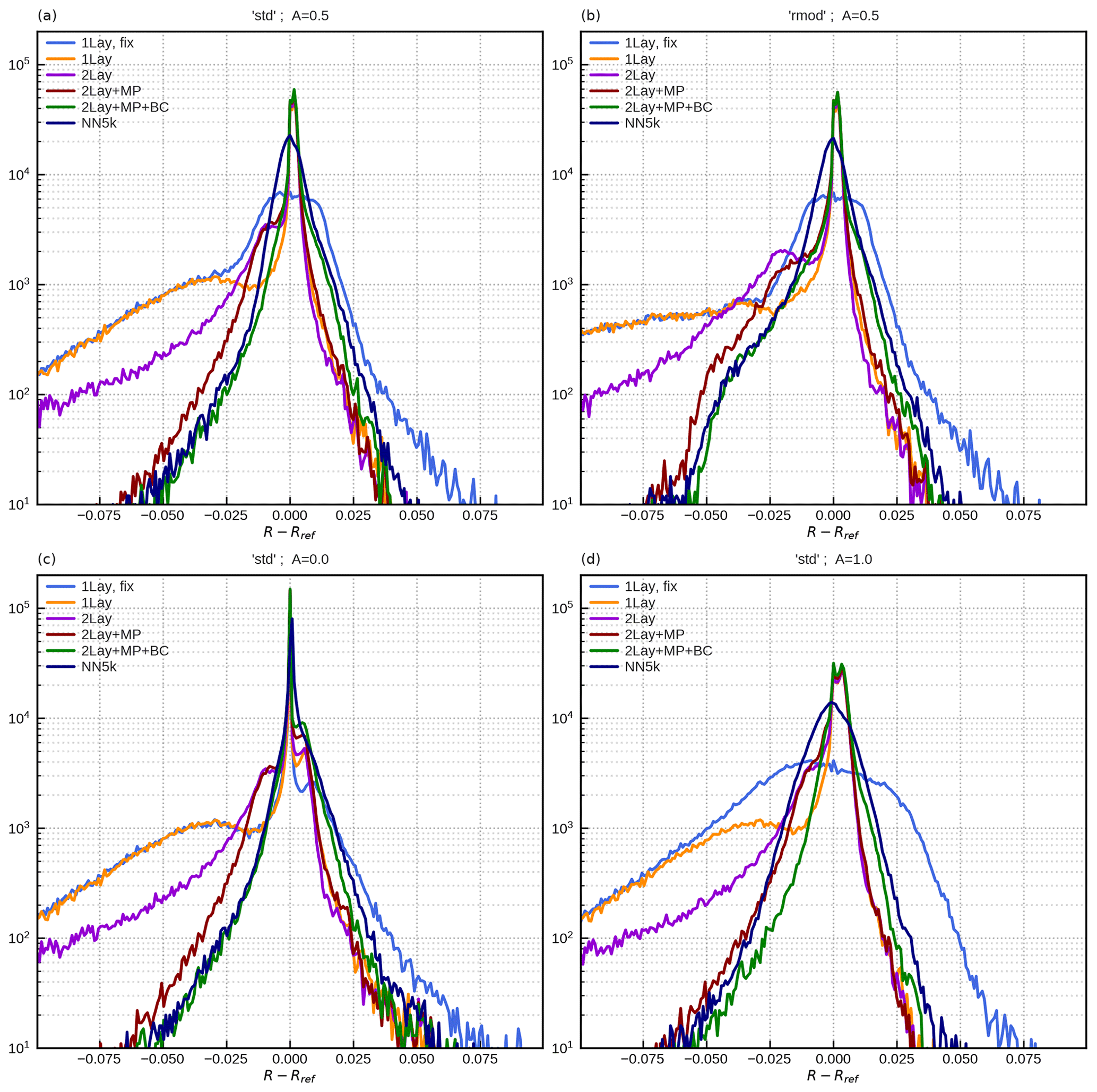
Figure 14 Error histogram showing the deviation of different reflectance estimations (R) from DOM reference computations (R_ref). Shown are estimations calculated using 1Lay,fix (light blue), 1Lay (orange), 2Lay (purple), two-layer parameterization adding mixed-phase clouds (2Lay+MP, red), and two-layer parameterization adding mixed-phase clouds and bias correction (2Lay+MP+BC, green), as well as the realization using the trained neural network (NN5k, dark blue). The different panels show the standard data (std) set applying albedo 0.5 (a), 0.0 (c) and 1.0 (d). Furthermore, rmod is shown for an albedo of 0.5 in panel (b).

Comparing the computations with simplified profiles to results for the neural network NN5k (dark blue curves) shows that the additional network errors are small compared to the simplification errors. In fact, the changes in histograms due to additional NN errors are in most cases smaller than the ones caused by the bias correction. Only for A=1 a somewhat stronger impact of the NN errors is visible. Results for the NN2k and NN8k networks (only included in Table 3, not in Fig. 14) show that the smaller 1983 parameter network causes non-negligible additional errors, whereas the larger 8053 parameter network does not lead to significantly improved error metrics.

5.2 Regional ICON hindcasts

The results of the previous section show that our approach also works if effective radius parameterizations that are different from the ones employed for defining the two-layer splitting factor parameterizations and the bias correction are used. In the following, we investigate profiles from a different NWP model, the regional ICON-D2 model, and use effective radii determined by the two-moment microphysics scheme in the model.

We focus on synthetic SEVIRI 1.6 µm images of the ICON-D2 domain at 12:00 and 16:00 UTC in a 30 d test period (June 2020). For each date and time, images were computed using both DOM and the NN5k network. In total, almost 14×10⁶ test cases per time step are available for each time to compare DOM and the NN. As an example, Fig. 15a depicts the synthetic satellite image computed using NN5k for 4 June 2020 at 12:00 UTC. Compared to the DOM reference method, the errors in NN5k are predominantly below 0.04 (Fig. 15b), which is in a similar range as for the std and rmod data sets.

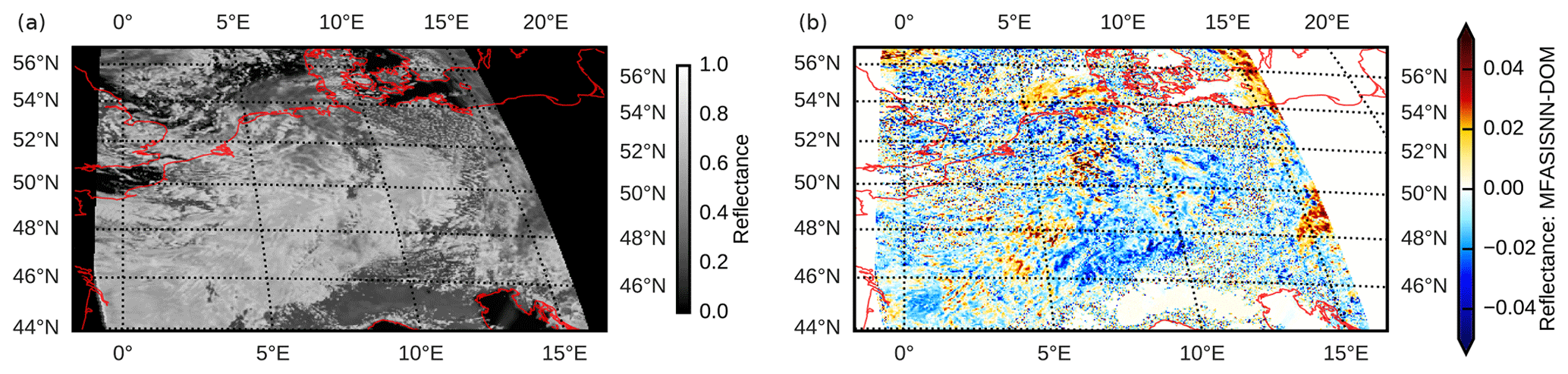
Figure 15 (a) Synthetic satellite image computed using the neural network NN5k for the ICON-D2 domain on 4 June 2020 at 12:00 UTC and (b) its deviation from the reference DOM computation.

These results confirm the robustness of our approach. Although a completely different model and supposedly more realistic (and certainly different) effective radii are used, the errors are only increased slightly compared to the ones computed for the IFS profile collection, which was also used for the development and optimization of the approach.

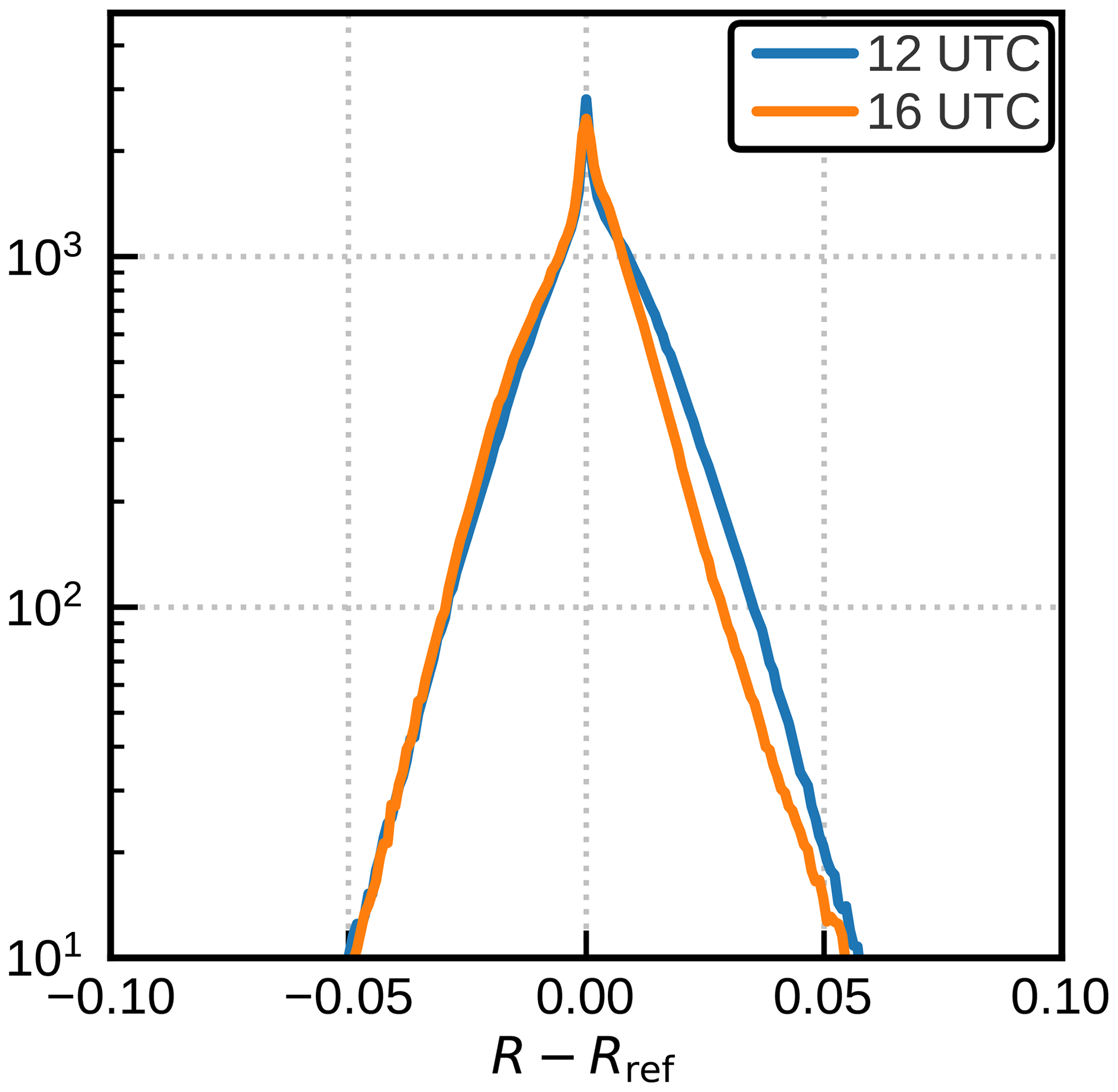
The error distribution for all 12:00 and 16:00 UTC images of the test period (Fig. 16) is similar to the one for the rmod IFS profile data set (compare to Fig. 14b, blue line). The mean absolute error (MAE) and P99 errors for the ICON-D2 case are only slightly higher, but the overall mean error (ME) is similarly small (also see Table 3). The P99 for 16:00 UTC, when the solar zenith angle is larger, is only slightly worse.

Figure 16 Error histogram showing the deviation of NN5k from the DOM reference computations. Data are sampled over the complete domain (see Fig. 15) for 12:00 UTC (blue) and 16:00 UTC (orange). This data set amounts up to about 4.5×10⁶ cloudy pixels.

5.3 Other solar channels

The method developed here for the 1.6 µm SEVIRI will not provide satisfactory results for all solar channels. However, for many visible and near-infrared channels the errors are in a similar range as for the 1.6 µm channel. To illustrate for which channels our method is usable, we consider all purely solar channels (we will not consider channels with thermal contributions like 3.7–3.9 µm channels) of the current and next-generation EUMETSAT satellite imagers. These are SEVIRI on MSG, the Flexible Combined Imager (FCI) on Meteosat Third Generation (MTG), the Advanced Very High Resolution Radiometer (AVHRR) on the EUMETSAT Polar System (MetOp) and Meteorological Imager (METimage) on MetOp Second Generation. The root-mean-square profile simplification error computed with the IFS profile collection for these channels is shown in Fig. 17. From these results it is obvious that all channels with wavelengths up to 0.7 µm and many channels with larger wavelengths up to 2.2 µm have errors similar to or smaller than the 1.6 µm channel. In particular, the stronger absorption by clouds in the case of the 2.2 µm channel does not seem to be a problem. While stronger Rayleigh scattering could in principle pose an additional challenge for channels with small wavelengths, the error for these channels is actually smaller than for the 1.6 µm channels. It seems that the cloud top pressure and surface pressure input variables originally introduced to quantify the absorption by CO₂ and CH₄ also characterize the Rayleigh scattering sufficiently well. For those cases with a profile simplification RMSE smaller than 0.01, we also trained neural networks, and the full reflectance RMSE (due to profile simplification and imperfect network training) is shown as crosses in Fig. 17. We did not train all networks for the same number of epochs, and in some cases we used networks with only 2000 and not 5000 parameters, which results in some variation in the additional error related to the network training. In none of the cases does the full reflectance RMSE exceed 0.012, and further optimizations seem possible.

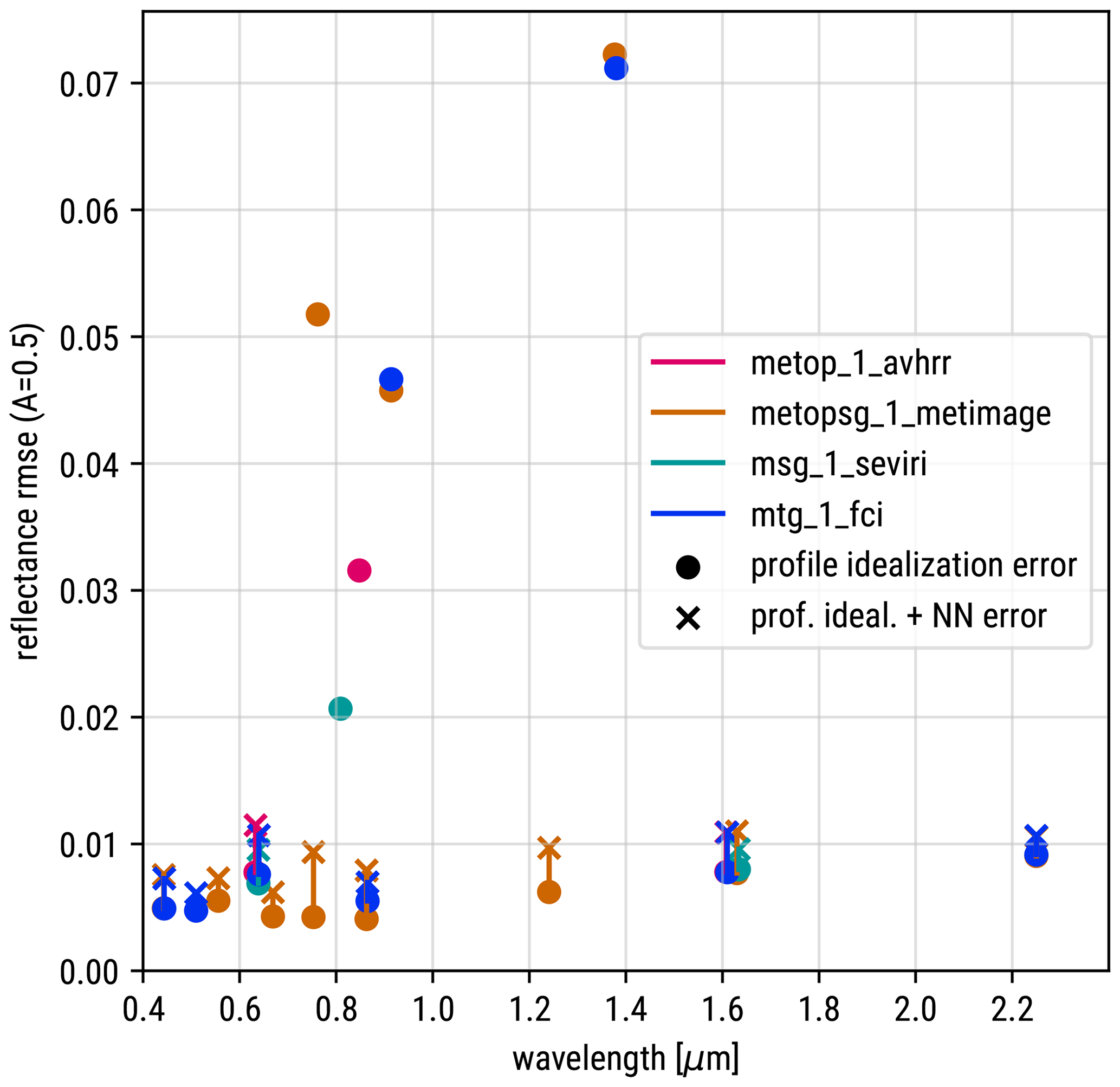
Figure 17 Root-mean-square reflectance error due to profile simplification (circles) and, where available, full errors (profile simplification and network training error, crosses) for all purely solar channels of the current and next generation of geostationary and polar-orbiting imagers by EUMETSAT.

The channels for which the simplification error is rather large are the ones for which absorption by water vapour is stronger than for the 1.6 µm SEVIRI channel and channels sensitive to certain absorption features like the 0.76 µm oxygen A-band channel of MetOp SG. The influence of the spectral response function explains the difference between the 0.8 µm channels on FCI, METimage, SEVIRI and AVHRR. On the older instruments the channels are wider and overlap more with water vapour absorption bands, whereas on the newer instruments the channels are narrower and experience less absorption. Quantifying the impact of water vapour with just one input parameter is sufficient for the newer instruments with their weak water vapour sensitivity but leads to larger errors for the more sensitive older ones. For all channels with higher simplification errors, additional input parameters would be required to better quantify the influence of water vapour or other relevant gases.

6 Conclusions

A computationally efficient, machine-learning-based approach for the generation of synthetic 1.6 µm near-infrared satellite images from NWP model output was developed. The new method is based on earlier work for visible channels, which involved a strong simplification of the cloud profiles from the NWP model and a feed-forward neural network to predict reflectances from parameters defining the simplified profiles. For modelling the near-infrared channel, the representation of vertical effective radius gradients, mixed-phase clouds and molecular absorption was improved to achieve a similar accuracy as for the visible channel. The method was tested on a representative data set of IFS profiles using different effective radius parameterizations and additionally on profiles from the regional ICON-D2 model, which computes prognostic effective radii using a two-moment microphysics scheme. For all network sizes and test data sets, the mean absolute errors were found to be about an order of magnitude lower than typical observation errors assumed for the assimilation of visible channels, which are in the range 0.1–0.15 for the case study of Scheck et al. (2020), and for the operational assimilation of SEVIRI 0.6 µm reflectances at DWD. The evaluation of the neural networks takes less than 1 µs per column. The method should therefore be suitably accurate and fast for operational data assimilation and model evaluation. For both applications the 1.6 µm channel provides valuable additional information that is complementary to the information content of visible and thermal infrared channels.

One of the next steps will be to perform assimilation experiments with both ensemble-based and variational data assimilation methods, which should include a discussion of the Jacobians of the neural network. Although the method was developed for 1.6 µm channels, it also works for many other solar channels, e.g. 2.2 µm channels and all channels with wavelengths up to 0.7 µm of imagers on the current and next-generation EUMETSAT satellites. For channels that are more sensitive to water vapour (like the 0.9 and 1.3 µm channels) or special absorption features (like 0.76 µm oxygen A-band channels), the errors related to the profile simplification are still significantly higher but could probably be reduced by means of additional input variables. The determination of suitable input parameters for the 1.6 µm channel required considerable effort. In a future study we will investigate whether the ability of neural networks to extract features can be used to automate parts of this process. The method presented in this study is aimed at generating synthetic images from NWP model profiles. It should be investigated whether such methods could also be applied on retrieved profiles, which could lead to further improvements and new applications. Finally, in this study we neglected 3D radiative effects, both in the design of the method and in our evaluation methods. Neglecting 3D effects can cause errors, in particular for high resolutions and large zenith angles. In future investigations we will test how well the approach of Scheck et al. (2018) to include 3D effects for visible channels works for near-infrared channels and whether it could be improved using machine learning (also see Zhou et al., 2021).

Appendix A: Minimum and maximum integrated water vapour

The definition of a normalized integrated water vapour amount (Eq. 6) requires functions defining the minimum and maximum amount of water vapour above a given pressure level. Hard limits for the water vapour content for the pressure levels used in RTTOV are provided by the user guide (Hocking et al., 2020). For Eq. (6) we define the following smooth and differentiable functions that lie within the hard RTTOV limits, as is visible in Fig. A1. The minimum amount of water vapour above a pressure level p in units of millimetres is parameterized by

$$\begin{array}{}\text{(A1)}& \begin{array}{rl}{\text{IWV}}_{\min }\left(p\right)& =\mathrm{8.0}\times {\mathrm{10}}^{-\mathrm{11}}{f}_{\min }\left(p\right)p^{\mathrm{3}}\\ & +{\mathrm{10}}^{-\mathrm{5}}\left(\mathrm{1}-f_{\min }\left(p\right)\right)p,\end{array}\end{array}$$

where $f_{\min }\left(p\right)=\tanh \left(\log \left(p\right)-\log \left(\mathrm{100}\right)\right)$, and the maximum amount by

$$\begin{array}{}\text{(A2)}& \begin{array}{rl}{\text{IWV}}_{\max }\left(p\right)& =\mathrm{1.44}\times {\mathrm{10}}^{\mathrm{3}}{f}_{\max }\left(p\right)\exp \left({\displaystyle \frac{-\mathrm{1.5}\times {\mathrm{10}}^{\mathrm{3}}}{p}}\right)\\ & +\mathrm{4.14}\times {\mathrm{10}}^{-\mathrm{5}}\left(\mathrm{1}-f_{\max }\left(p\right)\right)p,\end{array}\end{array}$$

with $f_{\max }\left(p\right)=\tanh \left(\mathrm{0.1}\right(\log \left(p\right)-\log \left(\mathrm{5}\right)\left)\right)$.

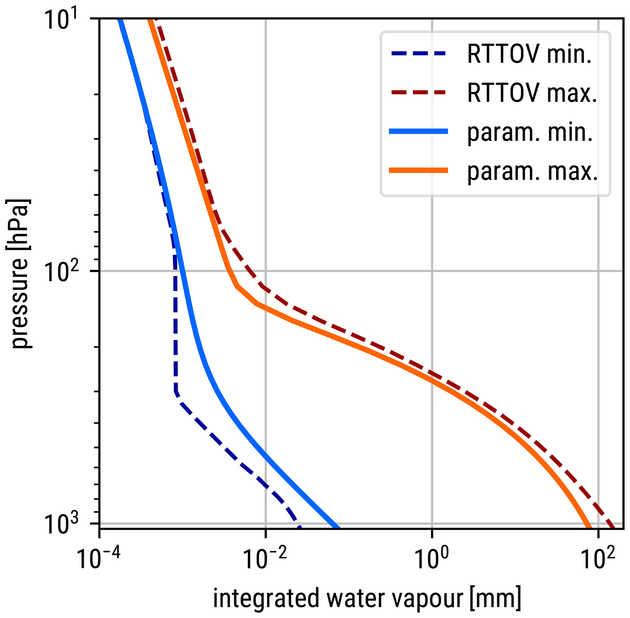
Figure A1 Minimum and maximum integrated water vapour amounts above a given pressure. The dashed lines are integrals over the hard limits in Table 1 of Hocking et al. (2020); the solid lines represent the functions defined in Eqs. (A1) and (A2).

Appendix B: Definition of idealized profiles

The idealized profiles used to compute reflectances from the input parameters are based on the IFS 90-level standard atmosphere, which includes the geometric height $z_i^{\text{IFS}}$, the pressure $p_i^{\text{IFS}}$ and other variables for each level $i=\mathrm{1},\mathrm{\dots },\mathrm{90}$. To construct a grid starting at the desired surface pressure p_sfc, the corresponding height z_sfc is obtained by interpolation in the standard atmosphere. Then a new vertical grid is defined as linear combination ${\stackrel{\mathrm{̃}}{z}}_i=z_i^{\text{IFS}}\times (\mathrm{1}-f_i)+\left(z_{\text{sfc}}+z_i^{\text{IFS}}-z_{\text{sfc}}^{\text{IFS}}\right)\times f_i$ of the original grid and a grid shifted in the vertical such that the lowest level has the correct height. The factor $f_i=\mathrm{1}-{\left(z_i^{\text{IFS}}/z_{\text{sfc}}^{\text{IFS}}\right)}^{\mathrm{2}}$ is chosen such that the original grid is retained for high altitudes and the shifted grid dominates at lower altitudes. For each level the pressure ${\stackrel{\mathrm{̃}}{p}}_i$ corresponding to ${\stackrel{\mathrm{̃}}{z}}_i$ is obtained by linear interpolation in the standard atmosphere. Finally, the level i_ct in $\stackrel{\mathrm{̃}}{p}$ with a pressure closest to the desired cloud top pressure p_ct is identified and the pressure on the five levels $i_{\text{ct}}-\mathrm{2},\mathrm{\cdots },i_{\text{ct}}+\mathrm{2}$ is set to $\left[p_{\text{ct}}-\mathrm{\Delta }p,p_{\text{ct}}-\mathrm{\Delta }p/\mathrm{2},p_{\text{ct}},p_{\text{ct}}+\mathrm{\Delta }p/\mathrm{2},p_{\text{ct}}+\mathrm{\Delta }p\right]$, where $\mathrm{\Delta }p={\stackrel{\mathrm{̃}}{p}}_{i_{\text{ct}}+\mathrm{1}}-{\stackrel{\mathrm{̃}}{p}}_{i_{\text{ct}}}$ to obtain the final pressure grid p_i. Geometric heights z_i corresponding to these pressure levels are again computed by interpolation in the standard atmosphere. The two-layer ice cloud is placed in the two layers above the level i_ct and the two-layer mixed-phase cloud in the two layers below.