The generation of EarthCARE L1 test data sets using atmospheric model data sets

The Earth Cloud, Aerosol and Radiation Explorer mission (EarthCARE) is a multi-instrument cloud–aerosol–radiation process study mission embarking a high spectral resolution lidar, a cloud profiling radar, a multi-spectral imager, and a three-view broadband radiometer. An important aspect of the EarthCARE mission is its focus on instrument synergy. Many L2 products are the result of L1 inputs from one or more instruments. Since no existing complete observational proxy data sets comprised of co-located and co-temporal “EarthCARE-like” data exists, it has been necessary to create synthetic data sets for the testing and development of various retrieval algorithms and the data processing chain. Given the synergistic nature of the processing chain, it is important that the test data are physically consistent across the various instruments. Within the EarthCARE project, a version of the EarthCARE simulator multi-instrument framework (ECSIM) has been used to create unified realistic test data frames. These simulations have been driven using high-resolution atmospheric model data (described in a companion paper). In this paper, the methods used to create the test data scenes are described. In addition, the simulated L1 data corresponding to each scene are presented and discussed.

1 Introduction

The Earth Cloud, Aerosol and Radiation Explorer (EarthCARE; Illingworth et al., 2015) platform comprises a 94 GHz Doppler cloud profiling radar (CPR), 355 nm high spectral resolution atmospheric lidar (ATLID), a multispectral imager (MSI), and a three-view broadband radiometer (BBR). The mission is complex in several aspects. In particular, the synergistic nature of many of the data products and the end-to-end nature of the processing chain (Eisinger et al., 2023; Barker et al., 2023) gives rise to the requirement to generate test data which are realistic and physically consistent from the point of view of all the instruments. For example, combined ATLID, CPR, and MSI measurements will be used within the same synergistic algorithm in order to retrieve, e.g., cloud particle size information. Thus, it is important, from the point of view of the various instruments, that the simulations be conducted in a physically consistent and accurate manner. Crude instrument specific parameterizations (e.g., empirical radar reflectivity vs. cloud ice water content (Z_e vs. IWC) relationships) should be avoided since they are not explicitly related to the basic physical atmospheric properties in a way that can be connected to the other instruments.

The requirement to generate physically consistent simulations with all of the virtual instruments “seeing” the same atmosphere in terms of both macro- and micro-physical considerations was a prime motivation in the original development of the EarthCARE simulator (ECSIM)¹ framework and its component models. ECSIM has been applied to a set of high-resolution cloud-resolving atmospheric model data in order to generate realistic L1 test data sets suitable for EarthCARE algorithm development and testing. Here L1 refers to calibrated and instrument-corrected output generated by the instruments (e.g., lidar-attenuated backscatter, radar reflectivity). L2 data refer to geophysical quantities retrieved using L1 data (e.g., optical extinction, target classification, water content).

The focus of this paper is on the general description of the L1 data sets and how they were generated rather than, e.g., specific algorithm and instrument sensitivity study results. This paper thus serves as a central reference for the several other instrument- and algorithm-specific papers belonging to the EarthCARE level 2 algorithms and data products special issue that rely on the ECSIM-generated L1 test data sets. This paper first presents an overview of the ECSIM. Subsequently, the specific radiative-transfer and instrument simulation methods used for each of the instruments is presented. The paper then concludes with a presentation of the simulated L1 data of the three main EarthCARE testing scenes. The input data used to build these testing scenes are described in a companion paper (Qu et al., 2022).

2 ECSIM overview

ECSIM is not a single model, but rather it is a collection of tools, including radiative-transfer models and instrument models, that cooperate to produce physically consistent simulations covering a range of diverse instruments.

Unlike many common radiative-transfer models, ECSIM is, in principle, not tied to any particular size distribution representation. In particular, multi-wavelength, particle-size-resolved optical and physical characteristics (e.g., mass, maximum dimension, extinction coefficient, and phase function) are stored in a database, while the corresponding bin-resolved size distribution information is specified in separate size distribution files. A separate master scene file stores the 3D fields of temperature, pressure, velocity, and the concentrations of relevant atmospheric gases. This structure allows for the efficient generation of the optical properties necessary to drive diverse forward models. This process is schematically depicted in Fig. 1. In the particular application described in this paper, namely the creation of test frames using Global Environmental Multi-scale (GEM) input fields as a base (Qu et al., 2022) and supplemented by aerosol data from Copernicus Atmosphere Monitoring Service (CAMS) reanalysis fields (Inness et al., 2019), the GEM and CAMS data were translated into ECSIM scene files using purpose built computer programs.

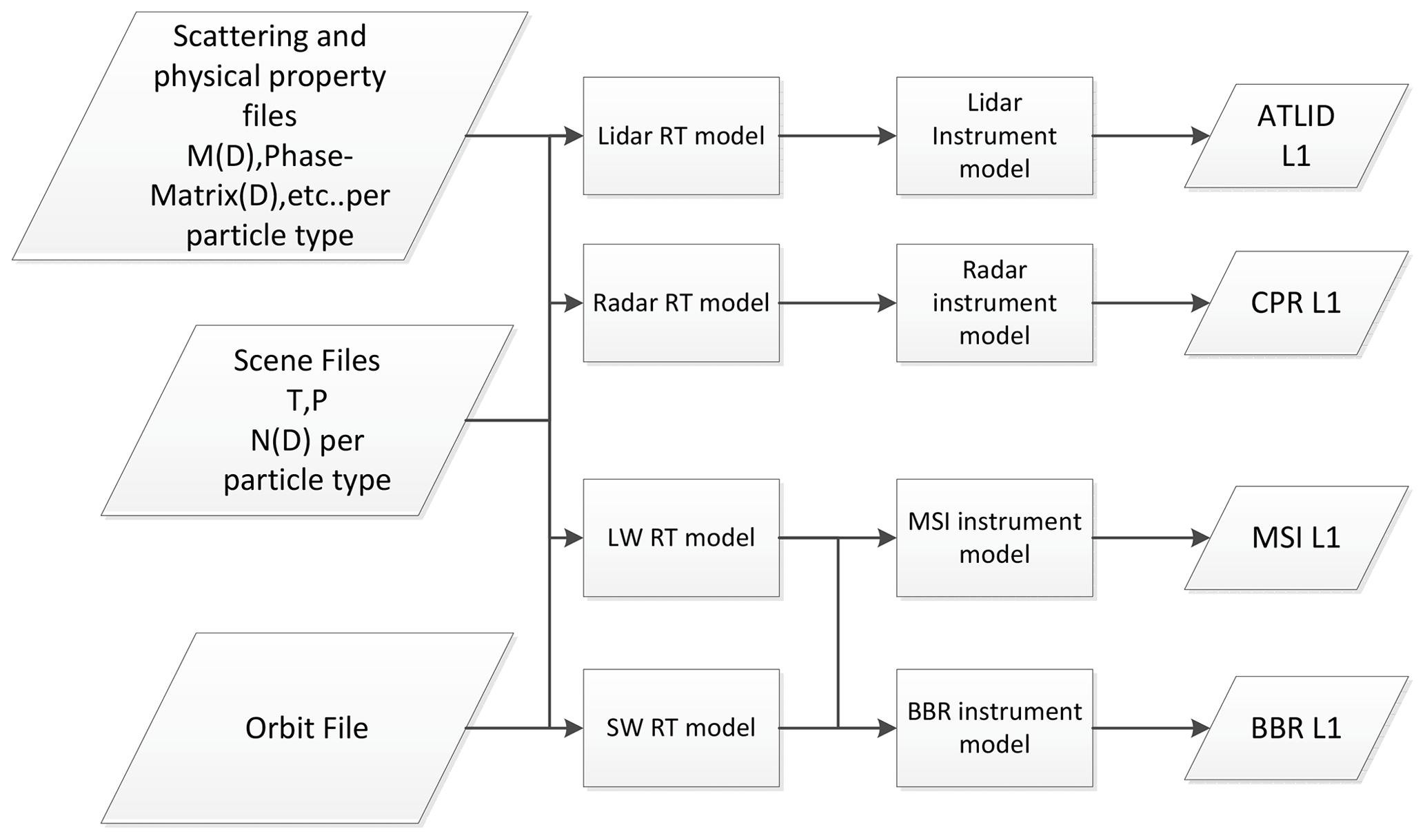
Figure 1 High-level structure of ECSIM. All of the radiative-transfer models read the same scene information. Another feature is that the radiative-transfer models are separate from the instrument simulation models.

A key aspects of the ECSIM structure is that all the instrument simulations are driven by the same unambiguously defined atmosphere. All of the individual radiative-transfer models read the same scene files and access the same scattering information data files. Whenever a model needs to calculate, for example, cloud extinction at a required wavelength, the appropriate binned size distribution (read from the scene files) is combined with the appropriate scattering properties (read from the scattering library). This structure facilitates the production of physically consistent simulations; i.e., it helps ensure that the radiative-transfer models all “see the same atmospheric particles” and are “discouraged” from making their own ad hoc assumptions regarding particle size distributions or optical and physical properties (e.g., different mass–maximum dimension relationships for ice cloud particles).

2.1 Representation of the scene constituents

2.1.1 Hydrometeor microphysical properties

The Global Environmental Multi-scale (GEM) Numerical Weather Prediction (NWP) models runs for the EarthCARE algorithm development efforts (Qu et al., 2022) supports six different hydrometeor types: cloud droplets, raindrops, ice, snow, graupel, and hail using a bin microphysical representation. The model bin warm microphysics scheme represents the cloud droplets particle size distribution in 50 bin sizes centered at values corresponding to cloud droplet diameters from 2 to 100 µm and the rain particle size distribution in 50 bin sizes centered at values corresponding to raindrop radius from 50 to 2500 µm. The Environment and Climate Change Canada (ECCC) cold microphysics scheme used by GEM supports four different types of particles: cloud ice, snow, graupel, and hail. The particle size distribution of cloud ice is represented in 50 bin sizes centered at values corresponding to ice particle radius from 2 to 100 µm every 2 µm. The particle size distributions of snow is represented by 100 bin sizes each from 25 to 2500 µm every 10 µm. Table 1 summarizes the details of the bin representation of the hydrometeor species in GEM. When translating the GEM cloud information to ECSIM, certain adjustments were made to the cold cloud microphysics. As detailed in Qu et al. (2022) these adjustments improved the realism of the simulations. Accordingly, the ECSIM ice and snow hydrometeors categories have particle mass (M) and cross-sectional area (A_c) according to the Erfani and Mitchell (2016) relations for synoptic cirrus and temperatures between −40 and −20 ^∘C. The mass of the ice and snow particles in grams is given by the expression $M\left(D\right)=\exp \left[a_{\mathrm{0}}+a_{\mathrm{1}}\ln \left(D\right)+a_{\mathrm{2}}\left[\ln \right(D){]}^{\mathrm{2}}\right]$, where D is in centimeters and the coefficients have values of $a_{\mathrm{0}}=-\mathrm{6.72924}$, a₁=1.17421, and $a_{\mathrm{2}}=-\mathrm{0.15980}$.

Erfani and Mitchell (2016)Erfani and Mitchell (2016)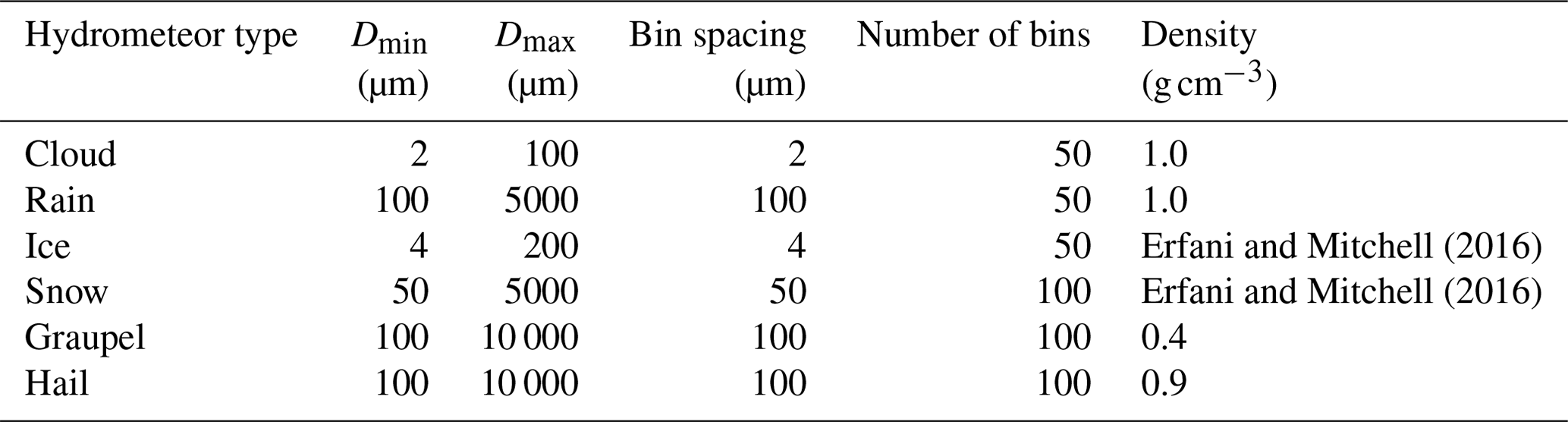

Table 1 GEM Cloud and precipitation microphysical parameters.

2.1.2 VIS-UV-IR hydrometer optical properties

In ECSIM, the optical scattering properties of cloud droplets and raindrops for visible (VIS), ultra-violet (UV), and infrared (IR) wavelengths are all calculated using Mie theory. The optical scattering and absorption properties of each bin are determined by averaging the scattering and absorption properties over 20 equally spaced sub-bins. Temperature-dependent refractive indices were used (Hale and Querry, 1973) and calculations were done for temperatures of 240 and 300 K and optical information at specific temperatures was found via interpolation.

For the GEM scenes, the UV-IR extinction, absorption, and phase functions for ice and snow were adapted from Baum et al. (2014) using the single-particle effective radius to interpolate in particle size. Here, the effective radius is defined as

$$\begin{array}{}\text{(1)}& R_{\mathrm{eff}}\left(D\right)={\displaystyle \frac{\mathrm{3}M\left(D\right)}{\mathrm{4}{\mathit{\rho }}_{\mathrm{i}}{A}_{\mathrm{c}}\left(D\right)}},\end{array}$$

where D is the particle maximum dimension, M(D) is the particle mass, A_c(D) is the cross-sectional area of the particle, and ρ_i is the density of solid ice. The M(D) and A_c(D) relationships used are listed in Table 1 and are described in more detail in Qu et al. (2022).

For both cloud ice and snow particle types, the Baum Aggregated Solid Columns properties were used. For cloud ice, particle maximum dimensions between 4 and 200 µm were used in steps of 4 µm. For snow, sizes between 50 and 5000 µm in steps of 25 µm were used. The aggregated solid-column phase functions generally do not have strong halo features, which is in accordance with observations (Baum et al., 2014). The aggregated solid-column phase functions also lack a backscatter peak; however, this is likely not in accordance with observations. In particular, in Zhou and Yang (2015), the backscatter issue was investigated. They found that by directly solving Maxwell's equations numerically, a narrow backscattering peak was present for a wide range of types of ice crystals (i.e., irregular smoothed, smoothed, roughened hexagons). The width of the backscatter peak is inversely proportional to the size parameter. They also showed that accounting for this peak produces more realistic values of the lidar ratio and improves the agreement between lidar multiple-scattering coefficients derived using CALIPSO observations and theory (Zhou and Yang, 2015). Accordingly, for the lidar specific radiative-transfer calculations (Sect. 2.2) a backscatter peak was added to the ice-phase function following the procedure described in Zhou and Yang (2015).

For graupel and hail, for the UV-IR optical properties Mie calculations were applied to equivalent effective radius spheres. This procedure produces reasonably accurate estimates of the extinction and absorption (Grenfell and Warren, 1999); however, the phase functions will not be accurate. This was not considered to be an important issue as, in the scenes considered here, occurrences of these scattering types are masked by significant amounts of cloud ice and/or snow when viewed from above.

2.1.3 Microwave scattering and absorption

Mie scattering is used for the estimation of the backscattering and extinction coefficients for cloud droplets and raindrops. For ice and snow, the self-similar Rayleigh–Gans approximation (Hogan et al., 2017) is used for modeling of backscattering properties of ice and snow. The particles are assumed to be horizontally aligned with an aspect ratio of 0.6. The parameters for aggregates of bullet rosettes are as in (Hogan and Westbrook, 2014). Graupel and hail are modeled as the equal-mass spheres consisting of a blend of ice and air and using Mie theory. The dielectric properties of the mixture are calculated using Maxwell–Garnett approximation and assuming the ice inclusions in an air matrix. The gaseous attenuation is estimated using the Rosenkranz's method (Rosenkranz, 1998). The raindrops terminal velocity is estimated using Brandes et al. (2002) and the ice and snow particle fall velocity is based on Mitchell and Heymsfield (2005).

2.1.4 Aerosol microphysical and optical properties

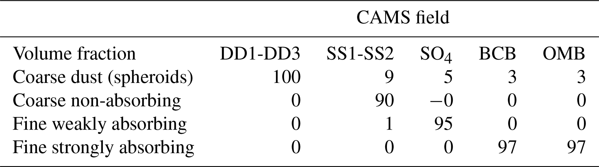
The aerosol fields were constructed using CAMS aerosol component fields mapped to the following “Hybrid End-To-End Aerosol Classification” (HETEAC) (Wandinger et al., 2022) base component types following Table 2; more detail is given in Qu et al. (2022). We reiterate here that goal of this exercise is not to produce an “optimally accurate” mapping. An ad hoc approximate approach in order to produce a range of “realistic enough” aerosol conditions with different optical characteristics was sufficient for the goals of the work presented here.

Table 2 Mapping between CAMS aerosol components and HETEAC aerosol component types. The CAMS fields used are desert dust (DD) size ranges 1 to 3, sea salt (SS) sizes ranges 1 and 2, sulfate (SO₄), hydrophilic black carbon (BCB), and hydrophilic organic matter (OMB).

2.1.5 Optical gaseous absorption

The ECSIM scenes contain the following (limited) number of gaseous species: O₂, N₂, CO₂, H₂O, O₃.

For the MSI and BBR simulations, the atmospheric transmission is calculated using a correlated-k method (Kato et al., 1999) for various narrow bands. For each narrow band, the aerosol and cloud optical properties are treated as being constant and represent a simple average across the band.

2.1.6 Shortwave surface radiative properties

For the shortwave water surfaces, the azimuth-dependent bi-directional reflectance distribution function (BRDF) for the GEM derived scenes were calculated as a function of wind speed based on lookup tables derived from the matrix operator model (MOMO) radiative-transfer model (Hollstein and Fischer, 2012) (run in unpolarized mode). The MOMO ocean BRDFs (Fell and Fischer, 2001) themselves are based on a Cox–Munk approach.

For the non-snow and ice SW land surfaces, the isometric–volumetric–geometric (Iso-Vol-Geo) kernel-based approach is used (Schaaf et al., 2002). For the GEM scenes, Iso-Vol-Geo coefficients for non-ice and snow areas for a number of specific bands were supplied. The BRDFs at these bands then served as inputs to a principal-component-based procedure for generating BRDFs for general SW frequencies (Vidot and Borbáas, 2014). For ice and snow surfaces, the surfaces were treated as being Lambertian with the albedo being assigned by underlying surface type (taken from the GEM model) following Moody et al. (2007).

2.1.7 Longwave surface radiative properties

For the longwave radiative-transfer calculations a much simpler approach was used. The surfaces were treated as being Lambertian, and the emissivity was assumed to be a constant value of 0.93 over water and 0.98 over land.

2.2 Lidar radiative-transfer calculations

The lidar simulation is separated into two main steps. First a lidar-specific radiative-transfer model is used to calculate the time-spectral-polarization-resolved lidar backscatter. Then a separate instrument model is applied to the output of the lidar radiative-transfer model to simulate the effect of, e.g., instrument noise and non-ideal spectral filtering. The lidar radiative-transfer methods are described in this section, and the lidar instrument model is then described in Sect. 2.3.

2.2.1 Basic considerations

For a single-wavelength non-polarized lidar, the single-scattered power incident upon the detection element for a completely elastic backscatter lidar (neglecting the background signal) for an appropriate wavelength interval centered around λ_l can be written as

$$\begin{array}{}\text{(2)}& P(z,{\mathit{\lambda }}_{\mathrm{l}})=C_{\mathrm{lid}}{z}^{-\mathrm{2}}{\mathit{\beta }}_{\mathit{\pi }}(z,{\mathit{\lambda }}_{\mathrm{l}})\exp \left[-\mathrm{2}\underset{\mathrm{0}}{\overset{z}{\int }}\mathit{\alpha }\left(z^{\prime },{\mathit{\lambda }}_{\mathrm{l}}\right)\mathrm{d}{z}^{\prime }\right],\end{array}$$

where λ_l is the laser wavelength, P(z,λ_l) is the power the lidar will receive from a target a distance $z=ct/\mathrm{2}$ from the lidar (where t is the elapsed time since the laser pulse was launched from the lidar), β_π(z,λ_l) is the range- and wavelength-dependent backscatter coefficient, and $\mathit{\alpha }(z^{\prime },{\mathit{\lambda }}_{\mathrm{l}})$ is the extinction coefficient. Here both the backscatter and extinction coefficients represent appropriate averages over the wavelength interval of interest. C_lid is a constant that takes into account factors related to the lidar's physical characteristics.

$$\begin{array}{}\text{(3)}& C_{\mathrm{lid}}=T_{\mathrm{r}}{E}_{\mathrm{l}}{A}_o,\end{array}$$

where T_r is the bulk effective receiver transmission, E_l is the laser pulse energy, and A_o is the effective receiver area.

2.2.2 Multiple scattering

Equation (2) is valid only when single scattering is predominant. In cases where either a high proportion of scattered photons remain within the receiver field of view (FOV) or the optical depth is such that photon mean free path is small compared to the instantaneous sampling volume then multiple scattering (MS) effects must be taken into account. In general, these conditions are often met for ground-based remote sensing of clouds and are always met for the case of space-based cloud remote sensing.

In order to account for multiple scattering, the lidar radiative-transfer simulations were conducted using the ECSIM-3D lidar Monte Carlo radiative transfer code. The approach used is described within (Donovan et al., 2015), and additional relevant detail not covered within Donovan et al. (2015) is given here. In particular, the approach used to determine the spectral properties of the return signal is discussed. Within the MS model, each photon packet is assigned both a mean relative spectral shift (initially zero) from its center wavelengths and a Gaussian spectral width. The Doppler shift in the packets is calculated according to the relative velocity of the scatterers encountered and the scattering geometry. The spectral width is initialized using the laser line width and is hardly affected by particulate scattering but can be substantially widened if molecular scattering has occurred.

2.2.3 Doppler shift and multiple scattering

Even neglecting such processes involving the change in energy levels within the target scatterers (i.e., rotational–vibrational Raman scattering, fluorescence) the scattered radiation will be Doppler-shifted according to the relative motion of the scatterers with respect to the lidar. In general, a target moving with respect to a fixed lidar will “see” a source whose frequency is given by (neglecting terms of order ${\left(v/c\right)}^{\mathrm{2}}$)

$$\begin{array}{}\text{(4)}& f=f_o\left(\mathrm{1}+{\displaystyle \frac{v}{c}}\cos \left(\mathit{\theta }\right)\right),\end{array}$$

where v is the velocity of the scatterer, c is the speed of light, θ is the angle between the scatterers velocity vector and the line-of-sight directed back toward the receiver, and f_o is the frequency of the source light in the frame of the laser. When light initially incident upon the moving scatterer, is scattered, it is equivalent to being instantaneously absorbed and re-emitted so that the scattered light will again be Doppler shifted in frequency depending on the motion of the scatterer with respect to the receiver. Accordingly, the frequency measured by an observer in the same frame as the lidar transmitter will be given by (again neglecting terms of order ${\left(v/c\right)}^{\mathrm{2}}$)

$$\begin{array}{}\text{(5)}& f=f_o\left[\mathrm{1}+{\displaystyle \frac{v}{c}}\left(\cos \left(\mathit{\theta }\right)+\cos \left({\mathit{\theta }}_{\mathrm{sc}}\right)\right)\right],\end{array}$$

where θ_sc is the angle between the velocity vector and the scattered photon's trajectory. This means that light scattered directly forward and measured by a stationary observer would have no Doppler shift while light scattered directly backwards to the lidar would be observed to have been shifted in wavelength by an amount twice that predicted by Eq. (4).

The occurrence of multiple scattering will have implications with respect to the spectral signature of the lidar return. By repeated application of Eq. (4) (see Fig. 2) it can be shown that the Doppler-shifted frequency after n scatters as measured by an observer in the same frame of reference as the lidar will be given by

$$\begin{array}{}\text{(6)}& \begin{array}{rl}{f}_n=& f_o(\mathrm{1}+{\displaystyle \frac{\mathrm{1}}{c}}({\mathit{v}}_{\mathrm{1}}\cdot {\mathit{I}}_{\mathrm{0}}+({\mathit{v}}_{\mathrm{1}}-{\mathit{v}}_{\mathrm{2}})\cdot {\mathit{I}}_{\mathrm{1}}\\ & +({\mathit{v}}_{\mathrm{2}}-{\mathit{v}}_{\mathrm{3}})\cdot {\mathit{I}}_{\mathrm{2}}+\mathrm{\cdots }{\mathit{v}}_n\cdot {\mathit{I}}_n\left)\right),\end{array}\end{array}$$

where v_i is the velocity vector of the ith scatterer and I_i is the unit vector for the photon trajectory for the ith scatter. If the lidar is to observe the photon to a good approximation, it must be scattered directly backwards towards the lidar receiver so that ${\mathit{I}}_n=-{\mathit{I}}_{\mathrm{0}}$ and thus

$$\begin{array}{}\text{(7)}& \begin{array}{rl}{f}_n=& f_o(\mathrm{1}+{\displaystyle \frac{\mathrm{1}}{c}}({\mathit{v}}_{\mathrm{1}}\cdot {\mathit{I}}_{\mathrm{0}}+({\mathit{v}}_{\mathrm{1}}-{\mathit{v}}_{\mathrm{2}})\cdot {\mathit{I}}_{\mathrm{1}}+\\ & ({\mathit{v}}_{\mathrm{2}}-{\mathit{v}}_{\mathrm{3}})\cdot {\mathit{I}}_{\mathrm{2}}+\mathrm{\cdots }-{\mathit{v}}_n\cdot {\mathit{I}}_{\mathrm{0}}\left)\right)\end{array}.\end{array}$$

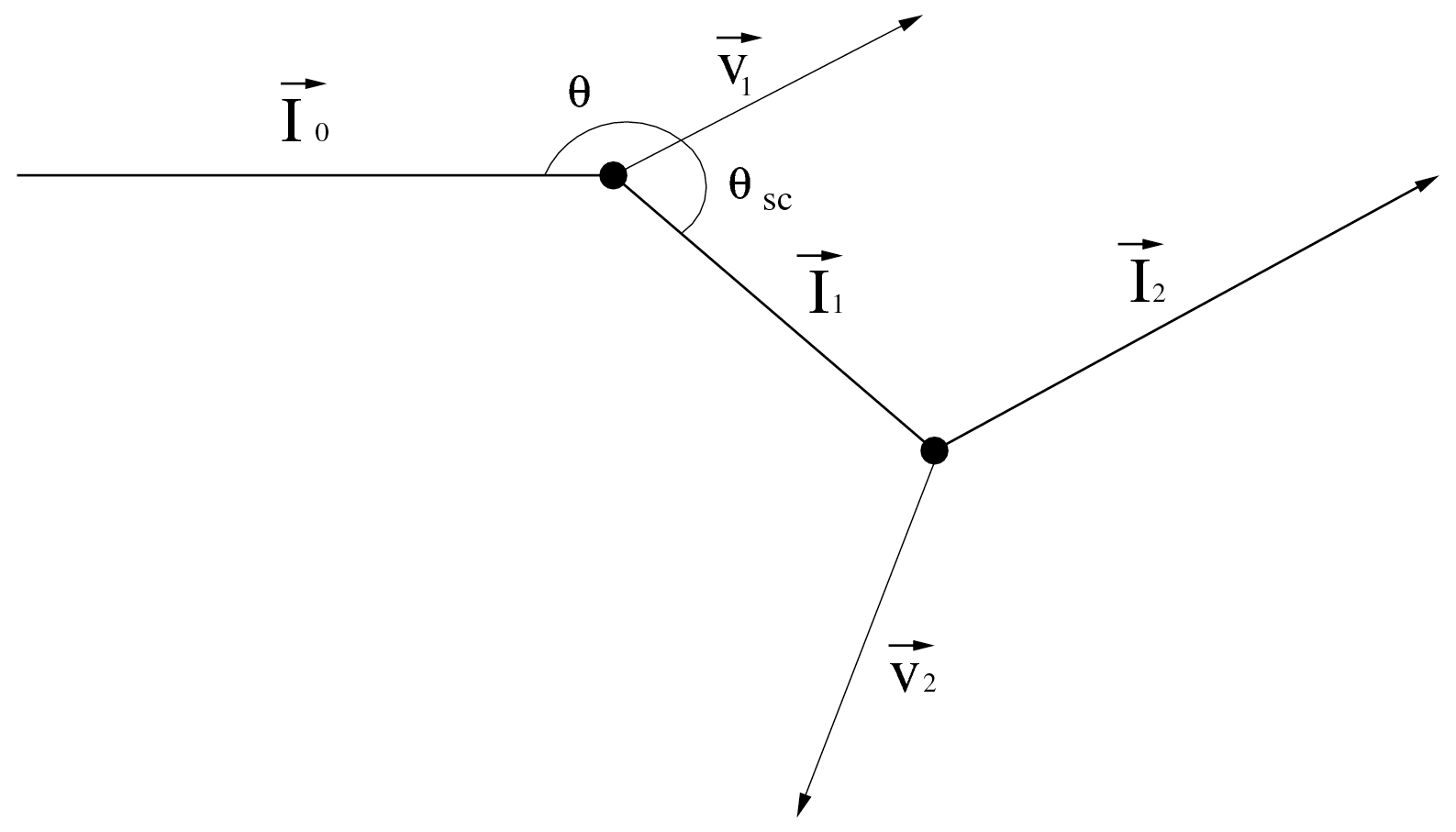
Figure 2 Geometry relevant for determining the observed Doppler shift after multiple scatters.

2.2.4 Spectral broadening and multiple scattering

In the MC model the spectral width of the packets is also tracked. The width is initialized using the laser spectral line width. The Gaussian width after subsequent scattering events is calculated by convolving the spectral width of the incoming packet with the spectral width induced by the scattering event (accounting the scattering geometry). For particulate scattering, the spectral width is assumed to be unaffected. However, for molecular scattering events thermal broadening is important. How this is modeled in ECSIM is described in the following subsection.

A schematic representation of the spectral signature of a general lidar return signal is shown in Fig. 3. The spectral width of the particulate backscattering peak will be determined by the spectral width of the laser pulse itself along with any turbulence present in the sampling volume. The spectral width of the laser will be on the order of 10⁻⁷f_o, so that the laser line width will usually be the dominant factor. The molecular backscatter though, will be much spectrally broader than the particulate scattering return; this is due to the fact that the atmospheric molecules have a large thermal velocity. For low densities the half-maximum half width (HMHW) of the broadening produced by the thermal motions alone is given by

$$\begin{array}{}\text{(8)}& \mathrm{\Delta }f=f_o\left({\displaystyle \frac{\mathrm{8}kT\log \left(\mathrm{2}\right)}{M{c}^{\mathrm{2}}}}\right),\end{array}$$

where k is Boltzmann's constant, M is the average molecular mass, and T is temperature. For typical values of atmospheric temperature, the HMHW of the Doppler return will be on the order of $\mathrm{4}\times {\mathrm{10}}^{-\mathrm{6}}{f}_o$ so that the Doppler broadening will be 10–20 greater than the laser line width. Equation (8) applies at low gas densities.

Figure 3 Idealized view of spectral signature of a lidar return.

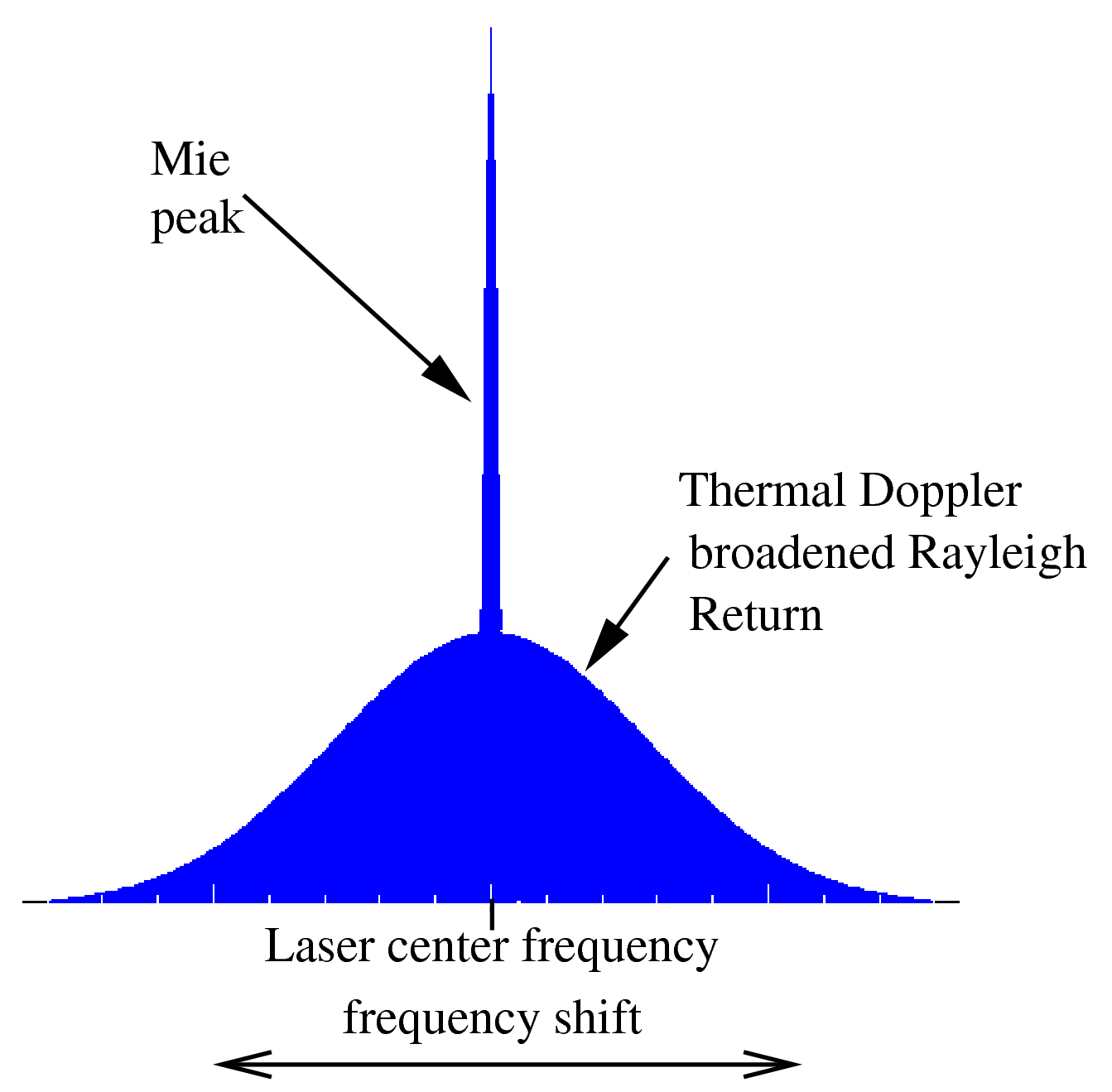
In general, the central (non-Raman) Rayleigh line profile (Cabannes line) will consist of three components, a central peak together with two flanking “Brillouin–Mandel'shtam” peaks (Miles et al., 2001). In the low-density or high-temperature regimes the uncorrelated motion of the scatterers gives rise to a Gaussian velocity distribution centered around the mean velocity of the flow and Eq. (8) applies. As the pressure increases or the temperature decreases, density fluctuations on the order of the laser wavelength will appear. These density fluctuations travel at the speed of sound in the gas and will give rise to acoustic side bands.

The Rayleigh–Brillouin scattering line shape may be quantified in terms of the so-called y parameter, which is defined in terms of the ratio of the laser wavelength to the mean free path. For the Earth's atmosphere

$$\begin{array}{}\text{(9)}& y=\mathrm{0.230}\left[{\displaystyle \frac{T+\mathrm{111}}{T^{\mathrm{2}}}}\right]\left[{\displaystyle \frac{P\mathit{\lambda }}{\sin \left(\frac{\mathit{\theta }}{\mathrm{2}}\right)}}\right],\end{array}$$

where T is the temperature in Kelvin, P is the pressure in atmospheres, λ is the laser wavelength in nanometers, and θ is the scattering angle. Here x is a normalized frequency parameter defined as

$$\begin{array}{}\text{(10)}& x={\displaystyle \frac{\sqrt{\mathrm{2}}\mathit{\lambda }}{\mathrm{4}\sin \left(\frac{\mathit{\theta }}{\mathrm{2}}\right)}}\left({\displaystyle \frac{\mathit{\nu }}{{\mathit{\nu }}_o}}\right),\end{array}$$

where ν is the frequency shift from the line center and ν_o is the sound speed

$$\begin{array}{}\text{(11)}& {\mathit{\nu }}_o=\sqrt{{\displaystyle \frac{kT}{m}}},\end{array}$$

where m is the molecular mass.

For low y parameters, the line shape has a simple Gaussian form. For larger values of y (in the range that we must be concerned with) the line shape becomes complicated and somewhat costly to evaluate. Fortunately, for values of y under about 10, the Rayleigh–Brillouin line shape may be accurately approximated by the sum of three independent Gaussian functions (Witschas, 2011).

For the single-scatter return the line shape is determined by the sum of three Gaussian profiles. These calculations are based on the results of pre-computed approximate Gaussian fits made to accurate calculations of the line profile (Pan et al., 2002) corresponding to various y parameters (see Fig. 4). For the higher-order scattering, at each molecular scattering event the probability of the scattered photon packet being shifted to one of the acoustic side bands is calculated. Whether or not the center frequency of the photon packet is shifted is then determined stochastically using the relative weights of the component Gaussians, and the subsequent shift and width of the associated Gaussian profile is used to determine the line shape. This line shape and shift is then used subsequently for the next multiple-scattering event.

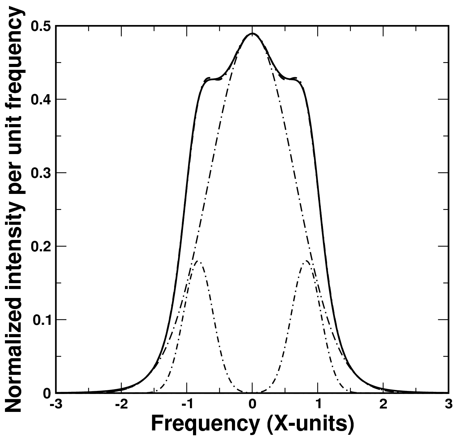
Figure 4 Exact Rayleigh–Brillouin line shape (solid line) along with fitted sum of three Gaussian functions (dashed–dotted line). The three-component Gaussian functions are also shown. Here the y parameter is equal to 1.0.

2.3 Lidar instrument model

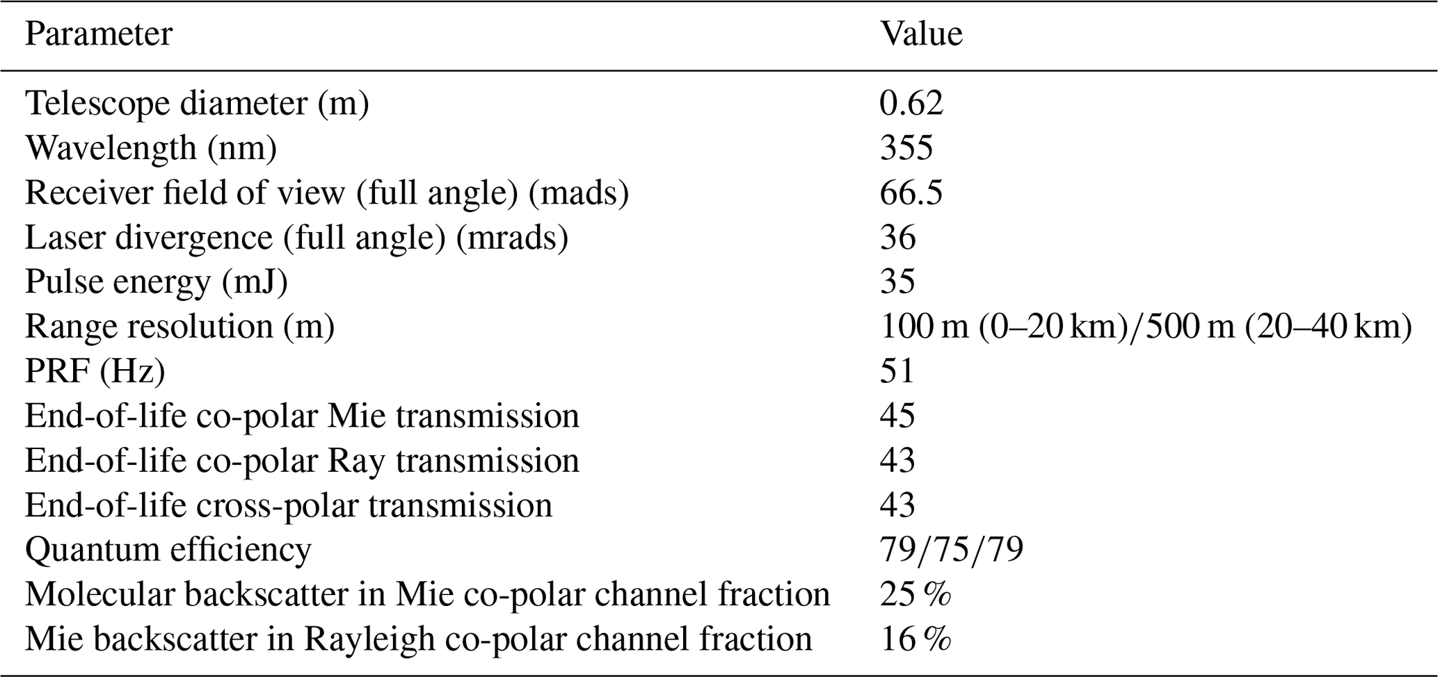
ATLID transmits a linearly polarized beam and possesses three receiver channels. A co-polar “Mie” channel which detects mainly particulate (i.e.,  clouds and aerosol) backscatter, a co-polar “Rayleigh” channel which detects mainly backscatter from molecules, and a cross-polar particulate+molecular channel. The Mie-Rayleigh separation is achieved using a Fabry–Pérot etalon. For details of ATLID's design, see do Carmo et al. (2016) and do Carmo et al. (2021). Some of the important ATLID technical specifications are repeated in Table 3.

Table 3 ATLID technical specifications.

The ECSIM lidar instrument model ingests the output of the lidar radiative transfer model and models the instrument response function including instrument noise. The model is capable of being configured to simulate various lidars, in this case ATLID. The instrument model ingests the time-spectral-polarization-resolved output of the lidar radiative transfer model and models the three different optical ATLID detection channels. Explicit modeling of the Fabry–Pérot etalon high-spectral resolution lidar (HSRL) spectrometer and various other optical elements in each detector path are performed. The effects of Poisson shot noise on the simulated observed signals is simulated. Instrument dark current and solar background effects are taken into account. Since ATLID's detector elements are accumulation charge-coupled devices (ACCDs) they are subject to read-out noise. The effects of this read-out noise are also simulated.

2.3.1 Background signal

The background signal refers to power registered by the lidar receiver that is due to the detection of photons from sources other than backscattered laser light. In the case here, the main source of background light will be scattered sunlight from the Earth's surface and atmosphere. As such, the background will depend on the solar angle, the surface type, and the cloud cover. In this work, the lidar background values were based on an approximate lookup table approach where the background irradiance at 355 nm was modeled using a radiative model for various cloud optical depths, surface albedos, and solar zenith angles.

The background power incident upon the detector level is given by

$$\begin{array}{}\text{(12)}& P_{\mathrm{back}}=A_o\mathit{\pi }{\mathit{\rho }}_{\mathrm{t}}\stackrel{\mathrm{‾}}{I_b\left(\mathit{\lambda }\right)T_{\mathrm{rec}}\left(\mathit{\lambda }\right)}\mathrm{\Delta }\mathit{\lambda },\end{array}$$

where A_o is the effective receiver area, ρ_t is the telescope 0.5 angle field of view, $\stackrel{\mathrm{‾}}{I_b\left(\mathit{\lambda }\right)T_{\mathrm{rec}}\left(\mathit{\lambda }\right)}$ is the average product of the receiver-wavelength-dependent transmission (including filtering) with the upwelling irradiance, and Δλ is the wavelength interval that must be considered.

2.3.2 Receiver optical elements

The ATLID lidar receiver optical train is modeled as a sequence of elements (beam splitters, spectral filters, half-wave plates, etc.) that operate on the spectral and polarization state of the lidar return. For simplicity, broadband spectral filters are modeled as having a rectangular passbands and are characterized by a single in-band transmission and reflection and an out-of-band reflection and transmission pair.

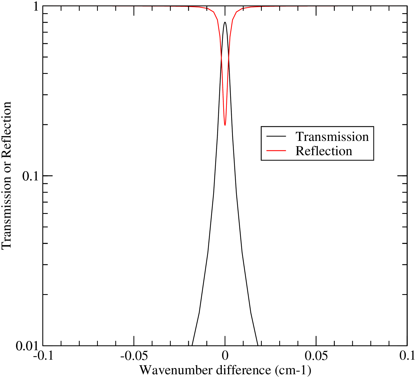
The Fabry–Pérot (FP) etalon is the most critical optical element in ATLID's receiver chain. This element is used to separate the Mie signal from the Rayleigh signal.

The transmission function of an etalon without accounting for non-ideal effects such as the finite input beam collimation and surface roughness may be modeled (Saleh and Teich, 1991) as

$$\begin{array}{}\text{(13)}& T=\left(\mathrm{1}-{\displaystyle \frac{A}{\mathrm{1}-R}}\right)\times {\displaystyle \frac{\mathrm{1}}{\mathrm{1}+\frac{\mathrm{4}R}{(\mathrm{1}-R{)}^{\mathrm{2}}}{\sin }^{\mathrm{2}}\frac{\mathit{\delta }}{\mathrm{2}}}},\end{array}$$

where R is the reflection coefficient of the etalon mirrors, A is the relative absorption and scattering loss parameter, and $\mathit{\delta }=\mathrm{2}\mathit{\pi }\frac{\mathit{\lambda }-{\mathit{\lambda }}_o}{{\mathit{\lambda }}_o}$, where λ_o is the central wavelength. The corresponding etalon reflection function (R_fp) may be written as follows:

$$\begin{array}{}\text{(14)}& R_{\mathrm{fp}}={\displaystyle \frac{{\left(\mathrm{1.0}-R-A\right)}^{\mathrm{2}}}{\mathrm{1.0}-\mathrm{2.0}\times R\cos \left(\mathit{\delta }\right)+R^{\mathrm{2}}}}.\end{array}$$

The effects of non-parallel mirror flatness, diffraction, and non-ideal beam collimation are taken into account by convolving the above absorbing etalon transmission and reflection functions by a top-hat function whose width in wavenumbers is given by

$$\begin{array}{}\text{(15)}& \mathrm{\Delta }{\mathit{\nu }}_{\mathrm{total}}=\sqrt{\mathrm{\Delta }{\mathit{\nu }}_{\mathrm{np}}^{\mathrm{2}}+\mathrm{\Delta }{\mathit{\nu }}_{\mathrm{ap}}^{\mathrm{2}}+\mathrm{\Delta }{\mathit{\nu }}_{\mathrm{dif}}^{\mathrm{2}}},\end{array}$$

where Δν_np accounts for the broadening due to non-parallel mirror alignment, Δν_ap accounts for collimation or finite aperture effects

$$\begin{array}{}\text{(16)}& \mathrm{\Delta }{\mathit{\nu }}_{\mathrm{ap}}=\mathrm{1.0}-\cos \left[{\left({\displaystyle \frac{D_{\mathrm{t}}}{D_{\mathrm{fp}}}}\right)}^{\mathrm{2}}{\displaystyle \frac{{\mathit{\rho }}_{\mathrm{t}}}{\mathrm{2}}}\right],\end{array}$$

where D_t is the telescope diameter, D_fp is the etalon diameter, and ρ_t is the telescope full-angle field of view in radians. Δν_dif accounts for diffraction effects and is given by

$$\begin{array}{}\text{(17)}& \mathrm{\Delta }{\mathit{\nu }}_{\mathrm{dif}}=\mathrm{1.0}-\cos \left[\left({\displaystyle \frac{{\mathit{\lambda }}_o}{D_{\mathrm{t}}}}\right)\right].\end{array}$$

An example etalon transmission and reflection profile as a function of ν−ν_o is shown in Fig. 5. Here T=0.978, A=0.0, the free spectral range (the distance between adjacent transmission maximums) is 0.5 cm⁻¹, the flatness parameter is ${\mathit{\lambda }}_o/\mathrm{300}$, the telescope field of view (FOV) is $\mathrm{5}\times {\mathrm{10}}^{-\mathrm{3}}$ mrad, the telescope diameter is 0.6 m, and the etalon diameter is 0.05 m.

Figure 5 Etalon reflection and transmission showing non-ideal behavior.

2.3.3 Noise considerations

For a given time interval, the number of photons arriving at a given detector channel is given by

$$\begin{array}{}\text{(18)}& N_{\det }=R_{\det }{\displaystyle \frac{{\mathit{\lambda }}_o}{hc}}\left(P_{\mathrm{lid}}+P_{\mathrm{back}}\right)\mathrm{\Delta }t,\end{array}$$

where Δt is the averaging time interval, h is Planck's constant, λ_o is an appropriate mean wavelength for the detector channel in question, R_det is the detector quantum efficiency, P_lid is the power received at the lidar detector, and P_back is the background power arising from the upwelling reflected solar radiance at 355 nm. According to Poisson statistics, the standard deviation of N_det, shot noise, is simply given by

$$\begin{array}{}\text{(19)}& \mathit{\delta }{N}_{\det }=\sqrt{N_{\det }}.\end{array}$$

In addition to the shot noise, the effects of dark current noise and ACCD readout noise are also simulated. The average dark current is a characteristic of the detection electronic chain, and its mean level is assumed to be constant in terms of effective noise photocounts per unit time. The dark-count rate is assumed to follow Poisson statistics. The read-out noise is a characteristic of CCD detectors and is applied only at simulated read-out time. For ATLID, the envisioned default mode is for the ACCD to accumulate two shots before read-out. The mean read-out noise is assumed to be constant per read-out event and is modeled using Poisson statistics.

2.3.4 Spectral and polarization cross-talk

The characteristics of the HSRL filter ensure that a degree of spectral cross-talk between the Mie and Rayleigh channels exists (do Carmo et al., 2021). The effects of cross-talk are simulated within the lidar instrument model. The lidar instrument model also applies a cross-talk correction, following the ATLID L0 to L1 processor step. This correction assumes perfect knowledge of the appropriate cross-talk coefficients. In flight, uncertainties in the coefficients will introduce additional errors; however, this is not envisioned to be a significant issue as the in-flight values of the coefficients are envisioned to be known within an accuracy of a few percent. This is to be achieved using a combination of a priori on-ground characterization and in-flight monitoring and adjustment, e.g., using returns above 30 km (where only molecular scattering returns should be expected) to quantify the amount of Rayleigh-to-Mie cross-talk and using ground and suitably strong cloud returns (where to a good approximation only elastic particulate scattering returns exist) to quantify the Mie-to-Rayleigh cross-talk. Due to the occurrence of variable but significant amounts of molecular Brillouin scattering in liquid water (Hostetler et al., 2018), water surfaces are not expected to be suitable cross-talk coefficient determination targets for ATLID.

For simplicity, the simulations presented in this paper did not consider polarization cross-talk. However, as is the case with lidars in general, due to non-ideal optical element characteristics, laser polarization purity, and imperfect optical element orientation and alignments, a degree of polarization cross-talk will be present in the ATLID instrument (Bravo-Aranda et al., 2016; Donovan et al., 2015). The correction of spectral cross-talk effects will be conducted at the L1 stage by the L0 to L1 processor. The estimated errors will be reported in the L1 product.

The characterization of the ATLID polarization cross-talk has been the subject of extensive ground testing and characterization, e.g., do Carmo et al. (2016). For example, in-flight characterization and monitoring of the spectral cross-talk is planned to be accomplished using high-altitude returns where the Rayleigh depolarization signal is known and from solar background measurements over thick ice clouds at high sun conditions.

2.4 Radar simulation

2.4.1 Radar radiative transfer calculations

The radar scattering calculations described in Sect. 2.1.3 are used to estimate the radar backscatter cross-section σ_b,j(D) for each hydrometeor species j and particle maximum diameter D in units of m². In addition, the extinction cross-section σ_e,j(D) for each hydrometeor species j and particle maximum diameter D is estimated in units of m². The GEM particle size distribution number concentration n_j(D) is provided in units of m⁻³ (integrated across the bin diameter width) and the particle sedimentation velocity V_j(D) is provided in units of m s⁻¹.

Thus, the radar reflectivity factor Z_e (mm⁶ m⁻³), specific attenuation A (dB km⁻¹) and reflectivity-weighted hydrometeor sedimentation velocity V_SED (m s⁻¹) are estimated for each hydrometeor species as follows:

$$\begin{array}{}\text{(20)}& Z_{\mathrm{e},j}={\mathrm{10}}^{\mathrm{18}}{\displaystyle \frac{{\mathit{\lambda }}^{\mathrm{4}}}{{\mathit{\pi }}^{\mathrm{5}}\left|K_{\mathrm{w}}^{\mathrm{2}}\right|}}\sum _{i=\mathrm{1}}^{\mathrm{Nbins}}\left[{\mathit{\sigma }}_{\mathrm{b},j}\left(D\right)n_j\left(D\right)\right],\end{array}$$

$$\begin{array}{}\text{(21)}& A_j={\displaystyle \frac{\mathrm{0.01}}{\ln \left(\mathrm{10}\right)}}\sum _{i=\mathrm{1}}^{\mathrm{Nbins}}\left[{\mathit{\sigma }}_{\mathrm{e},j}\left(D\right)n_j\left(D\right)\right],\end{array}$$

$$\begin{array}{}\text{(22)}& V_{\mathrm{SED},j}={\displaystyle \frac{{\sum }_{i=\mathrm{1}}^{\mathrm{Nbins}}\left[{\mathit{\sigma }}_{\mathrm{b},j}\left(D\right)n_j\left(D\right)V_j\left(D\right)\right]}{{\sum }_{i=\mathrm{1}}^{\mathrm{Nbins}}\left[{\mathit{\sigma }}_{\mathrm{b},j}\left(D\right)n_j\left(D\right)\right]}},\end{array}$$

where λ is the wavelength in m, j is the index for the hydrometeor species (cloud, rain, ice, snow, graupel, and hail), and $\mathrm{|}{K}_{\mathrm{w}}^{\mathrm{2}}\mathrm{|}$ is the dielectric factor of water at 94 GHz. The aforementioned parameters are combined to produce their total value at each GEM grid point

$$\begin{array}{}\text{(23)}& Z_{\mathrm{e}}=\sum _{j=\mathrm{1}}^{\mathrm{6}}{Z}_{\mathrm{e},j}{A}_{\mathrm{h}}=\sum _{j=\mathrm{1}}^{\mathrm{6}}{A}_j{V}_{\mathrm{SED}}={\displaystyle \frac{{\sum }_{j=\mathrm{1}}^{\mathrm{6}}\left[Z_{\mathrm{e},j}{V}_{\mathrm{SED},j}\right]}{Z_{\mathrm{e}}}}.\end{array}$$

In addition to hydrometeor attenuation (A_h), gaseous attenuation (A_g) can have a significant impact on the measured CPR reflectivity. For example, two-way gaseous attenuation from the surface to the upper troposphere of more than 5 dB is not unusual in the tropics. Josset et al. (2013) compared different models to estimate absorption at W-band by gases by taking advantage of the colocated CloudSat–Cloud Aerosol Lidar and Infrared Pathfinder Satellite Observation (CALIPSO) measurements. Their results indicate that the Rosenkranz (1998) model fits the observations best. The gaseous attenuation at each model grid point A_g (dB km⁻¹) is calculated using Rosenkranz (1998) and the water vapor mixing ratio profile from the EarthCARE auxiliary meteorological product (X-MET, Eisinger et al., 2023). Consistent with the nadir viewing of the EarthCARE CPR, the A_h and A_g estimates are computed assuming propagation along the GEM model vertical dimension.

The normalized (per unit of area) cross-section of the Earth's surface σ₀ [m⁻¹] is estimated. Over an ocean surface, the normalized cross-section is estimated using the relationship from Li et al. (2005) as a function of the near-surface wind speed provided in the X-MET data product. CloudSat observations have shown that over the ocean surface σ₀ is known within 2 dB (Tanelli et al., 2008) and over land exhibits very large variability due to its dependency on vegetation, surface slope, soil moisture, snow cover, and other factors (Haynes et al., 2009). At 94 GHz, the ocean surface σ₀ varies between 16 and 6 dB for near-surface wind speeds of 2 to 20 m s⁻¹ (Tanelli et al., 2008). The corresponding radar reflectivity factor for the Earth's surface is estimated using the following formula:

$$\begin{array}{}\text{(24)}& Z_{\mathrm{SFC}}={\mathrm{10}}^{\mathrm{18}}{\displaystyle \frac{{\mathit{\sigma }}_{\mathrm{0}}{\mathit{\lambda }}^{\mathrm{4}}}{{\mathit{\pi }}^{\mathrm{5}}|K_{\mathrm{w}}{|}^{\mathrm{2}}\mathrm{\Delta }Z}},\end{array}$$

where ΔZ is the EarthCARE CPR range resolution (500 m). Z_e and Z_SFC are intrinsic reflectivities (unattenuated). The measured (attenuated) CPR reflectivity Z_e,m at a height z in the GEM model can be defined in terms of intrinsic reflectivity (unattenuated), and the hydrometeors and gaseous-specific attenuation are defined using the following formula:

$$\begin{array}{}\text{(25)}& Z_{\mathrm{e},m}\left(z\right)=Z_{\mathrm{e}}\left(z\right){\exp }^{-\mathrm{0.46}{\sum }_{z_{\mathrm{top}}}^z\left(A_{\mathrm{h}}\left(z\right)+A_{\mathrm{g}}\left(z\right)\right)\mathrm{\Delta }z},\end{array}$$

where z_top is the highest level in the GEM model (representing the top of the atmosphere). Note that the value of −0.46 is due to the fact that the attenuation coefficients are in dB km⁻¹. If the height in the model is set to zero, then this formula can be used to estimate the attenuated Earth's surface radar reflectivity.

2.4.2 Multiple scattering

Multiple scattering (MS) signatures have been observed in spaceborne radar observations Battaglia et al. (2010). The MS contribution to the observed spaceborne radar observations is more pronounced at higher radar frequencies and for the larger instantaneous field of view. Although the EarthCARE CPR has a smaller radar footprint compared to CloudSat, we do expect to see significant MS effects, especially in deep convective cores (Battaglia and Tanelli, 2011). Here, the fast radar multiple scattering model for wide-angle scattering using the time-dependent two-stream approximation introduced by Hogan and Battaglia (2008) is used to estimate the CPR multiple scattering profiles. The MS model can only provide forward-simulated MS CPR radar reflectivity. Panels (c) in Figs. 13, 21, and 28 show examples of CPR forward simulations using the MS model. We did not perform MS simulations of the CPR Doppler velocity since we plan to flag and remove the CPR profiles with significant MS contributions (Kollias et al., 2023).

2.4.3 Radar instrument model

The EarthCARE CPR instrument model has two main modules. The first is the sampling geometry module that determines which part of the GEM model is sampled by the CPR at any given time step (or along-track location) and also accounts for the along-track displacement of the satellite sampling volume during signal integration. The second module is the CPR receiver module that introduces the instrument noise and estimates the CPR Doppler moments and their corresponding uncertainty (Kollias et al., 2007, 2023). Some of the important EarthCARE CPR technical specifications are shown in Table 4.

Table 4 CPR technical specifications. The last two rows refer to the beam 3 dB full width measured in degrees and the footprint on the ground.

Following (Kollias et al., 2014, 2023), the antenna weighting function W_a(x,y) is shown in Fig. 6, where x and y are the along- and cross-track dimensions, respectively. The W_a(x,y) determines the contribution of GEM model grid point radar reflectivity Z_e(x,y) to the total radar reflectivity observed by the CPR at a particular model grid. At a GEM model height z, the radar reflectivity contribution Z_GEM(z) to the CPR is estimated using the following equation:

$$\begin{array}{}\text{(26)}& Z_{\mathrm{GEM}}\left(z\right)=\sum _{i=\mathrm{1}}^{\mathrm{Xbins}}\sum _{j=\mathrm{1}}^{\mathrm{Ybins}}\left[Z_{\mathrm{e},m}(i,j)W_{\mathrm{a}}(i,j)\right],\end{array}$$

where Xbins and Ybins are the number of GEM grid points that are illuminated by the CPR radiation. Next, the CPR range weighting function W_r(x,y) that described the along range point target response of a radar is applied to estimate CPR measured radar reflectivity at a particular range r. The CPR range weighting functions for the EarthCARE and CloudSat CPRs are shown in Fig. 6.

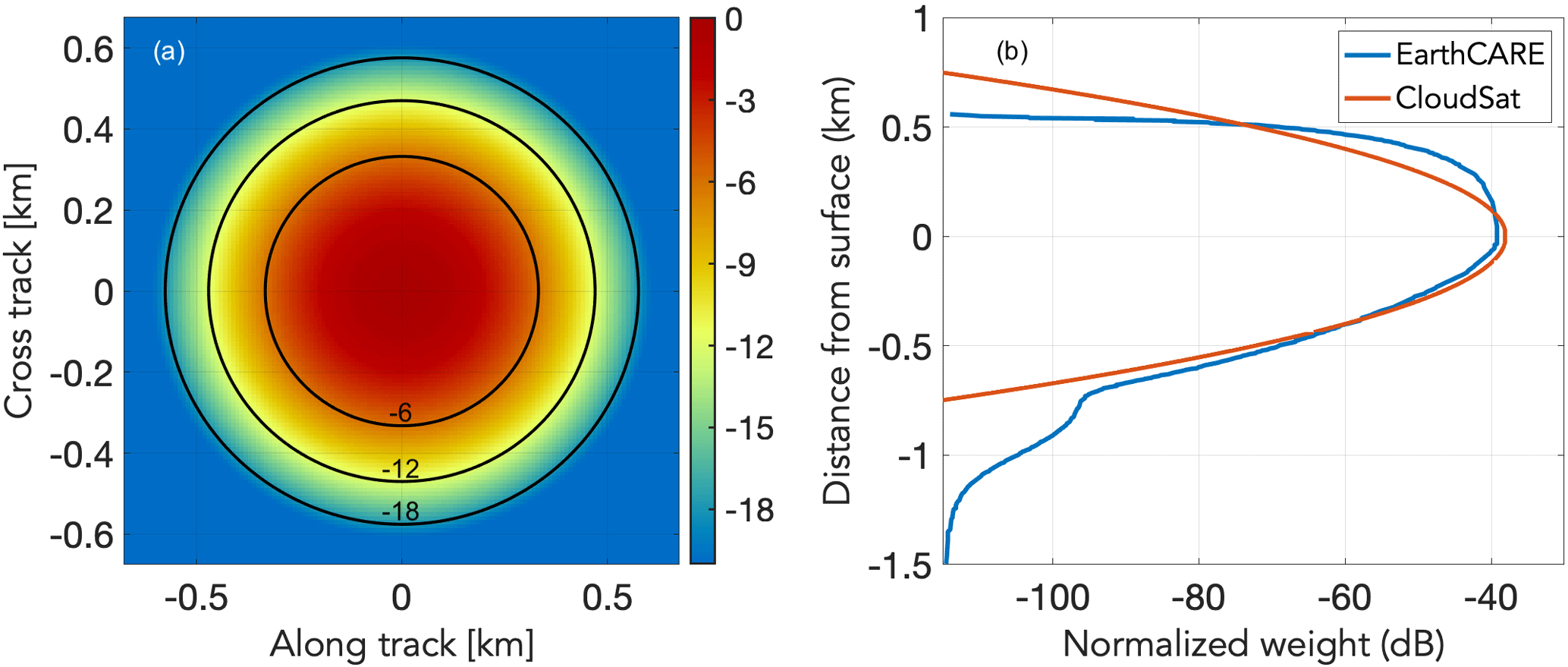
Figure 6 The EarthCARE CPR antenna weighting function W_a(x,y) distributions in the along- and cross-track direction (a). Values are in dB below the peak value. The range weighting function W_r(x,y) for CloudSat and EarthCARE (b) is also shown.

The CPR range weighting function is the result of the transmitted waveform (the same for both radar) and the CPR receiver filter. The EarthCARE CPR receiver filter was designed to sharply cut off the W_r(x,y) at 500 m above the Earth's surface to improve the detection of low-level clouds compared to CloudSat (Lamer et al., 2020). The CPR radar reflectivity at range r is estimated using the following equation:

$$\begin{array}{}\text{(27)}& Z_{\mathrm{CPR}}\left(r\right)=\sum _{i=\mathrm{1}}^{\mathrm{Gbins}}\left[Z_{\mathrm{GEM}}\left(z\right(i)-r)W_{\mathrm{r}}\left(z\right(i)-r)\right],\end{array}$$

where Gbins is the number of GEM model levels within the limits of the CPR range weighting function centered at range r. The forward simulation of the EarthCARE CPR Doppler velocity and spectrum width requires us to introduce the apparent Doppler velocity that the V_app(x) introduced to each GEM model point within the CPR footprint will have due to the satellite motion V_sat. The V_app(x) is estimated using the following equation:

$$\begin{array}{}\text{(28)}& V_{\mathrm{app}}\left(x\right)=-x{\displaystyle \frac{V_{\mathrm{sat}}}{H_{\mathrm{sat}}}},\end{array}$$

where x is the distance from nadir and H_sat is the altitude of the satellite Fig. 7. The V_app(x) is independent of the cross-track distance y; thus, $V_{\mathrm{app}}(x,y)=V_{\mathrm{app}}\left(x\right)$. At a GEM model height z, the Doppler velocity contribution V_GEM(z) to the CPR is estimated using the following equation:

$$\begin{array}{}\text{(29)}& \begin{array}{rl}{V}_{\mathrm{GEM}}\left(z\right)=& \sum _{i=\mathrm{1}}^{\mathrm{Xbins}}\sum _{j=\mathrm{1}}^{\mathrm{Ybins}}\left[Z_{\mathrm{e},m}\right(i,j\left)W_{\mathrm{a}}\right(i,j\left)\right(V_{\mathrm{app}}(i,j)\\ & +W_{\mathrm{air}}(i,j)+V_{\mathrm{SED}}(i,j)\left)\right],\end{array}\end{array}$$

where W_air(i,j) is the vertical air motion (negative is up) and V_SED(i,j) is the total sedimentation velocity at the (i,j) GEM grid point.

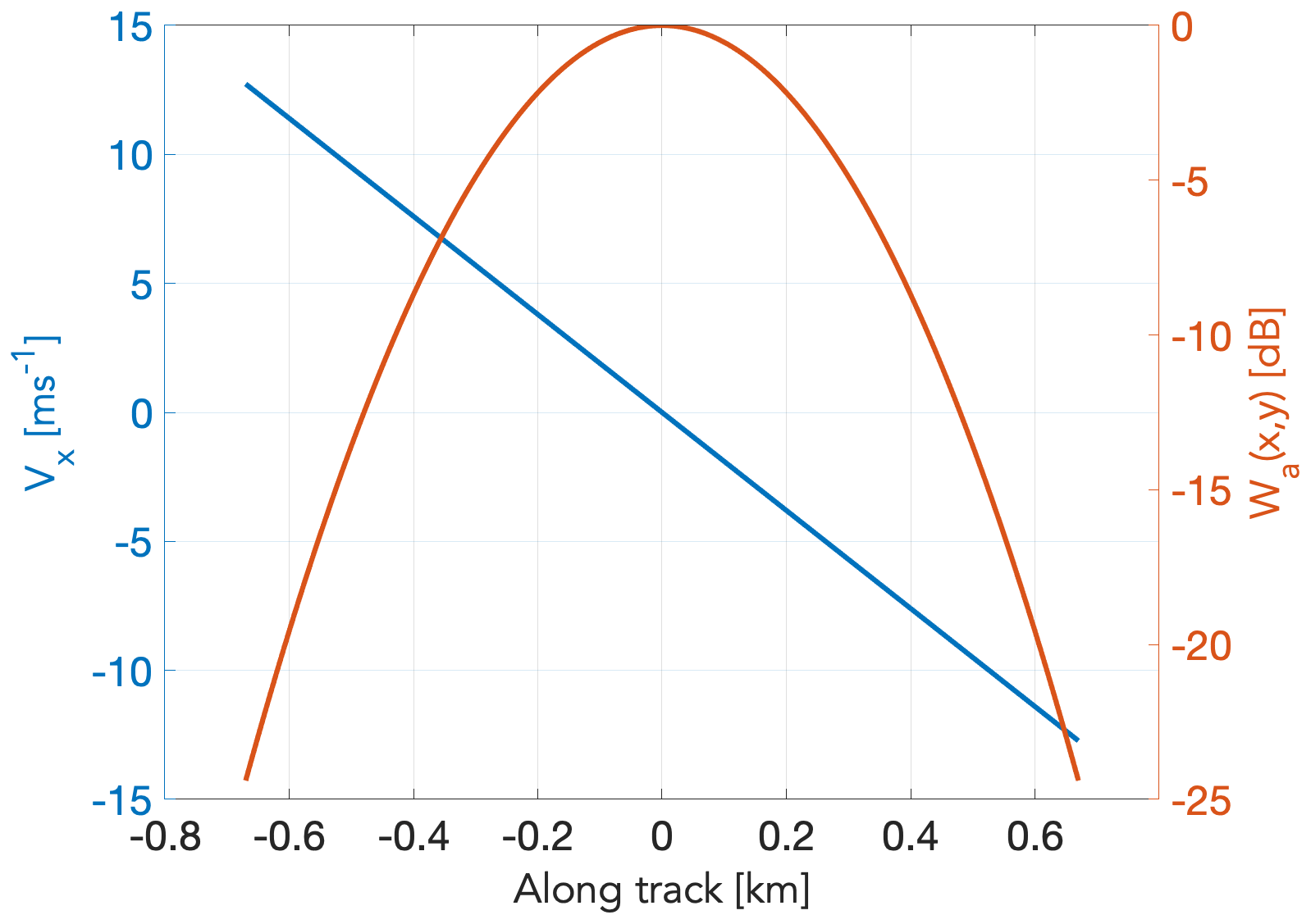
Figure 7 The EarthCARE CPR antenna weighting function W_a(x,y) and apparent Doppler velocity V_app(x) distribution as a function of distance in the along-track direction

In the CPR receiver module, the product $S_{\mathrm{v}}(i,j)=Z_{\mathrm{e},m}(i,j)W_{\mathrm{a}}(i,j)$ and the sum of all the velocity components $V_{\mathrm{tol}}(i,j)=V_{\mathrm{app}}(i,j)+W_{\mathrm{air}}(i,j)+V_{\mathrm{SED}}(i,j)$ are used to construct the periodogram S(V) mm⁶ m⁻³ m⁻¹ s) of the returned radar signal at each height z of the GEM model following the methodology proposed first by Zrnic (1975). Since we are using radar reflectivity at power, the noise is also given in radar reflectivity units (see Table 3). The periodogram is a very useful tool for describing a time series data set. In a radar system, the pulse repetition frequency (PRF) determines the temporal resolution of the time series data at a particular range gate. The periodogram is an estimate of the spectral density of a signal. The periodogram is interpolated at a spectral velocity resolution that is determined by the CPR sampling rate (PRF), which determines the higher sampled frequency. This is often called Nyquist frequency ($F_{\mathrm{N}}=\text{PRF}/\mathrm{2}$), which is half the sampling frequency of a discrete signal processing system. It is sometimes known as the folding frequency of a sampling system. Using the radar wavelength λ (Table 3), we can convert the folding frequency to folding velocity or Nyquist velocity $(V_{\mathrm{N}}=\text{PRF}\mathit{\lambda }/\mathrm{4})$. If the Doppler velocity of a radar target exceeds the magnitude of the Nyquist velocity, folding occurs (aliasing).

Once the radar receiver noise is added in the frequency domain, the next step is to perform an inverse fast Fourier transform (IFFT) of the constructed Doppler spectrum in order to retrieve I (in-phase) and Q (quadrature-phase) voltage time series (Kollias et al., 2014). The in-phase channel includes the portion of the signal in phase with the reference sinusoid. The quadrature-phase channel includes the portion of the signal 90^∘ out of phase with the reference sinusoid. The IFFT operator is applied to the amplitude spectrum. The temporal spacing of the I and Q voltages is $\mathrm{1}/\text{PRF}$. As described in Kollias et al. (2014), the I and Q time series at each GEM model height z are convoluted along range with the square root of the range weighting function W_r(x,y) and are then used as input to a pulse-pair Doppler moments estimator (Zrnic, 1977) to provide estimates of the CPR radar reflectivity, Doppler velocity, and Doppler spectrum width.

2.5 Multi-spectral imager (MSI) simulations

2.5.1 Shortwave radiative transfer calculations

The shortwave radiances for the first four EarthCARE multi-spectral imager (MSI) channels were performed by applying a one-dimensional radiative transfer model. ECSIM contains an option to perform 3D Monte Carlo calculations; however, it was unfeasible to apply this option for the totality of the domain required. The 1D calculations used DISORT with 32 streams (Lin et al., 2015) driven by the atmospheric absorption, phase functions, and surface BRDFs extracted from the scene file. The band limits and relevant atmospheric gases for the MSI SW bands are listed in Table 5 and are based on an early instrument specification, e.g., Battrick (2004). Here, for simplicity a top-hat response was assumed, and it should be noted that the exact band widths and centers differ from those of the actual instrument. The MSI retrieval algorithms make these same assumptions when applied to the simulated data; however, the detailed non-ideal spectral response of each channel will be fully accounted for when these algorithms are supplied with actual observations.

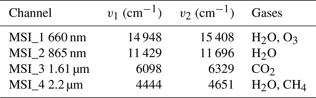
Table 5 Shortwave multispectral imager (MSI) bands; v₁ and v₂ are the effective band lower and upper wavenumber limits, respectively.

Even with a 1D approach, the computation covering the 6000×150 km frame domain at a horizontal resolution of 0.25 km is computationally demanding. In order to speed up the process, a sampling and interpolation process was implemented as follows.

• 1.

  The domain was divided into a number of sub-domains of n×m pixels. In this work these were n=12 and m=12.

• 2.

  For each pixel in the sub-domain, the quantities $X_{\mathrm{1}}(i,j)=A_{\mathrm{s}}(i,j)\exp (-\mathit{\tau }(i,j\left)\right)$ and $X_{\mathrm{2}}(i,j)=\exp (-\mathit{\tau }(i,j\left)\right)$ were calculated, where τ is the particulate optical depth and A_s is the pixel black-sky albedo.

• 3.

  Within each subdomain, the pixels where DISORT would be applied to were selected using the following method:

  • a.

    the lower left pixels were selected by default;

  • b.

    in the along-track direction, each ith and jth pixel are selected by default (in this work, every fifth pixel was used);

  • c.

    the pixels along the spacecraft nadir track are selected by default;

  • d.

    the pixels with the maximum and minimum values of X₁ and X₂, respectively, are selected.

• 4.

  For each of the selected pixels, DISORT was used to calculate the top-of-atmosphere (TOA) radiances.

• 5.

  For each of the non-selected pixels (denoted by i_n, j_n) the radiance of the selected pixels (i_s, j_s) is scanned through, and the pixel that minimizes $\text{abs}\left(X_{\mathrm{1}}(i_{\mathrm{n}},j_{\mathrm{n}})-\left(X_{\mathrm{1}}(i_{\mathrm{s}},j_{\mathrm{s}})\right)\right)+\text{abs}\left(X_{\mathrm{2}}(i_{\mathrm{n}},j_{\mathrm{n}})-\left(X_{\mathrm{2}}(i_{\mathrm{s}},j_{\mathrm{s}})\right)\right)$ is used to fill in the TOA radiance.

• 6.

  The domain was shifted by half its width in the along-track direction and then shifted in the cross-track direction when the end of the frame was reached, with the process repeated until the entire frame was covered. The overlap between domains was found to be useful for eliminating artifacts mimicking the sub-domain structure.

The procedure was able to speed-up the necessary calculation by an order of magnitude while retaining a suitable degree of accuracy. For example, for the “Halifax scene” (see Sect. 3), when smoothed to the MSI resolution of 1 km × 1 km and referring to the MSI CH1 BRDF, 65 % of the resulting errors were less than 0.1 %, 87 % of the errors were within 1 %, and 99 % of the errors were less than about 5 %. As may be expected, the larger errors are associated with sharp cloud edges. The low error is mainly due to the high degree of correlation in the clouds fields for distances less than 1.5 km or so. This echoes the findings of Barker and Li (2019).

Of course, by neglecting 3D radiative transfer effects the simulations are not as realistic as they might be. It is well known that 3D effects can have especially large effects on the measured radiances, e.g., Barker and Liu (1995). However, it should be noted that apart from drastically reducing the computational requirements, there is one additional technical benefit in performing the simulations using 1D radiative transfer. That is the fact that the MSI retrieval algorithms (e.g., Hünerbein et al., 2023), while still being state-of-the-art methods, are based on 1D radiative transfer theory. Thus, the 1D simulations are better suited for the technical evaluation of these algorithms even though the 3D simulations are less realistic. It should also be noted that the use of the scenes for 3D RT studies is ongoing and that 3D effects are being addressed in the EarthCARE radiative closure evaluation (Cole et al., 2023).

After the MSI shortwave calculations were performed (at a resolution of 0.25 km), the radiances were binned to the MSI instrument resolution (1 km), and the effects of instrument random noise were simulated using a Gaussian pseudo-random number generator. Technical details of the MSI can be found in Chang (2019).

2.5.2 Longwave radiative transfer calculations

Like the shortwave MSI calculations, the TOA radiances for the longwave MSI channels (see Table 6) were calculated using DISORT. Since the longwave calculations are not as computationally demanding as the shortwave calculations, no sampling strategy was necessary, and DISORT with 16 streams specified was applied to every pixel in the MSI frame domain.

Table 6 Longwave multispectral imager (MSI) bands.

As was the case with the shortwave channels, the idealized radiances at 0.25 km resolution were binned to the MSI instrument resolution (1 km), and the effects of instrument random noise were simulated using a Gaussian pseudo-random number generator.

2.6 Broadband radiometer (BBR) simulations

The methods described for the MSI short and longwave TOA radiances were applied to the BBR calculations for the spectral-band resolved BBR TOA radiances for each of the three BBR views as well as the TOA fluxes. The shortwave bands used are listed in Table 7, and longwave bands are listed in Table 8.

Table 7 Center wavelengths used for broadband shortwave calculations and relevant gases.

Table 8 Center wavelengths used for broadband longwave calculations and relevant gases.

The BBR ideal radiances at 250 m resolution as calculated by the radiative transfer code were used to create simulated L1-b data, i.e., BBR filtered radiances (B-NOM) and BBR single-pixel filtered radiances (B-SNG); see the production model in Eisinger et al., 2023). This process first involved the convolution of the simulated radiances with the spectral responses of the BBR instrument to obtain broadband SW, L_SW, and LW, L_LW, radiances at 250 m. Secondly, as the BBR instrument will measure total-wave (TW) radiances, which are not simulated, the TW (L_TW) radiances at 250 m resolutions are calculated as the weighted sum of the longwave and shortwave channels (i.e., $L_{\mathrm{TW}}=L_{\mathrm{LW}}+A\cdot L_{\mathrm{SW}}$) (Velázquez Blázquez et al., 2023).

In order to simulate realistic L1 B-SNG inputs, the chopper drum mechanism (CDM) speed has to be taken into account. It has been configured at a 0.7 ratio of the original nominal speed, as recommended to maximize the lifetime of the mechanism, which defines a ground sampling distance for two consecutive SW or TW measurements of 1.1 km. The current BBR simulator software to produce the B-SNG input performs a bilinear interpolation of the 250 m broadband radiances at the positions of the 30-detector array, and this is done for each of the BBR views (fore, nadir and aft). The resulting B-SNG SW and TW radiances for the Halifax scene (Sect. 3.1) are show in Figs. 8 and 9. Finally, a domain integration or point spread function weighting is done to pass from the single-pixel radiances in B-SNG to the nominal BBR resolutions in B-NOM (standard, full and small) sampled every 1 km.

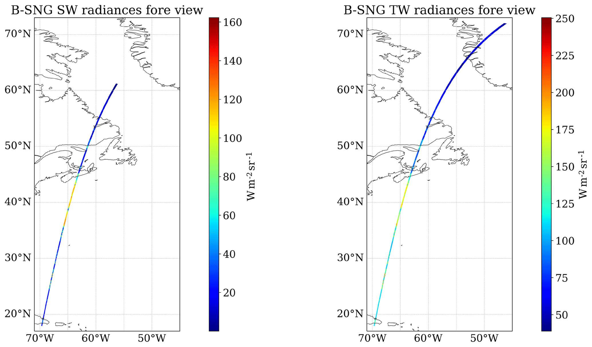
Figure 8 Simulated B-SNG TOA broadband radiances for the fore view of the BBR SW and TW channels for the Halifax scene. Similar plots are obtained for the nadir and aft views.

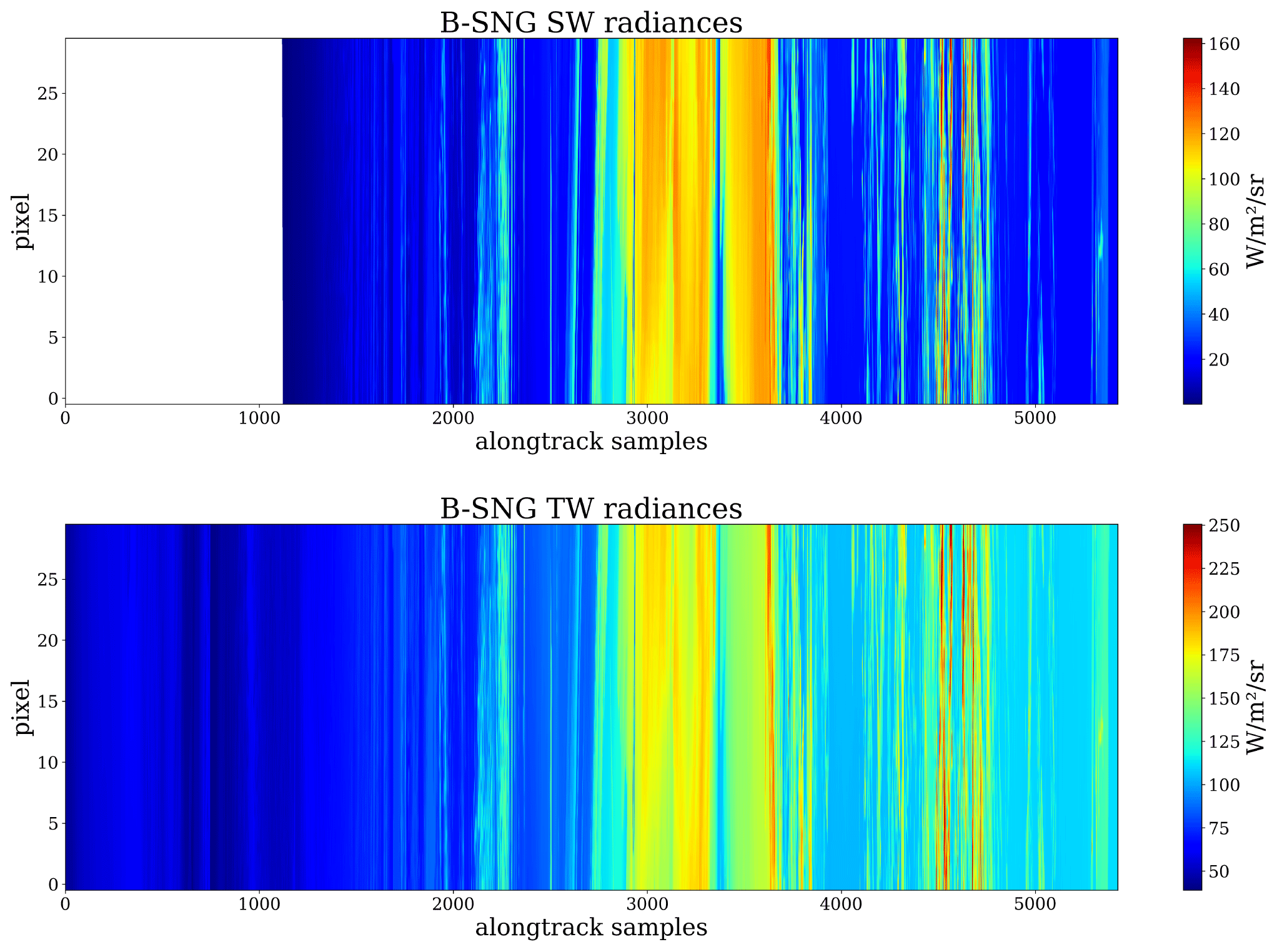
Figure 9 Simulated B-SNG TOA broadband radiances for the fore view of the BBR SW and TW channels for the Halifax scene.​​​​​​​

3 The test frames

In this section, simulated L1 data for the EarthCARE test scenes are presented and discussed. The level 1 simulated data and various model truth fields for three GEM-derived scenes are available from https://doi.org/10.5281/zenodo.7117115 (van Zadelhoff et al., 2023a).

3.1 Halifax

The high-latitude part of the Halifax scene features mixed-phase clouds at nighttime, transitioning from deeper clouds with tops up to 6 km around 65^∘ N featuring supercooled liquid in convective cells, to mixed-phase clouds with tops around 3 km at temperatures as cold as −30 ^∘C, and finally to more broken shallow mixed-phase clouds toward 50^∘ N. Near the center of the frame, a storm system with supercooled layers, convective precipitation, and ice clouds with tops up to altitudes of 13 km is present. South of about 45^∘ N, cloud-free and shallow low-altitude water clouds are present. Also south of 45^∘ N, extended aerosol regions are present. From the ground to above 2 km a marine layer (mainly sea salt) is present and above this a thinner continental pollution layer (mainly fin-mode non-absorbing aerosol) is present. The differences in the lidar ratio associated with these two aerosol regions shown in the middle panel of Fig. 10 is evident.

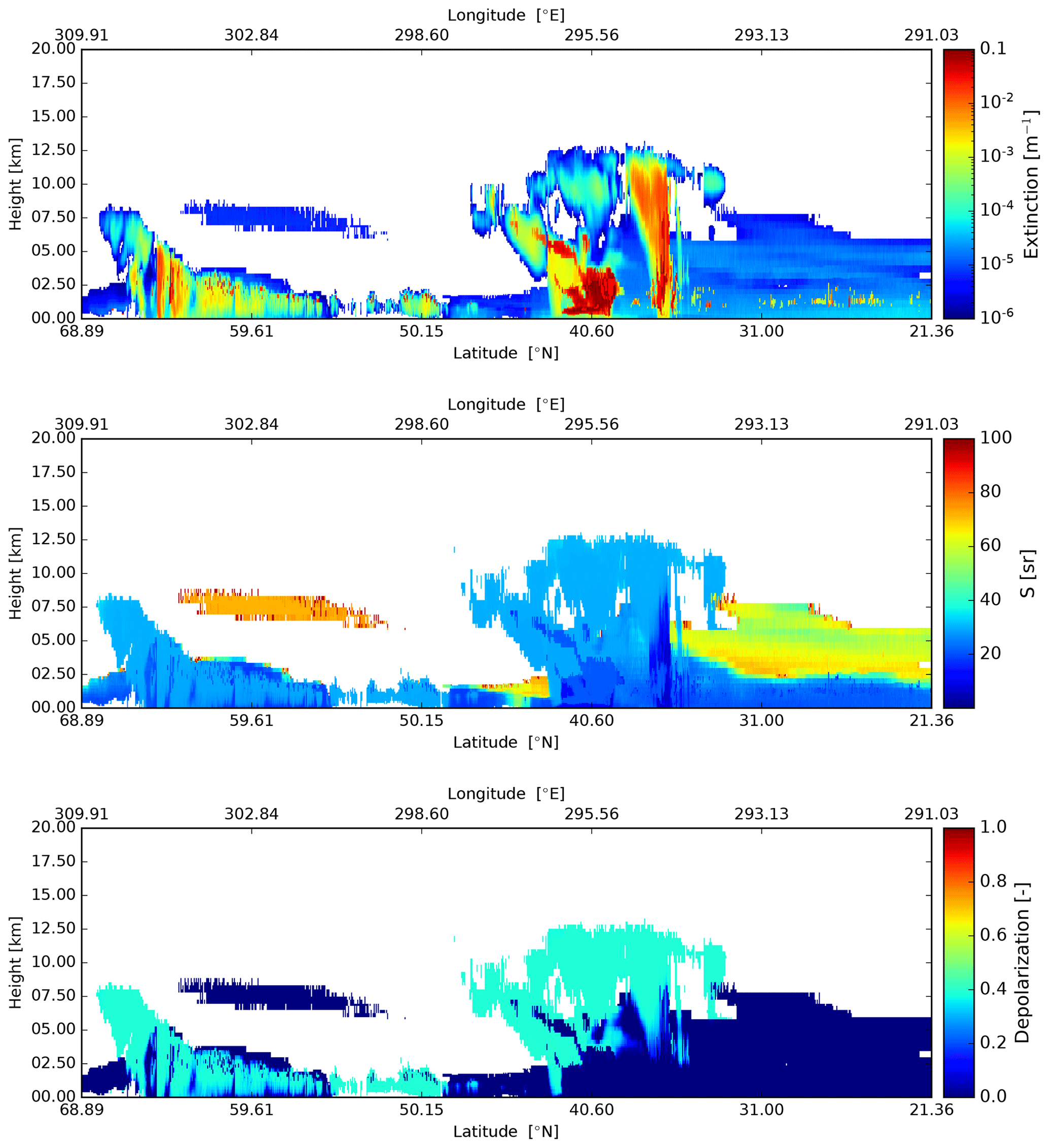
Figure 10 Cross-sections of the extinction at 355 nm, lidar extinction-to-backscatter ratio, and linear depolarization ratio, following the simulated EarthCARE orbit for the Halifax scene.

The simulated ATLID Mie, Rayleigh, and cross-polar attenuated backscatters are shown in Fig. 11. It can be seen that the lidar penetration into the clouds is limited, as expected, especially in the central part of the frame. However, most of the ice clouds are captured well. The aerosol fields in the southern segment of the frame are also well captured. Quantitative measures of the ability to detect features in the ATLID data are presented in van Zadelhoff et al. (2023b), which describes the ATLID feature mask product (A-FM). The accuracy and sensitivity of quantitative cloud and aerosol extinction and backscatter retrievals applied to the ATLID data are discussed in, e.g., Donovan et al. (2023) and Mason et al. (2023).

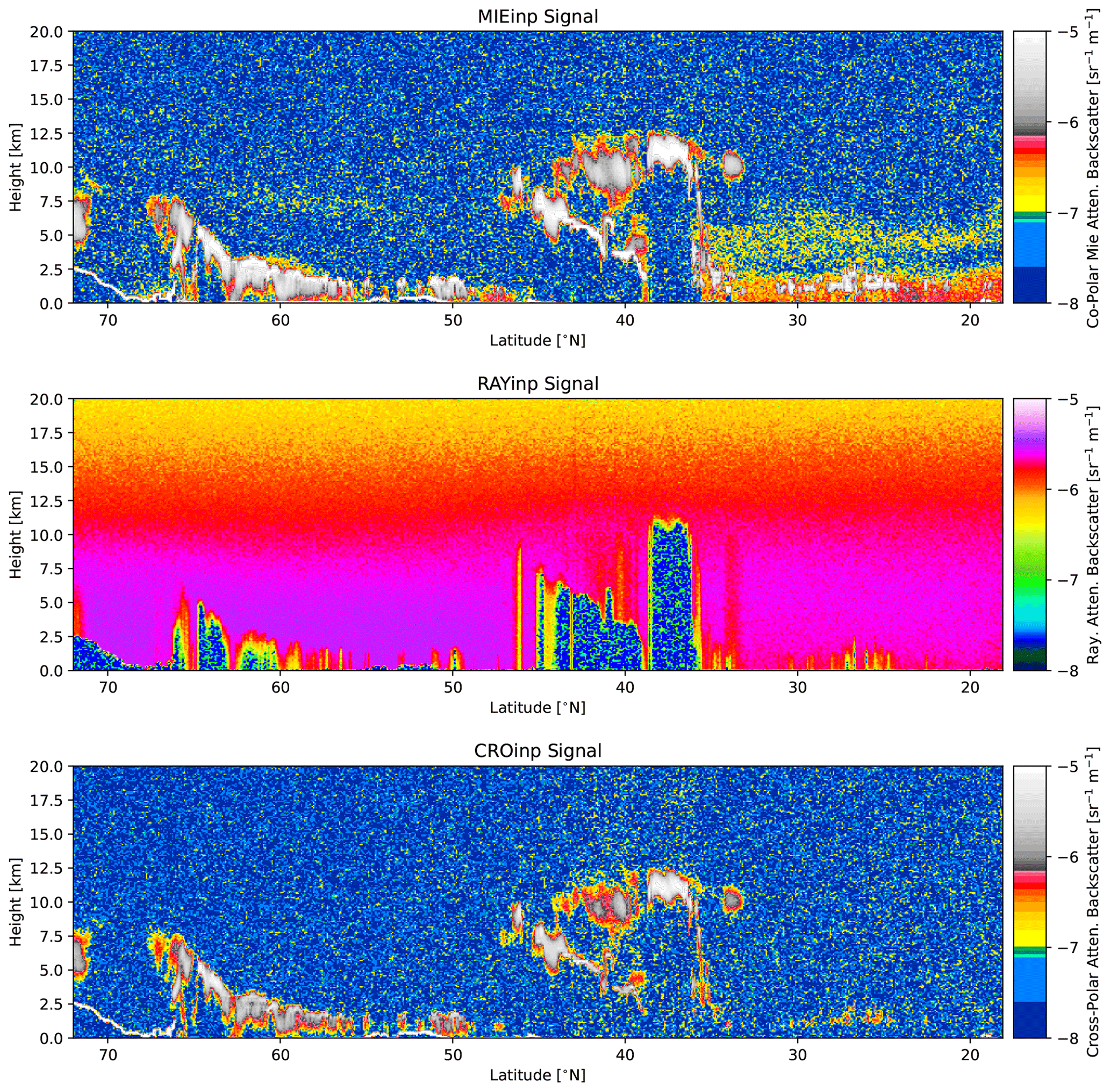
Figure 11 Simulated Mie channel, Rayleigh channel, and cross-polar ATLID attenuated backscatters for the Halifax scene.

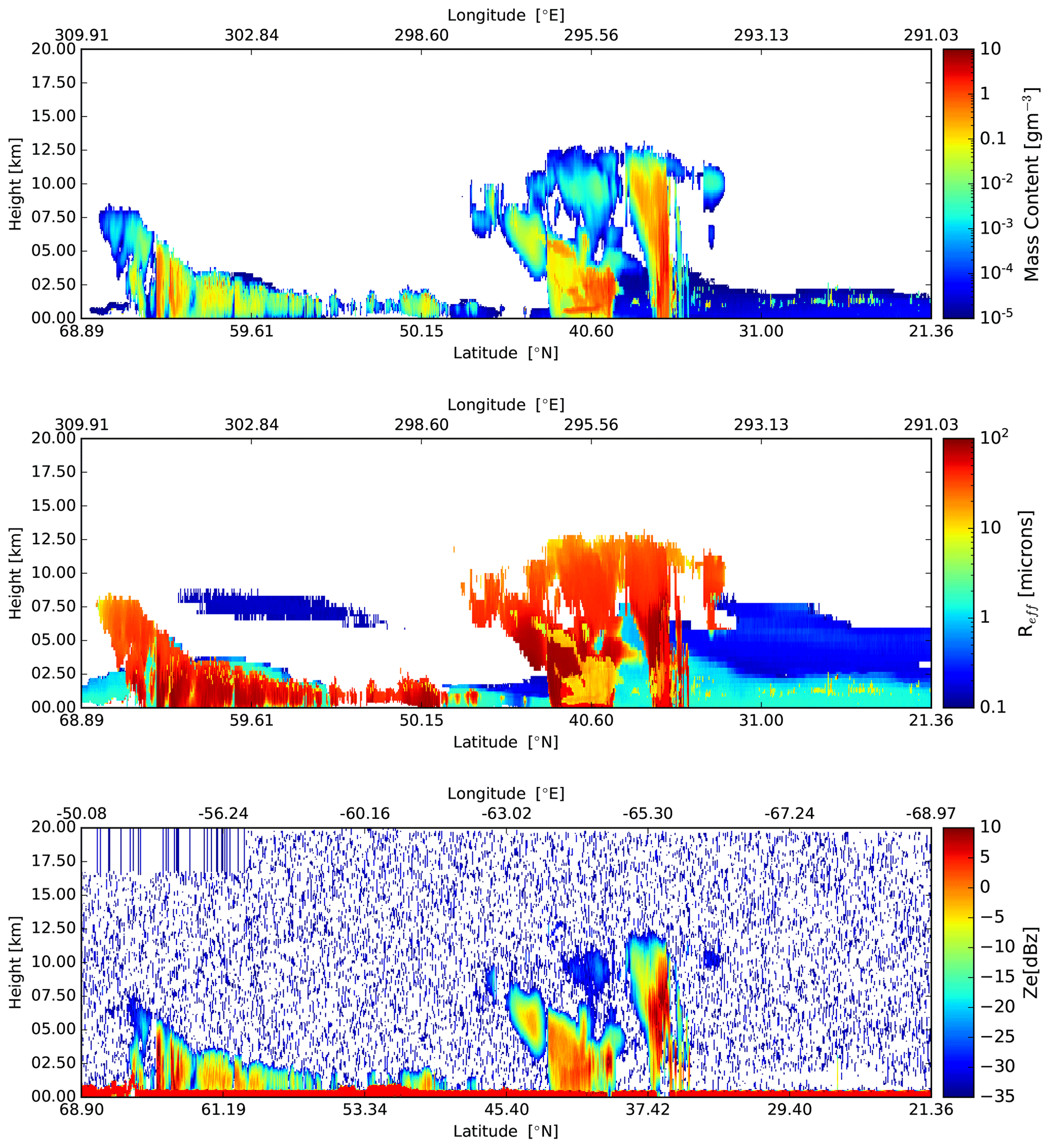
Figure 12 Cross-sections of the particle mass density, effective particle radius, and simulated observe radar reflectivity, following the simulated EarthCARE orbit for the Halifax scene.

The nadir fields of particle mass, effective radius, and simulated observed radar reflectivity for the full Halifax scene are shown in Fig. 12. The striped area in the radar reflectivity present in the upper-left of the lower panel is due to a simulated change in maximum height covered by the radar, which is associated with a latitude-dependent change in the operating PRF. Radar reflectivity is a strong function of the particle effective radius; hence, in general the larger effective radii regions of the scene are well sampled, while areas containing relativity small water cloud droplets are not.

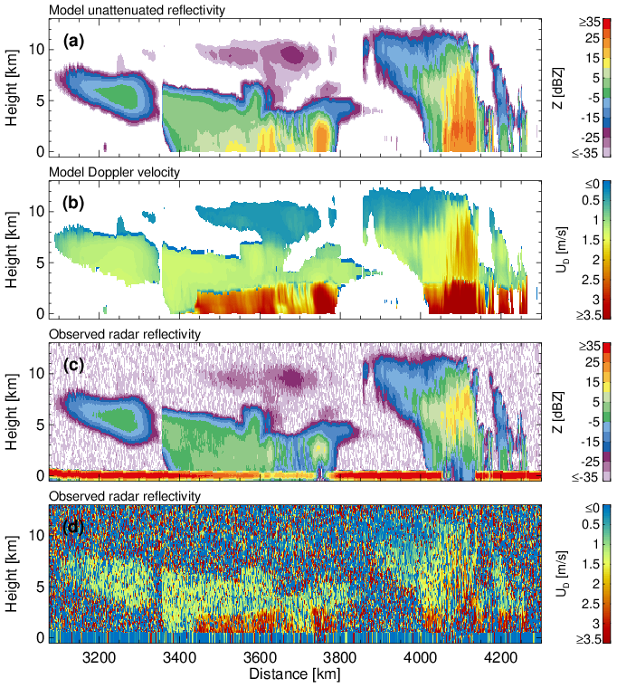
Figure 13 (a) GEM unattenuated 94 GHz radar reflectivity factor at the model resolution, (b) GEM sedimentation Doppler velocity at the model resolution, (c) CPR raw radar reflectivity factor at the CPR resolution with surface echo, and (d) CPR raw Doppler velocity measurements with no correction applied at the CPR resolution with surface echo.

The GEM model and CPR-simulated signals for a selected region of the Halifax scene are shown in Fig. 13. Due to the large horizontal extent of the scene, we focus on the 30–48^∘ N simulated region that covers the frontal and convective systems. The top two panels shows the unattenuated 94 GHz radar reflectivity and the reflectivity-weighted hydrometeor sedimentation velocity at the GEM grid resolution. The two systems are characterized by high cloud tops (12 km), periods with thick high-level clouds, and extensive periods with light and moderate precipitation. The lower two panels show the raw (uncorrected) CPR radar reflectivity and mean Doppler velocity measurements. The EarthCARE CPR has sufficient sensitivity to detect the hydrometeor layers except weak reflectivity echoes near the highest cloud tops. The strong 94 GHz attenuation by hydrometeors results in missed detections near the surface. This can be clearly seen by the depression of the surface echo radar reflectivity at 3700 km and the complete loss of the surface echo around 4100 km. The faint CPR echoes that fill the surface echo gap around 4100 km are due to multiple scattering (Battaglia et al., 2010). As expected, the CPR raw Doppler velocity field (500 m along-track integration) is noisy (Kollias et al., 2014, 2022). The post-processing algorithm described in Kollias et al. (2023) is expected to significantly improve the quality of the CPR Doppler velocity measurements. Despite their noisiness, the CPR Doppler velocities reproduce the main features of the GEM model Doppler velocities, namely the transition from solid to liquid hydrometeors and the low-sedimentation Doppler velocities in the upper cloud levels. More details concerning the performance of the CPR and the CPR cloud algorithms are provided in Mroz et al. (2023) and Kollias et al. (2002).

The simulated shortwave TOA radiances for the MSI shortwave channels are shown in Fig. 14. Here, north of about 55^∘ N the Sun is below the horizon so that the radiances are zero. Below about 42^∘ N, the swath is above the ocean with the exception of passing over the Dominican Republic near the southern frame border. The NDVI (normalized difference vegetation index, defined as the difference in reflectances divided by their sum for the two indicated channels) fields corresponding to the radiances shown in Fig. 14 are shown in Fig. 15.

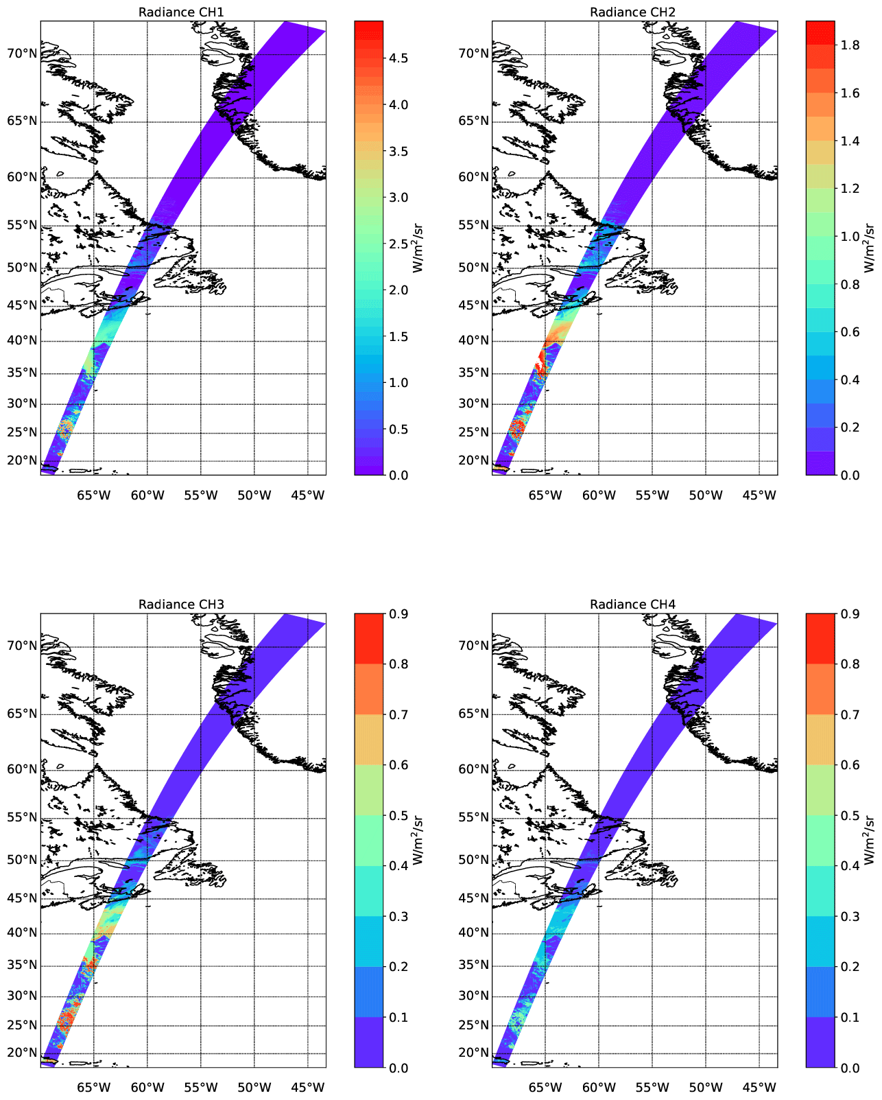
Figure 14 Simulated TOA radiances for the four SW EarthCARE MSI channels for the Halifax scene.

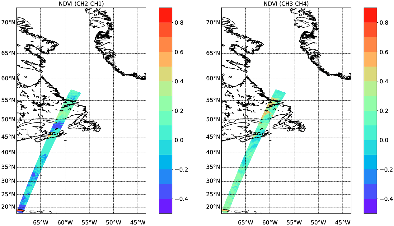
Figure 15 NDVI values corresponding to the simulated radiances shown in Fig. 14.

The simulated longwave TOA brightness temperatures for the MSI longwave channels are shown in Fig. 16. Here cold (but low-altitude) clouds tops north of 55^∘ N are visible, as are the cold (but high) cloud top temperatures between 35 and 45^∘ N. The warm land and ocean temperatures are also apparent in the mainly cloud-free region south of about 35^∘ N. A close-up of the channel 1 radiances for the Halifax scene between 32.5 and 37.5^∘ N can be seen within Fig. 17.

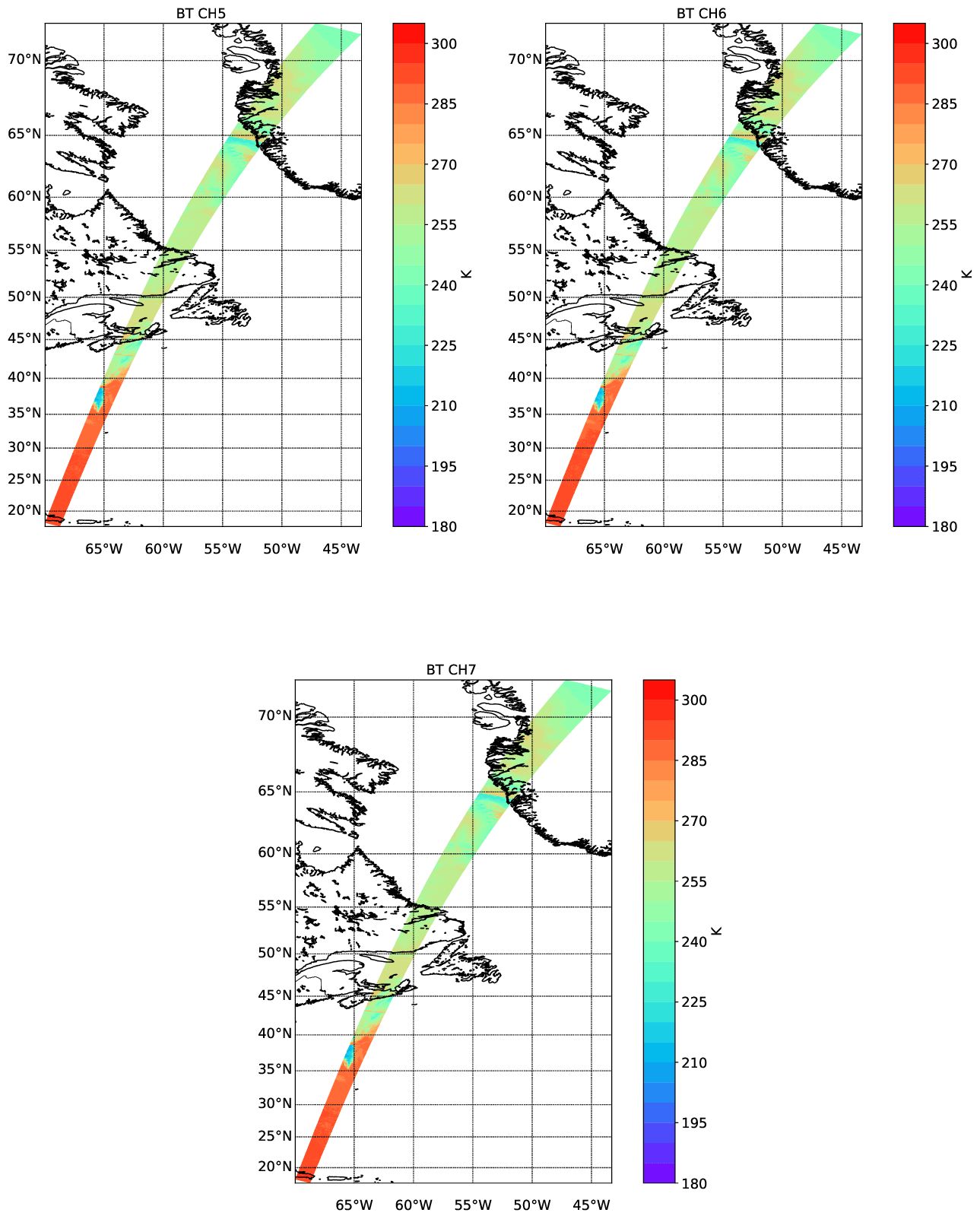
Figure 16 Simulated TOA brightness temperatures for the three LW EarthCARE MSI channels for the Halifax scene.

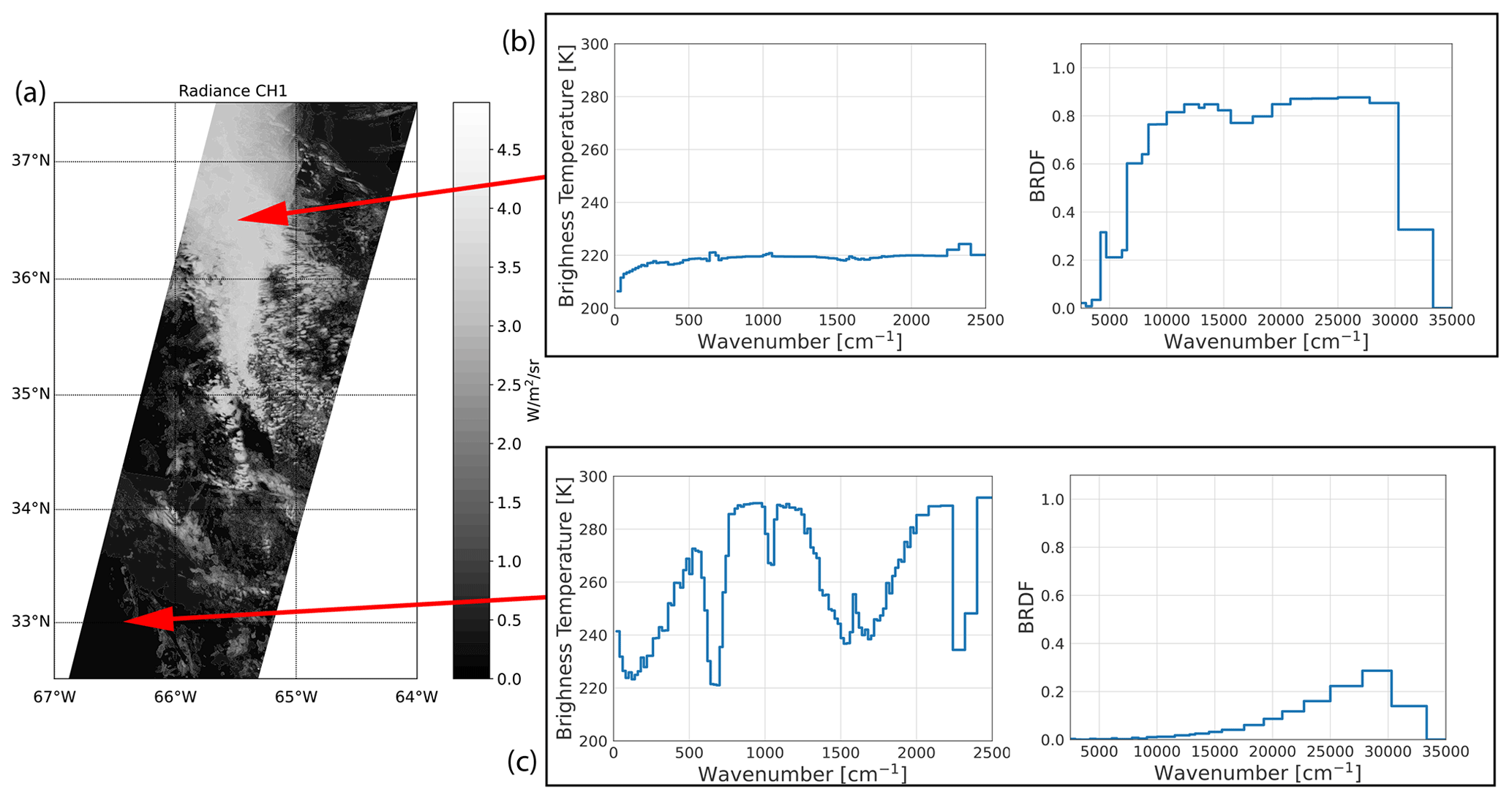
Figure 17 (a) TOA channel 1 radiances for the Halifax scene between 32.5 and 37.5^∘ N. (b) LW brightness temperatures and SW BRDFs as a function of wavenumber corresponding to a high-altitude thick cloud. (c) LW brightness temperatures and SW BRDFs for each BBR channel corresponding to cloud-free conditions over ocean.

3.2 Baja

The Baja scene is the second GEM-derived scene. This scene has a lot of topographical variation compared to the Halifax scene and contains large regions of thinly distributed aerosols. In addition, high-level ice clouds are present south of 35^∘ N. Near the center of the scene, above the Rocky Mountains, extended regions of optically thick ice and water clouds are present.

The extinction, lidar radio, and depolarization model truth fields for the nadir track are shown in Fig. 18. The lidar-observed attenuated backscatter fields are shown in Fig. 19, while the particle mass density, effective radius, and equivalent radar reflectivity are shown in Fig. 20.

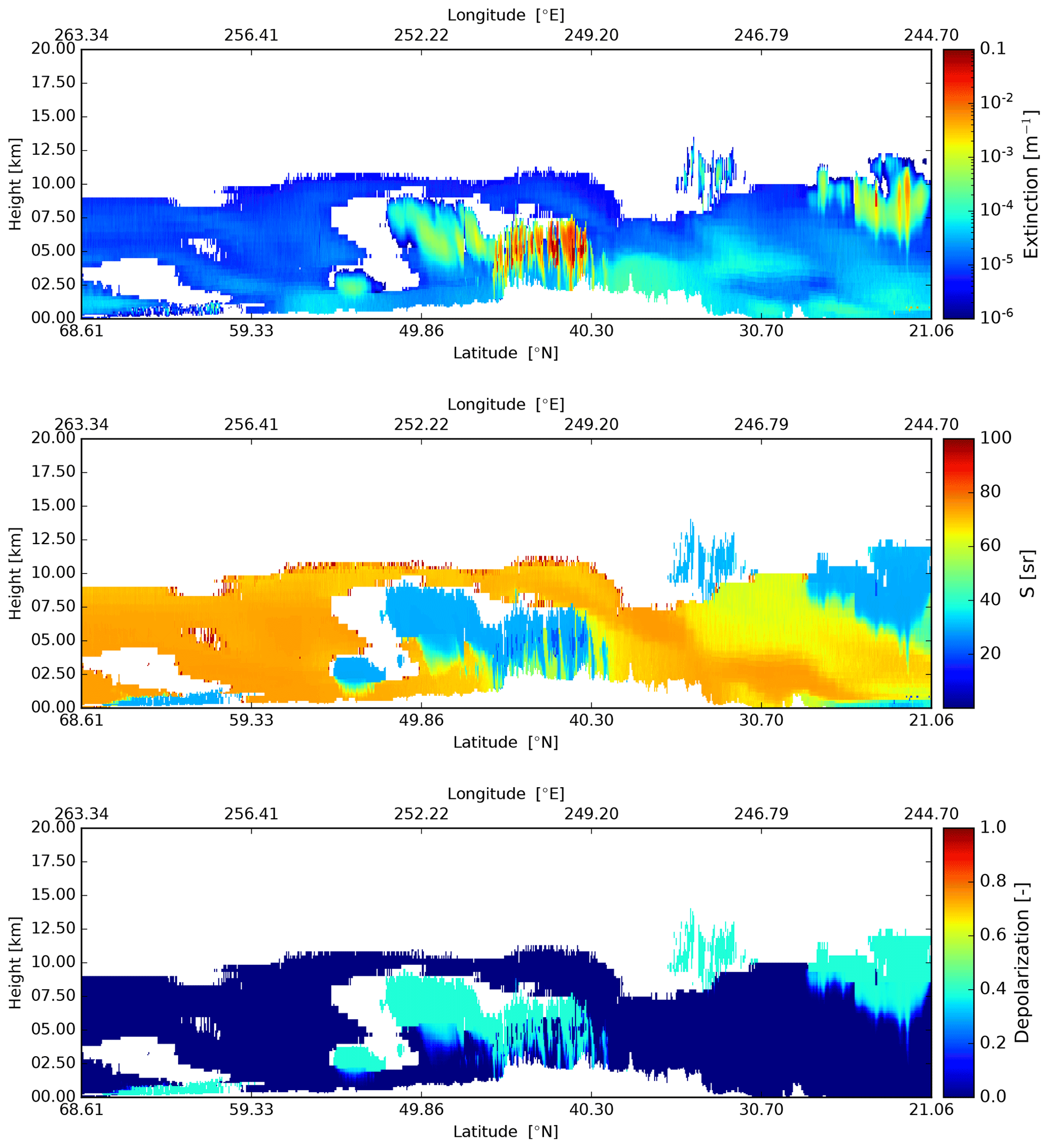
Figure 18 Cross-sections of the extinction at 355 nm, lidar extinction-to-backscatter ratio, and linear depolarization ratio, following the simulated EarthCARE orbit for the Baja scene.

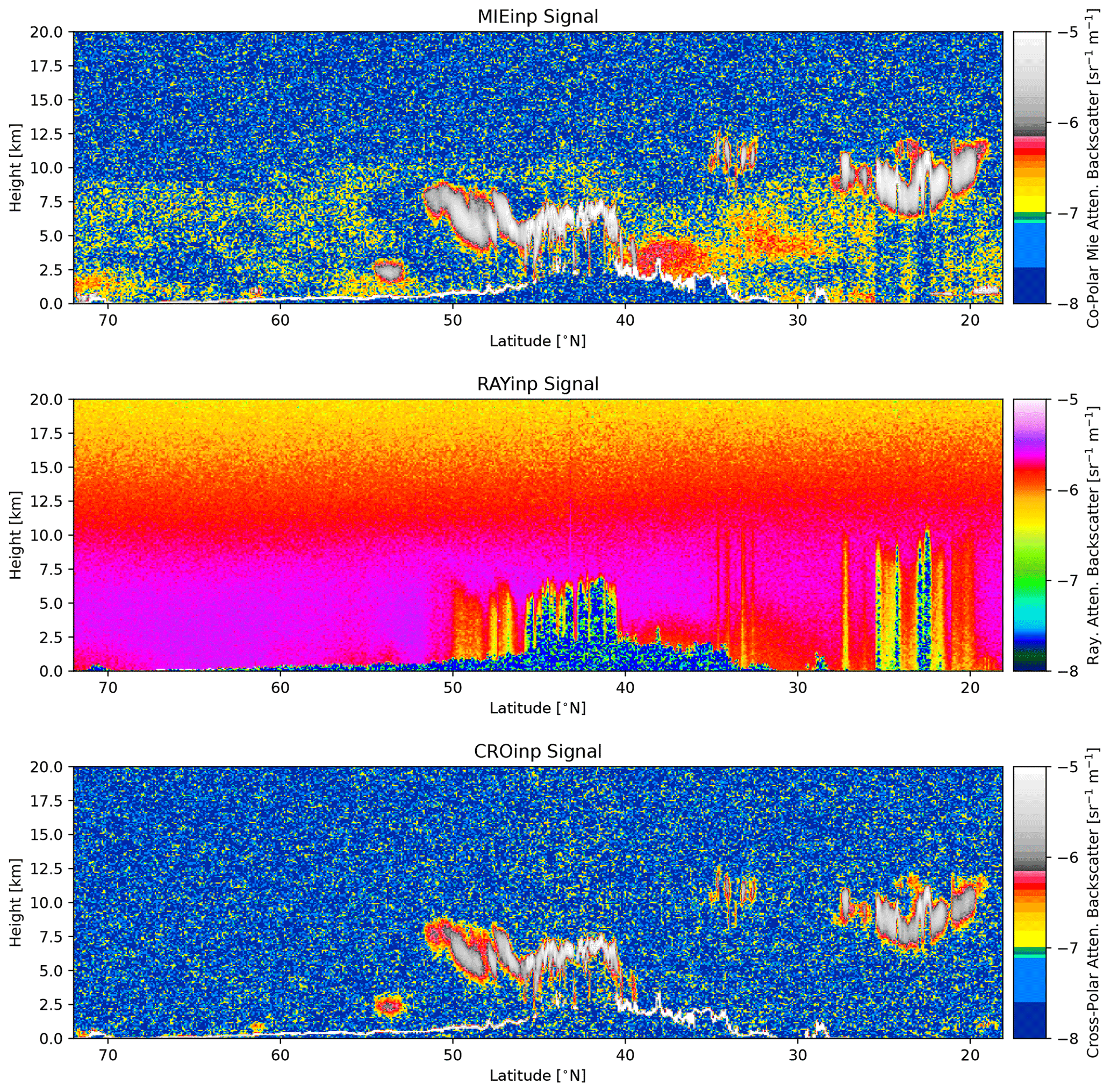
Figure 19 Simulated Mie channel, Rayleigh channel, and cross-polar ATLID attenuated backscatters for the Baja scene.

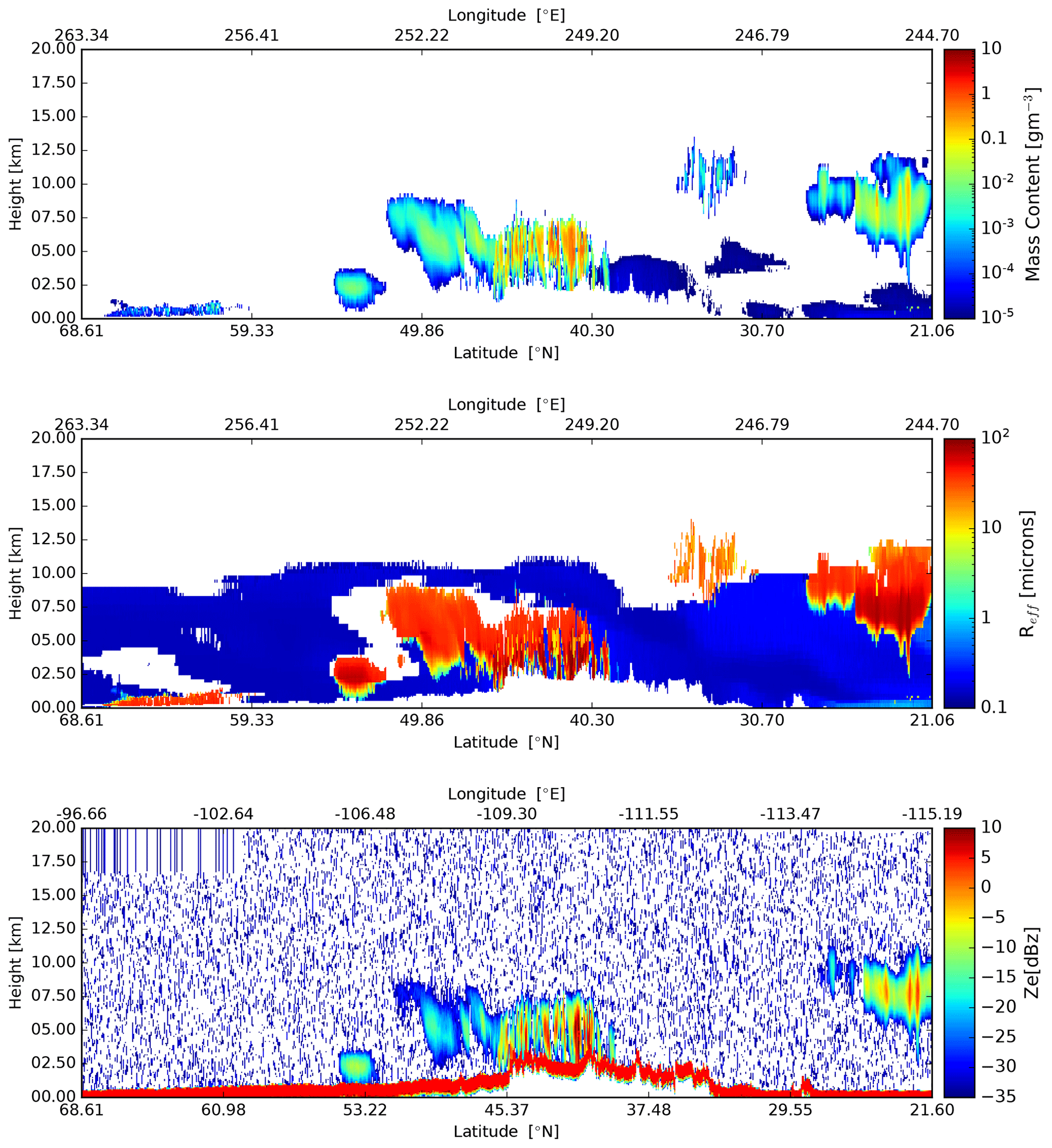
Figure 20 Cross-sections of the particle mass density, effective particle radius, and observed radar reflectivity, following the simulated EarthCARE orbit for the Baja scene.

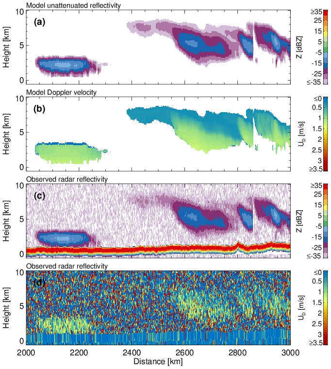
Figure 21 (a) GEM unattenuated 94 GHz radar reflectivity factor at the model resolution, (b) GEM sedimentation Doppler velocity at the model resolution, (c) CPR raw radar reflectivity factor at the CPR resolution with surface echo, and (d) CPR raw Doppler velocity measurements with no correction applied at the CPR resolution with surface echo.

The GEM model and CPR-simulated signals for a selected region of the Baja scene are shown in Fig. 21. Due to the large horizontal extent of the scene, we focus on the 45–55^∘ N simulated region that covers the northern part of the GEM simulation over the Rockies that includes ice clouds. The top two panels shows the unattenuated 94 GHz radar reflectivity and the reflectivity-weighted hydrometeor sedimentation velocity at the GEM grid resolution. The ice clouds are characterized by low radar reflectivity and Doppler velocities that increase towards the hydrometeor layer base. Due to their low radar reflectivity, a significant fraction of the EarthCARE CPR echoes are close to its detection limit (−35 dBZ). The low radar reflectivities contribute to the noisiness of the CPR raw Doppler velocities.

The simulated shortwave TOA radiances for the MSI shortwave channels are shown in Fig. 22. Here, north of about 55^∘ N snow and ice surfaces are present, leading to high channel 1 and 2 radiances even when clear-sky conditions are present. The snow and ice surfaces also stand out in the CH3-CH4 NDVI images (Fig. 23).

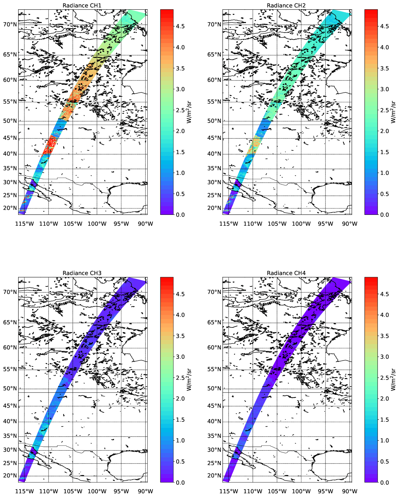
Figure 22 Simulated TOA radiances for the four SW EarthCARE MSI channels for the Baja scene.

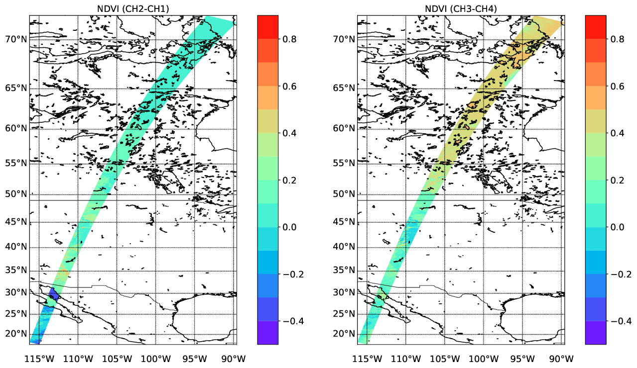
Figure 23 NDVI values corresponding to the simulated radiances shown in Fig. 22.

The simulated longwave TOA brightness temperatures for the MSI longwave channels are shown in Fig. 24. Here there are cold (but low-altitude) cloud tops and surfaces north of 55^∘ N visible, as well as cold (but high) cloud top temperatures around 45^∘ N. The warm land and ocean temperatures are also apparent in the mainly cloud-free region south of about 40^∘ N.

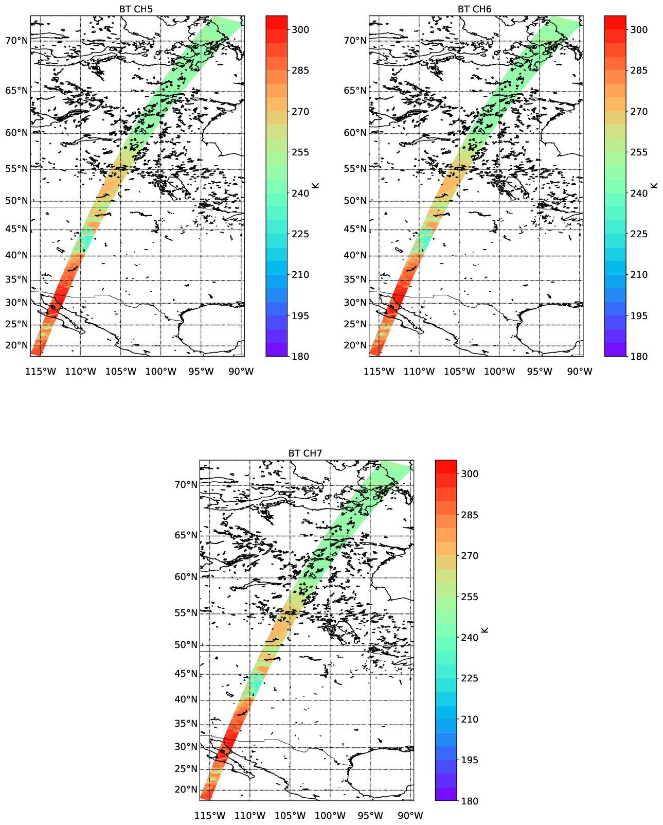
Figure 24 Simulated TOA brightness temperatures for the three LW EarthCARE MSI channels for the Baja scene.

3.3 Hawaii

The third GEM-based scene is the Hawaii scene, situated almost completely over ocean, where the nadir track is completely over ocean and a few of the smaller Hawaiian islands are within the MSI track. This scene exhibits areas of clear sky, upper-level cirrus, and a tropical convective system near the center of the scene. The extinction, lidar ratio, and depolarization model truth fields for the nadir track are shown in Fig. 25. The lidar-observed attenuated backscatter fields are shown in Fig. 26, while the particle mass density, effective radius, and equivalent radar reflectivity are shown in Fig. 27.

Figure 25 Cross-sections of the extinction at 355 nm, lidar extinction-to-backscatter ratio, and linear depolarization ratio, following the simulated EarthCARE orbit for the Hawaii scene.

Figure 26 Simulated Mie channel, Rayleigh channel, and cross-polar ATLID attenuated backscatters for the Hawaii scene.

Figure 27 Cross-sections of the particle mass density, and effective particle radius, and observed Radar reflectivity, following the simulated EarthCARE orbit for the Hawaii scene.

Figure 28 (a) GEM unattenuated 94 GHz radar reflectivity factor at the model resolution, (b) GEM sedimentation Doppler velocity at the model resolution, (c) CPR raw radar reflectivity factor at the CPR resolution with surface echo, and (d) CPR raw Doppler velocity measurements with no correction applied at the CPR resolution with surface echo.

The GEM model and CPR-simulated signals for the Hawaii scene are shown in Fig. 28. Due to the large horizontal extent of the scene, we focus on the center of the scene where a large tropical convective and stratiform precipitating system was simulated. The top two panels show the unattenuated 94 GHz radar reflectivity and the reflectivity-weighted hydrometeor sedimentation velocity at the GEM grid resolution. The widespread stratiform precipitation is extensive, covering over 500 km, and the precipitation system reaches tops of 16 km. Embedded convective cells are simulated at 2375 and 2750 km along-track distance. The lower two panels show the raw (uncorrected) CPR radar reflectivity and mean Doppler velocity measurements. The EarthCARE CPR has sufficient sensitivity to detect the hydrometeor layers, except for weak reflectivity echoes near the highest cloud tops. The strong 94 GHz attenuation by hydrometeors results in significant attenuation in the rain layer and complete loss of the surface echo return in the two embedded convective cells. Significant multiple scattering is simulated at 2750 km, as seen by the faint CPR echoes that fill the surface echo gap around 4100 km (Battaglia et al., 2010). As expected, the CPR raw Doppler velocity field (500 m along track integration) is noisy (Kollias et al., 2014, 2022). Despite their noisiness, the CPR Doppler velocities reproduce the main features of the GEM model Doppler velocities, namely, the transition from solid to liquid hydrometeors and the low-sedimentation Doppler velocities in the upper cloud levels.

The simulated shortwave TOA radiances for the MSI shortwave channels are shown in Fig. 29. Here the cloud features are all clearly visible against the low-albedo ocean. The NDVI fields are shown in Fig. 30. The high values in the right panel correspond to one of the few land areas (the island of Niihau) within the MSI swath.

Figure 29 Simulated TOA radiances for the four SW EarthCARE MSI channels for the Hawaii scene.

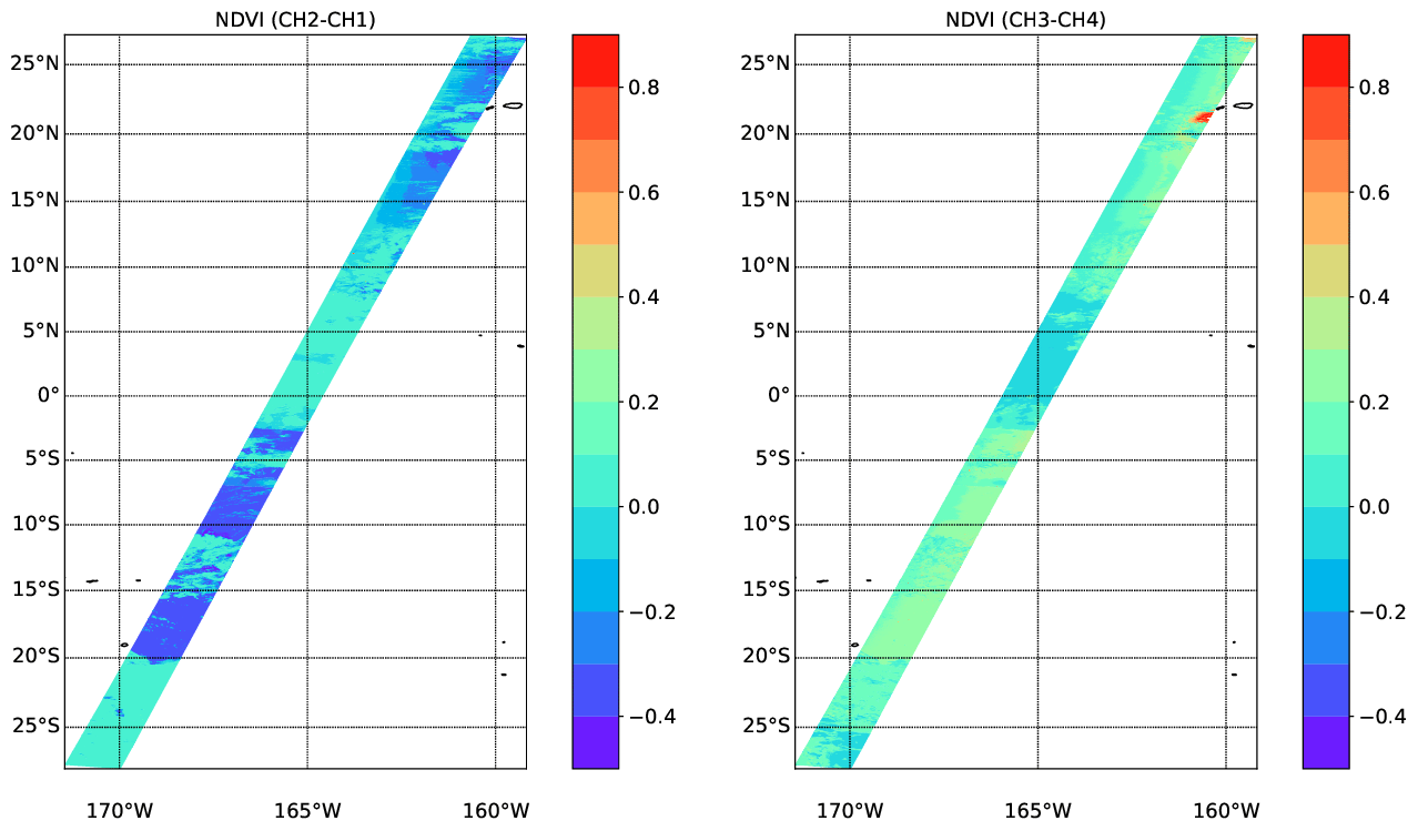
Figure 30 NDVI values corresponding to the simulated radiances shown in Fig. 29.

The simulated longwave TOA brightness temperatures for the MSI longwave channels are shown in Fig. 31. Here the very cold cloud tops near the center of the scene are especially prominent.

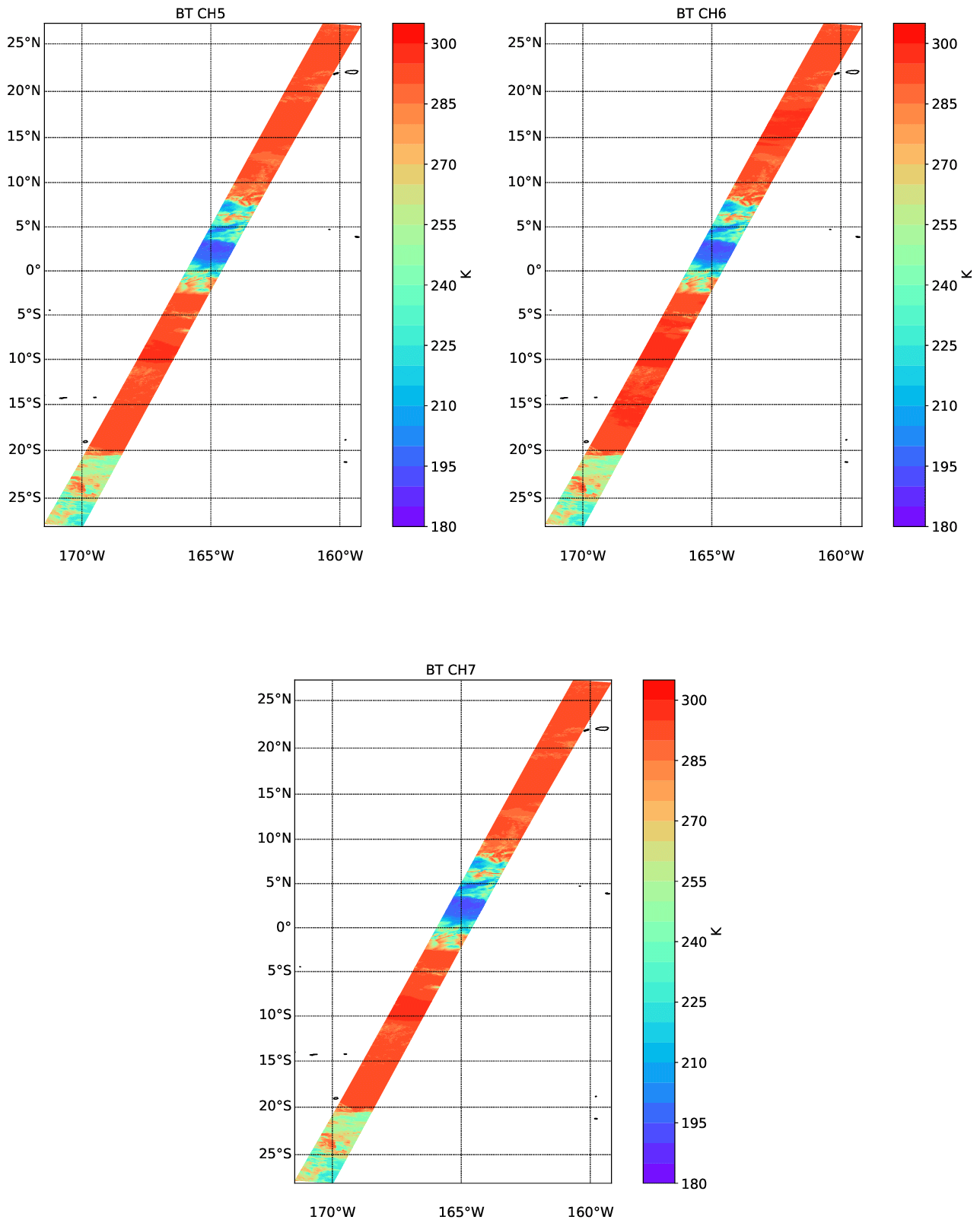
Figure 31 Simulated TOA brightness temperatures for the three LW EarthCARE MSI channels for the Hawaii scene.

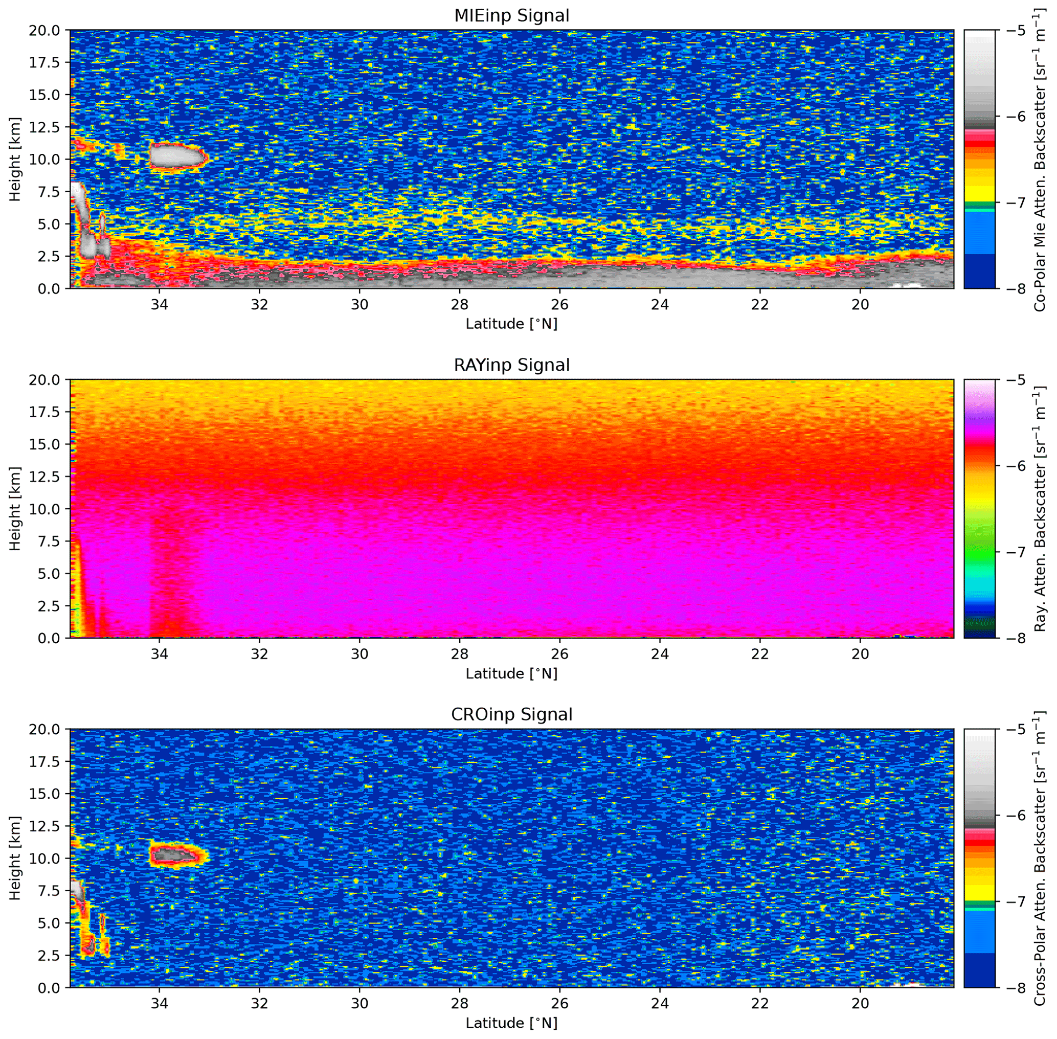
Figure 32 Simulated Mie channel, Rayleigh channel, and cross-polar ATLID attenuated backscatters for the Halifax aerosol scene.

3.4 Halifax aerosol scene

As a last test scene based on GEM and CAMS inputs and used in the processor development within this special issue, a mainly aerosol scene was built from a subsection of the Halifax scene. For this “Halifax aerosol” scene the region south of 36^∘ N was used; however, all liquid clouds and aerosol types were removed except for the coarse-mode non-absorbing aerosol (sea salt). The remaining aerosol particle density was scaled by a factor of 2 to increase the total optical thickness and detectability by the MSI instrument. The resulting scene contains ice cloud north of about 33^∘ N and an aerosol-rich boundary layer marine aerosol layer limited to an altitude of about 2.5 km with a very tenuous layer above. The lidar-observed attenuated backscatter fields are shown in Fig. 32, while the MSI images are shown in Figs. 33–35.

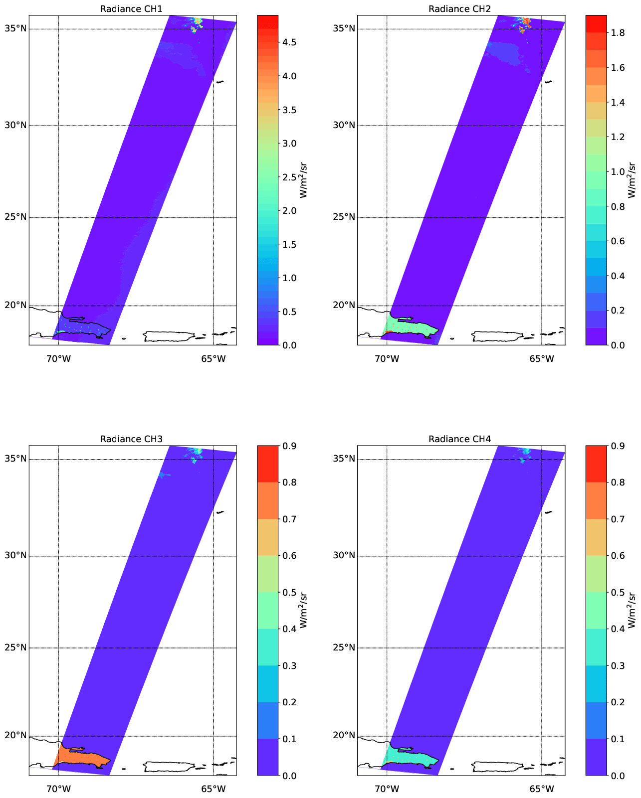
Figure 33 Simulated TOA radiances for the four SW EarthCARE MSI channels for the Halifax aerosol scene.

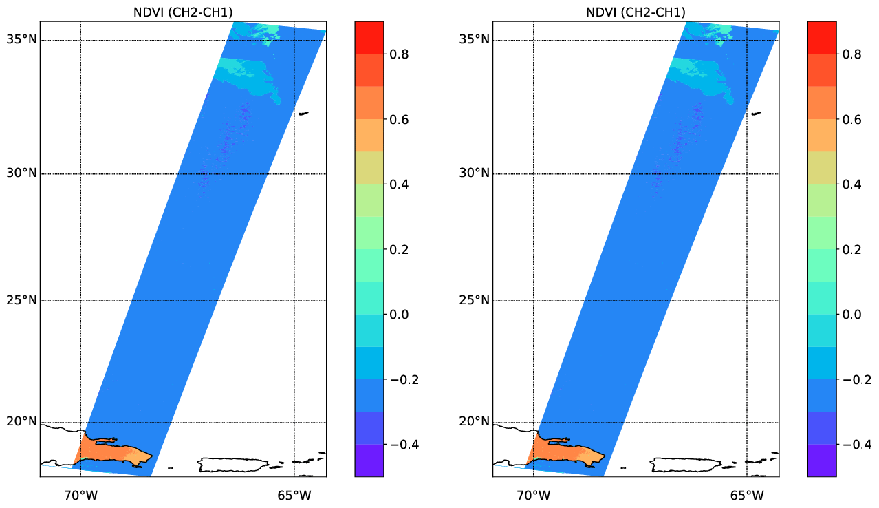
Figure 34 NDVI values corresponding to the simulated radiances shown in Fig. 33.

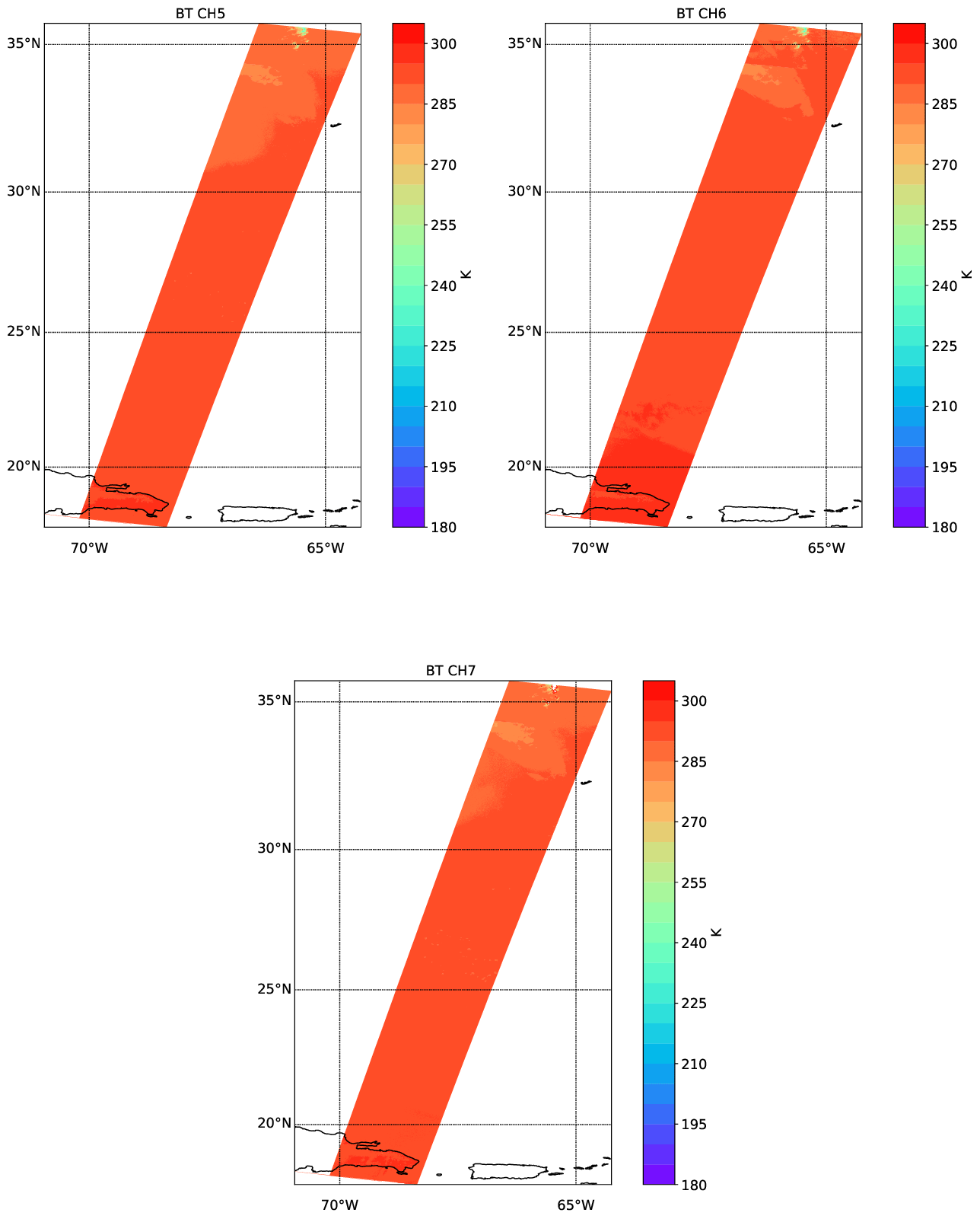
Figure 35 Simulated TOA brightness temperatures for the three LW EarthCARE MSI channels for the Hawaii scene.

4 Conclusion

In this paper the main testing and development scenes used for EarthCARE L2 algorithm scientific and technical development and testing have been presented. The model data used as the basis for the scenes are discussed in a companion paper (Qu et al., 2022). The focus of this paper has been to present the modeled L1 signals for each of the EarthCARE instruments and to document the methods used in their creation. The L1 signals, together with the corresponding model truth field, have in turn been used to develop a suite of single- and multi-instrument retrieval processors. These processors are described by various companion papers. Further insight into the expected precision, accuracy, and coverage of the EarthCARE data can be found in an algorithm inter-comparison paper (Mason et al., 2023).

Numerous other studies, beyond what has been presented within this special issue, could be conducted using this simulated data set. Post-launch, the simulations presented here will continue to play a role in the evolution of the various processors. Post-launch activities, including investigating the effects of in-orbit EarthCARE instrument degradation, may be conducted using the present simulations as a base. In addition, the simulations could be expanded to include other past instruments, e.g., CALIPSO, or future proposed lidars or radars. Such activities may be useful in understanding the relationship between, for example, the existing CALIPSO aerosol record and expected EarthCARE results.

The detail, realism, physical consistency, and scale of the test scenes developed for EarthCARE algorithm development, implementation, and testing comprise a unique effort. The creation of detailed realistic test scenes has involved considerable work but should be judged as time well spent. Not only have they served to develop new scientific inversion approaches, but they have also proved very useful in terms of technical development. It is true that the success of any inversion procedure must be evaluated using real data; however, the ability to compare against a “model truth” is invaluable when constructing new inversion algorithms, both in a scientific sense and in a technical (e.g., debugging) sense.

When actual EarthCARE data are available, there will no doubt be surprises to be dealt with. The extensive algorithm development process, aided by the simulations, will help ensure that these unexpected issues will be handled efficiently.