Observation of horizontal temperature variations by a spatial heterodyne interferometer using single-sided interferograms

Analyses of the mesosphere and lower thermosphere suffer from a lack of global measurements. This is problematic because this region has a complex dynamic structure, with gravity waves playing an important role. A limb-sounding spatial heterodyne interferometer (SHI) was developed to obtain atmospheric temperature retrieved from the O₂ A-band emission, which can be used to derive gravity wave parameters in this region. The 2-D spatial distribution of the atmospheric scene is captured by a focal plane array. The SHI superimposes the spectral information onto the horizontal axis across the line-of-sight (LOS). In the usual case, the instrument exploits the horizontal axis to obtain spectral information and uses the vertical axis to get spatial information, i.e. temperature observations at the corresponding tangent points. This results in a finely resolved 1-D vertical atmospheric temperature profile. However, this method does not make use of the horizontal across-LOS information contained in the data.

In this paper a new processing method is investigated, which uses single-sided interferograms to gain horizontal across-LOS information about the observed temperature field. Hereby, the interferogram is split, and each side is mirrored at the centre of the horizontal axis. Each side can then be used to retrieve an individual 1-D temperature profile. The location of the two retrieved temperature profiles is analysed using prescribed horizontal temperature variations, as it is needed for deriving wave parameters. We show that it is feasible to derive two independent temperature profiles, which however will increase the requirements of an accurate calibration and processing.

1 Introduction

The dynamical structure of the mesosphere and lower thermosphere (MLT) is mainly driven by atmospheric waves like planetary waves, tides, and gravity waves (Vincent, 2015). Gravity waves are small-to-medium-scale wave patterns, which transport energy from lower altitudes to the MLT region. Commonly known sources of gravity waves in the lower atmosphere are the uplift of air masses due to orography, convection, and unstable jets. Alexander et al. (2010) summarized the current treatment of gravity waves in global circulation models, where unresolved gravity waves are mostly parameterized. Becker and Vadas (2020) pointed out that gravity waves can also have sources in higher altitudes which are not well understood but can have a large effect on the MLT region. Chen et al. (2022) underlined the importance of gravity wave observations by multiple examples and outlined an observation method where gravity wave parameters can be extracted from temperature fields.

Temperature in the MLT region can be derived by measuring the O₂(0,0) atmospheric A-band emissions at 762 nm as shown by Ortland et al. (1998) and Sheese (2009). The same atmospheric band was used by the Michelson Interferometer for Global High-resolution Thermospheric Imaging (MIGHTI) instrument on board the NASA Ionospheric Connection Explorer (ICON) (Englert et al., 2017). MIGHTI uses three narrow spectral regions within the oxygen A-band to derive the temperature product. Notably, large-scale gravity waves have been detected through measurements taken in 2020, as reported by Triplett et al. (2023). Additionally, the Swedish MATS (Mesospheric Airglow/Aerosol Tomography and Spectroscopy) satellite mission employs two band regions within the oxygen A-band to extract temperature information, and the potential application of these data for gravity wave observations is explored in a simulation study by Gumbel et al. (2020). Both MIGHTI and MATS employ multichannel photometric measurements.

Simultaneously, a collaborative effort between the Jülich Research Center and the University of Wuppertal in Germany led to the development of a limb-sounding spatial heterodyne interferometer (SHI) for deriving temperature in the MLT from the oxygen A-band emission (Kaufmann et al., 2018; Song et al., 2017). This instrument employs interferometry, enabling the resolution of individual emissions within the oxygen A-band. After a successful in-orbit demonstration of the measurement technology in 2018, an improved second version, called AtmoLITE, was developed and built for the International Satellite Program in Research and Education (INSPIRE). Additionally, the European Commission has selected this instrument for in-orbit validation as part of its H2020 programme. Details of the AtmoLITE instrument design are partially covered by Chen et al. (2022) and will be described further in Sects. 2 and 3.1.

The temperature is derived from the relative intensities of the O₂ (0,0) atmospheric A-band emission lines. Consequently, no absolute radiometric calibration is required, simplifying the calibration process. Notably, these emissions are visible both during daytime and nighttime. The instrument is highly miniaturized and energy efficient so that it can fly on nanosatellites, so-called CubeSats (Poghosyan and Golkar, 2017). CubeSats allow for a cost-efficient way to design and operate satellites due to the utilization of largely standardized components.

The AtmoLITE instrument works as a camera where the atmospheric scene is mapped onto the detector. The SHI superimposes the spectral information of the O₂ A-band emission in the horizontal direction across the LOS. Each image thus contains superimposed spectral and spatial information along the horizontal axis while preserving spatial information vertically. In the usual processing, spectral information is extracted from the horizontal axis, and spatial information is derived from the vertical axis. This approach enables the extraction of finely resolved 1-D temperature profiles with an intended vertical resolution of 1.5 km from a single image. The resulting temperature profiles can then be used to derive wave parameters, as outlined by Ern (2004) and adapted for the AtmoLITE instrument by Chen et al. (2022). This capability allows AtmoLITE to effectively capture and analyse vertically propagating gravity waves of small-to-medium scale.

To exploit some of the spatial information in the horizontal direction, we propose a new processing method which allows users to retrieve two 1-D temperature profiles from one image by using single-sided interferograms and mirroring them at the centre. Johnson et al. (1996) and Gisi et al. (2012) already used mirrored interferograms for the far-infrared spectrometer (FIRS)-2 and for the TCCON FTIR spectrometer, respectively, to achieve a higher spectral resolution. In our case, we use the single-sided interferogram to gain horizontal information of the measured atmospheric scene. Chen et al. (2022) showed in a simulation study that medium-scale gravity waves can be resolved if it is possible to obtain two temperature profiles from a single interferogram. The methodology to fulfil this requirement is described in this paper.

A thorough precision analysis is key to assess the limitations of this method. Therefore we detail the precision budget of the data product, in particular with regard to signal-to-noise limitations at the upper boundary of the measurement domain.

The paper is structured as follows. We introduce the instrument in Sect. 2. An overview of the simulation set-up is given in Sect. 3, containing the interferogram simulation presented in Sect. 3.1, followed by the detailed forward simulation in Sect. 3.2 and the data processing in Sect. 3.3. The temperature dependency of the emission lines and the resulting temperature precision are discussed in Sect. 4. An extended discussion on using half interferograms is given in Sect. 5. Hereby, we look at the temperature sensitivity of the retrieval with respect to the temperature variation in the horizontal direction in Sect. 5.1. Further, we assess the locations of the retrieved temperatures using half interferograms for simulated horizontal temperature variations in Sect. 5.2. At last we assess the effect of apodization onto the retrieval using half interferograms in Sect. 5.3.

2 Spatial heterodyne interferometer

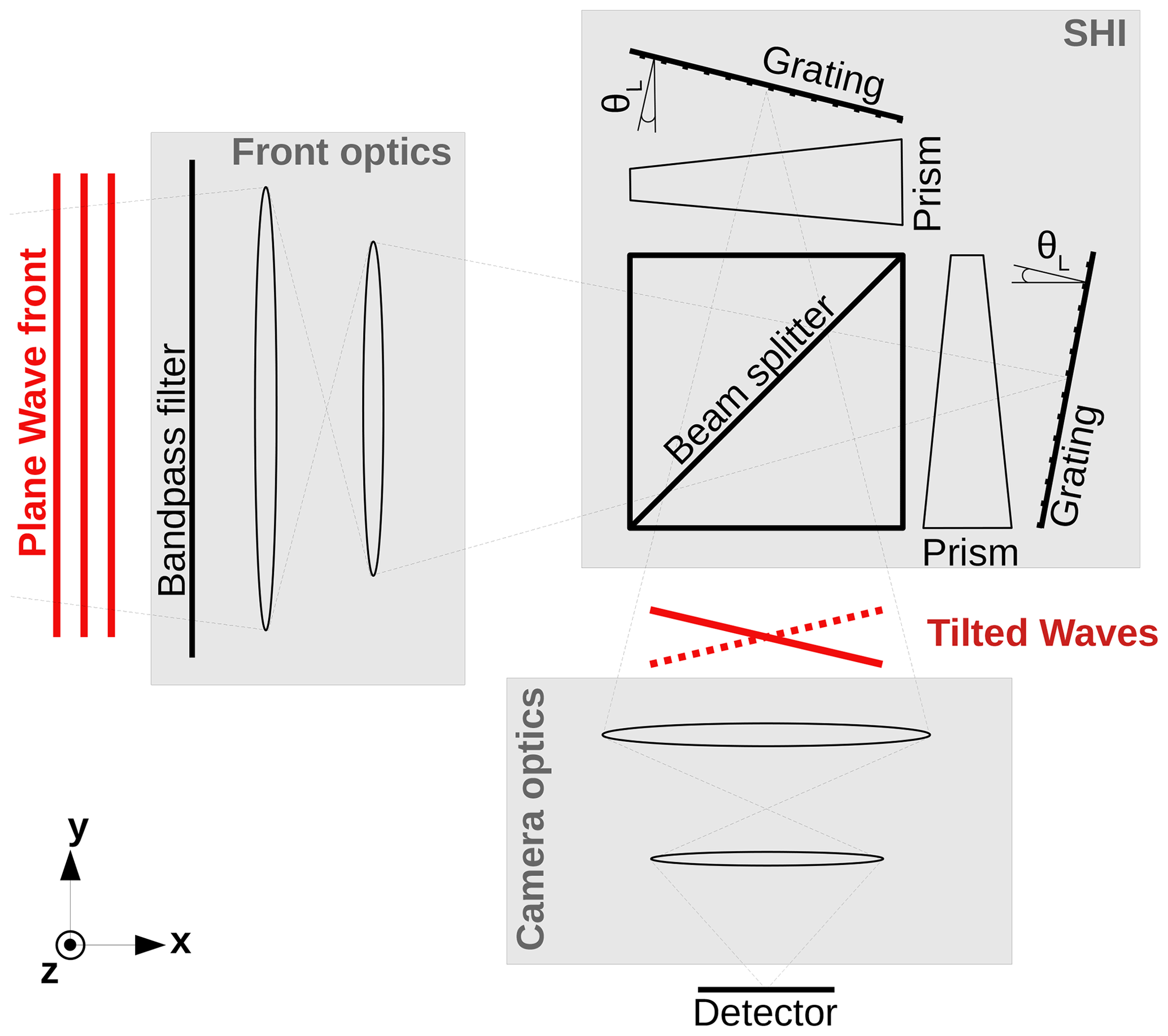
A spatial heterodyne interferometer (SHI) is similar to a Michelson interferometer, but the two mirrors are replaced by fixed tilted gratings. This measurement method was firstly developed by Connes (1958), and with the subsequent availability of imaging detectors, it was further developed to remote sensing methods by, for example, Harlander et al. (1992), Cardon et al. (2003), and Watchorn et al. (2001). Figure 1 shows a schematic of the instrument. The incident light is imaged by the front optics onto diffraction gratings, after passing through a beam splitter. The camera optics images the gratings onto a two-dimensional focal plane array (FPA). The tilt angle of the wave fronts and therefore the frequency of the interference pattern on the FPA are dependent on the frequency of the incoming light. Multiple emission lines result in superimposed cosine waves across the FPA in the x direction. The FPA is two dimensional, so the spatial distribution of the atmospheric scene is maintained throughout the instrument. One measurement therefore contains spatial information along the z axis with superimposed spectral and spatial information along the x axis. Note that the z and x axes correspond to the vertical and horizontal across-track dimensions in the atmosphere.

Figure 1 Schematic of the SHI instrument.

3 Simulation set-up

An interferogram simulation is presented in Sect. 3.1. The details of the forward simulation to calculate the expected signal is introduced in Sect. 3.2. At last the data processing is described in Sect. 3.3.

3.1 Interferogram simulation

The mathematical derivation for an interferogram measured by an SHI is presented by Harlander et al. (1992), Smith and Harlander (1999), and Cooke et al. (1999). Chen et al. (2022) give more details on the mathematics for the instrument described here.

A line-by-line model is used to simulate spectra which are converted to interferograms. A 1-D interferogram with some horizontal variation is defined by

$$\begin{array}{}\text{(1)}& I\left(x\right)=\sum _{i=\mathrm{1}}^I{S}_i\left(x\right)\left[\mathrm{1}+\cos \left(\mathrm{2}\mathit{\pi }{f}_{i}x\right)\right],\end{array}$$

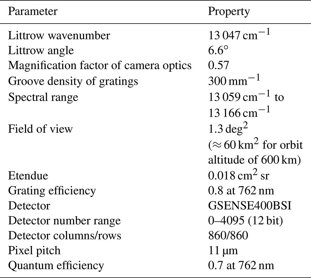
where S_i(x) is the radiance variation across the horizontal field of view, and f_i is the spatial frequency for a given emission line i. The spatial frequency corresponds to the wavenumber by $f_i=\mathrm{4}({\mathit{\sigma }}_i-{\mathit{\sigma }}_L)\tan {\mathit{\theta }}_{L}M$, where σ_L and θ_L are the Littrow wavenumber and Littrow angle, respectively. The Littrow angle is the tilt of the gratings as shown in Fig. 1. Note that the Littrow wavenumber corresponds to zero spatial frequency. M is the magnification factor of the camera optics, and σ_i is the wavenumber of the emission line. This instrument uses a CMOS-based detector, where shot noise dominates the precision of the data (Liu et al., 2019). Shot noise can be described by a Poisson process with mean and variance equal to the signal. For the expected signal levels, this can be approximated by an additive white Gaussian noise with standard deviation equal to the square root of the signal in each pixel. The specification of the current instrument version is given in Table 1.

Table 1 Summary of instrument specifications.

3.2 Detailed forward simulation

This section introduces shortly the simulation of the O₂ A-band emission, which is described by Chen et al. (2022) in detail. The O₂ A-band is an electronic transition from the excited state O${}_{\mathrm{2}}(b^{\mathrm{1}}{\mathrm{\Sigma }}_{\mathrm{g}}^{+}$, v=0) to the ground state O${}_{\mathrm{2}}(X^{\mathrm{3}}{\mathrm{\Sigma }}_{\mathrm{g}}^{-}$, v=0) centred at 762 nm in the near-infrared. The band consists of multiple emission lines due to the transition of multiple rotational states. In order to calculate the emission energies between the rotational states, the HITRAN database can be used (Gordon et al., 2022). The photo-chemical processes producing the excited O₂(¹Σ) molecules can be placed into three groups. The first group is the absorption in the B-band and the A-band itself. The second group produces excited O₂(¹Σ) molecules via collisional energy transfer with highly excited molecules and atoms produced by photolysis of O₂ and O₃. The third is called the Barth process and is a purely chemical source, which was first described by Barth and Hildebrandt (1961). It is independent of solar radiation, and it is therefore the only process active during nighttime. A detailed description of the dayglow O₂ A-band excitation is given by Sheese (2009), Bucholtz et al. (1986), Zarboo et al. (2018), and Yankovsky and Vorobeva (2020).

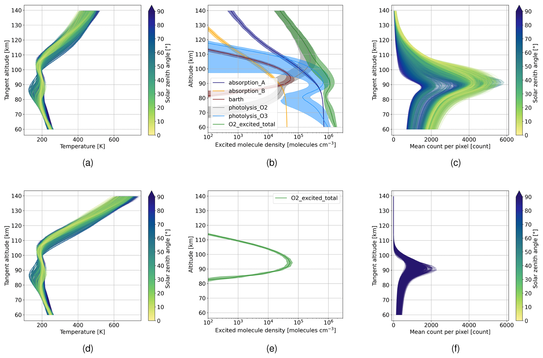
Figure 2 Panels (a) and (d) show 1-D input temperature profiles used in the forward calculation for solar minimum and maximum conditions, respectively; (b) number density of excited O₂ molecules due to the five production mechanisms during daytime condition; total excited O₂ is the sum of the five parts; (e) number density of excited O₂ molecules during nighttime condition, where only the Barth process is active; panels (c) and (f) show estimated count per pixel received at the detector during daytime and nighttime simulation, where the integration time is set to 1 and 10 s, respectively; the HAMMONIA data set is used for the forward simulations (Schmidt et al., 2006).

To calculate the O₂ A-band volume emission rates, data of the HAMMONIA (Hamburg Model of the Neutral and Ionized Atmosphere) run of Schmidt et al. (2006) are used. They give monthly averaged 3-D data sets for temperature, pressure, and the volume mixing ratios of the required substitutes involved in the photo-chemical processes for solar minimum and maximum conditions. The overall description of the used one-dimensional radiative transfer model is described by Chen et al. (2022). The model is used to generate test data sets to be used in the following study, covering a equidistant longitude and latitude grid of 10^∘. At each longitude and latitude point, the solar zenith angle is calculated by assigning the timestamp to noon at the 15th of each month. This is done for each month and for solar minimum and maximum conditions. The expected mean signal per pixel at the detector can be calculated by

$$\begin{array}{}\text{(2)}& S_{\mathrm{p}}\left(z\right)={\displaystyle \frac{S_{\mathrm{r}}\left(z\right)EL{t}_{\mathrm{int}}}{N}},\end{array}$$

where S_r is the spectrally integrated radiation within the spectral range of the instrument for a given tangent altitude z, E represents the etendue of the instrument, L represents the loss factor or efficiency of the instrument (28 % including grating efficiency, quantum efficiency of the detector and loss of 50 % due to the beam splitter), t_int represents the integration time, and N represents the total number of pixels of the 2-D detector array. Figure 2a and d display the input temperature profiles for solar minimum and solar maximum conditions, respectively. The panels illustrate noticeable temperature deviations above 120 km between the two groups. Based on the temperature profiles, Fig. 2b and e show the mean and standard deviation of the expected number density of excited O₂ molecules due to the different production mechanisms for daytime and nighttime simulations, respectively. It should be noted that the Barth-process is the only active process during nighttime conditions. Propagating this through the radiative transfer model and applying Eq. (2), where we assume 1 and 10 s for daytime and nighttime, we can calculate the average count per pixel measured by the detector. The results are shown in Fig. 2c and f for daytime and nighttime simulations. The nighttime simulations show a lower variability than the daytime simulations. This can be explained by the larger variation of the photolysis production mechanisms shown in Fig. 2b, which is mainly caused by the varying solar zenith angle. Note that during daytime the expected signal at the instrument decreases below 90 km, which can be partly explained by the decreasing number density of excited O₂ in Fig. 2b. However, for tangent altitudes below 85 km self-absorption plays a major role, leading to a further decrease in the signal at the instrument despite the increase in the number density of excited O₂. This constrains the information content of temperature data obtained from measurements of that region. The decreasing signal in higher altitudes above 120 km constraints the measurement method from above. Further discussion on the upper limit is given in Sect. 4. To neglect self-absorption in this paper, we will focus on a field of view between 80 and 140 km. Consequently, due to the self-absorption effect, the results for the lowermost tangent altitudes, below ≈85 km, need to be treated with reservation.

3.3 Fast data processing

The first step in the data processing is to subtract the non-modulated part, which corresponds to the low frequencies in the spectrum. By subsequently applying a Fourier transformation along the x axis, the interferogram is converted into a spectrum. A two-dimensional radiative transfer model is used to simulate across-track temperature variations. Assuming that self-absorption is small, we can focus on the area close to the tangent layer, where most of the information comes from when integrating along the line of sight. Note that this holds true for tangent altitudes above 85 km for the O₂ A-band emission. Furthermore, stray light is not included in this study, but it impacts daytime simulations, mainly tangent altitudes below 85 km due to upwelling radiation and above 120 km due to the low signal strength. A first assessment is presented by Kaufmann et al. (2023), and possible correction methods will be investigated in future research.

Since self-absorption is not considered in this study, a simplified forward model can be used to solve the inverse problem and retrieve temperature. Instead of calculating the full radiative transfer equation, it calculates the relative distribution of the oxygen A-band emission lines for a given temperature following Song et al. (2017), where the required spectroscopic parameters of the emission lines are taken from the HITRAN data set. Subsequently, it convolves the emissions with a given instrument line shape (ILS) and scales the total spectrum with a scaling factor to match the output spectrum from the Fourier transform. In this context, the factor corresponds to the number density of excited O₂(¹Σ) molecules. It is important to highlight that the atmospheric emission lines are very narrow, allowing us to approximate them as shifted Dirac delta distributions. When a function is convolved with a Dirac impulse, the result is the same function shifted by an amount equal to the shift of the Dirac impulse. Consequently, the ILS can be positioned at the location of the emission line, scaled by the line strength and summed up to obtain an analytical spectrum for a given temperature. By employing this approach in the retrieval process, we can effectively derive an averaged temperature from the horizontal temperature variation for a given tangent altitude.

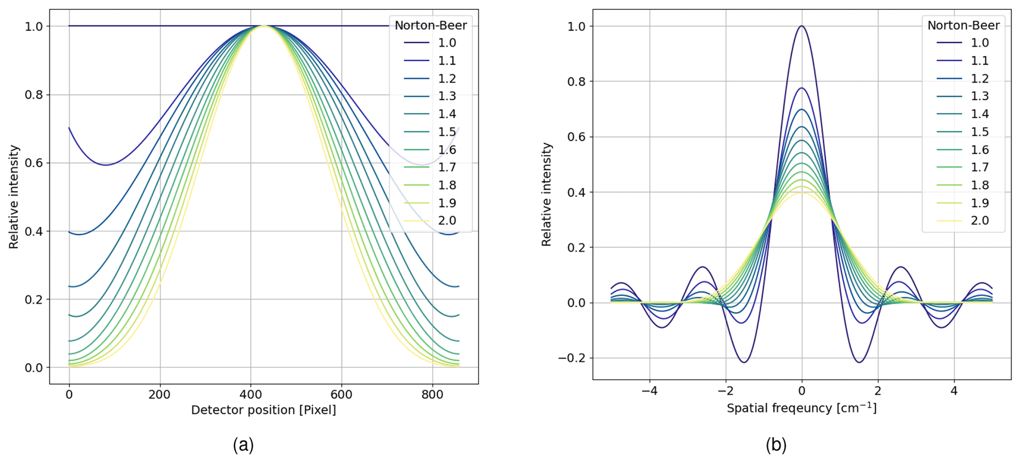
Figure 3 Apodization functions used for the assessment; (a) apodization function in the spatial domain; (b) apodization function in the spectral domain.

The ILS of a finite interferogram is defined by a sinc function whose resolution is determined by the length of the interferogram. To minimize the side lobes of the sinc function, apodization is commonly applied in Fourier spectrometry, resulting in a smoother spectral output. It increases the localization of the spectral information, which can also help to be more robust against instrumental errors. However, apodization decreases the spectral resolution, and it is therefore a trade-off between spectral resolution and a decrease of the side lobes. Filler (1964) introduced Filler's diagram, which plots these two measures against each other. It is often used to assess the performance of given apodization functions. Norton and Beer (1976) and Naylor and Tahic (2007) showed that the Norton–Beer apodization has the best properties. The extended version given by Naylor and Tahic (2007) is shown in Fig. 3 for the spatial and spectral domain. A value of 1.0 refers to no apodization, and 1.2, 1.4, and 1.6 refer to weak, medium, and strong apodization, respectively, given by Norton and Beer (1976). Note that the number refers to the full width half maximum (FWHM) of the apodization function relative to the sinc function and thus a higher number means stronger apodization.

4 Temperature dependency of the O₂ A-band emission

Our simplified forward model relies on the temperature-dependent rotational distribution of the O₂ A-band emission. The temperature dependency is shown in Fig. 4a. At low temperatures the central frequencies show higher intensities, which decrease to the sides. Higher temperatures show a more broadened distribution which entails a decrease of the integrated intensity within the bandpass filter. The gradient with respect to temperature decreases with higher temperatures, which entails a decrease in sensitivity towards higher temperatures. Convolving the emission lines with an instrument line shape (ILS), corresponding to a Norton–Beer strong apodization (Sect. 3.3), results in the spectra presented in Fig. 4b. Note the increase of the intensities at 13 165 cm⁻¹ due to the high density of emission lines in the R branch.

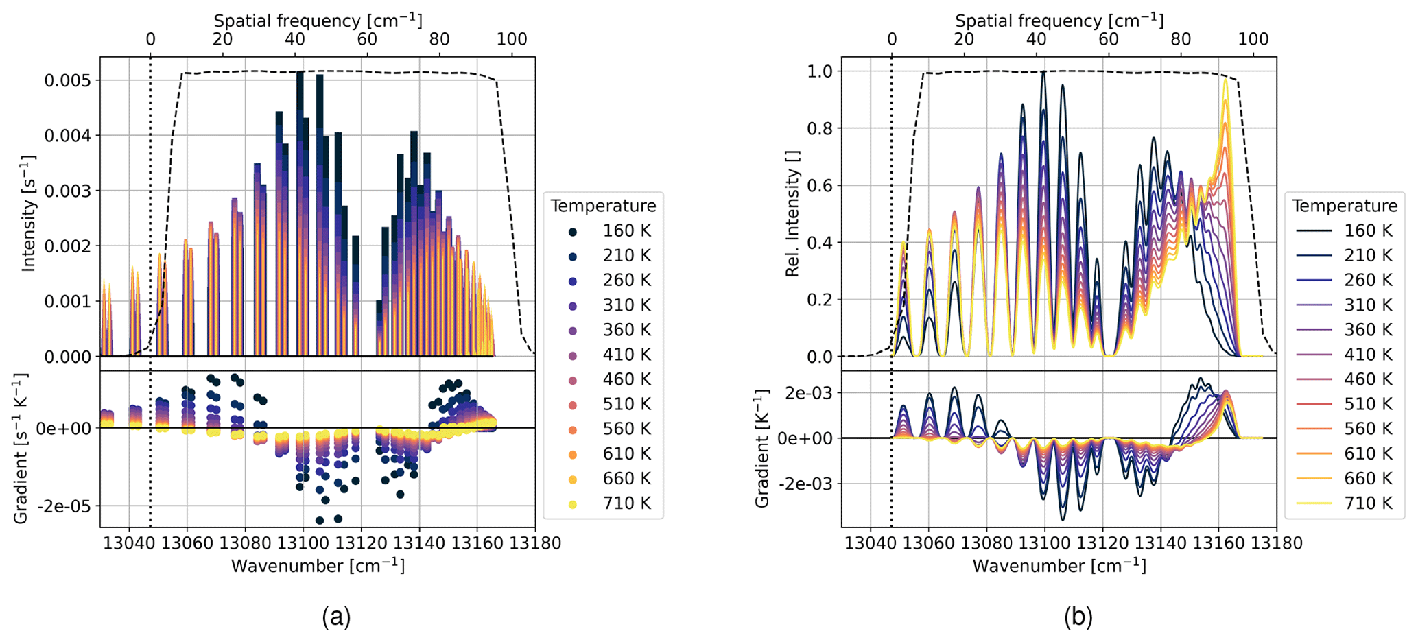
Figure 4 Rotational distribution of the O₂ A-band emission; the dashed and vertical dotted line indicate the curve of the bandpass filter and the Littrow wavenumber, respectively; the top x axis shows the spatial frequency at the detector; the gradient is calculated by finite difference along the temperature axis; (a) intensity of emission lines calculated using HITRAN for different temperatures; (b) convolution of emission lines with Norton–Beer strong ILS.

In the following, we propagate the shot noise in the interferogram through the simplified temperature retrieval for different signal levels and constant temperatures. For each signal level and temperature, we perform a Monte Carlo simulation with 300 samples, simulate an ideal interferogram using Eq. (1) for a given signal level and temperature, apply shot noise approximated by additive white Gaussian noise with variance equal to the signal level, and retrieve temperature as presented in Sect. 3.3. The signal level is expressed in the signal-to-noise ratio (SNR), which is the ratio of the mean to the standard deviation and thus the square root of the signal level itself. Figure 5 shows the bias and the standard deviation of the retrieved temperatures obtained in the Monte Carlo simulations. The top axis shows the mean signal, assuming that 20 rows are accumulated, which increases the SNR by a factor of $\sqrt{\mathrm{20}}$. The main reason for the binning is the limited data downlink capacity of microsatellites. A binning of 20 rows results in a vertical spatial sampling of approximately 1.5 km. The lower sensitivity of the O₂ A-band emission with higher temperatures is also visible here. For higher temperature, either a higher SNR is needed to keep the precision at the same level or one needs to accept a lower precision if SNR stays constant. The bias for low signals in Fig. 5a is caused by using magnitudinal spectra. When taking the absolute value of the spectrum, the spectral noise follows a Rice distribution (Talukdar and Lawing, 1991), which deviates from the normal distribution for spectral values close to zero. Therefore, low signals are affected more. More details on the spectral noise of a magnitudinal spectrum are given in Appendix A.

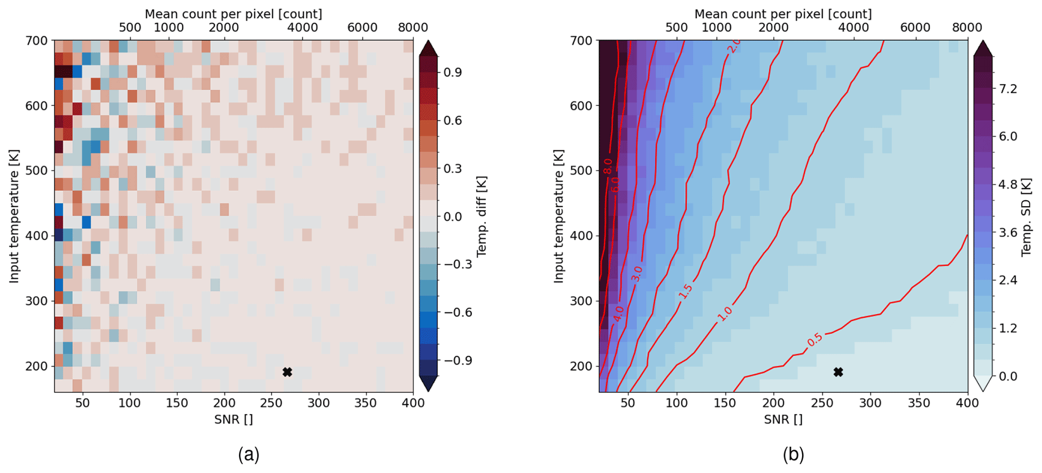
Figure 5 Results of the Monte Carlo simulations with 300 samples where shot noise is propagated into the temperature retrieval for different SNRs and temperatures; (a) mean temperature differences; (b) standard deviation of the retrieved temperatures; contour lines are calculated on smoothed data; the marker indicate the mean expected SNR and temperature in the mesopause region at 90 km altitude.

We then evaluate the interpolated temperature precision field presented in Fig. 5b on the expected signal levels (Fig. 2c and f) for typical temperature profiles in the MLT region (Fig. 2a and d). Hereby, we assume a binning of 20 rows. The results are shown in Fig. 6. The nighttime simulation gives a temperature precision below 1 K for tangent altitudes between 85 and 100 km. For the daytime simulation, a temperature precision of around 0.5 K can be achieved in the strong signal layer between 85 and 95 km. The temperature precision then decreases for higher tangent altitudes due to the decrease in signal and higher temperatures.

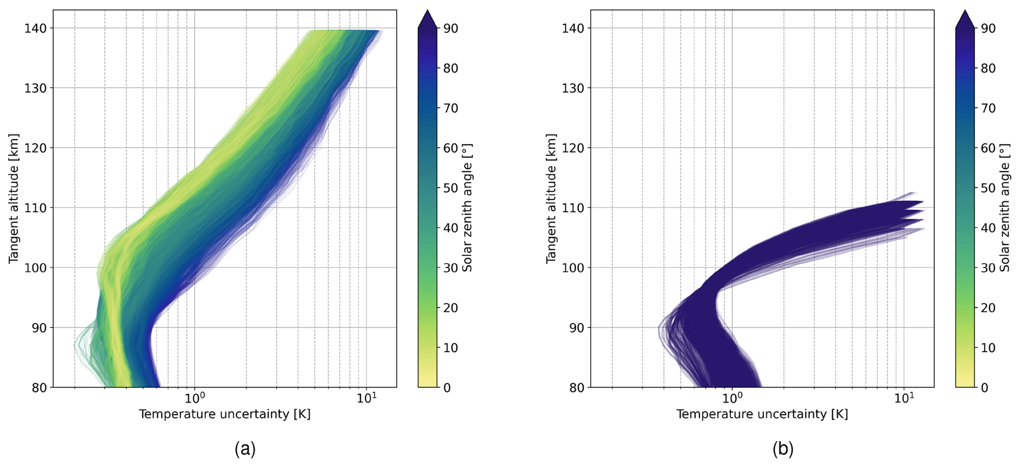
Figure 6 Temperature precision calculated from the expected signal and input temperature presented in Fig. 2 and using an interpolated temperature precision field presented in Fig. 5b, assuming a binning of 20 rows; panels (a) and (b) depict the day and nighttime conditions, respectively; note that signal counts below 100 are not considered, which cuts off the nighttime simulations around 110 km.

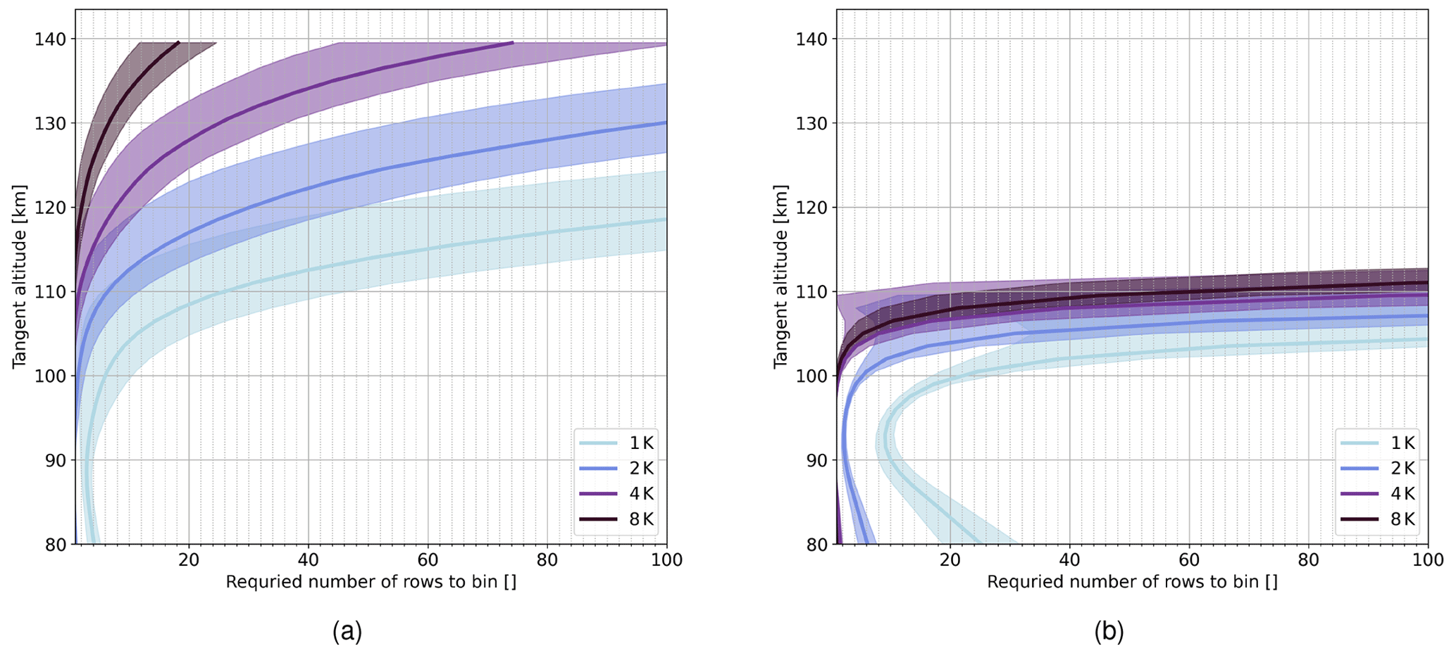
In the next step, we assess the required number of binning rows to achieve a certain temperature precision. Hereby, we extract a contour line from the temperature precision field in Fig. 5b, get the required signal for the temperatures presented in Fig.2a and d, and calculate the required binning using the expected signal in Fig. 2c and f for daytime and nighttime simulations, respectively. The results for different temperature precision levels are shown in Fig. 7. During daytime, we expect to resolve the higher altitudes on average up to approximately 105, 115, 125, and 135 km with temperature precisions of 1, 2, 4, and 8 K, respectively, when a binning of 20 rows is applied. During the nighttime simulation, accepting low temperature precision does not help to resolve higher altitudes because the signal decreases strongly above 100 km, as shown in Fig. 2f. In general, a larger binning can be applied to get more accurate results at the cost of spatial resolution, which is already proposed by Florczak et al. (2022). It is therefore a trade-off between spatial sampling and temperature precision.

Figure 7 Required binning of rows to achieve a certain temperature precision (a) during daytime and (b) during nighttime; the solid line shows the mean, and the shaded area shows the standard deviation of all used samples from Fig. 2c and f.

5 Obtaining horizontal spatial information by interferogram splitting

As explained in Sect. 2, the instrument contains the 2-D spatial distribution of temperature in its field of view. To gain more information, one can split the interferogram at the zero optical path difference (ZOPD). Exploiting the symmetry of the interferogram, each side is then mirrored around the ZOPD. This results in an interferogram of equal length as using the full interferogram, which then entails the same spectral resolution. When using the full interferogram, one half of the shot noise propagates into the real part and the other half into the imaginary part of the spectrum. Mirroring the interferogram, however, causes the shot noise to be symmetric so that it is then fully propagated into the real part of the spectrum, resulting in a higher noise level by a factor of $\sqrt{\mathrm{2}}$. To show this numerically, we perform a Monte Carlo simulation with 300 samples, where we simulate an interferogram using Eq. (1) for a constant temperature of 200 K across the horizontal field of view. The signal level is set to an SNR of 100, which results in a temperature precision of approximately 1 K as seen in Fig. 5b. Figure 8a shows the mean and the standard deviation of the interferogram samples. In the following step, we run through the processing chain explained in Sect. 3.3, extract the spectral noise, and retrieve the temperature for each Monte Carlo sample. The results are shown in Fig. 8b. As a reference, we show the spectrum without noise. Further, we show the standard deviation of the noise of the 300 samples for the case using the full interferogram and the two cases using mirrored single-sided interferograms. As stated before, the noise level is higher by a factor of $\sqrt{\mathrm{2}}$ for the mirrored single-sided interferograms compared to the full interferogram. This results in a correspondingly increased temperature precision of 1.4 K. Note that normally the noise is evenly distributed in the spectrum. If the signal, however, is close to zero, the noisy signal can take positive and negative values. Considering only magnitudinal spectra, the negative values are mirrored, resulting in a smaller standard deviation. More discussion on this is given in Appendix A.

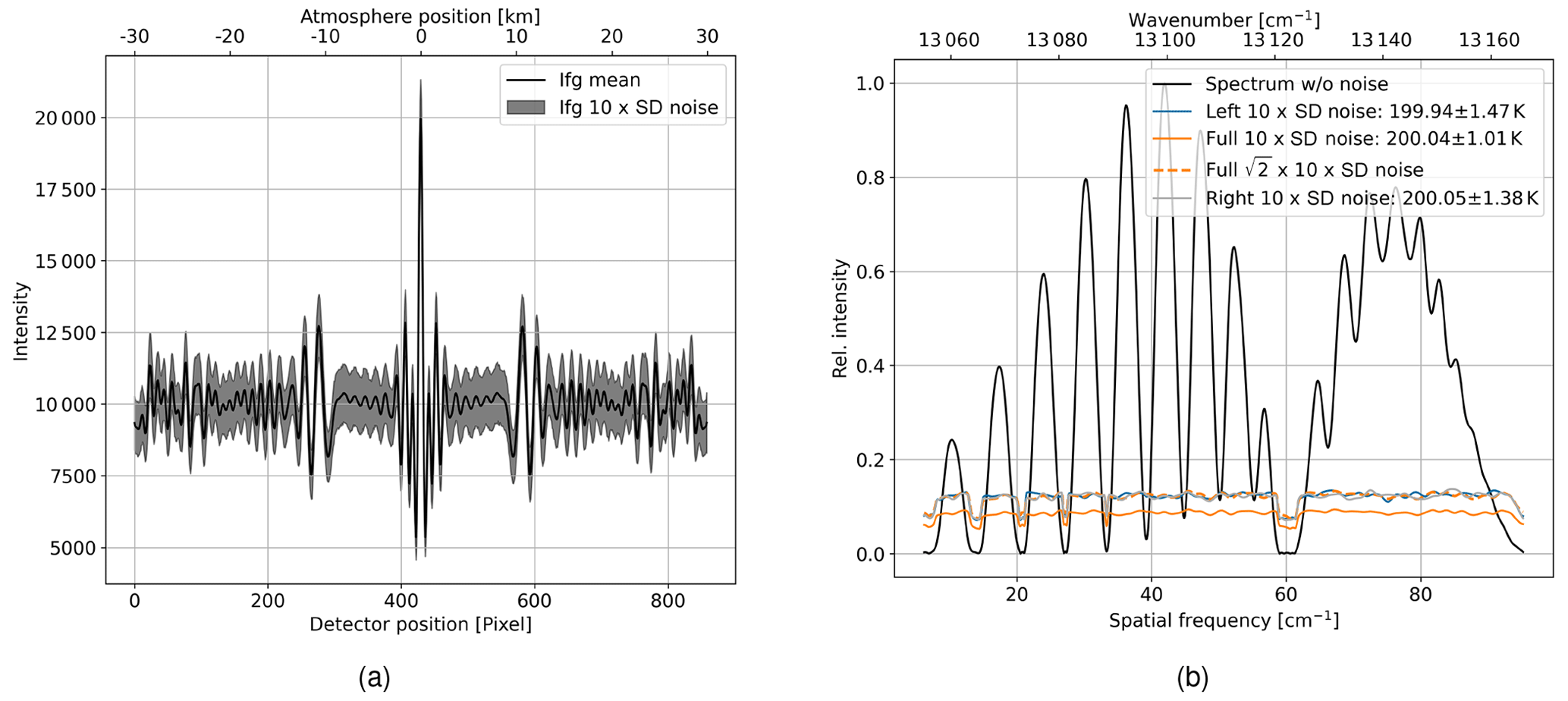
Figure 8 Results of Monte Carlo simulations with 300 samples where shot noise is propagated through the spectrum into the temperature retrieval for an interferogram with a constant temperature of 200 K; (a) mean and 10 times (10×) the standard deviation of the 300 interferogram samples; (b) spectrum without noise as a reference; 10× the standard deviation of the spectral noise using full interferograms and left- and right-side of the interferograms; standard deviation of the noise using the full interferograms multiplied by a factor of $\sqrt{\mathrm{2}}$ is shown as dashed line; Norton–Beer strong apodization is applied.

Performing the same analysis for multiple SNR and temperature levels gives the temperature precision of the right single-sided interferograms depicted in Fig. 9a. Figure 9b shows that for most temperature and SNR levels it holds true that the temperature precision is decreased by a factor of $\sqrt{\mathrm{2}}$ when using only the right single-sided interferogram. The same simulation has been performed for the left single-sided interferogram, and it showed a similar result. Thus, we can conclude that the increase of spectral noise by a factor of $\sqrt{\mathrm{2}}$ results in a decreases temperature precision by the same factor.

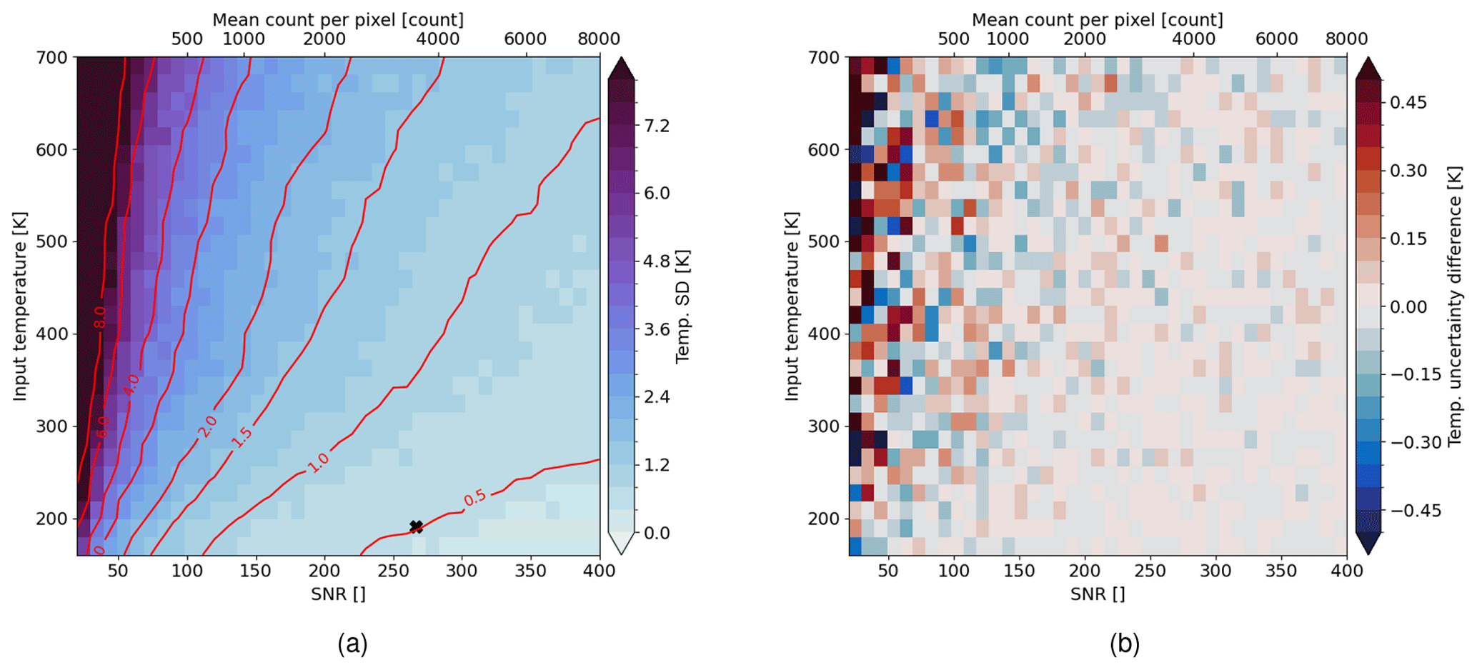
Figure 9 (a) Temperature precision of using the right single-sided interferograms assessed for different SNRs and temperatures; (b) difference of temperature precision using the right single-sided interferograms and temperature precision of full interferogram multiplied by $\sqrt{\mathrm{2}}$.

To study the influence of horizontal temperature variation on the temperature retrieval, we look at a simple example first. A linear temperature gradient of 20 K over the horizontal field of view of 60 km, shown in Fig. 10a, is incorporated into the interferogram by using Eq. (1). Figure 4a shows that for higher temperatures the integrated intensity within the bandpass filter decreases as the distribution of the emission lines becomes flatter. Following Eq. (1), the interferogram is just the sum of cosine waves with amplitude and offset equal to the intensity of the emission lines. The interferogram's baseline therefore also shows a decrease with higher temperatures, as shown in Fig. 10b. It shows an interferogram without noise and without temperature gradient as reference. We also show the difference between the interferogram with the linear temperature gradient and the reference interferogram relative to the mean signal of the reference interferogram. The linear regression of the difference agrees well with the relative variation of the integrated intensity within the bandpass filter. We perform a Monte Carlo simulation with 300 samples with shot noise modelled in the interferogram space. We run through the processing chain as explained in Sect. 3.3 to get a spectrum and a retrieved temperature for each sample. Note that the temperature gradient results in a tilted non-modulated part which is fitted and subtracted before splitting the interferogram. This is performed for the case using the full interferogram as well as the left- and right-mirrored interferograms, separately. Figure 10c shows the mean of all noisy spectra with constant temperature gradient as a reference. Furthermore, the smoothed mean difference of the noisy spectra incorporating the linear temperature gradient with respect to the reference spectrum is shown as well. Using the full interferogram, the mean difference shows only little differences across the spectral axis, which shows that the spectrum contains an averaged temperature information of the given temperatures within the field. Using only the left side of the interferogram entails that the interferogram contains only temperatures from 190 to 200 K. As explained in Sect. 4, lower temperatures means higher intensities in the central spectral region and lower intensities at the edges of the bandpass filter. Analogously, the same argument can be applied to the right side of the interferogram. The mean and standard deviation of the retrieved temperatures are shown in Fig. 10a. The precision of the temperature retrieval is again decreased by 0.3–0.4 K. Thus, the decrease in the temperature precision mainly comes from the mirrored shot noise. The retrieved temperatures of the single-sided interferograms lie on average 6 K apart from each other, which is closer than the mean temperature that each side suggests. The Fourier transformation maps a weighted sum of all spatial samples in the interferogram to a sample in the spectrum. Thus, the temperature information is localized in the interferogram but fully distributed across the spectrum. The retrieved temperature is therefore an average of the temperature information within a given region of interest in the interferogram. It should be noted that in the interferogram intensities that deviate significantly from the mean contribute more to the spectrum. Consequently, these deviations carry a greater amount of temperature information within the spectrum. Thus, the large variations around the ZOPD in the interferogram contribute more to the overall result. Equation (1) shows that the large variations comes from the fact that the interferogram consists of superimposed cosine waves with zero phase at ZOPD. This is the reason why we did not apply any apodization which applies higher weights to the central region of the interferogram. This will be discussed more in detail in Sect. 5.3.

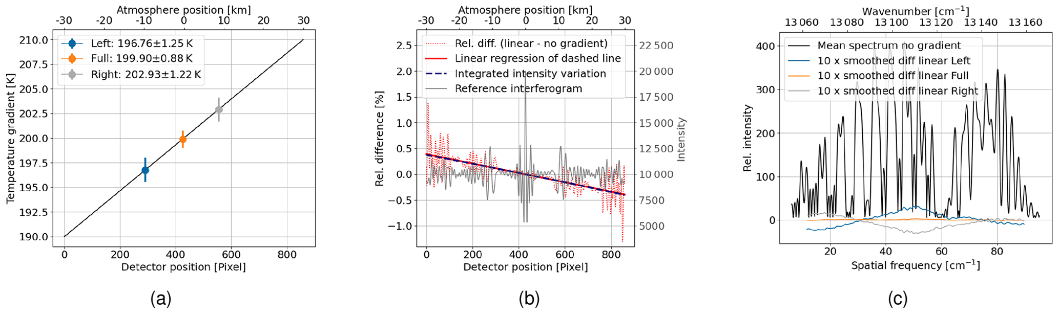
Figure 10 Results of Monte Carlo simulations with 300 samples where shot noise is propagated through the spectrum into the temperature retrieval for an interferogram with a constant temperature at 200 K and an interferogram with linear temperature gradient from 190 to 210 K; (a) used temperature gradient and retrieved temperatures; (b) reference interferogram (grey line, right y axis), incorporates a constant temperature at 200 K and a mean signal level of 10 000; difference between interferogram with linear temperature gradient and reference interferogram relative to the value 10 000 (mean of interferogram without temperature gradient), including the linear regression of the relative difference (red line, left y axis); integrated intensity variation within the bandpass filter due to the temperature gradient relative to the intensity corresponding to the central temperature of 200 K (blue line, left y axis); (c) mean of noisy spectra without temperature gradient as reference; mean difference between the noisy spectra incorporating the linear temperature gradient and the reference mean spectrum using full and half-sided interferograms; no apodization is applied.

It is important to acknowledge that the effectiveness of this method relies on accurate knowledge of the ZOPD location. Ntokas et al. (2022) conducted a sensitivity study to assess the impact of the ZOPD location and concluded that precise knowledge of the ZOPD on a sub-pixel scale is necessary to achieve the desired temperature accuracy and precision. Mirroring around the false ZOPD position increases all frequencies on one side and decreases all frequencies on the other side. Failure to account for this phenomenon during processing leads to inaccuracies in the temperature estimates. To accurately determine the ZOPD, correction techniques can be employed, which have already been applied to real-world data by Kleinert et al. (2014) and Ungermann et al. (2022). These methods effectively compensate for the interferogram shift by subtracting the linear phase from the spectrum.

5.1 Sensitivity to horizontal temperature variations

In this section we assess the sensitivity of the temperature retrieval to horizontal temperature variations. We define a function

$$\begin{array}{}\text{(3)}& f:\mathit{T}\mapsto T_{\mathrm{ret}},\end{array}$$

which maps the horizontal temperature variation T to a retrieved average temperature T_ret. We calculate the derivative of f with respect to T approximated by finite differences. Since the emission has different sensitivities at different background temperatures as shown in Fig. 4, the derivatives are calculated for the whole range of encountered temperatures. The result is shown in Fig. 11a. It shows an overall wavy pattern representing changing intensities of emission lines and its modulation through the instrument. The matrix shows that for any temperature level the retrieved temperature is most sensitive to temperatures close to the main lobe. Figure 11b shows smoothed rows for selected temperature levels of the matrix in Fig. 11a. Lower temperatures below 300 K show a lower sensitivity around the main lobe and more sensitivity to the side. Temperature levels around 500 K have the highest central peak and the lowest sides. This effect is attenuated for temperatures above 500 K. Thus, the temperature retrieval is least sensitive to horizontal temperature variations around 500 K. The same effect is seen in Sect. 5.2 and 5.3.

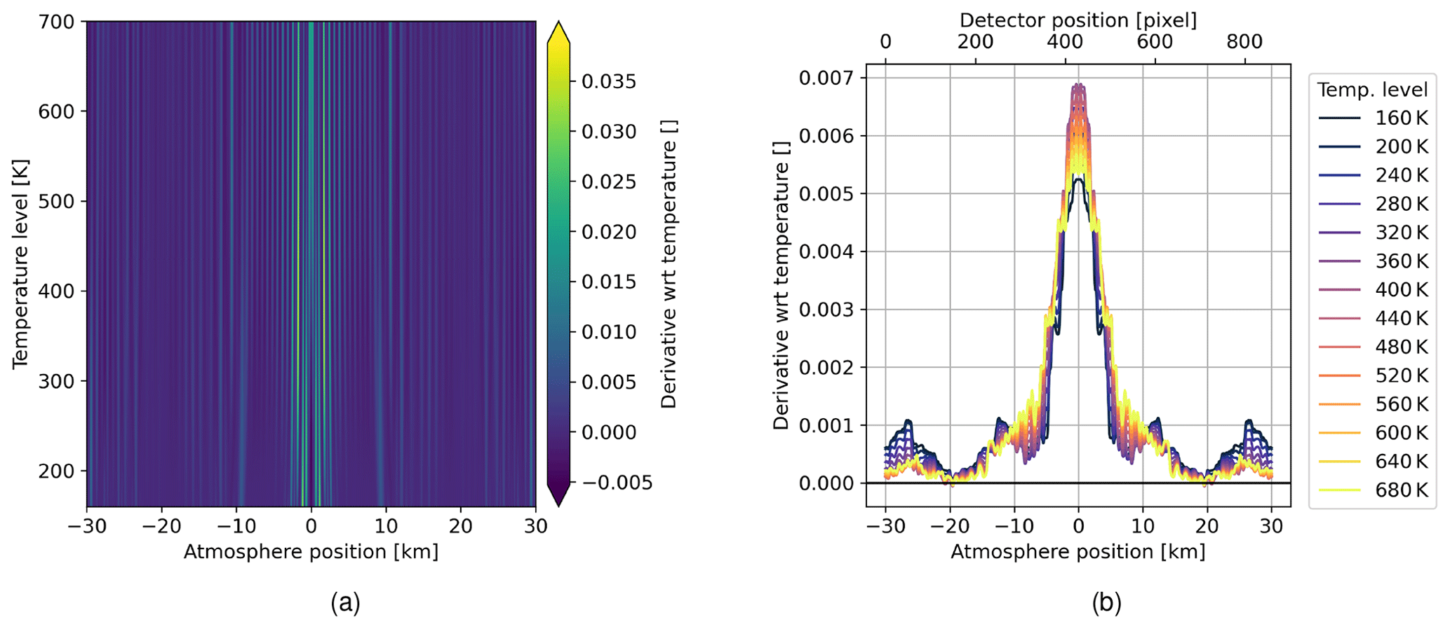
Figure 11 (a) Derivative of temperature at a given horizontal position for multiple temperature levels; (b) selected rows of (a) and smoothed by a running mean with window size of 101.

The Jacobian matrix in Fig. 11a can be used in Taylor's theorem to linearly approximate function f defined in Eq. (3). We interpolate the 2-D field and derive the continuous derivative with respect to temperature variation. We split the temperature variation in background and residuals, denoted by $\mathit{T}=\stackrel{\mathrm{‾}}{T}+{\mathit{T}}^{\mathbf{\prime }}$. The retrieved temperature can then be estimated due to Taylor's theorem by

$$\begin{array}{}\text{(4)}& {\stackrel{\mathrm{̃}}{T}}_{\mathrm{ret}}=\left(\mathrm{\nabla }f\left(\stackrel{\mathrm{‾}}{T}\right)\cdot {\mathit{T}}^{\mathbf{\prime }}\right)+\stackrel{\mathrm{‾}}{T},\end{array}$$

where ⋅ denotes the scalar product of two vectors. To put it into context with the linearized diagnostic theory described by Rodgers (2000), the Jacobian of function f is analogous to the averaging kernel matrix which also maps the atmospheric state to the retrieval result. The differences are that the function f maps a vector to a scalar and thus the Jacobian of f is a vector. Further, f and therefore its Jacobian are dependent on the background temperature. The functionality of the presented estimation, however, is similar to the usage of the averaging kernel matrix in a usual retrieval.

To evaluate this approximation, we use the simulated temperature variations from Sect. 5.2, estimate the retrieved temperature as explained, and compare it to the retrieved temperature running through the entire simulation-processing process explained in Sect. 3.2 and 3.3. The results are shown in Fig. 12, which shows an overall good agreement with 98 % being within an error of less than 0.05 K. A slight but negligible bias of 0.02 K can be seen. The minimal and maximal error is at −0.10 and 0.28 K, respectively. Thus, the explained method can be used to approximate the retrieved temperature for varying horizontal temperature variations without running through a full end-to-end simulation.

Figure 12 Temperature error using derivative matrix from Fig. 11a and Eq. (4) to estimate retrieved temperature.

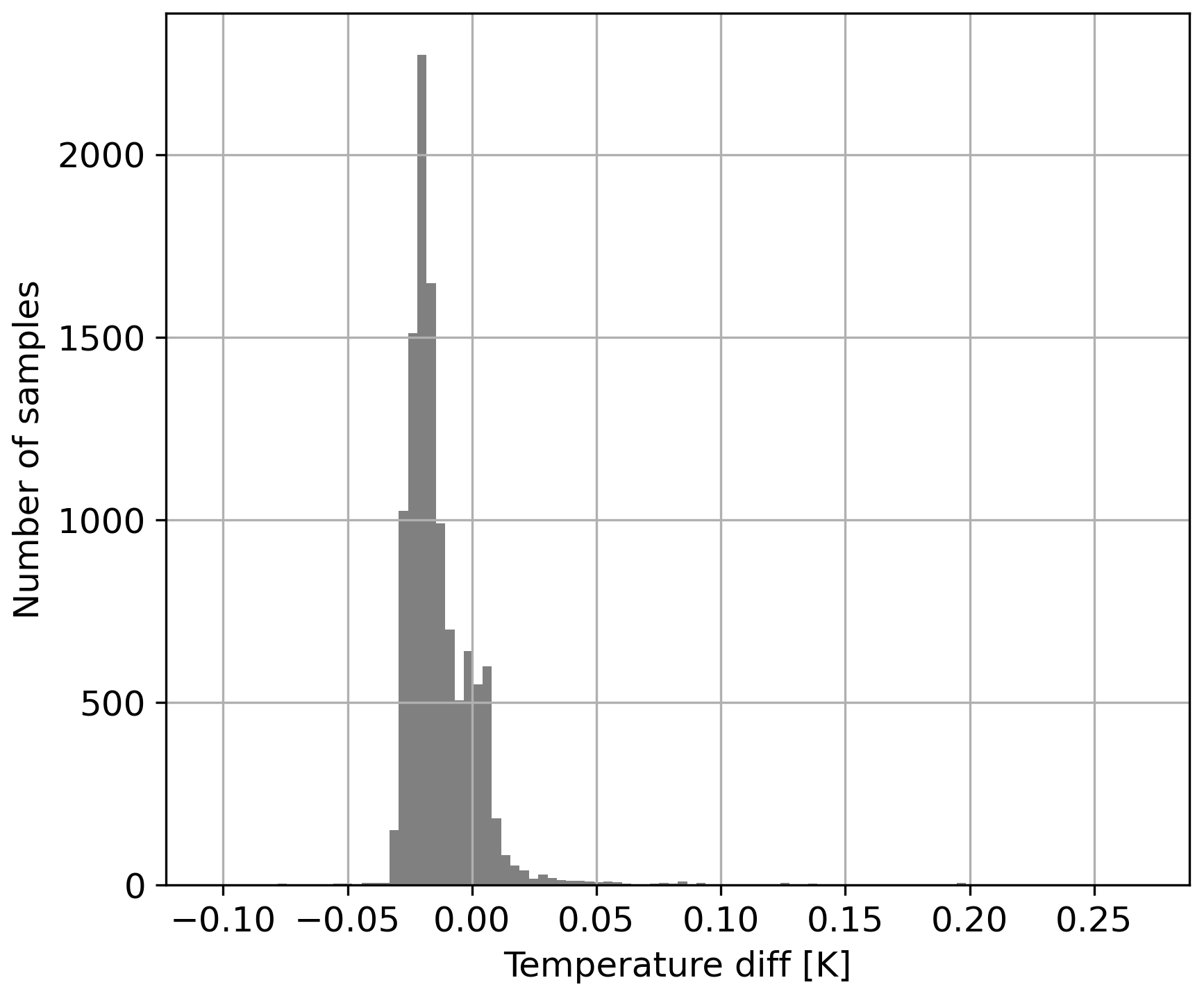
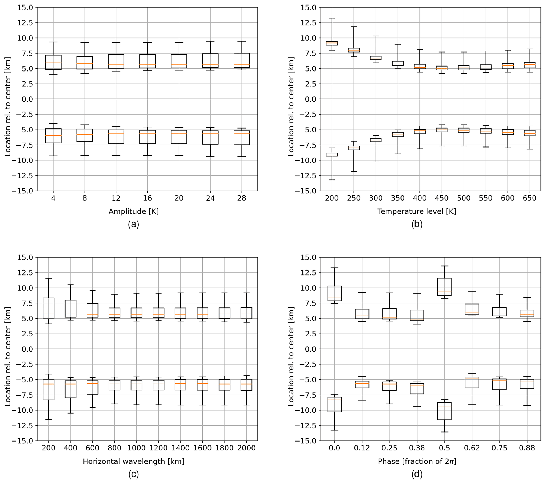
Figure 13 Relative location of the retrieved temperatures within the temperature variation using single-sided interferograms (a)  for varying amplitude, (b) for varying temperature background level, (c) for varying horizontal wavelength, and (d) for varying phase; the box extends from the lower to upper quartile values, and the whiskers extend from the 5th to 95th percentiles.

5.2 Temperature retrieval of horizontal temperature variations using single-sided interferograms

To get a comprehensive picture of the split interferogram processing method, we simulate interferograms according to temperature variations typically produced by gravity waves, split the interferogram, and retrieve temperature for each side. When observing temperature variations produced by an atmospheric wave, it is essential to localize that information in space to obtain proper wave characteristics from that data. A sinusoidal horizontal temperature variation can be modelled by

$$\begin{array}{}\text{(5)}& \mathit{T}=\stackrel{\mathrm{‾}}{T}+A\cos \left(\mathrm{2}\mathit{\pi }{\displaystyle \frac{\mathit{x}}{{\mathit{\lambda }}_h}}+\mathit{\varphi }\right),\end{array}$$

where $\stackrel{\mathrm{‾}}{T}$ represents the background temperature, A represents the amplitude, λ_h represents the horizontal wavelength, ϕ represents the phase, and x represents the horizontal scale. The horizontal field of view is assumed to be ± 30 km. Following Fig. 2a and d, we vary the temperature from 160 to 700 K to cover typical low- to mid-latitude conditions. Following Chen et al. (2022), we alter the horizontal wavelength from 200 to 2000 km and the amplitude from 4 to 30 K. In total, we analysed 4220 simulated temperature variations. Note that temperature variations with a min–max value smaller than 1 K are excluded, because they cannot be resolved. For further analysis, we introduce the term “location” of a retrieved temperature. This is defined by the abscissa of that atmospheric model temperature, which is equal to the retrieved one. The location of the retrieved temperatures of each side relative to the centre are shown in Fig. 13. Hereby, one parameter is varied while showing the distribution of all waves for the given parameter. Note that the distance between the locations of each side can be seen as a measure for how well the presence of a horizontal temperature variation can be characterized. Figure 13a shows no influence of the amplitude of the temperature residual on the location of the retrieved temperatures. Figure 13b shows that the temperature background affects the distance of the retrieved temperatures due to the different sensitivities of the O₂ A-band emission with respect to temperatures. The results in Sect. 5.1 explain the retrievals of lower temperature having a higher information content at the sides compared to that of higher temperatures and thus resulting in retrieved temperatures laying further apart from each other when using single-sided interferograms. The minimum of this effect is around 500 K, with a slight increase for temperatures above. The horizontal wavelength of the temperature variation only slightly affects the distance of the retrieved temperature as shown in Fig. 13c. Short wavelengths result in a larger spread of the location distribution due to the fact that the phase of the temperature variation plays a greater role. When looking at the phase in Fig. 13d, ϕ=0 and ϕ=π are outliers referring to the crest and trough of the captured temperature residual. In both cases, the temperature variation is low within the centre and large at the edges. This works against the increased temperature information around the centre and results in temperatures being further apart from each other. To conclude, if one takes the background temperature into account, one can give a good estimate of the location of the retrieved temperature. The effect of the phase will introduce a systematic error at the crest and trough. Compensating these two effects in the wave analysis, one gets a good estimate of the horizontal wave parameter components.

5.3 Apodization

In this section we assess the influence of apodization on the retrieval of split interferograms. We evaluate this for horizontally linear temperature gradients with a spread of ±10 K for central temperature levels from 160 to 700 K and for the Norton–Beer apodization introduced in Sect. 3.3. The results are shown in Fig. 14. Using the full interferogram, the mean temperature can be recovered for each temperature level independent of the strength of the apodization. Using a single-sided interferogram, stronger apodization decreases the localization difference between the retrieved temperatures of the left and right sides. Revisiting Fig. 3a, the apodization functions decrease the intensity of the interferogram towards the edges and thus put a greater weight on the information content in the central region. The effect that the retrieved temperatures are closer to the centre, as explained in Sect. 5.1, is consequently amplified by the apodization function. The case without apodization (Norton–Beer 1.0) shows a decrease in the temperature difference between the two sides for temperature levels between 160 and 500 K and a slight increase for higher temperatures. This shape is consistent with the results shown in Fig. 13b. When using mirrored single-sided interferograms, apodization is not only a trade-off between spectral resolution and decrease of the side lobes, but also a trade-off between spatial resolution of the two retrieved horizontal temperature data points and robustness against errors (see Sect. 3.3 for link between apodization and robustness). Using single-sided interferograms therefore increases the requirements for instrument error mitigation if the distance between the two retrieved temperature data points wants to be kept large.

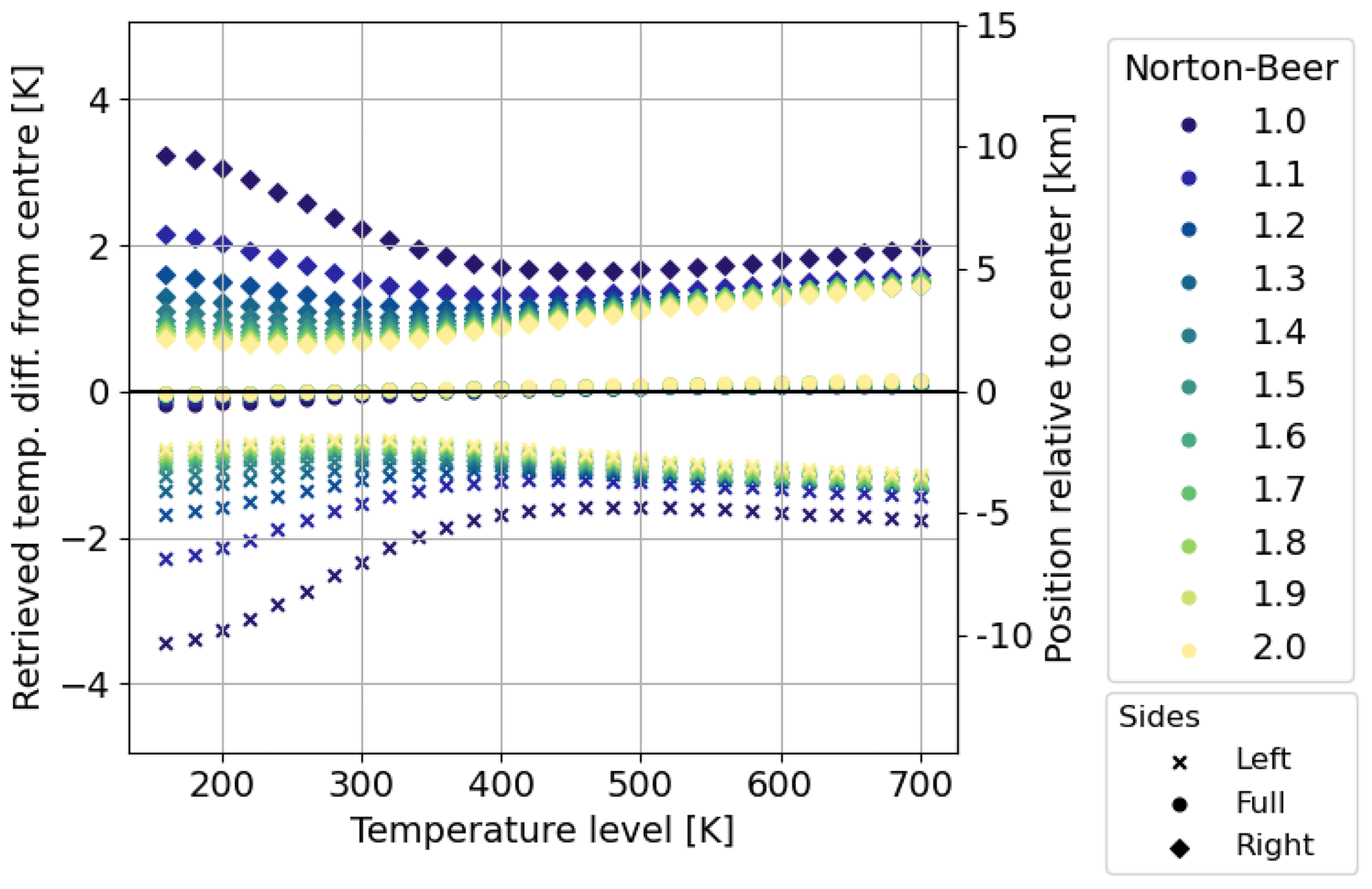
Figure 14 Retrieved temperatures using a linear temperature gradient for multiple temperature levels and different strengths of apodization

6 Conclusions

Spatial heterodyne interferometers are often combined with a two-dimensional focal plane array and a telescope to obtain spatial and spectral information from a scene. This study deals with a limb-sounding SHI instrument, which delivers in its default configuration spatial information of the atmosphere in the vertical and spectral information in the horizontal direction across the LOS. However, it is possible to split the interferogram into half to obtain additional spatial information in the horizontal direction across the LOS, as well. This methodology is firstly applied to spatial heterodyne spectroscopy for atmospheric temperature, which then gives two horizontal temperature profiles (two temperature data points per tangent layer).

This paper first discussed the temperature sensitivity of the captured O₂ A-band emission and the resulting temperature precision of the instrument. A special focus is put on the upper limit of resolvable tangent altitudes. To this end, we simulate the expected signal levels for the given instrument specifications and present a temperature precision analysis for different temperatures and signal levels using full interferograms as a baseline simulation. It was shown that the temperature precision is negatively correlated with temperature due to the specific temperature dependence of the emission lines, so thermospheric temperatures are less precise than mesospheric ones. The simulations show that within the strong emission layer around 90 km ± 10 km the temperature precision stays below 1 K. During daytime temperatures, altitudes up to 140 km can be resolved with either a lower temperature precision or a lower spatial resolution. For example, one would need to bin 60 rows to resolve tangent altitudes around 140 km with a temperature precision of 4 K. Our analysis does not account for self-absorption, which cannot be neglected for tangent altitudes below 85 km. To assess this effect, simulations using a radiative transfer model that includes self-absorption are required.

Further, we show that the method of split interferograms reduces the temperature precision by a factor of $\sqrt{\mathrm{2}}$. Analysing the influence of a horizontal temperature variation across the field of view shows that the horizontal localization of retrieved temperatures is generally closer to the centre of the field of view. A linearized estimation of the retrieved temperature for a given temperature variation using Taylor's theorem shows that most of the temperature information is localized around the centre of the interferogram. Further, it is shown that apodization affects the spatial resolution of the data obtained by this method. In general, weaker apodization gives better spatial resolution across the LOS, which must be balanced against model or instrumental uncertainties. As an application of this method, Chen et al. (2022) showed that medium-scale gravity waves can be horizontally resolved from such data, but it must be taken into account that the phase and background temperature of the captured wave affect the location of the retrieved temperatures.

Appendix A: Spectral noise of a magnitudinal spectrum

We can describe the noisy interferogram by

$$\begin{array}{}\text{(A1)}& \widehat{y}\left[n\right]=y\left[n\right]+\mathit{\epsilon }\left[n\right],\end{array}$$

where $\widehat{y}$ is the interferogram with noise, y the non-noisy interferogram, and ε the shot noise described by the normal distribution

$$\begin{array}{}\text{(A2)}& \mathit{\epsilon }\left[n\right]\sim \mathcal{N}(\mathrm{0},\stackrel{\mathrm{‾}}{y}),\end{array}$$

where $\stackrel{\mathrm{‾}}{y}$ is the mean of the signal.

The shot noise can be propagated through the Fourier transformation, resulting in a noisy spectrum given by

$$\begin{array}{}\text{(A3)}& {\displaystyle }\mathrm{Re}\left(\widehat{S}\right[k\left]\right)& {\displaystyle }\sim \mathcal{N}\left(S\left[k\right],{\displaystyle \frac{\stackrel{\mathrm{‾}}{y}}{\mathrm{2}N}}\right),\text{(A4)}& {\displaystyle }\mathrm{Im}\left(\widehat{S}\right[k\left]\right)& {\displaystyle }\sim \mathcal{N}\left(\mathrm{0},{\displaystyle \frac{\stackrel{\mathrm{‾}}{y}}{\mathrm{2}N}}\right),\end{array}$$

where N is the number of samples in the interferogram, and S is the non-noisy spectrum. The absolute value of the samples $\sqrt{\mathrm{Re}\left(\widehat{S}\right[k]{)}^{\mathrm{2}}+\mathrm{Im}(\widehat{S}\left[k\right]{)}^{\mathrm{2}}}$ can be described by the Rice distribution (Talukdar and Lawing, 1991), where the distribution in each spectral sample depends on the value of the non-noisy spectral sample. Let υ=S[k] be the mean distance of the real and imaginary part to the origin, and let $\mathit{\sigma }=\sqrt{\frac{\stackrel{\mathrm{‾}}{y}}{\mathrm{2}N}}$ be the standard deviation of the real and imaginary part. The Rice distribution is defined by υ and σ, and the mean is given by

$$\begin{array}{}\text{(A5)}& \mathit{\mu }=\mathit{\sigma }\sqrt{{\displaystyle \frac{\mathit{\pi }}{\mathrm{2}}}}{}_{\mathrm{1}}{F}_{\mathrm{1}}\left(-{\displaystyle \frac{\mathrm{1}}{\mathrm{2}}};\mathrm{1};-{\displaystyle \frac{{\mathit{\upsilon }}^{\mathrm{2}}}{\mathrm{2}{\mathit{\sigma }}^{\mathrm{2}}}}\right),\end{array}$$

where ₁F₁ is the confluent hypergeometric function of the first kind. Note that if apodization is applied, the standard deviation of the noise is decreased.

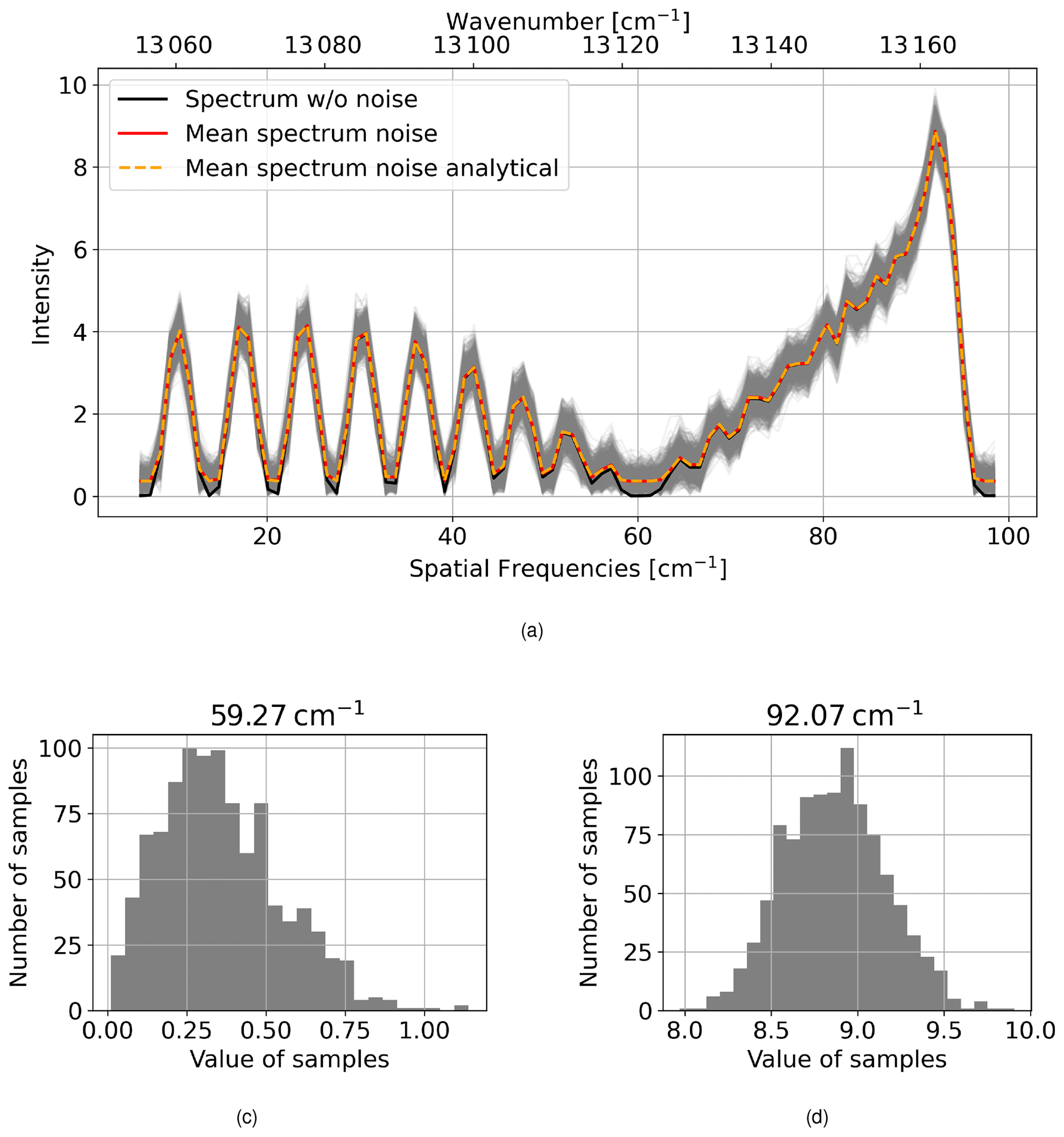
Figure A1 (a) Magnitudinal spectra for a low signal with an SNR of 20 and high temperature of 700 K with (grey lines) and without (solid black line) shot noise; the mean of the noisy spectra (red solid line) and the analytical mean calculation following the mean of the Rice distribution defined in Eq. (A5) (orange dashed line); panels (b) and (c) show the noise distribution at the minimal and maximal spectral samples at 59.27 and 92.07 cm⁻¹, respectively.

In Fig. A1a, we show magnitudinal spectra for a low signal with an SNR of 20 and high temperature of 700 K. One can see that the noisy spectra are centred around the non-noisy spectrum for high values but are off for low values. Figure A1c shows that the noise distribution is close to a normal distribution for a high value but skewed for low values as shown in Fig. A1b. Within the processing, the deviating mean is subtracted to at least centre the noise distribution around the non-noisy spectrum, which reduces the bias. Note that this affects only very low signals which are below the signal levels usually used within the processing.