Performance evaluation of three bio-optical models in aerosol and ocean color joint retrievals

Multi-angle polarimeters (MAPs) are powerful instruments to perform remote sensing of the environment. Joint retrieval algorithms of aerosols and ocean color have been developed to extract the rich information content of MAPs. These are optimization algorithms that fit the sensor measurements with forward models, which include radiative transfer simulations of the coupled atmosphere and ocean systems (CAOSs). The forward model consists of sub-models to represent the optics of the atmosphere, ocean water surface and ocean body. The representativeness of these models for observed scenes and the number of retrieval parameters are important for retrieval success. In this study, we have evaluated the impact of three different ocean bio-optical models with one, three and seven optimization parameters on the accuracy of joint retrieval algorithms of MAPs. The Multi-Angular Polarimetric Ocean coLor (MAPOL) joint retrieval algorithm was used to process data from the airborne Research Scanning Polarimeter (RSP) instrument acquired in different field campaigns. We performed ensemble retrievals along three RSP legs to evaluate the applicability of bio-optical models in geographically varying water of clear to turbid conditions. The average differences between the MAPOL aerosol optical depth (AOD) and spectral remote sensing reflectance (R_rs(λ)) retrievals and the MODerate resolution Imaging Spectroradiometer (MODIS) products were also reported. We studied the distribution of retrieval cost function values obtained for the three bio-optical models. For the one-parameter model, the spread of retrieval cost function values is narrow regardless of the type of water even if it fails to converge over coastal water. For the three- and seven-parameter models, the retrieval cost function distribution is water type dependent, showing the widest distribution over clear, open water. This suggests that caution should be used when using the spread of the cost function distribution to represent the retrieval uncertainty. We observed that the three- and seven-parameter models have similar MAP retrieval performances in all cases, though they are prone to converge at local minima over open-ocean water. It is necessary to develop a screening algorithm to divide open and coastal water before performing MAP retrievals. Given the computational efficiency and the algorithm stability requirements, we recommend the three-parameter bio-optical model as the coastal-water bio-optical model for future MAPOL studies. This study provides important practical guides on the joint retrieval algorithm development for current and future satellite missions such as NASA's Plankton, Aerosol, Cloud, ocean Ecosystem (PACE) mission and ESA's Meteorological Operational-Second Generation (MetOp-SG) mission.

1 Introduction

The enhanced capabilities in satellite remote sensing of Earth have enabled detailed observation of the atmosphere, ocean and land, thereby improving the accurate determination of spatial and temporal distributions of the constituents of each. Satellite-borne spectroradiometers in particular have substantially advanced the way we view our home planet, and their information content will increase in the future as the technology evolves from multispectral to hyperspectral capabilities. Multi-angle polarimeters (MAPs), such as the Polarization and Directionality of the Earth’s Reflectance (POLDER) (Deschamps et al., 1994), Airborne Multi-angle Spectro-Polarimetric Imager (AirMSPI) (Diner et al., 2013), Spectro-polarimeter for Planetary EXploration (SPEX) (Smit et al., 2019), Research Scanning Polarimeter (RSP) (Cairns et al., 2003), Multi-viewing Multi-Channel Multi-Polarization Imager (3MI) (Fougnie et al., 2018) and Multi-Angle Imager for Aerosols (MAIA) (Van Harten et al., 2021), have even greater information content compared to other existing single-viewing angle spectroradiometers, such as the MODerate Resolution Imaging Spectrometer (MODIS), Visible Infrared Imaging Radiometer Suite (VIIRS), and Ocean and Land Color Instrument (OLCI), owing to their ability to perform measurements at multiple viewing angles and different polarimetric states (Dubovik et al., 2019).

Atmospheric aerosols play a critical role in the Earth's climate and air quality (Boucher et al., 2013; Li et al., 2017). Aerosols affect Earth's energy balance directly by absorbing and scattering solar radiation and indirectly by interacting with clouds. Some of the traditional retrieval algorithms such as those for MODIS-like instruments result in larger aerosol and ocean color retrieval uncertainties when compared with the accuracy required for climate modeling (Remer et al., 2005; Sayer et al., 2016), which is due to the limited information content in single-viewing spectrometer measurements (Mishchenko et al., 2004). The large retrieval uncertainties of aerosols and ocean color also limit the accuracy of aerosol radiative forcing determination, thereby hindering our understanding of global climate change (Boucher et al., 2013). Improved aerosol characterization and quantification will support accurate estimation of atmospheric path radiance in the atmospheric correction (AC) process of ocean color remote sensing (Mobley et al., 2016). The spectral remote sensing reflectance (R_rs(λ) (sr⁻¹)) estimated through the AC process can be used to infer ocean optical and biogeochemical properties that are important for a broader understanding of phytoplankton dynamics, primary production, the global carbon cycle and the ocean's ecological response to climate change (Frouin et al., 2019).

AC is the process of removing atmospheric and surface contributions from the total measured signal at the top of the atmosphere (TOA) so that ocean color can be assessed. AC algorithms can be divided into two categories of processing strategies: traditional (or heritage) AC algorithms applicable to MODIS-like spectroradiometers (Gordon and Wang, 1994) and joint aerosol and ocean retrieval algorithms applicable to MAP measurements (Mishchenko and Travis, 1997; Chowdhary et al., 2001; Hasekamp and Landgraf, 2007; Knobelspiesse et al., 2012; Remer et al., 2019a, b). Traditional or heritage AC algorithms (Gordon and Wang, 1994) estimate the aerosol properties at near-infrared (NIR) wavelengths by assuming the water leaving radiance in NIR to be negligible or appropriately modeled (the so-called black pixel assumption) (Bailey et al., 2010). The aerosol properties are then extrapolated into the visible by using the appropriate aerosol models that fit NIR radiances (Zibordi et al., 2009; Gordon, 2021; Utry et al., 2014). This assumption does not unequivocally work in optically complex water, which can lead to an overestimate of aerosol path radiance either with nonzero NIR water leaving radiance or when absorbing aerosols are present (IOCCG, 2000, 2010). The heritage algorithm implemented by NASA's Ocean Biology Processing Group (OBPG; https://oceancolor.gsfc.nasa.gov, last access: 5 October 2023) works well over open water but can produce negative R_rs(λ) in blue wavelengths over turbid water (Bailey et al., 2010) given the aforementioned reasons. Efforts have been made to overcome negative R_rs(λ) (Bailey et al., 2010; He et al., 2012; Fan et al., 2021; Ibrahim et al., 2019), though the problem has not been fully resolved yet.

The second category of AC algorithms makes use of the larger information content available from MAPs. These instruments have a greater information content, which can be used to characterize aerosol microphysical properties (Mishchenko and Travis, 1997; Chowdhary et al., 2001; Hasekamp and Landgraf, 2007; Knobelspiesse et al., 2012; Remer et al., 2019a, b) and thus offer the potential for improvements in both aerosol and ocean color retrievals. Joint retrieval algorithms provide simultaneous retrievals of aerosols and ocean color by fitting the sensor measurements with forward model simulations for the coupled atmosphere and ocean system (CAOS) (Chowdhary et al., 2005; Hasekamp et al., 2011; Xu et al., 2016; Stamnes et al., 2018; Gao et al., 2018, 2019, 2020, 2021; Fan et al., 2021). The simulations are carried out by vector radiative transfer models with parameterizations that define the state of the CAOS. The difference between measurements and the model simulation is quantified by a cost function, which is minimized by iteratively perturbing the free parameters in the radiative transfer model. The forward model of ocean color joint retrieval algorithms consists of sub-models to simulate the optics of the CAOS, which is composed of the atmosphere, ocean surface and ocean body. The robustness of the joint retrieval algorithms depends on the representativeness of CAOS models over an observed scene. One important component of CAOS is the ocean bio-optical models that represent the spectral behaviors of aquatic inherent optical properties (IOP(λ)s) (e.g., pure seawater, phytoplankton, colored dissolved organic matter (CDOM) and non-algal particles (NAPs)) (IOCCG, 2006).

Ocean water is loosely classified into two categories, Cases I and II, based on the constituents present in the water and those constituents' relationships with R_rs(λ). In Case 1 water the IOP(λ)s co-vary with the presence of phytoplankton and its derived CDOM, which are typically found offshore in the open ocean. The IOP(λ)s of Case I water are typically parameterized using the concentration of the phytoplankton pigment chlorophyll a ([Chl a] [mg m⁻³]) and, hence, result in single-parameter bio-optical models. Unlike Case I water, Case II water, which is most commonly found in coastal and turbid environments, consists of phytoplankton, NAP and CDOM, none of which are ubiquitously co-varied. Consequently, multiple parameters are required to represent Case II water IOP(λ)s. Many joint retrieval algorithms (Chowdhary et al., 2005; Hasekamp et al., 2011; Xu et al., 2016; Stamnes et al., 2018) assume single-parameter bio-optical models developed for Case I water, whereas only a few algorithms (Chowdhary et al., 2012; Gao et al., 2018, 2019; Fan et al., 2021) adopt multi-parameter (three to seven parameters) bio-optical models. The choice of the bio-optical model has a great impact on the retrieval performance of joint retrieval algorithms. Fan et al. (2021) have studied the impact of different bio-optical models on retrieval accuracy, but their results were limited to radiometric measurements under a single-view angle. Gao et al. (2019) showed that a seven-parameter bio-optical model is superior in representing coastal water to the single-parameter model, though it is still an open question for the optimal bio-optical model for coastal water for joint retrieval algorithms.

The goal of this study is to examine the overall impact of bio-optical models with different numbers of free parameters on the performance and uncertainty of joint retrieval algorithms for Case II water. Hannadige et al. (2023) showed that multi-parameter bio-optical models with three and five parameters show similar retrieval performances for the semi-analytical algorithm (SAA) based on in situ multi-band R_rs(λ) measurements. An independent study showed that the number of free parameters a retrieval algorithm might meaningfully retrieve is roughly four based on in situ hyperspectral R_rs(λ) measurements (Cael et al., 2023). Here, for the first time, we have examined to which extent these conclusions hold for the joint retrieval algorithms using airborne MAP measurements, which have not been studied before. The quality of the retrievals in this study is evaluated with respect to the magnitude of the retrieval cost function values, the distribution of retrieval cost function values (Sect. 3) from the ensemble retrievals and the sanity check with MODIS retrievals. We studied the uncertainty of the different bio-optical models based on the spread of ensemble retrieval cost function values, which is important to understand the impact of the bio-optical models on the convergence behavior of the non-linear least squares fitting algorithms. This has not been examined in previous studies. Given the inherent problems associated with MODIS retrievals over optically complex scenes, we consider the MODIS products merely a reference rather than a validation dataset.

In this study the Multi-Angular Polarimetric Ocean coLor (MAPOL) joint retrieval algorithm (Gao et al., 2018, 2019, 2020) is used to evaluate the performance of the ocean bio-optical models with different numbers of free parameters. MAPOL is an optimization approach that retrieves aerosol microphysical properties (aerosol optical depth (AOD), single scattering albedo (SSA), size distribution and refractive index) and in-water properties (R_rs(λ), [Chl a] and component IOP(λ)s) simultaneously. Three bio-optical models are used, i.e., the single-parameter model for open-ocean water and two coastal bio-optical models with three and seven free parameters, respectively. The MAPOL algorithm was used to inverse the Research Scanning Polarimeter (RSP) measurements from two NASA airborne campaigns (Aerosol Characterization from Polarimeter and Lidar (ACEPOL) (https://www-air.larc.nasa.gov/missions/acepol, last access: 10 December 2022) (Knobelspiesse et al., 2020) and North Atlantic Aerosols and Marine Ecosystems Study (NAAMES) (https://www-air.larc.nasa.gov/missions/naames, last access: 10 December 2022) (Behrenfeld et al., 2019). The RSP measurements were selected such that the underlying water represents clear to turbid water conditions. The retrieval results were checked against the AOD product from MODIS and High Spectral Resolution Lidar (HSRL)-2 (Burton et al., 2013) and ocean color products (R_rs(λ) and [Chl a]) from MODIS. The retrieval uncertainties have been evaluated with respect to the Glory uncertainty requirement for AOD (Mishchenko et al., 2004) and PACE uncertainty requirements for open-ocean R_rs(λ) (Werdell et al., 2019).

The conclusions from this study can be used to provide recommendations for selecting suitable bio-optical models for joint retrieval algorithms over coastal water to improve their accuracy and computational efficiency. The larger parameter space required for Case II parameterizations leads to longer forward model simulation times or decreases in the likelihood of accurate retrieval convergence. Thus, the balance between the model fidelity and the parameter space is vital to improve retrievals and uncertainties. This study also expects one to improve the performance of the polynomial-based atmospheric correction (POLYAC) algorithm (Hannadige et al., 2021), which is an AC algorithm for hyperspectral single-view radiometers applied over optically complex scenes, such as over coastal water. POLYAC relies on collocated MAP retrievals from the MAPOL algorithm to estimate the hyperspectral path radiance to calculate hyperspectral R_rs(λ), which is crucial for retrieving phytoplankton functional types (IOCCG, 2014). Though this study was carried out with MAPOL, the conclusions are equally applicable to other joint retrieval algorithms of aerosols and ocean color, which thus have greater impacts beyond MAPOL.

This paper is organized as follows. Section 2 reviews the data used in the study; Sect. 3 describes the MAPOL algorithm and the respective bio-optical models; Sect. 4 presents the methodology and the retrieval results along with an uncertainty assessment under three different scenes; Sect. 5 discusses the overall results; and, finally, Sect. 6 summarizes the conclusions.

2 Data

2.1 Airborne data

In this study, we used airborne RSP measurements acquired from the ACEPOL 2017 (https://www-air.larc.nasa.gov/missions/acepol/index.html, last access: 10 December 2022) (Knobelspiesse et al., 2020) and NAAMES 2015 (https://www-air.larc.nasa.gov/missions/naames/index.html, last access: 10 December 2022) (Behrenfeld et al., 2019) airborne field campaigns. The ACEPOL campaign was held from 19 October to 9 November 2017, covering California, Nevada, Arizona, New Mexico and the coastal Pacific Ocean. NAAMES 2015 was the first deployment of the NAAMES campaign conducted from 5 November to 2 December 2015 over the North Atlantic Ocean.

RSP is an along-track scanner, with 152 viewing angles within ±60^∘. It has nine spectral channels spanning the visible to shortwave infrared (SWIR) with central wavelengths of each band located at 410, 470, 550, 670, 865, 960, 1590, 1880 and 2250 nm. RSP-1 and RSP-2 are two versions of the RSP instrument that differ in measurement uncertainty characterizations. RSP measurements over oceans have been used for aerosol and ocean color retrievals in multiple studies (Chowdhary et al., 2005, 2012; Stamnes et al., 2018; Gao et al., 2019, 2020) with promising performances. In the ACEPOL campaign, RSP-2 measurements were acquired with a relative radiometric characterization uncertainty of approximately 0.03 and polarimetric characterization uncertainty of about 0.002 in degree of linear polarization (DoLP), whereas in the NAAMES 2015 campaign RSP-1 measurements were acquired with radiometric (relative) and polarimetric characterization uncertainties of approximately 0.015 and 0.002, respectively. The instrument noise model for RSP is provided in Knobelspiesse et al. (2019).

We performed MAP retrievals across three RSP flight legs over selected open- and coastal-water regions. From the ACEPOL campaign, we selected a coastal leg across Monterey Bay, where the water was mostly clear offshore and turbid when closer to the coast. From the NAAMES campaign, we selected a coastal leg across Delaware Bay and an open-ocean leg offshore and outward from Delaware Bay. Each case has been named based on the campaign and the type of water present: ACEPOL-Mix, NAAMES-Coastal and NAAMES-Open. Gao et al. (2019) showed a single-pixel retrieval from the NAAMES-Coastal case inside Delaware Bay comparing the retrieval performances of one- and seven-parameter bio-optical models. The details of the three cases are summarized in Table 1 and Fig. 1. The three cases were selected based on the availability of RSP measurements in cloud-free conditions, the water turbidity of the location and the availability of desired MODIS retrieval products. The turbidity of the water was assumed based on MODIS [Chl a] retrievals (Hu et al., 2012).

Table 1 Summary of the datasets used in this study.

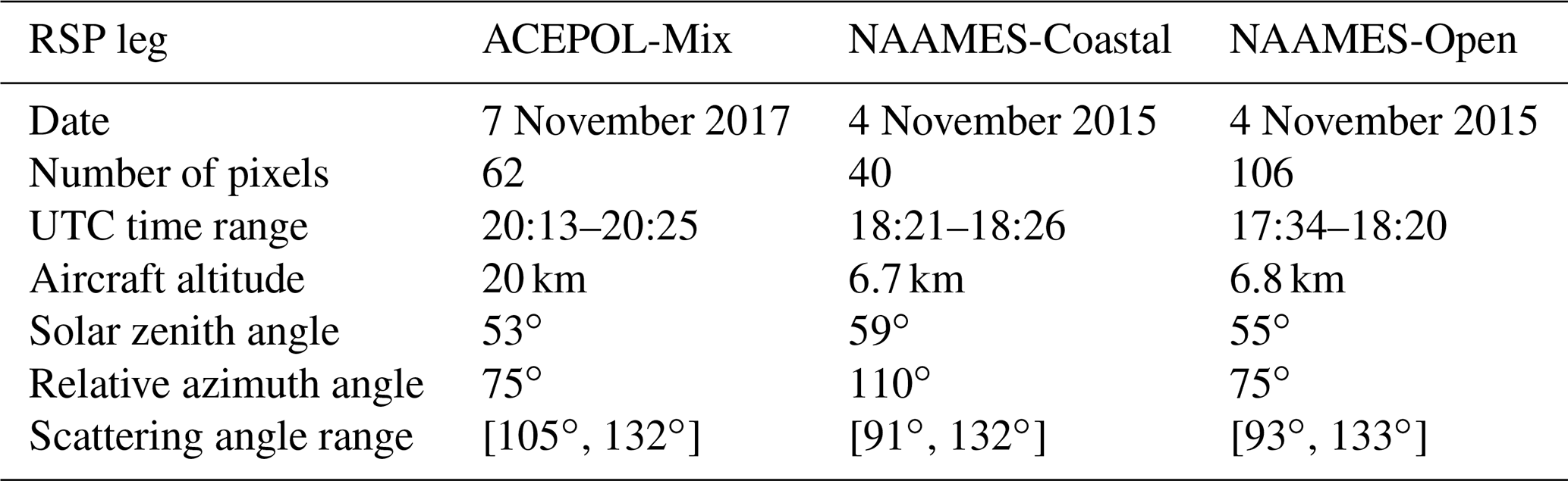
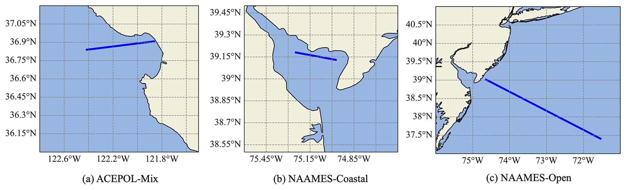
Figure 1 Geographical locations of the selected RSP legs.

RSP wavelength bands corresponding to water vapor absorption (960 and 1880 nm), as well as those wavelength bands with high noise (1590 and 2250 nm bands only for DoLP), were excluded from the retrieval. The viewing angles contaminated by Sun glint and clouds were excluded from the retrieval to reduce retrieval uncertainty. For each location of interest, five consecutive pixels along the RSP leg were averaged to achieve better measurement accuracy. The RSP legs with averaged pixels are shown in Fig. 1. For the ACEPOL and NAAMES campaigns, the size of each averaged pixel is approximately 1 and 0.5 km, respectively. The corresponding averaged measurements (reflectance and DoLP) were applied in the retrieval.

2.2 Validation data

The AOD from the ACEPOL campaign is validated against HSRL-2. Due to the lack of at-sea in situ validation data, we performed sanity checks of the retrieval results using MODIS AOD and R_rs(λ) products. MODIS is a single-view angle multispectral imager on both the NASA Terra and Aqua satellite platforms. The MODIS-OC (ocean color) product (NASA Ocean Color Web, 2020; https://oceancolor.gsfc.nasa.gov, last access: 5 October 2023) is processed using the standard NASA AC algorithm (Mobley et al., 2016) developed based on the atmospheric correction algorithm (Gordon and Wang, 1994) as modified by Ahmad et al. (2010). We used level 2 ocean color (OC) products from the MODIS instrument on board the Aqua satellite (version 2022.0). It provides a spatial coverage of 1 km resolution at nadir. The OC products include R_rs(λ) at 412, 443, 469, 488, 531, 547, 555, 645, 667 and 678 nm and [Chl a] via the Color Index-based Algorithm (CIA; Hu et al., 2012). We also obtained MODIS AOD at 869 nm and the Ångström exponent derived from the standard NASA Atmospheric Correction (AC) algorithm to estimate the spectral AOD at RSP wavelengths. The ACEPOL 2017 campaign flew the HSRL-2 along with RSP, with the former instrument also providing accurate data for AOD validation.

3 The MAPOL joint retrieval algorithm

The MAPOL joint retrieval algorithm simultaneously retrieves aerosol and ocean color properties from MAP measurements. It has been validated with synthetic RSP data (Gao et al., 2018) and real RSP (Gao et al., 2019; Hannadige et al., 2021) and SPEX airborne measurements (Gao et al., 2020; Hannadige et al., 2021).

3.1 Retrieval cost function

The algorithm minimizes the difference between the MAP measurements and forward model simulations for CAOS (Zhai et al., 2009, 2010). The forward model simulation is iteratively optimized (Levenberg–Marquardt non-linear least squares optimization) by perturbing the set of free parameters that represent the atmosphere and ocean optical properties. The least squares cost function (χ²(x)) used to quantify the difference between the measurement and the forward model simulation is defined as

$$\begin{array}{}\text{(1)}& {\mathit{\chi }}^{\mathrm{2}}\left(\mathit{x}\right)={\displaystyle \frac{\mathrm{1}}{N}}\sum _i({\displaystyle \frac{{\left[{\mathit{\rho }}_{\mathrm{t}}\left(i\right)-{\mathit{\rho }}_{\mathrm{t}}^{\mathrm{f}}(\mathit{x};i)\right]}^{\mathrm{2}}}{{\mathit{\sigma }}_{\mathrm{t}}^{\mathrm{2}}\left(i\right)}}+{\displaystyle \frac{{\left[P_{\mathrm{t}}\left(i\right)-P_{\mathrm{t}}^{\mathrm{f}}(\mathit{x};i)\right]}^{\mathrm{2}}}{{\mathit{\sigma }}_P^{\mathrm{2}}\left(i\right)}}),\end{array}$$

where ${\mathit{\rho }}_{\mathrm{t}}=\mathit{\pi }{r}^{\mathrm{2}}{L}_{\mathrm{t}}/{\mathit{\mu }}_{\mathrm{0}}{F}_{\mathrm{0}}$ is the total measured reflectance, and $P_{\mathrm{t}}=\sqrt{Q_{\mathrm{t}}^{\mathrm{2}}+U_{\mathrm{t}}^{\mathrm{2}}}/L_{\mathrm{t}}$ is the total measured DoLP. L_t, Q_t and U_t are the first three Stokes parameters measured at sensor level; μ₀ is the cosine of the solar zenith angle; F₀ is the extraterrestrial solar irradiance; and r is the Sun–Earth distance in astronomical units. ${\mathit{\rho }}_{\mathrm{t}}^{\mathrm{f}}$ and $P_{\mathrm{t}}^{\mathrm{f}}$ denote the total reflectance and DoLP simulated from the forward model. x is the state vector of the retrieval, i is the measurement index corresponding to a particular angle or wavelength, and N is the total number of measurements used in the retrieval. σ_t and σ_P are the total uncertainties of reflectance and DoLP, which include the RSP instrument characterization (Knobelspiesse et al., 2019), variance due to averaging nearby pixels and forward model uncertainties. The forward model uncertainty is estimated as 0.015 and 0.002 for the radiometric and polarimetric uncertainties, respectively (Gao et al., 2023). The uncertainty correlation between angles has been ignored (Knobelspiesse et al., 2012; Gao et al., 2023).

The χ² value of a converged retrieval indicates the goodness of fit of the retrieval. A χ² value substantially larger than 1 suggests the insufficiency of the forward model to accurately represent a given set of MAP measurements. A χ² close to 1 implies that the difference between the measurement and the corresponding forward model simulation is within the uncertainty quantified by σ_t and σ_P. In this study, we used χ² values obtained under each retrieval to assess their retrieval quality and performances.

3.2 Forward model

The forward model of the MAPOL algorithm is a vector radiative transfer model based on the successive order of scattering method (Zhai et al., 2009, 2010). The CAOS is defined as three layers: a top molecular layer, a middle layer with mixed aerosols and molecules (2 km height), and an ocean layer bounded by a rough water surface (Cox and Munk, 1954). The aerosol size distribution is composed of five spherical aerosol sub-modes: three fine modes and two coarse modes, each with a log-normal distribution. The mean radius and variance are fixed (Gao et al., 2020). The complex refractive index spectra of the two aerosol modes are based on the principal component analysis (PCA) of datasets representing spectral refractive indices of water, dust-like, biomass burning, industrial, soot, sulfate, water-soluble (Shettle and Fenn, 1979) and sea salt aerosols (de Almeida et al., 1991). The refractive indices are approximated as $m\left(\mathit{\lambda }\right)=m_{\mathrm{0}}+{\mathit{\alpha }}_{\mathrm{1}}{p}_{\mathrm{1}}\left(\mathit{\lambda }\right)$, where m₀ and α₁ are fitting parameters, and p₁(λ) is the first order of the principal component.

In the MAPOL forward model, the analytical Fournier–Forand phase function (F_p) (Fournier and Forand, 1994) is used to represent the particulate scattering phase function. The F_p is determined by B_p (i.e., $b_{\mathrm{bp}}/b_{\mathrm{p}})$ (Mobley et al., 1993). The overall phase function of water is obtained by mixing F_p with that of a pure-water phase function, which is then multiplied by the normalized Mueller matrix derived from measurements (Voss and Fry, 1984; Kokhanovsky, 2003) to obtain the total Mueller matrix of water assuming invariant polarization properties (Zhai et al., 2017).

MAPOL retrieves the spectral aerosol refractive indices described by eight parameters (two (fine and coarse) modes × two PCA × two parts (real and imaginary)); aerosol volume densities (five parameters, one for each aerosol sub-mode); one parameter to represent the roughness of ocean surface, i.e., wind (characterized by isotropic Cox Munk model; Cox and Munk, 1954); and either one, three or seven parameters to represent water IOP(λ)s depending on the choice of bio-optical model in the retrieval.

Bio-optical models

MAPOL includes two ocean bio-optical models in the forward model to represent Case I and II water separately. The Case I water bio-optical model (“C1P1”) is a single-parameter model based on [Chl a], where the number following “P” stands for the number of free parameters in the model. The Case II (“C2P7”) model contains seven bio-optical parameters. In this study, we have included a third Case II water bio-optical model with three parameters (“C2P3”). A detailed description of the bio-optical models is given below.

C2P7 (Eqs. 2–5) is a coastal or Case II bio-optical model with seven parameters.

$$\begin{array}{}\text{(2)}& {\displaystyle }{a}_{\mathrm{ph}}\left(\mathit{\lambda }\right)=A_{\mathrm{ph}}\left(\mathit{\lambda }\right)[\mathrm{Chl}a{]}^{E_{\mathrm{ph}}\left(\mathit{\lambda }\right)},\text{(3)}& {\displaystyle }{a}_{\mathrm{dg}}\left(\mathit{\lambda }\right)=a_{\mathrm{dg}}\left(\mathrm{440}\right)\exp \left[-S_{\mathrm{dg}}(\mathit{\lambda }-\mathrm{440})\right],\text{(4)}& {\displaystyle }{b}_{\mathrm{bp}}\left(\mathit{\lambda }\right)=b_{\mathrm{bp}}\left(\mathrm{660}\right){\left({\displaystyle \frac{\mathit{\lambda }}{\mathrm{660}}}\right)}^{-S_{\mathrm{bp}}},\text{(5)}& {\displaystyle }{B}_{\mathrm{p}}\left(\mathit{\lambda }\right)=B_{\mathrm{p}}\left(\mathrm{660}\right){\left({\displaystyle \frac{\mathit{\lambda }}{\mathrm{660}}}\right)}^{-S_{\mathrm{Bp}}},\end{array}$$

where a_ph(λ) (m⁻¹) is the absorption coefficient of phytoplankton parameterized in terms of [Chl a] using A_ph and E_ph spectral coefficients obtained from Bricaud et al. (1998), a_dg(λ) (m⁻¹) is the spectral absorption coefficient of CDOM and NAP, b_bp(λ) (m⁻¹) is the spectral backscattering coefficient of particulate matter, B_p(λ) is the spectral backscattering fraction of particulate matter, S_dg (nm⁻¹) is the spectral exponential slope of a_dg(λ) (in nm⁻¹), S_bp is the spectral slope of the power law function of b_bp(λ), and S_Bp is the spectral slope of the power law function of B_p(λ). The magnitudes of the spectral slopes S_dg, S_bp and S_Bp depend on the composition and the size of the oceanic particles and therefore represent microphysical properties such as refractive index, effective radius and particle size distribution slope (Jonasz, 2007). The seven free parameters are [Chl a], a_dg(440), b_bp(660), B_p(660), S_dg, S_bp and S_Bp where 440 and 660 represent reference wavelengths in nanometers (nm).

C2P3 is a three-parameter model simplified from the C2P7 model (Eqs. 2–5). To reduce the number of free parameters, we fixed the spectral slopes. S_dg typically varies between 0.01 and 0.02 nm⁻¹ in natural water. Based on the in situ measurements over oceans (Roesler et al., 1989), most of the existing bio-optical models such as the default configuration for the generalized IOP (GIOP-DC) model (Werdell et al., 2013) adopt S_dg=0.018 nm⁻¹. It has been found that the particulate backscattering ratio from in situ measurements shows little or no spectral dependence, and the mean particulate backscattering ratio is 0.010 (Chami et al., 2005; Whitmire et al., 2007). We have fixed S_Bp at 0 and assumed a spectrally invariant backscattering fraction B_p of 0.01. S_bp typically varies between 0 and 2 from small to large particles (Werdell et al., 2013). S_bp was fixed at 0.3 in this study which was obtained by a sensitivity analysis carried out by Hannadige et al. (2023). We acknowledge that these fixed values could deviate under specific water conditions. The remaining free parameters of the model are [Chl a], a_dg(440) and b_bp(660).

C1P1 (Eqs. 6–10) is a [Chl a]-based single-parameter Case I water bio-optical model (Zhai et al., 2015, 2017). The absorption coefficient of phytoplankton a_ph(λ) is the same as Eq. (2). The absorption a_dg(λ) is given by Eq. (3) as in the C2P7 model, though S_dg is fixed at 0.018 nm⁻¹, and a_dg(440) is specified by Eqs. (6) and (7) in terms of [Chl a] (IOCCG, 2006):

$$\begin{array}{}\text{(6)}& {\displaystyle }{a}_{\mathrm{dg}}\left(\mathrm{440}\right)=p_{\mathrm{2}}{a}_{\mathrm{ph}}\left(\mathrm{440}\right)\text{(7)}& {\displaystyle }{p}_{\mathrm{2}}=\mathrm{0.3}+{\displaystyle \frac{\mathrm{5.7}\times \mathrm{0.5}{a}_{\mathrm{ph}}\left(\mathrm{440}\right)}{\mathrm{0.02}+a_{\mathrm{ph}}\left(\mathrm{440}\right)}}.\end{array}$$

Similarly, b_bp(λ) is also contributed to only by phytoplankton and is expressed in terms of [Chl a] (Huot et al., 2008).

$$\begin{array}{}\text{(8)}& b_{\mathrm{bp}}\left(\mathit{\lambda }\right)=B_{\mathrm{p}}\times b_{\mathrm{p}}\left(\mathit{\lambda }\right),\end{array}$$

where b_p(λ) (m⁻¹) is the spectral scattering coefficient of particulate matter.

$$\begin{array}{}\text{(9)}& {\displaystyle }{b}_{\mathrm{p}}\left(\mathit{\lambda }\right)=b_{\mathrm{p}}\left(\mathrm{660}\right){\left({\displaystyle \frac{\mathit{\lambda }}{\mathrm{660}}}\right)}^{-S_{\mathrm{p}}}\text{(10)}& {\displaystyle }{b}_{\mathrm{p}}\left(\mathrm{660}\right)=\mathrm{0.347}[\mathrm{Chl}a{]}^{\mathrm{0.766}}\end{array}$$

In Eq. (9), S_p is the spectral coefficient of b_p. For $\mathrm{0.02}<\left[\mathrm{Chl}a\right]<\mathrm{2}$ mg m⁻³, $S_{\mathrm{p}}=-\mathrm{0.5}\left({\log }_{\mathrm{10}}\left[\mathrm{Chl}a\right]-\mathrm{0.3}\right)$. For [Chl a]>2 mg m⁻³, S_p=0. B_p is assumed to be spectrally invariant and is described as $B_{\mathrm{p}}=\mathrm{0.002}+\mathrm{0.01}(\mathrm{0.50}-\mathrm{0.25}{\log }_{\mathrm{10}}[\mathrm{Chl}a\left]\right)$. The three bio-optical models are summarized in Fig. 2.

Figure 2 The summary of the MAPOL bio-optical models. The free parameters of each model are indicated in bold.

4 Retrieval results

We performed retrievals with the MAPOL algorithm (Sect. 3) for the three cases (ACEPOL-Mix, NAAMES-Coastal and NAAMES-Open) described in Sect. 2. Separate retrievals were carried out using each bio-optical model (C2P7, C2P3 and C1P1 described in Sect. 3.3) for all the cases, regardless of the type of water they represent.

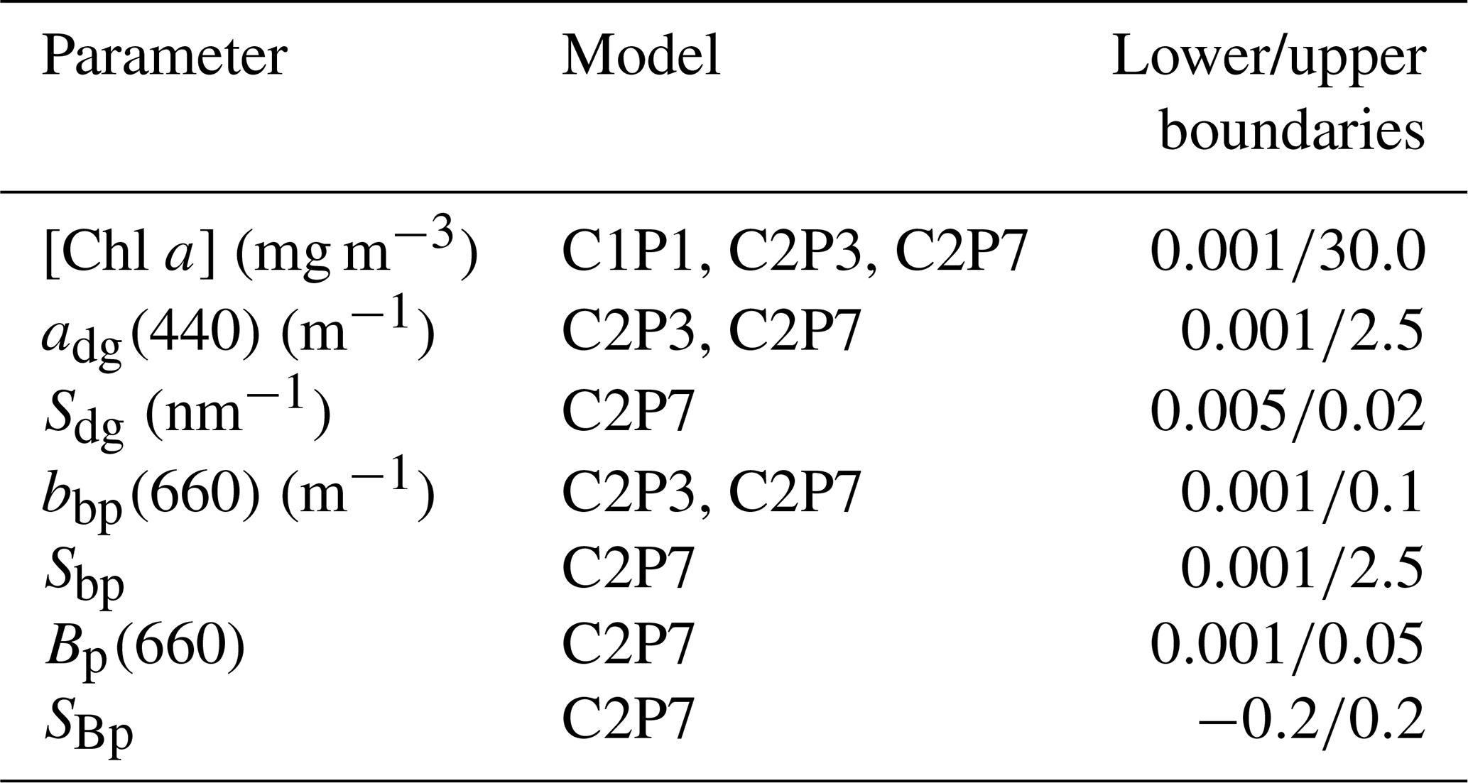
The final retrieval results are based on the ensemble retrieval technique (Gao et al., 2019, 2020). The technique can reduce the likelihood of convergence of the algorithm at local minima instead of the global minimum. The ensemble retrieval was carried out by performing 100 retrievals for each averaged RSP pixel. For each retrieval, the retrieval parameters are initialized with randomly generated initial values of each parameter, which are confined within a boundary as specified in Table 2 for bio-optical model parameters (Gao et al., 2018, 2019; Hannadige et al., 2023) and as in Gao et al. (2018) for atmospheric parameters.

Table 2 The upper and lower boundaries of the bio-optical model parameters.

The retrievals were sorted based on their χ² distribution, which is attributed to whether the ensemble of retrievals converged at the global minimum (narrow χ² distribution) or different local minima (broad χ² distribution). For each of the RSP pixels, we averaged 30 % (i.e., cumulative probability =30 %) of the total retrievals to calculate the final retrieval results. We studied average retrievals from all three bio-optical models using different cumulative probabilities at a time. About 30 % cumulative probability yielded the lowest χ² and retrieval variability. The selection of cumulative probability of less than 30 % did not leave enough ensemble retrievals to estimate the average retrieval results (for the C1P1 model this number is about 70 %; to make it consistent across all three bio-optical models, 30 % was selected). It should be noted that all the converged retrievals under the three case studies yielded χ² larger than 0.3. The minimum and maximum χ² values within this 30 % are denoted as ${\mathit{\chi }}_{min}^{\mathrm{2}}$ and ${\mathit{\chi }}_{max}^{\mathrm{2}}$, respectively. For all three cases, the selection of the first 30 % lowest χ² retrievals resulted in ${\mathit{\chi }}_{max}^{\mathrm{2}}$ values which are about five points higher than the ${\mathit{\chi }}_{min}^{\mathrm{2}}$ (that is ${\mathit{\chi }}_{max}^{\mathrm{2}}\approx \mathrm{5}+{\mathit{\chi }}_{min}^{\mathrm{2}}$). The choice of the cumulative probability or the ${\mathit{\chi }}_{max}^{\mathrm{2}}$ depends on the accuracy requirement of the retrieval.

The resultant uncertainties of the retrieval parameters are determined as the standard deviation of the retrievals within ${\mathit{\chi }}_{min}^{\mathrm{2}}$ and ${\mathit{\chi }}_{max}^{\mathrm{2}}$. The uncertainties are associated with different initial values in the optimization. Due to a large number of retrieval parameters and the non-linearity of the cost functions, the choice of the initial values often becomes important (Gao et al., 2020). Based on Gao et al. (2020) and Gao et al. (2023), the uncertainty derived from ensemble retrievals within the ${\mathit{\chi }}_{min}^{\mathrm{2}}$–${\mathit{\chi }}_{max}^{\mathrm{2}}$ range may not always be comparable to the uncertainty calculated from the error propagation method (Knobelspiesse et al., 2012). The error propagation method directly relates the retrieval uncertainties to measurement uncertainties. The evaluation of uncertainties calculated from the error propagation method is subject to future study.

4.1 ACEPOL-Mix

The minimum retrieval cost function value ${\mathit{\chi }}_{min}^{\mathrm{2}}$ is affected by the type of water present and the bio-optical model employed in the retrieval. For relatively clear water, where $\mathrm{1}<\left[\mathrm{Chl}a\right]<\mathrm{3}$ mg m⁻³, the ${\mathit{\chi }}_{min}^{\mathrm{2}}$ values obtained under all the three bio-optical models are similar ($\mathrm{2}<{\mathit{\chi }}_{min}^{\mathrm{2}}<\mathrm{3}$). The average ${\mathit{\chi }}_{min}^{\mathrm{2}}$ value within 30 % of the lowest χ² retrievals (${\mathit{\chi }}_{{\mathrm{avg}}_{\mathrm{30}\mathit{\%}}}^{\mathrm{2}}$) is comparable to the ${\mathit{\chi }}_{min}^{\mathrm{2}}$ (Fig. 3). For C2P3 and C2P7, ${\mathit{\chi }}_{{\mathrm{avg}}_{\mathrm{30}\mathit{\%}}}^{\mathrm{2}}<\mathrm{1.5}\times {\mathit{\chi }}_{min}^{\mathrm{2}}$. This suggests that the ensemble retrieval χ² values have a narrow spread attributed to the fact that most of the retrievals have reached their global minimum.

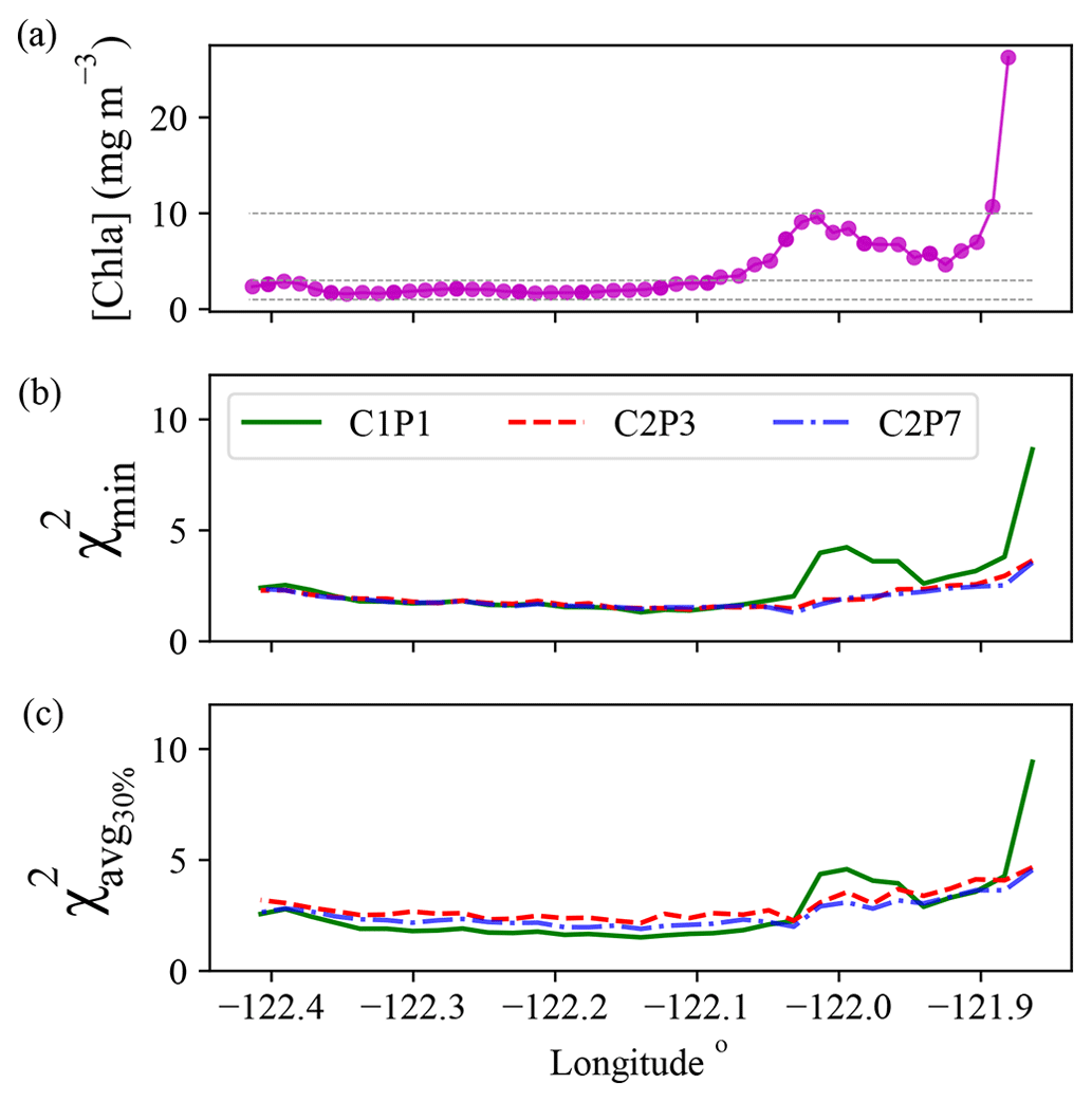
Figure 3 ACEPOL-Mix: panel (a) shows the MODIS-retrieved [Chl a]. The dashed gray lines indicate [Chl a] = 1, 3 and 10 mg m⁻³. Panel (b) shows the ${\mathit{\chi }}_{min}^{\mathrm{2}}$ obtained for the RSP retrievals across the ACEPOL-Mix leg under the three bio-optical models: C1P1, C2P3 and C2P7. Panel (c) shows the average ${\mathit{\chi }}_{min}^{\mathrm{2}}$ value for the 30 % of the lowest χ² retrievals. Data are given with respect to the longitude of the location. The coast of Monterey Bay is to the right-hand side of the plots.

With increasing turbidity towards the coast, the ${\mathit{\chi }}_{min}^{\mathrm{2}}$ values from C1P1 retrievals follow an increasing trend with increasing [Chl a]. Both the C2P3 and C2P7 models show similar ${\mathit{\chi }}_{min}^{\mathrm{2}}$ values along the track, whose ${\mathit{\chi }}_{min}^{\mathrm{2}}$ values (<5) also tend to increase with increasing [Chl a] but with less variability than that of C1P1 (${\mathit{\chi }}_{min}^{\mathrm{2}}>\mathrm{5}$). Larger ${\mathit{\chi }}_{min}^{\mathrm{2}}$ indicates the inability of the forward model to accurately fit the MAP measurement. In other words, the C1P1 model is insufficient to fully represent the turbid water IOP(λ)s compared to the C2P3 and C2P7 bio-optical models.

We further validated the retrieval results and evaluated the retrieval uncertainties (Figs. 4 and 6) associated with each bio-optical model using AOD retrievals from HSRL-2 and MODIS. MODIS and HSRL-2 AOD (Fig. 5) were collocated with RSP within a maximum distance of around 1.7 and 0.5 km. There are no in situ R_rs(λ) measurements available for validation for this scene. Instead, we compared R_rs(λ) with collocated MODIS R_rs(λ) collected within a maximum distance of 0.5 km. The time difference between MODIS and RSP measurements is roughly 1 h. The MODIS 412, 469, 555 and 667 nm ocean color bands were chosen to compare the corresponding RSP R_rs(λ) at 410, 470, 550 and 670 nm bands. AOD from RSP was compared with the MODIS AOD based on the AC data product, a choice to ensure the consistency of ocean color and aerosol data products. In this case study, the AOD and R_rs(λ) retrievals obtained by averaging 30 % of the lowest χ² cases were compared with those obtained for the ${\mathit{\chi }}_{min}^{\mathrm{2}}$ case (the results are not shown here). The comparison of RSP-retrieved AOD at 532 nm with HSRL-2 and MODIS is given in Fig. 5. For clear visualization, the density of the pixels has been reduced in the plots. The vertical bars indicate the 1σ uncertainty.

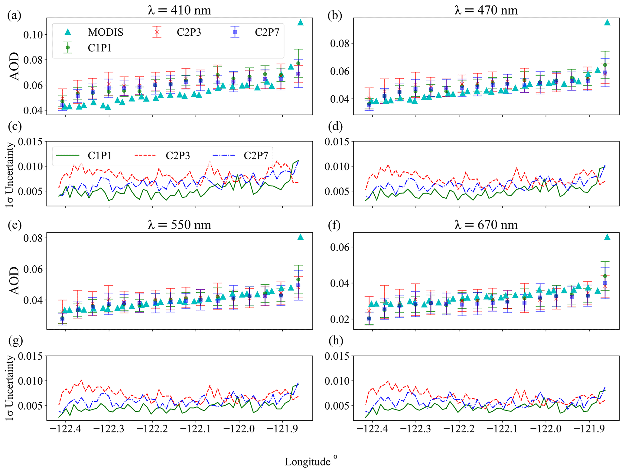
Figure 4 ACEPOL-Mix: the comparison of RSP-retrieved averaged spectral AOD across Monterey Bay with MODIS AOD and retrieval uncertainty. Results are shown for the retrievals under the three bio-optical models C1P1, C2P3 and C2P7 at 410, 470, 550 and 670 nm for averaged retrievals. The vertical bars indicate the 1σ uncertainty. Data are given with respect to the longitude of the location. The coast of Monterey Bay is to the right-hand side of the plots.

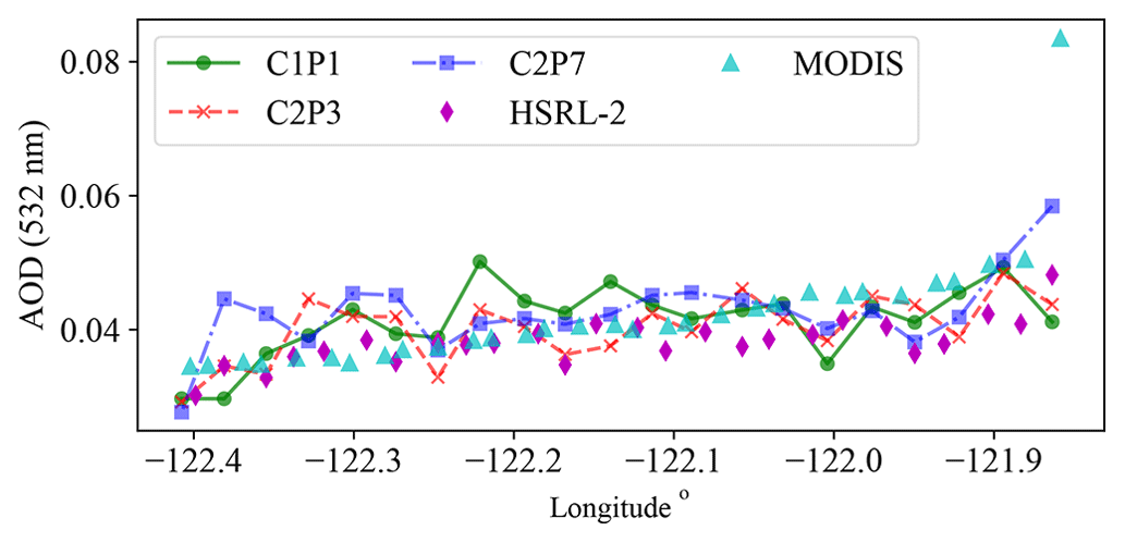
Figure 5 ACEPOL-Mix: the comparison of retrieved AOD at 532 nm with HSRL-2 and MODIS AOD at 532 nm. The AOD obtained for the lowest χ² case is shown here. Results are shown for the retrievals under the three bio-optical models C1P1, C2P3 and C2P7. Data are given with respect to the longitude of the location. The coast of Monterey Bay is to the right-hand side of the plots.

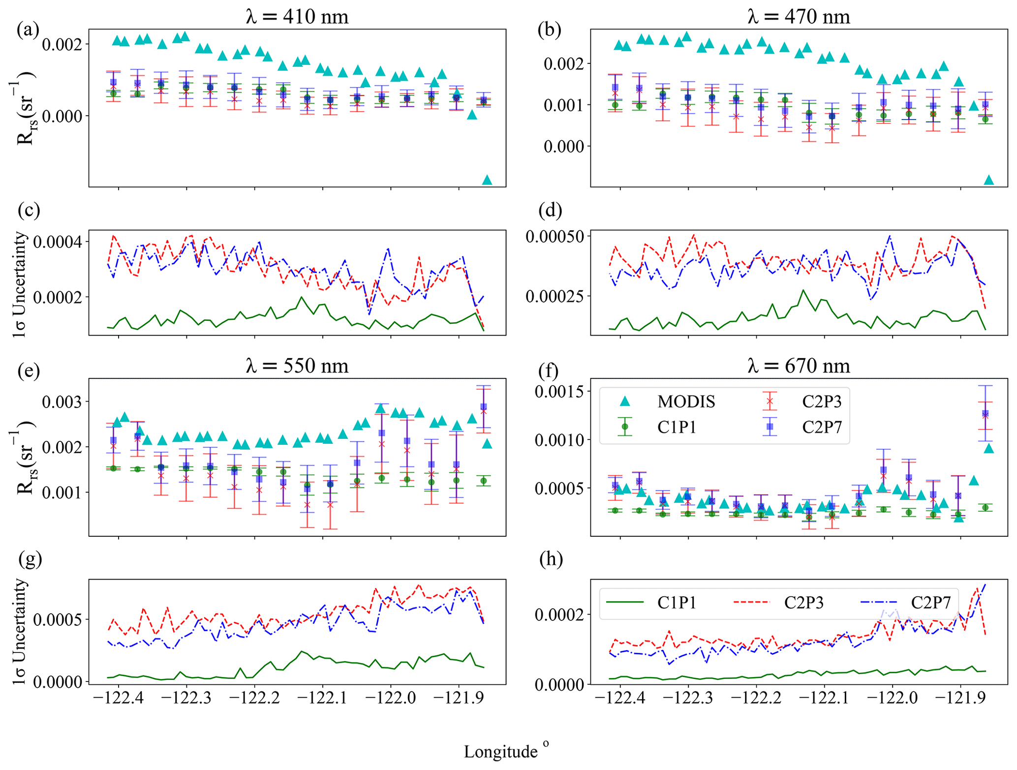
Figure 6 ACEPOL-Mix: the comparison of the RSP-retrieved averaged R_rs(λ) across Monterey Bay with MODIS R_rs(λ) product and retrieval uncertainty. Results are shown for the retrievals under the three bio-optical models C1P1, C2P3 and C2P7 at 410, 469, 554 and 670 nm for averaged retrievals. The vertical bars indicate the 1σ uncertainty. Data are given with respect to the longitude of the location. The coast of Monterey Bay is to the right-hand side of the plots.

Regardless of the selected bio-optical model or the turbidity of the water, all three models, C1P1, C2P3 and C2P7, show similar AOD values, suggesting that the bio-optical model does not substantially influence AOD retrievals (Fig. 4). Overall, the MODIS AOD agrees with the averaged MAPOL AOD within 1σ of the retrieval of all three bio-optical models, except at 410 nm, at which the MODIS AOD is slightly outside of the 1σ AOD uncertainty limits.

The AOD retrieved by HSRL-2 and MODIS at 532 nm is similar. Based on the AOD retrieval comparison with respect to HSRL-2 and MODIS at 532 nm (Fig. 5), the C2P3 model shows the overall best agreement among the three bio-optical models (Table 3). The differences between the HSRL-2, MODIS and RSP-retrieved AOD may be related to different sampling volumes, viewing geometries of the instruments and retrieval algorithms.

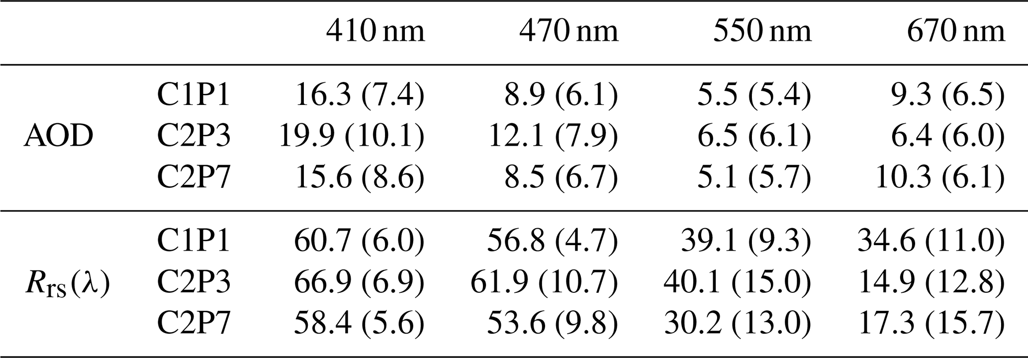
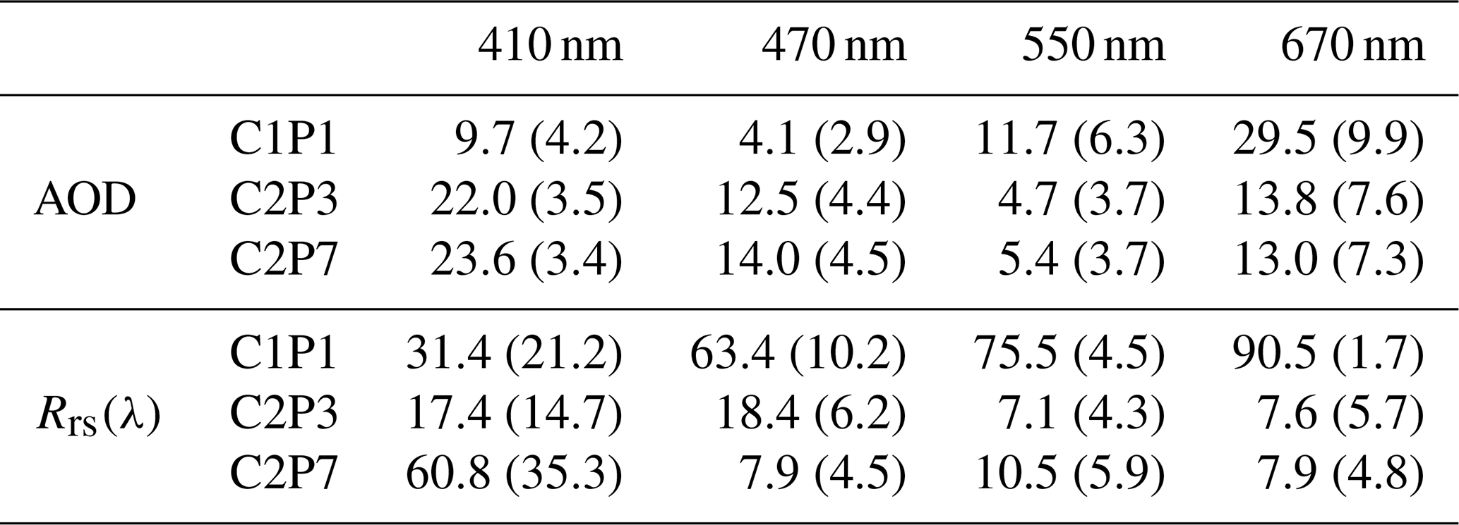
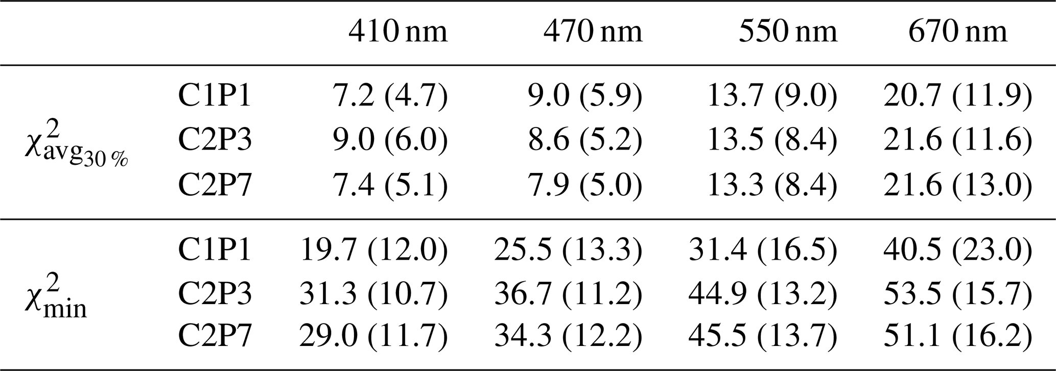
Table 3 ACEPOL-Mix: the average relative differences ($\frac{\mathrm{1}}{N}\sum \left[\frac{a_{\mathrm{model}}-a_{\mathrm{MODIS}}}{a_{\mathrm{MODIS}}}\right]\left(\mathit{\%}\right)$, where a is either AOD or R_rs(λ), and N is the total number of retrieved pixels (sample size); N=62) of AOD and R_rs(λ) between MODIS and the three bio-optical models (C1P1, C2P3 and C2P7) at 410, 470, 550 and 670 nm. Negative R_rs(λ) values from MODIS were excluded. The differences are based on 30 % averaged retrievals. The standard deviations of the relative differences are given inside the parentheses.

In the comparison of R_rs(λ) retrievals under the three bio-optical models (Fig. 6), MODIS shows negative R_rs(λ) values at shorter wavelengths (410 and 470 nm) over the one or two pixels closest to the coast around 121.95^∘ W. The AOD values over these pixels are also much larger compared to MAPOL retrievals. This indicates that the MODIS AC algorithm has overestimated the aerosol signal over coastal water, thereby making R_rs(λ) negative. There are no negative R_rs(λ) values found in the MAPOL retrievals. MODIS-estimated R_rs(λ) values are higher than those from MAPOL for relatively clear water at 410, 470 and 550 nm but agree well at 670 nm with R_rs(λ) values retrieved from the C2P3 and C2P7 models. The C1P1 model also agrees well at 670 nm but not when closer to the coast. For the MODIS, comparably larger R_rs(λ) values at shorter wavelengths can be explained by the comparably smaller AOD values at the respective wavelengths. A smaller difference in AOD can lead to a larger difference in R_rs(λ). The differences between MODIS products and MAPOL retrievals using the three bio-optical models are given in Table 3.

The corresponding retrieval uncertainties for AOD and R_rs(λ) are calculated as discussed in Sect. 4. The retrieved AOD values are similar across the three bio-optical models, but their AOD uncertainties differ due to the differences in their retrieval χ² distribution. C1P1 shows the lowest AOD and R_rs(λ) retrieval uncertainties. Yet, even though C1P1 shows smaller uncertainties compared to the other two models, the accuracy of the R_rs(λ) retrievals is not satisfactory for the two most nearshore pixels with respect to MODIS. The average uncertainty is less than 0.01 for AOD at all the given RSP wavelengths. This falls within the AOD uncertainty requirement defined by the Glory mission, namely a maximum of 0.02 over the ocean (Mishchenko et al., 2004). Overall, the C2P3 AOD uncertainty is slightly higher than that of C2P7. But it becomes smaller than that of C2P7 over the coastal water.

The R_rs(λ) uncertainty values from C2P3- and C2P7-based retrievals are similar, with a maximum of 0.0004, 0.0005, 0.0007 and 0.0003 sr⁻¹ at 410, 470, 550 and 670 nm, respectively. These uncertainties fall within the PACE-defined R_rs(λ) uncertainty: from 400 to 600 nm the absolute uncertainty is 0.0006 sr⁻¹, and from 600 to 710 nm the absolute uncertainty is 0.0002 sr⁻¹ (Werdell et al., 2019). For C1P1 the R_rs(λ) uncertainty is less than 0.0002 sr⁻¹ for all the wavelengths shown in Fig. 6 and falls within the PACE-defined R_rs(λ) uncertainty.

The C1P1 AOD uncertainty is comparable with the other two models, but C1P1 R_rs(λ) uncertainty is significantly lower than the other two models. One reason can be explained as the total number of free parameters in the retrieval. With the C1P1 model, there are a total of 15 parameters to be retrieved. For C2P3 and C2P7, that increases to 17 and 21, respectively. With fewer parameters, it is easier to converge at the global minimum within the parameter space, or a similar local minimum is always achieved. Here, for the C1P1 model, the majority of the retrievals are converged to the same point (either a local minimum or the global minimum); hence, the uncertainty defined by the spread of the cost function values is relatively small. With a larger number of free parameters in the retrieval, convergence can be achieved at a local minimum more often than at the global minimum. That makes the χ² distribution widespread; hence, the uncertainty becomes larger. Since C2P3 is a simplified version of the C2P7 model (that is a subset of the C2P7 model), we can expect C2P3 and C2P7 to have similar performances.

4.2 NAAMES-Coastal

The NAAMES-Coastal case (4 November 2015) covers RSP retrievals over Delaware Bay (Fig. 1b), which is a coastal-water region with high turbidity. The ${\mathit{\chi }}_{min}^{\mathrm{2}}$ value obtained for each pixel with the three bio-optical models (C1P1, C2P7 and C2P3) is given at the bottom of Fig. 7. The averaged ${\mathit{\chi }}_{min}^{\mathrm{2}}$ for the 30 % of the lowest χ² (${\mathit{\chi }}_{{\mathrm{avg}}_{\mathrm{30}\mathit{\%}}}^{\mathrm{2}}$) cases is the same as ${\mathit{\chi }}_{min}^{\mathrm{2}}$ for C1P1 and roughly twice the ${\mathit{\chi }}_{min}^{\mathrm{2}}$ value for both C2P3 and C2P7. We did not see a significant difference between the retrieval results obtained from the lowest χ² case and 30 % average; hence, only the averaged AOD and R_rs(λ) retrievals are shown here. The MODIS [Chl a] data (Fig. 7) show values larger than 5 mg m⁻³, and the peak value exceeds 20 mg m⁻³. The C1P1 model has shown the highest ${\mathit{\chi }}_{min}^{\mathrm{2}}$ values around 100 still with a narrow χ² distribution, whereas both C2P3 and C2P7 models show ${\mathit{\chi }}_{min}^{\mathrm{2}}$ values around 1.5. The large ${\mathit{\chi }}_{min}^{\mathrm{2}}$ values around 100 with narrow χ² distributions imply the insufficiency of the C1P1 model to represent highly turbid coastal water. This also suggests that caution needs to be taken when using the cost function spread to study the uncertainty of retrieval parameters. Overall, the C2P3 and C2P7 models show the same capability to represent turbid coastal water.

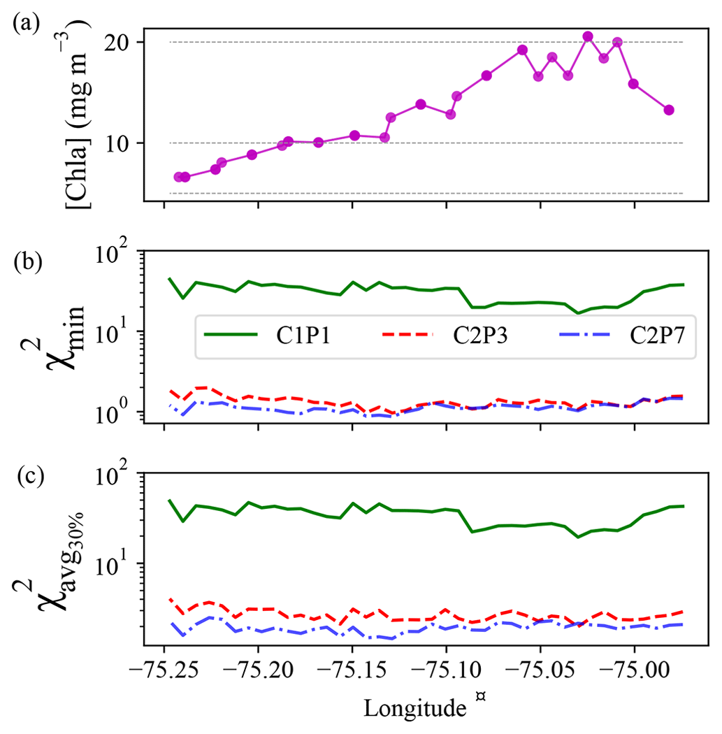
Figure 7 NAAMES-Coastal: panel (a) shows MODIS [Chl a]. The dashed gray lines indicate [Chl a] = 5, 10 and 20 mg m⁻³. Panel (b) shows ${\mathit{\chi }}_{min}^{\mathrm{2}}$ obtained for the RSP retrievals under the three bio-optical models: C1P1, C2P3 and C2P7. Panel (c) shows the average ${\mathit{\chi }}_{min}^{\mathrm{2}}$ value for the 30 % of the lowest χ² retrievals. Data are given with respect to the longitude of the location. The RSP leg is located along the eastward coast of Delaware Bay.

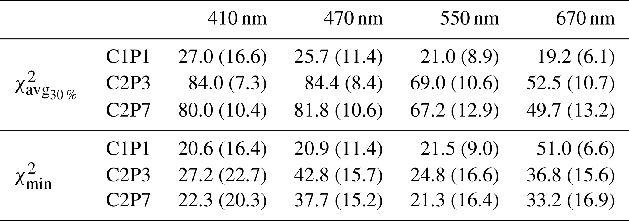
The averaged AOD obtained under the C1P1 model is larger than that obtained with C2P3 and C2P7, likely because the C1P1 model misrepresents the water properly in Delaware Bay (Fig. 8). We collocated the MODIS AOD and ocean color products within a maximum distance of 0.8 km. The time difference between MODIS and RSP scanning times is approximately 1 h. The MODIS AOD values at 410 nm are within the uncertain limits of C1P1 and fall within the uncertainty limits of C2P3 and C2P7 at the rest of the wavelengths. Correspondingly, the C1P1 R_rs(λ) is less than that from C2P3 and C2P7 (Fig. 9). At 410 and 470 nm, the R_rs(λ) retrieved with C2P7 is on average larger than that from C2P3, but similar values are retrieved at 550 and 670 nm. The MODIS R_rs(λ) agrees well with C2P3 and C2P7 at 470, 550 and 670 nm. At 410 nm, MODIS R_rs(λ) is mostly similar to that retrieved from C2P3. The average relative differences between MODIS AOD and R_rs(λ) with MAPOL retrievals under the three bio-optical models are given in Table 4.

Figure 8 NAAMES-Coastal: the comparison of the RSP-retrieved averaged AOD across Delaware Bay with MODIS AOD and uncertainty. Results are shown for the retrievals under the three bio-optical models C1P1, C2P3 and C2P7 at 410, 470, 550 and 670 nm for averaged retrievals. The vertical bars indicate the 1σ uncertainty. Data are given with respect to the longitude of the location. The RSP leg is located along the eastward coast of Delaware Bay.

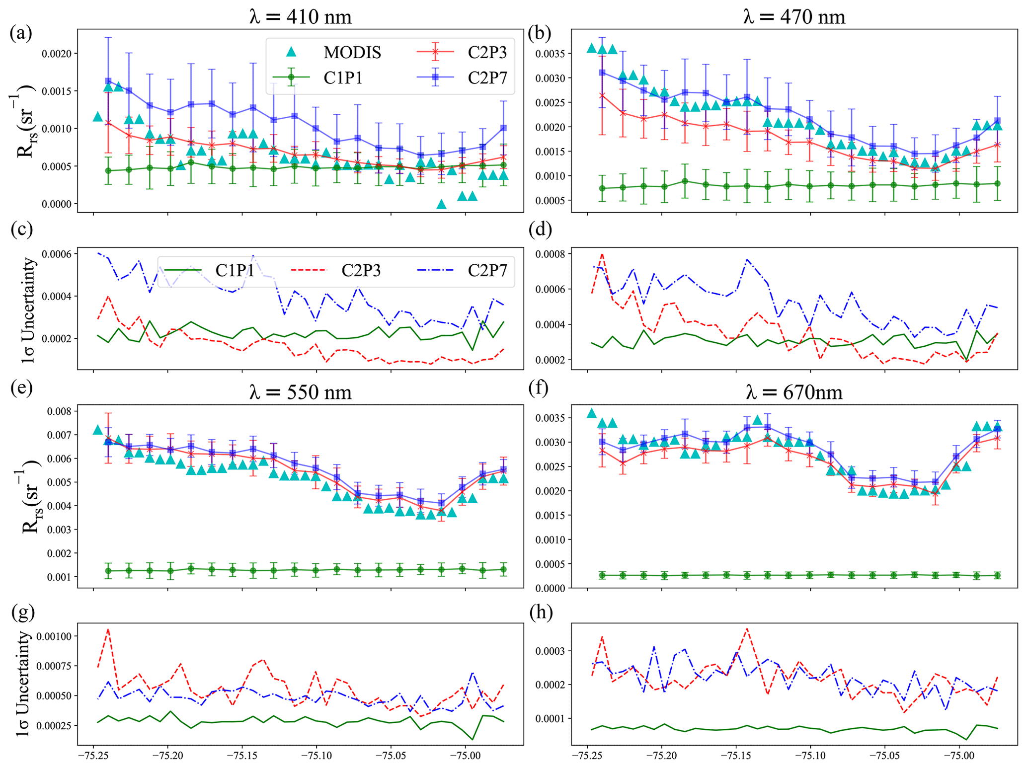
Figure 9 NAAMES-Coastal: the comparison of the RSP-retrieved averaged R_rs(λ) across Delaware Bay with MODIS R_rs(λ) product and uncertainty. Results are shown for the retrievals under the three bio-optical models C1P1, C2P3 and C2P7 at 410, 470, 550 and 670 nm for averaged retrievals. The vertical bars indicate the 1σ uncertainty. Data are given with respect to the longitude of the location. The RSP leg is located along the eastward coast of Delaware Bay.

Table 4 NAAMES-Coastal: the average relative differences (%) of AOD and R_rs(λ) between MODIS and the three bio-optical models (C1P1, C2P3 and C2P7) at 410, 470, 550 and 670 nm. Sample size is N=40. The differences are based on 30 % averaged retrievals. Negative R_rs(λ) values from MODIS were excluded. The standard deviations of the relative differences are given inside the parentheses.

The AOD and R_rs(λ) retrieval uncertainties (Figs. 8 and 9) are generally similar across the three bio-optical models, with a few exceptions seen for C1P1 R_rs(λ) uncertainty at longer wavelengths. The average AOD uncertainty is less than 0.02 at all the given RSP wavelengths and meets the AOD uncertainty requirement for climate models as assessed by Mishchenko et al. (2004). The R_rs(λ) uncertainty for the C2P7 model is larger at shorter wavelengths (410 and 470 nm), where the corresponding R_rs(λ) signals are small. Overall, the C2P3 and C2P7 models result in R_rs(λ) uncertainties near the uncertainty defined by the PACE mission except at 670 nm. Even though the R_rs(λ) retrieval uncertainties are very small, the significantly larger χ² values under the C1P1 model and the inability to match the MODIS retrievals suggest that the C1P1 model is not suitable to represent the coastal-water properties.

4.3 NAAMES-Open

The NAAMES-Open case (4 November 2015) covers RSP retrievals along the open ocean outward from Delaware Bay (Fig. 1c). The ${\mathit{\chi }}_{min}^{\mathrm{2}}$ values obtained for each pixel, under the three bio-optical models (C1P1, C2P7 and C2P3), are shown in Fig. 10b. The averaged ${\mathit{\chi }}_{min}^{\mathrm{2}}$ for the 30 % of the lowest χ² cases is the same as ${\mathit{\chi }}_{min}^{\mathrm{2}}$ for C1P1, and around 5 times the ${\mathit{\chi }}_{min}^{\mathrm{2}}$ value for both C2P3 and C2P7, showing larger χ² distributions. This implies that the C2P3 and C2P7 models result in retrievals that converge at different local minima, instead of the global minimum. The MODIS [Chl a] values (Fig. 10a) are less than 0.5 mg m⁻³ in the open ocean and increase up to 4 mg m⁻³ closer to the coast/Delaware Bay. The ${\mathit{\chi }}_{min}^{\mathrm{2}}$ values are similar across all three bio-optical models with values around 1. There are some pixels from longitude 71.5 to 72.3^∘ W which show larger ${\mathit{\chi }}_{min}^{\mathrm{2}}$ values, which we found to be attributed to cirrus cloud contamination.

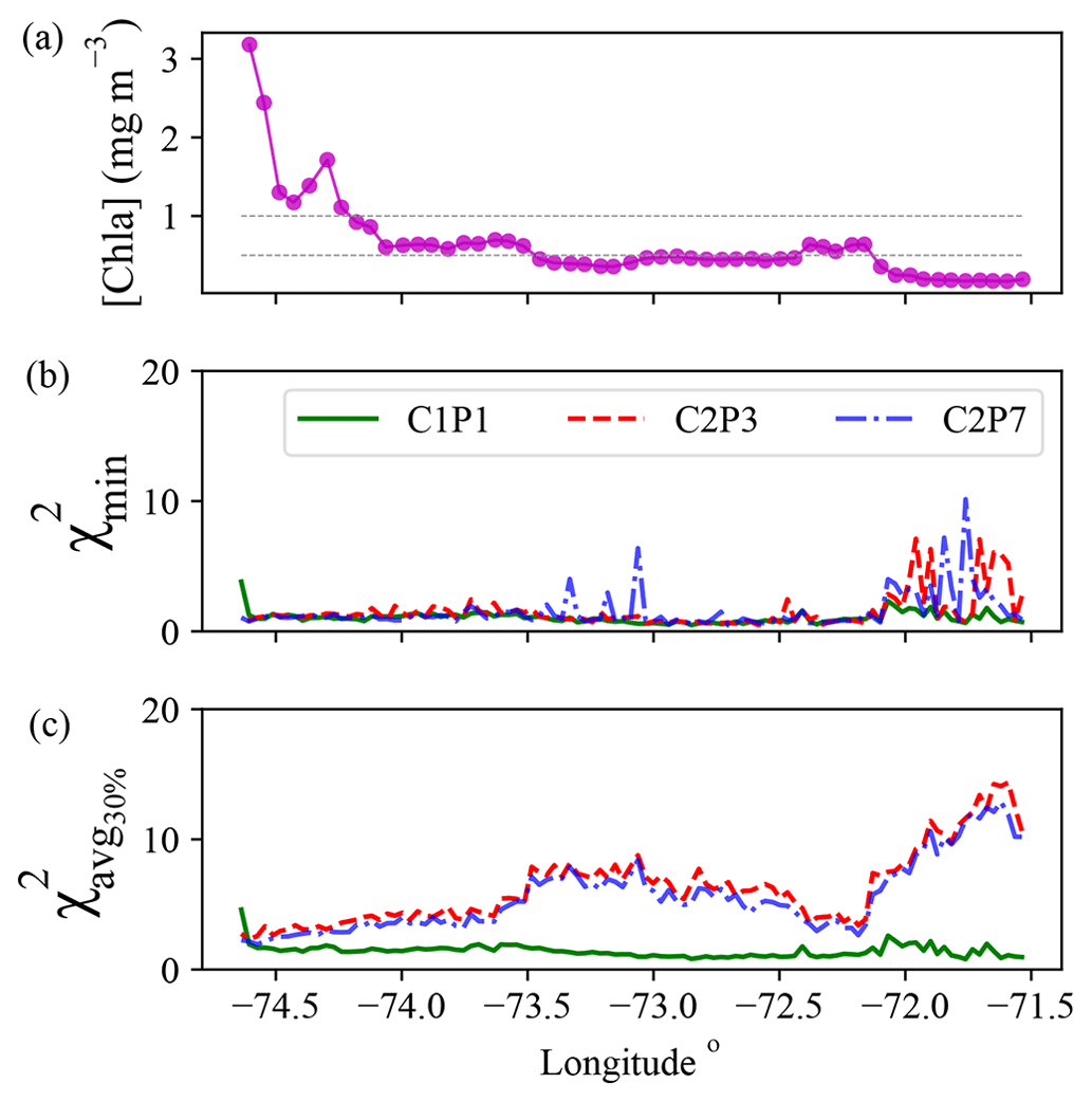
Figure 10 NAAMES-Open: panel (a) shows MODIS [Chl a]. The dashed gray lines indicate [Chl a] =0.5 and 1 mg m⁻³. Panel (b) shows ${\mathit{\chi }}_{min}^{\mathrm{2}}$ obtained for the RSP retrievals under the three bio-optical models: C1P1, C2P3 and C2P7. Panel (c) shows the average ${\mathit{\chi }}_{min}^{\mathrm{2}}$ value for the 30 % of the lowest χ² retrievals. Data are given with respect to the longitude of the location. The coast is to the left-hand side of the plots.

For this case, we collocated MODIS AOD and R_rs(λ) within a maximum distance of 1.4 and 0.5 km, respectively. The time difference between MODIS and RSP scanning times is 1 h. The comparison with MODIS AOD (Fig. 11) shows a better agreement with averaged AOD retrievals from all three bio-optical models. Some exceptions are seen in the locations that were attributed to cloud contamination. Unlike the previous two cases, the C1P1-averaged R_rs(λ) values show the best agreement with MODIS R_rs(λ) values, mostly over open water (Fig. 12). The C2P3- and C2P7-averaged R_rs(λ) values show better agreement only when closer to the coast (−74.5^∘ W), where C1P1 is not expected to provide a complete representation of the water optical properties.

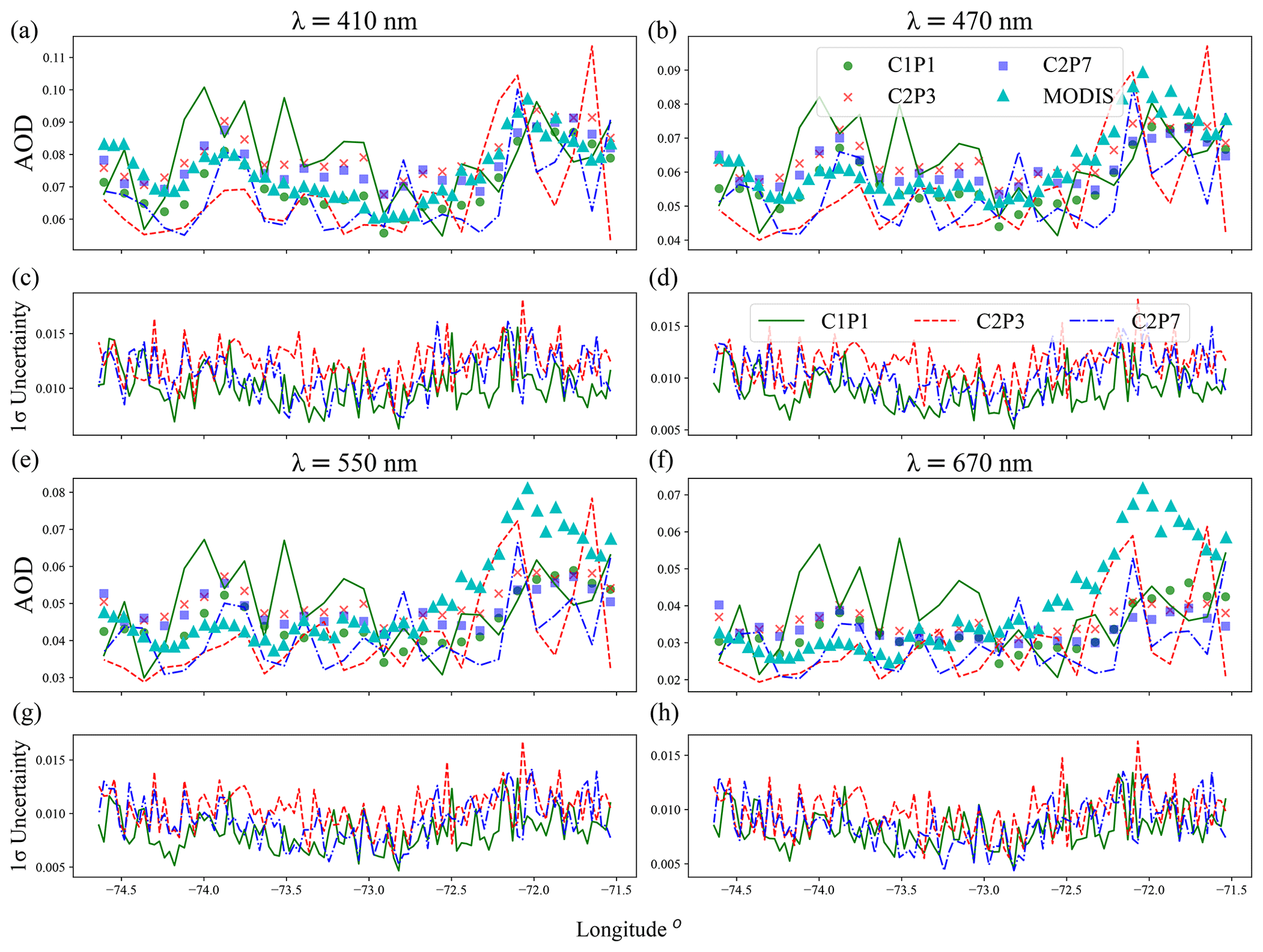
Figure 11 NAAMES-Open: the comparison of the RSP-retrieved spectral AOD across the open ocean with MODIS AOD and uncertainty. Results are shown for the retrievals under the three bio-optical models C1P1, C2P3 and C2P7 at 410, 469, 554 and 670 nm for averaged retrievals. The lines (C1P1 – solid, C2P3 – dashed, C2P7 – dotted) indicate the retrievals obtained for the ${\mathit{\chi }}_{min}^{\mathrm{2}}$ case. The markers show the average retrieval. The uncertainty plots show the 1σ uncertainty for averaged retrievals. Data are given with respect to the longitude of the location. The coast is to the left-hand side of the plots.

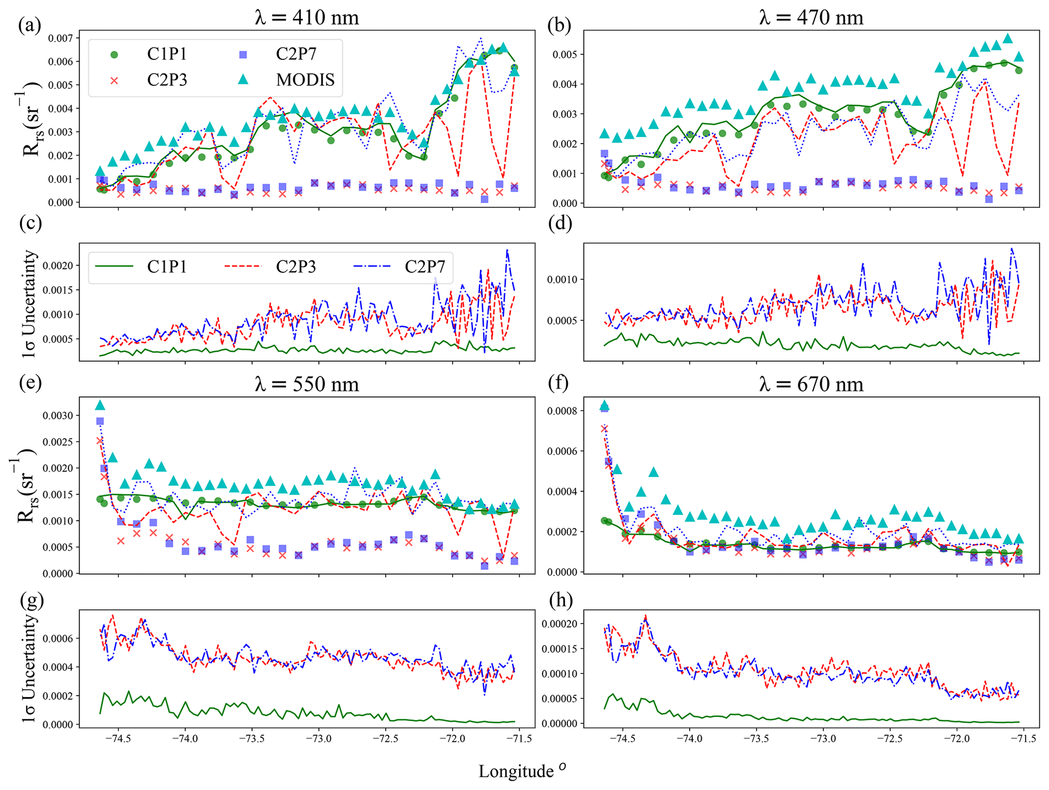
Figure 12 NAAMES-Open: the comparison of the RSP-retrieved spectral R_rs(λ) across the open ocean with MODIS R_rs(λ) product and uncertainty. Results are shown for the retrievals under the three bio-optical models C1P1, C2P3 and C2P7 at 410, 469, 554 and 670 nm for averaged retrievals. The lines (C1P1 – solid, C2P3 – dashed, C2P7 – dotted) indicate the retrievals obtained for the ${\mathit{\chi }}_{min}^{\mathrm{2}}$ case. The markers show the average retrieval. The uncertainty plots show the 1σ uncertainty for averaged retrievals. Data are given with respect to the longitude of the location. The coast is to the left-hand side of the plots.

For the C2P3 and C2P7 models, the comparison of R_rs(λ) retrievals obtained for the lowest χ² retrieval of the ensemble retrieval shows better agreement with MODIS R_rs(λ) compared to the averaged retrievals. For AOD, the C2P3- and C2P7-averaged retrievals show a better agreement with MODIS AOD than the lowest χ² retrievals. However, the agreement of the lowest χ² AOD retrievals from C2P3 and C2P7 with MODIS is better than that from C1P1. The relative differences between MODIS- and MAPOL-retrieved AOD corresponding to ${\mathit{\chi }}_{min}^{\mathrm{2}}$ and ${\mathit{\chi }}^{{\mathrm{avg}}_{\mathrm{30}\mathit{\%}}}$ are given in Table 5, and the same for R_rs(λ) is given in Table 6. There is a significant difference seen in the relative difference values between ${\mathit{\chi }}_{min}^{\mathrm{2}}$ and ${\mathit{\chi }}_{{\mathrm{avg}}_{\mathrm{30}\mathit{\%}}}$ for R_rs(λ) which is not significant for AOD. The distribution of χ² values in the ensemble retrieval therefore largely affects the accuracy of R_rs(λ) retrievals.

Table 5 NAAMES-Open: the average relative differences (%) of AOD between MODIS and the three bio-optical models (C1P1, C2P3 and C2P7) at 470, 550 and 670 nm. Sample size is N=106. The differences are given for the retrievals from ${\mathit{\chi }}_{min}^{\mathrm{2}}$ case and averaged retrievals ${\mathit{\chi }}_{{\mathrm{avg}}_{\mathrm{30}\mathit{\%}}}^{\mathrm{2}}$. The standard deviation of the relative differences is given inside the parentheses.

Table 6 The same as Table 5 but for R_rs(λ).

The AOD uncertainties (Fig. 11) are similar across the three bio-optical models, with a maximum of 0.015 at all given wavelengths. For R_rs(λ) (Fig. 12) C1P1 shows the lowest uncertainties owing to its small parameter space, which leads to better convergence near the global minimum. The multi-parameter models show comparably larger R_rs(λ) uncertainties that are still within the PACE-defined uncertainties except at 410 nm.

5 Discussion

In this study, we have evaluated the retrieval performances of three bio-optical models within CAOSs under different water conditions. For the ACEPOL-Mix case, the water varies from relatively clear to highly turbid conditions, with [Chl a] values ranging from 1–20 mg m⁻³. The NAAMES-Coastal case includes RSP measurements over highly turbid water ($\mathrm{5}<\left[\mathrm{Chl}a\right]<\mathrm{20}$ mg m⁻³). For the NAAMES-Open case, the water is mostly clear and becomes turbid when closer to the coast ($\mathrm{0.1}<\left[\mathrm{Chl}a\right]<\mathrm{3}$ mg m⁻³).

We have evaluated the retrieval performances based on the magnitude of the retrieval cost function values, the spread of the cost function distribution, the validity of the retrieved AOD and R_rs(λ) values, and the corresponding retrieval uncertainties. For the NAAMES-Open case, the C1P1 model shows low ${\mathit{\chi }}_{min}^{\mathrm{2}}$ values, indicating good fitting against RSP measurements. The C2P3 and C2P7 models also show good fitting with the RSP measurements but only when the ${\mathit{\chi }}_{min}^{\mathrm{2}}$ cases are considered. The C1P1 model shows the best agreement in AOD and R_rs(λ) retrieval results with independent data sources from the MODIS. The C1P1 retrieval performance in the ACEPOL-Mix case is satisfactory when the water is relatively clear ([Chl a]<3 mg m⁻³), that is, towards the open ocean. The C2P3 and C2P7 models in the NAAMES-Coastal case and nearshore ACEPOL-Mix pixels show better agreement in averaged AOD and R_rs(λ) retrievals with uncertainties within the Glory uncertainty requirement for AOD and the PACE uncertainty requirement for R_rs(λ).

The overall results indicate that the choice of bio-optical model (either a single parameter or multi-parameter) affects the accuracy of the retrievals, which is especially true for R_rs(λ) retrievals. Hannadige et al. (2023) showed similar retrieval performances for three- and five-parameter bio-optical models when R_rs(λ) is inverted using SAA-based algorithms. Here we demonstrated that the joint retrieval performances of the C2P3 and C2P7 models are mostly similar, showing that the same conclusion holds for joint retrieval algorithms using the airborne MAP measurements. For coastal water, it is inappropriate to use the single-parameter bio-optical model. The C2P3 and C2P7 models show good retrieval performances over turbid water.

We have also evaluated the distribution of ensemble χ² values based on ${\mathit{\chi }}_{min}^{\mathrm{2}}$ and ${\mathit{\chi }}_{{\mathrm{avg}}_{\mathrm{30}\mathit{\%}}}^{\mathrm{2}}$ values. The study of cost function distributions helps us understand the impact of bio-optical models on the convergence behavior of the non-linear least squares fitting algorithms. For the C1P1 model, the χ² distribution from all three cases is narrow, and even the resultant χ² values are large. This suggests that the use of cost function distribution alone to study the uncertainty of retrieval parameters is misleading. For C2P3 and C2P7, over moderately to highly turbid water (ACEPOL-Mix and NAAMES-Coastal, $\mathrm{1}<\left[\mathrm{Chl}a\right]<\mathrm{20}$ mg m⁻³), the χ² values are mostly closer to 1, and the distribution is nearly narrow, implying their capability to reach near the global minimum with multiple parameters over coastal water. But in the NAAMES-Open case, C2P3 and C2P7 show widespread χ² distributions, implying their inability to reach the global minimum with multiple parameters over open water. This can be explained by the degrees of freedom in the water leaving signal and the number of optimization parameters in the bio-optical models.

In the NAAMES-Open case, even though the averaged retrieval results from C2P3 and C2P7 are on average not satisfactory over clear water, the retrieval results corresponding to the lowest χ² show good agreement with MODIS AOD and R_rs(λ). This implies that the C2P3 and C2P7 models can accurately represent clear water optical properties with proper interpretation and conscientious use of the χ² distributions. However, the averaged retrieval results differ significantly, as the retrieval χ² distributions under the C2P3 and C2P7 models are widespread compared to that of C1P1. For the practical use of these bio-optical models, we suggest performing initial retrievals using the C1P1 bio-optical model and then re-performing the retrievals with either C2P3 or C2P7 models in case the C1P1 model results in significantly larger χ² values.

The C2P3 and C2P7 models show similar retrieval performances for all three case studies. The MAPOL retrievals under the C2P3 model use 17 retrieval parameters, whereas the C2P7 model uses 21 parameters. The C2P7 provides a larger parameter space that encompasses all the possible parameter value combinations of the C2P3 model; hence, their performances are similar. MAPOL is computationally demanding, as it needs to iteratively run the radiative transfer forward model for CAOS. The algorithm stability and the time taken for a single retrieval are proportional to the size of the retrieval parameters. For the C2P3 model, it takes an average of 3 h for a single CPU core to process one-pixel retrieval with RSP measurements, whereas for the C2P7 model the time increases up to 8 h, since an increased number of parameters leads to more forward model and Jacobian evaluations in least squares fitting algorithms. Therefore, the C2P3 model is more efficient for the MAPOL algorithm to represent Case II water.

The operational version of MAPOL, called FastMAPOL, replaces the radiative transfer forward model with neural networks, which can process several pixels within a second in a single CPU (Gao et al., 2021). We expect to update both the MAPOL and FastMAPOL algorithms with the C2P3 model in the future. The fixed parameters in the three-parameter C2P3 model might not be true for all the water, which is subject to fine-tuning. The availability of airborne MAP measurements over the oceans under cloud-free conditions is limited, and we cannot cover a larger range of atmosphere and water conditions in this study. The unavailability of accurate in situ measurements over the selected locations for the validation is yet another limitation. We expect to further improve our bio-optical models based on the MAP measurements to be acquired from the PACE mission plan to launch in early 2024.

The [Chl a] alone does not fully represent the turbidity of the water, as the sediment/NAP concentration and CDOM availability are also important factors. There is no clear boundary between Case I and II water (IOCCG, 2000); hence, we cannot provide a clear set of conditions where we need to apply each of the bio-optical models used in this study. There is no universal bio-optical model to represent water bio-optical properties (Fan et al., 2021). At least two separate bio-optical models are required to represent Case I and II water. The three cases in this study do not cover inland/lake water. The applicability of C2P3 and C2P7 to lakes or inland water is subject to a future study.

6 Conclusions

In this paper, we have evaluated the performance of the MAPOL joint retrieval algorithm using three bio-optical models. The RSP measurements from different field campaigns covering different water types are used. The retrieval performance evaluation is based on the magnitude of the cost function values (χ²), the spread of the retrieval cost function distribution, the validity of retrieved AOD, and R_rs(λ) values and their respective uncertainty analysis. The three bio-optical models include C1P1, a single-parameter Case I water model, and C2P3 and C2P7, which are multi-parameter Case II bio-optical models. Three cases, ACEPOL-Mix, NAAMES-Costa and NAAMES-Open, were selected based on their location and water turbidity observed with respect to [Chl a] derived from the NASA OBPG algorithm with MODIS measurements. NAAMES-Coastal covers highly turbid water, ACEPOL-Mix covers highly turbid and relatively clear water, and NAAMES-Open covers open clear water. The retrieved AOD was validated against that from HSRL-2 (ACEPOL-Coastal) and/or MODIS, and R_rs(λ) was compared against that from MODIS. The MODIS R_rs(λ) over highly turbid water shows negative values for shorter wavelengths (410 and 470 nm) that, hence, cannot be used as a validation dataset. On the other hand, the MODIS data products are used to perform sanity checks of the RSP-based MAPOL retrievals.

We evaluated the spread of the retrieval cost function distribution from the ensemble retrievals with the three bio-optical models. The C1P1 model showed narrow χ² distributions regardless of the type of water present or the magnitude of ${\mathit{\chi }}_{min}^{\mathrm{2}}$ values. This makes the retrieval uncertainty from the C1P1 model smaller, even though the model cannot accurately represent a particular water type (large cost function values). Therefore convergence has to be ensured before the uncertainty evaluation, since the use of cost function distribution alone to study the retrieval uncertainties can be misleading. The C2P3 and C2P7 models showed the widest cost function distributions over open water, with ${\mathit{\chi }}_{min}^{\mathrm{2}}$ comparable to that of C1P1. C2P3 and C2P7 showed narrow χ² distributions over moderately to highly turbid water with small χ² values. These observations implied the ability of the retrievals based on multi-parameter bio-optical models to converge near the global minimum over different water.

We also observed that the retrieval accuracies of AOD and R_rs(λ) are directly related to the choice of the bio-optical model (single parameter or multi-parameter) in the retrieval. The R_rs(λ) retrieval is significantly affected. The C1P1 model shows good retrieval performances only over relatively clear water ([Chl a]<3 mg m⁻³). The results suggested that the multi-parameter models C2P3 and C2P7 are better at representing turbid coastal water. The C2P3 and C2P7 models also have the potential to accurately represent clear open water (NAAMES-Open) in joint retrieval algorithms but with a conscientious interpretation of their χ² distributions. The C2P3 and C2P7 models tend to converge to local minima, and the extensive spread of χ² values diminishes the ability of multi-parameter models to retrieve clear water accurately and makes the interpretation of the retrieval results difficult. Therefore, it is preferred to develop screening algorithms to divide open and coastal water before performing MAP retrievals.

Similar to the SAA-based R_rs(λ) inversions (Hannadige et al., 2023), multi-parameter models (C2P3 and C2P7) perform equally well when used with joint retrieval algorithms and airborne MAP measurements. The C2P3 model is more computationally efficient than the C2P7 model, as fewer free parameters lead to significantly less processing time and more stable retrieval performances.