Raman lidar-derived optical and microphysical properties of ice crystals within thin Arctic clouds during PARCS campaign

Cloud observations in the Arctic are still rare, which requires innovative observation techniques to assess ice crystal properties. We present an original approach using the Raman lidar measurements applied to a case study in northern Scandinavia. The vertical profiles of the optical properties, the effective radius of ice crystals and ice water content (IWC) in Arctic semi-transparent clouds were assessed using quantitative ground-based lidar measurements at 355 nm performed from 13 to 26 May 2016 in Hammerfest (north of Norway, 70^∘39^′48^′′ N, 23^∘41^′00^′′ E). The field campaign was part of the Pollution in the ARCtic System (PARCS) project of the French Arctic Initiative. The presence of low-level semi-transparent clouds was noted on 16 and 17 May. The cloud base was located just above the atmospheric boundary layer where the 0 ^∘C isotherm reached around 800 m above the mean sea level (a.m.s.l.). To ensure the best penetration of the laser beam into the cloud, we selected case studies with cloud optical thickness (COT) lower than 2 and out of supercooled liquid pockets. Lidar-derived multiple scattering coefficients were found to be close to 1 and ice crystal depolarization around 10 %, suggesting that ice crystals were small and had a rather spherical shape. Using Mie computations, we determine effective radii between ∼7 and 25 µm in the clouds for ice water contents between 1 and 8 mg m⁻³, respectively. The uncertainties regarding the effective radii and ice water content are on average 2 µm and 0.65 mg m⁻³, respectively.

1 Introduction

Cloud radiative effects significantly influence the radiative budget of the planet at high latitudes (Kay and Gettelman, 2009; Schweiger et al., 2008; Morrison et al., 2012), particularly beyond the Arctic Circle, and contribute to the well-known “Arctic amplification” phenomenon (Serreze and Barry, 2011; Liu and Key, 2014; Wendisch et al., 2019). In particular, clouds have impacted sea ice and glaciers which have been melting for several years in connection with climate change (Serreze et al., 2009; Hansen et al., 2010; Koenigk et al., 2013).

Arctic clouds exhibit a robust annual cycle with maximum cloudiness in fall and minimum cloudiness in winter (Yu et al., 2019). The annual cloud fraction amounts to about 80 %, with predominant low-level clouds up to 70 % of the time from spring to autumn (Curry and Ebert, 1992). Based on observations from spaceborne LITE (Lidar In-space Technology Experiment), GLAS (Geoscience Laser Altimeter System), and CALIOP (Cloud-Aerosol LIdar with Orthogonal Polarization) lidar, Berthier et al. (2008) showed that those low-level stratiform clouds represent between 30 % and 40 % of the cloud cover. As they are located in air masses below the 0 ^∘C isotherm, these clouds are very often composed of ice crystals. The presence of supercooled liquid water droplets at the top of these clouds has nevertheless often been reported (Morrison et al., 2012; Shupe et al., 2008). Their subgrid-scale treatment is usually underestimated by physical parameterizations used in the climate models (Klaus et al., 2016; Taylor et al., 2019). This leads to a wrong representation of surface radiative fluxes, both in the solar and infrared spectra (Harrington et al., 1999; Klein et al., 2009; Maillard et al., 2021; Koenigk et al., 2013; Di Biagio et al., 2021). Reliable observations of microphysical and optical properties of ice particles, in particular of their ice crystal effective sizes, are critical for the evaluation of cloud parameterizations and for determining how clouds impact radiation (Zhang et al., 1996). Harrington and Olsson (2001) showed changes of up to 80 W m⁻² due to a variation in the effective radius of ice particles. Accurately representing ice clouds in models is therefore necessary to realistically simulate the evolution of the Arctic surface energy budget.

The accuracy of cloud observations has been greatly improved in recent decades by the widespread use of lidar observations so as to better understand and predict the earth system climate (e.g., Hoffmann et al., 2009). Since the precursory work of Platt (1977), ground-based lidar observations have made it possible to better characterize the vertical distribution of cloud structures (Sassen, 1991). Coupled with infrared radiometric observations and even radar measurements, microphysical properties, such as the effective radius of ice crystals, are now accessible (Kalesse et al., 2016). With aircraft and satellite-based instrumentation, microphysical properties are now rendered at a larger spatial scale (Delanoë and Hogan, 2010; Chazette et al., 2022; Liu et al., 2012; Lampert et al., 2009). However, the velocity of those instrumented platforms, along with their temporal resolution, prevent us from sampling clouds at a spatial resolution which would be adequate to properly highlight their internal structure. Indeed, the resulting data provide cloud properties typically averaged over 5 km for satellites and over 1 km for airborne platforms, which may be insufficient to study cloud processes at a microphysical scale. Examining cloud structures with a high horizontal and vertical resolutions is, however, possible via ground-based lidars. Such instruments are unable to match the level of detail from aircraft in situ measurements or the spatial coverage of satellites, but they are fittingly positioned to capture the diurnal variability with high temporal and vertical resolutions (Shupe et al., 2011). This remains a challenge, as it requires that lidar measurements penetrate through the cloud with low attenuation. Semi-transparent clouds with small optical thicknesses (≲2) are therefore accessible to lidar measurements.

Due to the growing interest of the climate science community in clouds over the Arctic region, numerous experiments have been set up recently, for instance, the ACLOUD (Arctic Cloud Observations Using airborne measurements during polar Day (Ehrlich et al., 2019)) and the PASCAL (Physical feedback of Arctic PBL, Sea ice, Cloud And AerosoL (Wendisch et al., 2019)), both in 2017; AFLUX (Airborne measurements of radiative and turbulent FLUXes of energy and momentum in the Arctic boundary layer (Mech et al., 2022)) in 2019; or MOSAiC (Multidisciplinary Drifting Observatory for the Study of Arctic Climate (Shupe et al., 2022)) in 2019–2020. In this respect, we conducted Raman lidar observations at 355 nm during the PARCS (Pollution in the ARCtic System) field experiment (Chazette et al., 2018; Totems et al., 2019) in May 2016 at Hammerfest (Norway, over 70^∘ N) in order to better constrain the estimate of ice crystal properties in thin cloud vertical structures. The high vertical resolution of the lidar allowed us to highlight the presence of supercooled water pockets embedded into ice clouds and to trace the vertical profiles of the optical properties of semi-transparent clouds. It was then possible to derive the hydrometeor size profiles taking into account the multiple scattering effects.

The lidar system and associated theory are presented in Sect. 2. Section 3 describes the methodology used to retrieve the effective radii of ice crystals and ice water content from the lidar measurements. The optical properties of the ice crystals accessible to the Raman lidar measurements are given in Sect. 4 and their associated effective radius in Sect. 5. Finally, the conclusions summarizing the findings are provided in Sect. 6.

2 Ground-based lidar observations

2.1 Instrument

The ground-based WALI (Water vapor and Aerosol Lidar) was the Raman lidar operated during the PARCS campaign (Totems et al., 2019; Chazette et al., 2018). It uses an emitted wavelength of 354.7 nm and is designed to fulfill eye-safety conditions. During the field experiment, the acquisition was performed continuously with a vertical resolution of 15 m for mean profiles of 1000 laser shots, leading to a temporal sampling close to 1 min. The overlap function of this lidar is ∼200 m and can be assessed experimentally for lidar signal correction in the lowest atmospheric layers.

Three different channels have been used to study ice-clouds: the first one to detect the total (co-polarized and cross-polarized with respect to the polarized laser emission) backscatter coefficients, the second to detect solely the cross-polarized backscatter coefficients, and the third to detect the vibrational Raman scattering on nitrogen. The field of view of the lidar is less than 2 mrad to minimize the effect of multiple scattering within the troposphere.

In the following, the lidar equation is applied to the specific case of thin ice clouds.

2.2 Approach

Using Raman lidar sampling of thin ice clouds, we aimed to retrieve the vertical profiles of the optical and structural properties of ice crystals. This type of data remains very sporadic and is sorely lacking for a realistic modeling of the climatic impact of ice clouds.

Our approach was the following: (1) isolate the cloud structures that are entirely sampled by the lidar laser beam; (2) assess the cloud optical thickness (COT) via the elastic and N₂-Raman channels and check the consistency of the result; (3) compute the integrated apparent backscatter coefficient of the cloud to derive the effective lidar ratio (LR), product of the LR by the multiple scattering coefficient; (iv) compute the vertical profiles of the extinction and backscatter coefficients, and the ice crystal depolarization ratio (ICDR), in the cloud; and (v) invert Mie calculations to estimate the effective size of the ice crystal and ice water content of the selected cloud layers.

2.3 Theory

After the molecular transmission, background radiance and solid angle are corrected, and the elastic lidar signal in the form of apparent backscatter coefficient (β_app) at zenith viewing beyond the influence of the overlap factor (∼200 m) is written at the altitude z in the cloud as

$$\begin{array}{}\text{(1)}& \begin{array}{rl}{\mathit{\beta }}_{\mathrm{app}}\left(z\right)& =C\cdot \underset{\mathit{\beta }\left(z\right)}{\underbrace{\left({\mathit{\beta }}_{\mathrm{m}}\right(z)+{\mathit{\beta }}_{\mathrm{a}}(z)+{\mathit{\beta }}_{\mathrm{c}}(z\left)\right)}}\\ & \cdot \exp \left(-\mathrm{2}\cdot \mathit{\eta }\left(z\right)\cdot \text{COT}(z_{\mathrm{b}},z)\right)\\ & \cdot \exp \left(-\mathrm{2}\cdot \text{AOT}(z_{\mathrm{0}},z_{\mathrm{b}})\right),\end{array}\end{array}$$

with

$$\begin{array}{}\text{(2)}& \text{COT}\left(z_{\mathrm{b}}z\right)=\underset{z_{\mathrm{b}}}{\overset{z}{\int }}{\mathit{\alpha }}_{\mathrm{c}}\left(z^{\prime }\right)\cdot \mathrm{d}{z}^{\prime },\end{array}$$

and

$$\begin{array}{}\text{(3)}& \text{AOT}\left(z_{\mathrm{0}}{z}_{\mathrm{b}}\right)=\underset{z_{\mathrm{0}}}{\overset{z_{\mathrm{b}}}{\int }}{\mathit{\alpha }}_{\mathrm{a}}\left(z^{\prime }\right)\cdot \mathrm{d}{z}^{\prime },\end{array}$$

where C is the lidar system constant, and β_m and β_a are the backscatter coefficients due to molecules and aerosols, respectively. The cloud backscatter coefficient is represented by β_c. The sum of the backscatter coefficients is the total volume backscatter coefficient (β). The vertical profile of the COT is calculated by integrating the extinction coefficient of ice crystal (α_c) between the cloud base (z_b) and altitude z in the cloud. Equation (1) assumes that the extinction coefficient due to aerosols is negligible above z_b, which is realistic during the PARCS campaign (Chazette et al., 2018). The aerosol optical thickness (AOT) is therefore calculated under the cloud base from lidar altitude z_o to z_b as the integral of the aerosol extinction coefficient (α_a). The multiple scattering coefficient η as defined by Platt (1981) traces the optical path lengthening associated with the multiple scattering process by the hydrometeors. The system constant C is obtained in cloud-free condition via the synergy between the lidar elastic and Raman channels above the planetary boundary layer (PBL) top, where only molecular scattering occurs, with a resultant relative accuracy of 0.5 %.

For the N₂-Raman channel, after correction for molecular transmission and normalization to atmospheric density, the apparent N₂-Raman lidar signal ${\mathit{\beta }}_{{\mathrm{appN}}_{\mathrm{2}}}$ is written in a proportionality relationship as

$$\begin{array}{}\text{(4)}& \begin{array}{rl}{\mathit{\beta }}_{{\mathrm{appN}}_{\mathrm{2}}}\left(z\right)& \propto \exp \left(-\mathit{\eta }\left(z\right)\cdot \left(\mathrm{1}+{\left({\displaystyle \frac{\mathrm{387}}{\mathrm{355}}}\right)}^{-A_{\mathrm{c}}}\right)\cdot \text{COT}(z_{\mathrm{b}},z)\right)\\ & \cdot \exp \left(-\left(\mathrm{1}+{\left({\displaystyle \frac{\mathrm{387}}{\mathrm{355}}}\right)}^{-A_{\mathrm{a}}}\right)\cdot \text{AOT}(z_{\mathrm{0}},z_{\mathrm{b}})\right),\end{array}\end{array}$$

where A_c (A_a) is the Ångström exponent in the cloud (aerosol layer) between the wavelengths of 355 and 387 nm. Ångström exponents are supposed to be constant. It is reasonable to assume A_c to be close to 0. It is also assumed here that the multiple scattering coefficient in clouds is the same at 355 and 387 nm.

2.3.1 Cloud optical thickness

Using the elastic scattering channel, the ratio of β_app above the top (z_t) and below the base (z_b) of the cloud, where molecular diffusion is assumed to be the only contribution to the lidar signal (negligible AOT), can be written as

$$\begin{array}{}\text{(5)}& {\displaystyle \frac{{\mathit{\beta }}_{\mathrm{app}}\left(z_{\mathrm{t}}\right)}{{\mathit{\beta }}_{\mathrm{app}}\left(z_{\mathrm{b}}\right)}}={\displaystyle \frac{\mathit{\beta }\left(z_{\mathrm{t}}\right)}{\mathit{\beta }\left(z_{\mathrm{b}}\right)}}\cdot \exp \left(-\mathrm{2}\cdot \mathit{\eta }\left(z_{\mathrm{t}}\right)\cdot \text{COT}(z_{\mathrm{b}},z_{\mathrm{t}})\right).\end{array}$$

Hence, we can assess the COT between z_b and z_t by

$$\begin{array}{}\text{(6)}& \text{COT}\left(z_{\mathrm{b}},z_{\mathrm{t}}\right)={\displaystyle \frac{\mathrm{1}}{\mathrm{2}\cdot \mathit{\eta }\left(z_{\mathrm{t}}\right)}}\cdot \log \left({\displaystyle \frac{\mathit{\beta }\left(z_{\mathrm{t}}\right)\cdot {\mathit{\beta }}_{\mathrm{app}}\left(z_{\mathrm{b}}\right)}{\mathit{\beta }\left(z_{\mathrm{b}}\right)\cdot {\mathit{\beta }}_{\mathrm{app}}\left(z_{\mathrm{t}}\right)}}\right).\end{array}$$

The COT can also be determined directly from the N₂-Raman channel by normalizing to the altitude at the cloud base z_b for each altitude z:

$$\begin{array}{}\text{(7)}& \text{COT}\left(z_{\mathrm{b}},z\right)={\displaystyle \frac{\mathrm{1}}{\mathrm{2}\cdot \mathit{\eta }\left(z\right)}}\cdot \log \left({\displaystyle \frac{{\mathit{\beta }}_{{\mathrm{appN}}_{\mathrm{2}}}\left(z_{\mathrm{b}}\right)}{{\mathit{\beta }}_{{\mathrm{appN}}_{\mathrm{2}}}\left(\mathrm{z}\right)}}\right).\end{array}$$

Accurate determination of the COT requires knowing the multiple scattering coefficient η. At this stage, we do not know this value, so we can only calculate the effective COT (${\text{COT}}_{\mathrm{e}}=\mathit{\eta }\cdot \text{COT}$) instead, which includes multiple scattering processes. Furthermore, it should be noted immediately that if independent determinations of the COT_e by the elastic and N₂-Raman channels match, this means that the assumption of free-aerosol altitude zones below and above the cloud is justified. Indeed, in this case, aerosols have negligible influence on the determination of COT_e via the N₂-Raman channel.

2.3.2 Vertical profiles of the extinction coefficient and lidar ratio

The simultaneous use of the N₂-Raman and elastic channels makes it possible to find the vertical profiles of the extinction and backscatter coefficients associated with the clouds, and then the LR. The LR is a characteristic parameter of the scattering layers (Chazette et al., 2016).

Combining Eqs. (1) and (5), the cloud backscatter coefficient between z_b and z_t can be derived for each z as

$$\begin{array}{}\text{(8)}& \begin{array}{rl}{\mathit{\beta }}_{\mathrm{c}}\left(z\right)& \approx {\displaystyle \frac{{\mathit{\beta }}_{\mathrm{app}}\left(z\right)}{C}}\cdot {\displaystyle \frac{{\mathit{\beta }}_{{\mathrm{appN}}_{\mathrm{2}}}\left(z_{\mathrm{b}}\right)}{{\mathit{\beta }}_{{\mathrm{appN}}_{\mathrm{2}}}\left(z\right)}}\\ & \cdot \exp \left(\mathrm{2}\cdot \text{AOT}(z_{\mathrm{o}},z_{\mathrm{b}})\right)-{\mathit{\beta }}_{\mathrm{m}}\left(z\right).\end{array}\end{array}$$

The AOT derived from Raman lidar below the cloud is lower than 0.04 in the PBL as in Chazette et al. (2018) just before the arrival of clouds.

In fact, COT_e(z_b,z) is the effective cumulative optical thickness profile that tends towards the COT_e of the cloud when z is close to z_t. Its derivative with respect to z gives the effective extinction coefficient ${\mathit{\alpha }}_{\mathrm{c}}^{\mathrm{e}}\left(z\right)$ from which we obtain the vertical profile of the effective LR (LR_e), which is the ratio of ${\mathit{\alpha }}_{\mathrm{c}}^{\mathrm{e}}$ to β_c:

$$\begin{array}{}\text{(9)}& \left\{\begin{array}{l}{\mathit{\alpha }}_{\mathrm{c}}^{\mathrm{e}}\left(z\right)=\frac{\partial {\text{COT}}_{\mathrm{e}}\left(z_{\mathrm{b}},z\right)}{\partial z}\\ {\text{LR}}_{\mathrm{e}}\left(z\right)=\mathit{\eta }\cdot \text{LR}\left(z\right)=\frac{{\mathit{\alpha }}_{\mathrm{c}}^{\mathrm{e}}\left(z\right)}{{\mathit{\beta }}_{\mathrm{c}}\left(z\right)}.\end{array}\right.\end{array}$$

It is worth noting that given the degrees of freedom of the equation system, only the effective values are assessed.

The effective LR ratio equivalent to the cloud layer ($\stackrel{\mathrm{̃}}{{\text{LR}}_{\mathrm{e}}}$) can be directly evaluated by weighting LR_e by the cloud backscatter coefficient:

$$\begin{array}{}\text{(10)}& \stackrel{\mathrm{̃}}{{\text{LR}}_{\mathrm{e}}}={\displaystyle \frac{{\int }_{z_{\mathrm{b}}}^{z_{\mathrm{t}}}{\mathit{\beta }}_{\mathrm{c}}\left(z\right)\cdot {\text{LR}}_{\mathrm{e}}\left(z\right)\cdot \mathrm{d}z}{{\int }_{z_{\mathrm{b}}}^{z_{\mathrm{t}}}{\mathit{\beta }}_{\mathrm{c}}\left(z\right)\cdot \mathrm{d}z}}.\end{array}$$

2.3.3 Ice crystal linear depolarization ratio

The linear volume depolarization ratio (VDR) is calculated via the ratio of perpendicularly and parallelly polarized channels defined with respect to the laser emission as in Chazette et al. (2012) where the different sources of uncertainty are discussed. The ICDR is calculated using a similar relationship to that used for aerosols (Chazette et al., 2012), from VDR and β_c:

$$\begin{array}{}\text{(11)}& \mathrm{\text{ICDR}}\left(z\right)={\displaystyle \frac{{\mathit{\beta }}_{\mathrm{m}}\left(r\right)\cdot \left({\text{VDR}}_{\mathrm{m}}-\text{VDR}\left(z\right)\right)-{\mathit{\beta }}_{\mathrm{c}}\left(z\right)\cdot \text{VDR}\left(z\right)\cdot \left(\mathrm{1}+{\text{VDR}}_{\mathrm{m}}\right)}{{\mathit{\beta }}_{\mathrm{m}}\left(r\right)\cdot \left(\text{VDR}\left(z\right)-{\text{VDR}}_{\mathrm{m}}\right)-{\mathit{\beta }}_{\mathrm{c}}\left(z\right)\cdot \left(\mathrm{1}+{\text{VDR}}_{\mathrm{m}}\right)}},\end{array}$$

where the molecular linear volume depolarization ratio (VDR_m) has been taken as equal to 0.3945 % at 355 nm following Collis and Russel (1976) for Cabannes scattering.

2.3.4 Multiple scattering coefficient

To evaluate η, we used a Monte Carlo radiative transfer model specially developed for lidar measurements. This model was used to analyze the LITE (Lidar In-Space Technology Experiment) measurements by Berthier et al. (2006). It has also been used to estimate multiple scattering through forest canopy (Shang and Chazette, 2015) for airborne and spaceborne lidar measurements. The outputs of the model were successfully compared with the results of Wiegner et al. (1997) and again compared with simulations performed using the photon variance–covariance (PVC) method for quasi-small-angle multiple scattering (Hogan, 2006). The PVC algorithm can represent anisotropic phase function in the near 180^∘ direction. As we noticed a very small difference in η (<5 %) between the two modeling approaches, we can infer that both approaches validate each other. The Monte Carlo model was initialized with the ice crystal phase functions determined by the method presented below, themselves constrained by the lidar measurements.

3 Method for the determination of ice water content and ice crystal effective radius

In order to assess the vertical profiles of the ice crystal effective radius (r_eff) and ice water content (IWC), we use a Mie code assuming ice particles are all spherical (Sect. 4.3). Ice crystals are generally not spherical. Nevertheless, for the clouds sampled in this study, the ICDR is ∼10 % (Sect. 4.3), far from the values associated with highly non-spherical crystals whose ICDR is between 30 % and 50 %. The complex index of refraction of ice is taken from the database established by Warren and Brandt (2008) from wavelengths between 44 nm and 2 µm at 266 K. The refractive index of ice crystals has been interpolated against the logarithm of the wavelength and assessed to be equal to 1.324 at the wavelength of the lidar (355 nm), with a negligible imaginary part.

Cloud ice crystal size distributions $\frac{\mathrm{d}N}{\mathrm{d}r}$ are commonly represented by generalized Gamma distribution (Stephens et al., 1990) as in microphysical schemes most widely used (Milbrandt and Yau, 2005; Morrison and Gettelman, 2008; Thompson et al., 2008):

$$\begin{array}{}\text{(12)}& {\displaystyle \frac{\mathrm{d}N}{\mathrm{d}r}}={\mathrm{2}}^{(\mathrm{1}+{\mathit{\mu }}_i)}\cdot N_{\mathrm{0}i}\cdot r^{{\mathit{\mu }}_i}\cdot e^{-\mathrm{2}\cdot {\mathit{\lambda }}_i\cdot r},\end{array}$$

where r is the radius of the ice crystal and dN the number concentration of ice crystals between r and r+dr. The intercept, slope, and shape parameters of the size distribution are N_0i, λ_i, and μ_i, respectively. The normalized size distribution n(r) of the ice crystals can also be written equivalently as a function of r and the effective radius r_eff (Hansen and Travis, 1974):

$$\begin{array}{}\text{(13)}& \begin{array}{rl}n\left(r\right)& ={\displaystyle \frac{\mathrm{1}}{N_{\mathrm{t}}}}{\displaystyle \frac{\mathrm{d}N}{\mathrm{d}r}}={\displaystyle \frac{\mathrm{1}}{({\mathit{\nu }}_{\mathrm{eff}}\cdot r_{\mathrm{eff}}{)}^{\frac{\mathrm{1}}{{\mathit{\nu }}_{\mathrm{eff}}}-\mathrm{2}}}}\cdot \mathrm{\Gamma }\left({\displaystyle \frac{\mathrm{1}}{{\mathit{\nu }}_{\mathrm{eff}}}}-\mathrm{2}\right)\\ & \cdot r^{\frac{\mathrm{1}}{{\mathit{\nu }}_{\mathrm{eff}}}-\mathrm{3}}\cdot e^{-\frac{r}{{\mathit{\nu }}_{\mathrm{eff}}\cdot r_{\mathrm{eff}}}},\end{array}\end{array}$$

where ν_eff is the effective variance of the distribution and Γ the Euler gamma function. The total number of ice crystals is symbolized by N_t.

Here, ice crystals are assumed to be spheres. In this paper, to evaluate the sensitivity of the effective variance ν_eff of ice crystal size distribution on cloud optical properties, we test two different values. First, the shape parameter μ_i is assumed to be zero (Marshall–Palmer distribution) as in many well-used two-moment microphysical schemes (Morrison et al., 2005; Thompson et al., 2008). The effective variance ν_eff is therefore ${\mathit{\nu }}_{\mathrm{eff}}=\frac{\mathrm{1}}{{\mathit{\mu }}_i+\mathrm{3}}=\mathrm{1}/\mathrm{3}$. Second, we consider a smaller value of the effective variance (ν_eff=0.2), corresponding to a larger shape parameter (${\mathit{\mu }}_i=\frac{\mathrm{1}}{{\mathit{\nu }}_{\mathrm{eff}}}-\mathrm{3}=\mathrm{2}$), which reduces the backscattering, then the LR, for the smallest particles.

The flow chart in Fig. 1 shows the process used to assess r_eff and IWC. Lidar-derived LR and IWC are compared with those calculated by a Mie code to retrieve the microphysical parameters of the ice crystals. Naturally, this calculation is carried out in altitude ranges where only ice crystals are present, i.e., with significant VDRs (>2), avoiding pockets of liquid water.

Effective radius. The extinction and backscattering cross-sections are calculated using a Mie code as a function of the ice crystal radius in the range 1–200 µm. For a series of r_eff values ranging from 5 to 40 µm, the extinction and backscatter coefficients are then derived by integrating their respective cross sections over the size distribution n(r), enabling the retrieval of LR for each value of r_eff. By definition, LR is independent of the assumed value of the total number of ice crystals N_t. Figure 2 shows the variation of LR as the function of r_eff following Mie calculation for ν_eff equal to 0.20 and 0.33. LR turns out to be a monotonically decreasing function of r_eff. By minimizing the discrepancies between the theoretical and measured values of LR, the effective radius of ice crystals can then unequivocally be determined for the considered size distribution range.

The parameters of the size distribution are thus derived as

$$\begin{array}{}\text{(14)}& \left\{\begin{array}{l}{\mathit{\lambda }}_i=\frac{\mathrm{1}}{\mathrm{2}{\mathit{\nu }}_{\mathrm{eff}}\cdot r_{\mathrm{eff}}}\\ N_{\mathrm{0}i}=\frac{N_{\mathrm{t}}\cdot {\mathit{\lambda }}_i^{{\mathit{\mu }}_i+\mathrm{1}}}{\mathrm{\Gamma }({\mathit{\mu }}_i+\mathrm{1})}\end{array},\right.\end{array}$$

where N_t is the total number of ice crystals obtained such that the theoretical extinction coefficient matches its observed counterpart.

Ice water content. After assessing the concentration of ice crystals by comparing the cloud extinction coefficients derived from the lidar measurement and the Mie code, the IWC is obtained using

$$\begin{array}{}\text{(15)}& \text{IWC}={\displaystyle \frac{\mathit{\pi }}{\mathrm{6}}}\cdot {\mathit{\rho }}_i\cdot N_{\mathrm{0}i}{\displaystyle \frac{\mathrm{\Gamma }({\mathit{\mu }}_i+\mathrm{4})}{{\mathit{\lambda }}_i^{{\mathit{\mu }}_i+\mathrm{4}}}},\end{array}$$

where ρ_i=920 kg m⁻³ is the density of pure ice.

The procedure is repeated at each altitude sampled, enabling us to derive vertical profiles of r_eff and IWC for each case study.

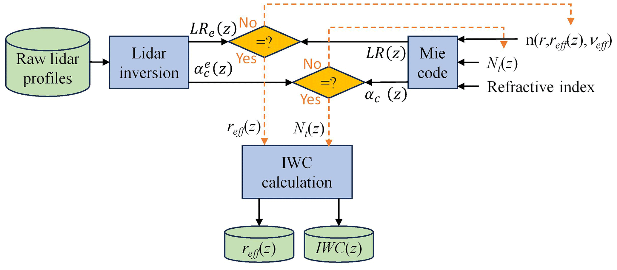
Figure 1 Flow chart of the process used to assess the effective radius r_eff and the ice water content (IWC) at each altitude z by comparing the lidar ratio (LR) and the cloud extinction coefficient ${\mathit{\alpha }}_{\mathrm{c}}^{\mathrm{e}}\left(z\right)$ derived from lidar inversion and those calculated by a Mie code. The Mie code is initialized by the normalized size number distribution n(r) calculated for each radius r, the total number N_t and the refractive index of the ice crystals. Multiple scattering is assumed to be negligible.

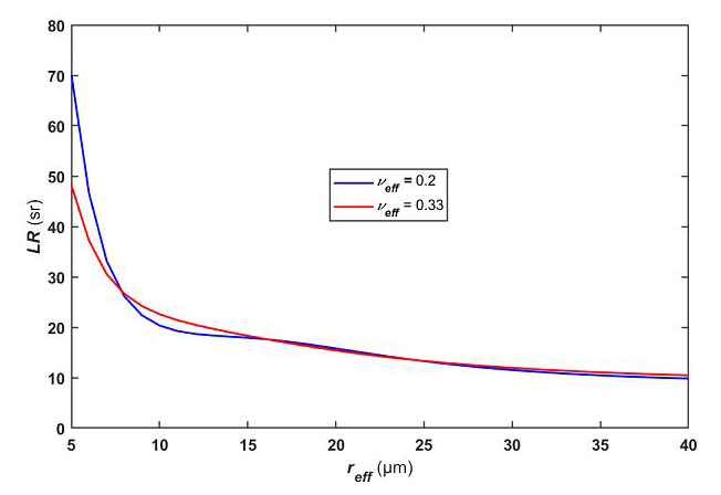
Figure 2 Variation of the theoretical lidar ratio (LR) obtained from Mie calculations as a function of the effective radius r_eff of ice crystals for two values of the effective variance ν_eff.

4 Lidar sampling

4.1 Site and meteorological synoptic conditions

The lidar measurements were obtained near Hammerfest Airport on the island of Kvaløya, which lies in a southwest/northeast trough at an altitude of ∼90 m a.m.s.l. The site is bounded by the Norwegian Sea to the west and the Barents Sea to the north. It is bordered by relief peaking at around 360 m a.m.s.l. in the northwest and relief reaching up to 1045 m a.m.s.l. in the southeast. These reliefs can therefore significantly influence flows over the site by generating wind shears and vertical mixing.

From 14 to 16 May 2016, two ridges blocked a low-pressure system between the Barents and Norwegian seas. This weather situation is illustrated by the geopotential height at 850 hPa (∼1.5 km a.m.s.l.) in Fig. 3a, where the wind field is superimposed. The first ridge is located over Greenland and extends from the mid-latitudes to the Pole, while the second ridge is located between 55 and 90^∘ E and passes over the Novaya Zemlya archipelago. The latter weakened from 16 to 17 May and thus favored the development of a low-pressure system around the Svalbard archipelago. This low then spread to the south of the Norwegian Sea. In the afternoon of 16 May, Hammerfest was on the edge of the low (Fig. 3b) with stratified cloud structures before it spread to cover the town completely by the late morning of 17 May (Fig. 3c). This led to a significant evolution of the cloud cover towards denser and precipitating clouds which appeared on the afternoon of 17 May over Hammerfest. The retrieval of the optical parameters of ice crystal relies on the lidar observations of semi-transparent frozen clouds before the arrival of denser precipitating clouds. The meteorological situation corresponds to a warm southwestern regime as named by Mioche et al. (2017).

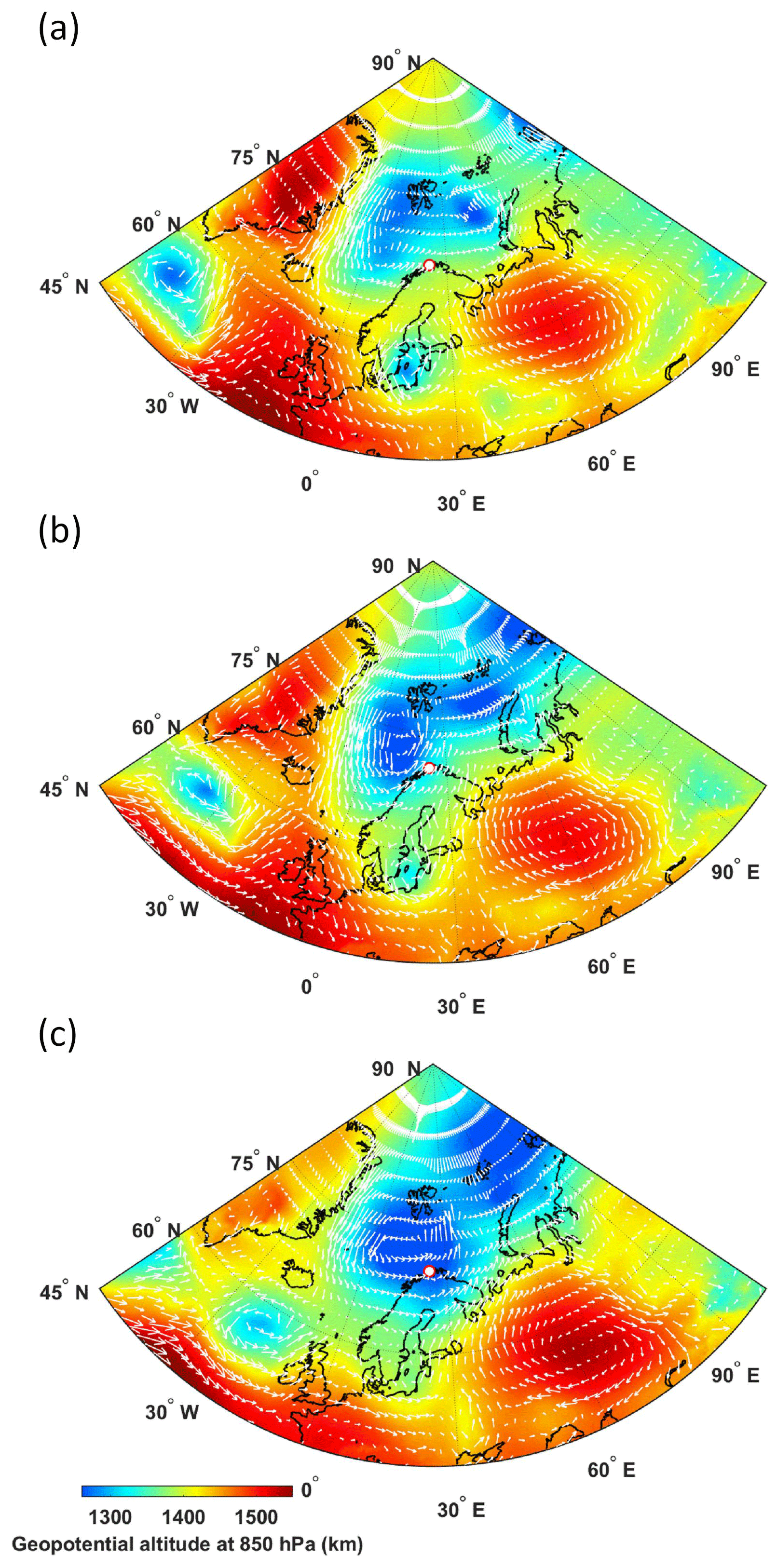
Figure 3 Geopotential height at 850 hPa on (a) 16 May 2016, 06:00 UTC, (b) 16 May 2016, 18:00 UTC, and (c) 17 May 2016, 12:00 UTC. The wind field is indicated by white arrows. The measurement site close to Hammerfest in northern Norway is indicated by a white dot with a red border.

4.2 Description of cloud structures

Just before the arrival of clouds over the measurement site, ultralight aircraft flights were made with a payload including (i) a meteorological probe to measure temperature, relative humidity, and pressure; and (ii) the Lidar for Automatic Atmospheric Survey Using Raman Scattering (LAASURS) for the retrieval of the aerosol extinction coefficient. This payload is described in Chazette et al. (2018). The vertical profiles of the temperature, relative humidity, and aerosol extinction coefficient derived from the ultralight payload on 16 May 2016, 11:30 local time (LT), are given in Fig. 4. That latter is negligible over 1.2 km above mean sea level (a.m.s.l.) (Chazette et al., 2018). The 0 ^∘C isotherm is reached at an altitude of 0.8 km a.m.s.l. with relative humidity increasing with altitude. With the advection of moist air masses over the site, the presence of cold clouds is therefore probable above 0.8 km a.m.s.l. This value is within the range of the bottom height of boundary layer mixed-phase clouds in the western Arctic (McFarquhar et al., 2007; Maillard et al., 2021). At temperatures close to those encountered here, i.e., slightly below 0 ^∘C, Luke et al. (2021) have recently shown that secondary ice formation can significantly increase the amount of ice crystals in clouds in the Arctic.

In the early afternoon of 16 May, the sky became overcast, leading to stratiform and cirrus clouds around 16:00 LT. These clouds were sampled between 16 and 17 May by the ground-based lidar. The apparent backscatter ratio (${\mathit{\beta }}_{\mathrm{app}}/\left(C\cdot {\mathit{\beta }}_{\mathrm{m}}\right)$), including the attenuation due to aerosols and clouds, and VDR time series are given in Fig. 5a. The clouds extend between ∼0.8 and 6 km a.m.s.l. and display complex structures highlighting their great heterogeneity. Some stratiform clouds may occur at 2 km altitude on 16 May and in the range 2–3 km altitude on 17 May and can be detected by a strong attenuation of the lidar signal at their tops. This might indicate the presence of supercooled liquid droplets at the top of mixed-phase clouds as often reported in the Arctic region (Mioche et al., 2017; McFarquhar et al., 2017). Higher clouds (2–6 km altitude) are also detected by the lidar. The sedimentation of ice crystals from those higher ice clouds leads to a glaciation of most of the lower liquid cloud layers (i.e., the seeder–feeder effect; Fernández-González et al., 2015).

The VDR is also highly variable temporally and vertically (Fig. 5b). The higher values (>8 %) indicate the location of frozen hydrometeors, while the lower values inside clouds (<1 %) may indicate the presence of supercooled water liquid droplets or molecular holes in the cloud structure. It is worth noting that, as the cloud-related scattering coefficient is very large compared with that of the molecules and aerosols, the VDR should not be very far from the PDR. Our observations with a vertical resolution of 15 m of liquid structures embedded in ice clouds are in agreement with previous field measurements (Rangno and Hobbs, 2001; Korolev and Isaac, 2003) which suggested that different pockets of solely water or ice in mixed-phase regions coexist with a typical scale of tens of meters. In contrast, large-scale models erroneously assume that liquid and ice phases are uniformly mixed within each model grid box (Tan and Storelvmo, 2016), with implications on the efficiency of the Wegener–Bergeron–Findeisen effect (Beesley and Moritz, 1999; Tan and Storelvmo, 2019).

The clouds are not formed over the site but over the ocean. They are then transported with a vertical gradient of the horizontal wind that generates some of the noticeable structures, such as the comma-like configuration between 00:00 and 04:00 on 17 May (Fig. 5). Between 05:00 and 07:00 LT, a cloud layer composed of supercooled droplets can be observed between 2 and 2.5 km a.m.s.l. In this case, β_app is higher than 10 with a very low VDR. We also note the probable presence of supercooled liquid droplets on 16 May between 18:30 and 19:30 LT around 2.5 km a.m.s.l. Estimating the properties of ice crystals therefore requires selecting profiles outside supercooled water pockets.

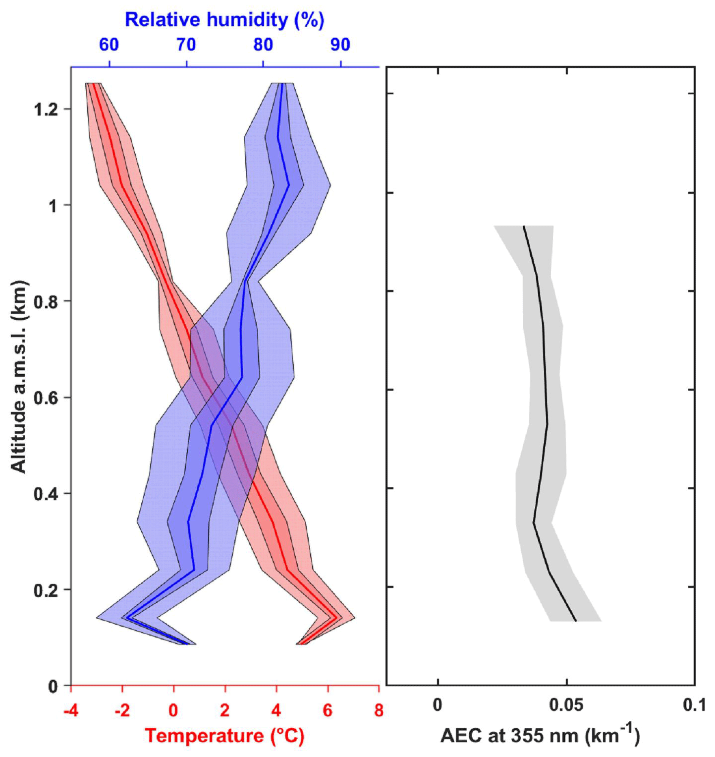
Figure 4 Vertical profiles of the temperature, relative humidity, and aerosol extinction coefficient (AEC) derived from the ultralight on 16 May 2016, 11:30 LT. The lighter-colored areas (red and blue) give the data variability in 100 m-thick atmospheric layers. The darker-colored areas give the error on temperature (red) and relative humidity (blue). The gray shaded area is the error on the AEC.

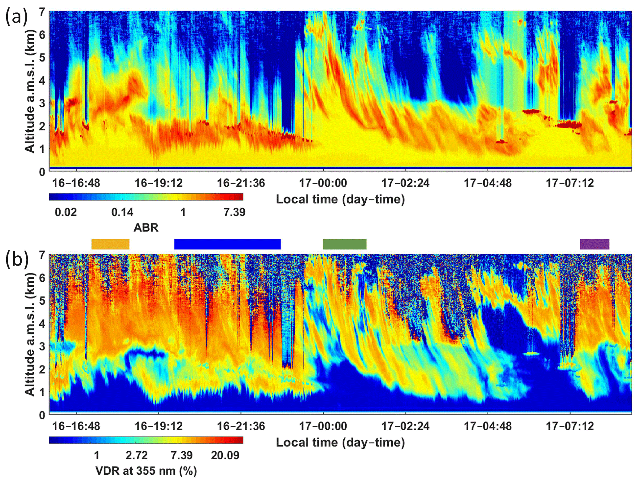
Figure 5 Time series of the (a) apparent backscatter ratio (ABR) and (b) linear volume depolarization ratio (VDR) derived from the ground-based lidar from 16 to 17 May 2016. Cases studied specifically are highlighted by the color bar above each period concerned: case 1 in orange, case 2 in blue, case 3 in green, and case 4 in violet.

4.3 Lidar-derived optical properties

We selected four cases indicated by the horizontal-colored bands in Fig. 5, when the laser beam passed through ice clouds. For each selected period we averaged the profiles over the previous time intervals to increase the signal-to-noise ratio of the lidar measurements. The lidar-derived integrated optical parameters of sampled clouds are given in Table 1 for each case. The optical properties assume a contribution from multiple scattering which is evaluated later. The consistency of the retrievals can be assessed by comparing COT_e derived from both elastic and N₂-Raman channels, which are two independent measurements. This ensures that the assumptions for molecular scattering before and after the cloud are reasonable. The difference may be ascribed to mainly two reasons: (i) the level of noise above the cloud layer that affects the boundary condition or (ii) the smaller range of the N₂-Raman channel that therefore integrates less of the upper part of the clouds. In Table 1, the “Klett” columns give the result of the Klett (1981) inversion using $\stackrel{\mathrm{̃}}{{\text{LR}}_{\mathrm{e}}}$ calculated via the N₂-Raman (Eq. 10) channel. The differences observed with the Klett inversion remain lower than 3 %. Note that the stable Klett inversion significantly reduces the errors as one moves away from the top of the cloud layer. The value of $\stackrel{\mathrm{̃}}{{\text{LR}}_{\mathrm{e}}}$ derived from the N₂-Raman channel is shown to be very stable from one case to another (between 21 and 25 sr).

In the following, we therefore use the coupling between the elastic and N₂-Raman channels to determine the vertical profiles of the LR and the vertical profiles of the extinction coefficient of ice crystals. For the four cases, the vertical profiles derived from the lidar measurements are shown in Fig. 6. $\stackrel{\mathrm{̃}}{{\text{LR}}_{\mathrm{e}}}$ are mainly between 10 and 30 sr for the cloudy structures. The higher values observed in the lowest layers are related to the transition with the atmospheric boundary layer where there can be a contribution of aerosols when the cloud structures have a very low density. ICDR is retrieved between 5 % and 15 % in the clouds, mostly below 10 %, as shown in Fig. 7 for the four cases. Such values are weak for large non-spherical ice crystals. We can therefore infer that the clouds observed are composed of small ice crystals with a rather spherical shape. It is worth noting that Nakoudi et al. (2021) found ICDR values between 10 % and 35 % for cirrus clouds over Svalbard.

Assuming that the retrieved optical properties are slightly influenced by multiple scattering and considering the processes presented in Sect. 3, we can constrain the size distribution of the ice crystals. The phase functions calculated using a Mie model coupled to the extinction profile ${\mathit{\alpha }}_{\mathrm{c}}^{\mathrm{e}}$ then allow us to evaluate the importance of multiple scattering using a Monte Carlo model. The retrieved values of η remain above 0.95 for all cases and mainly influence the top part of the clouds. We can therefore make the reasonable assumption that multiple scattering has negligible influence on our results. Note that the derived values are close to those previously determined from ground-based lidar measurements for the same type of clouds in the Arctic region ($\mathit{\eta }=\mathrm{0.92}\pm \mathrm{0.03}$) by Mariage et al. (2017).

Table 1 Equivalent integrated optical parameters at 355 nm and their uncertainties for four case studies of cloud layers: effective optical thickness (COT_e) from the elastic and N₂-Raman channels, and equivalent effective lidar ratio ($\stackrel{\mathrm{̃}}{{\text{LR}}_{\mathrm{e}}}$). The “Klett” column shows results using the Klett (1981) inversion. Altitude ranges where calculations are made are given in parentheses.

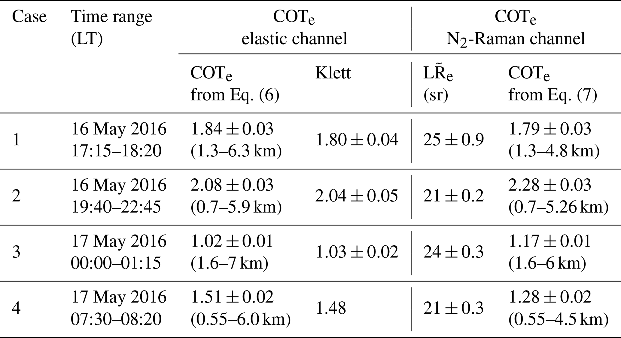
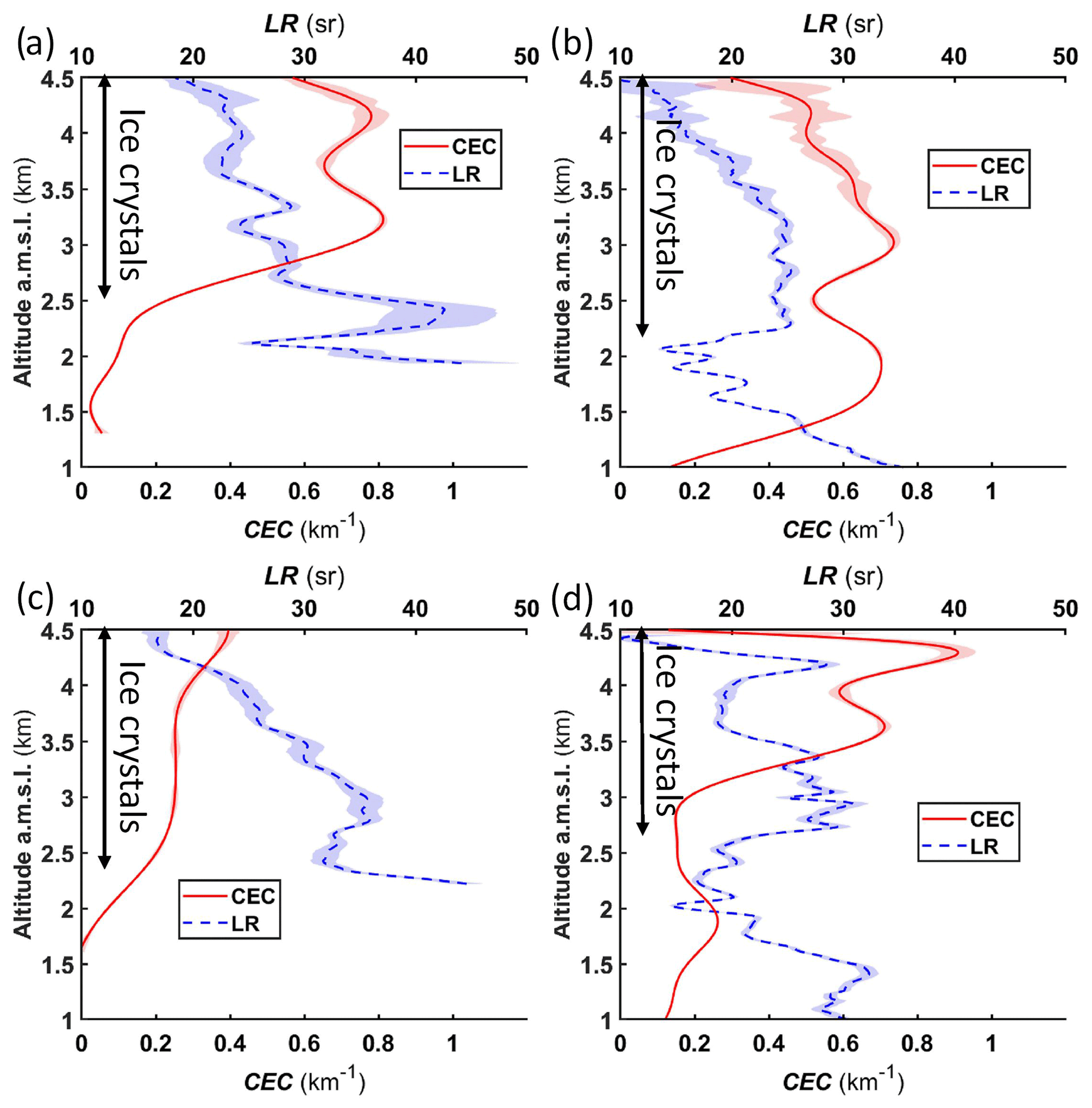
Figure 6 Vertical profiles of the lidar-derived cloud extinction coefficient (CEC) and lidar ratio (LR) on (a) 16 May 2016, 17:15–18:20 local time (LT) (case 1), (b) 16 May 2016, 19:40–22:45 LT (case 2), (c) 17 May 2016, 00:00–01:15 LT (case 3), and (d) 17 May 2016, 07:30–08:20 LT (case 4). The altitude location of ice crystals is indicated. The colored areas around the curves represent the data uncertainties.

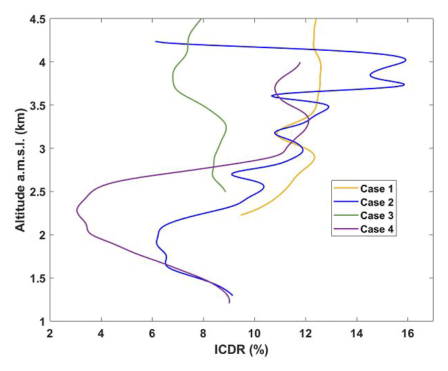
Figure 7 Vertical profiles of the lidar-derived linear ice crystal depolarization ratio (ICDR) on (a) 16 May 2016, 17:15–18:20 local time (LT), (b) 16 May 2016, 19:40–22:45 LT, (c) 17 May 2016, 00:00–01:15 LT, and (d) 17 May 2016, 07:30–08:20 LT.

5 Vertical profile of cloud microphysical properties

The vertical profiles of the effective radius r_eff and ice water content calculated as in Sect. 3 are shown in Fig. 8. Two values of ν_eff are considered (0.33 and 0.20) to evaluate potential ranges of r_eff and IWC (Fig. 8a, c, e, g). The effective radius r_eff of ice crystals presents rather small values, between 7 and 25 µm. The corresponding IWC is lower than 8 mg m⁻³, as it corresponds to small ice crystals and semi-transparent clouds. It can be noted that the value of ν_eff has little influence on r_eff and IWC because the backscatter phase functions do not change significantly (Fig. 2). The uncertainties on r_eff and IWC (Fig. 8b, d, f, h) are mainly due to the shot noise of the detection and have been calculated using a statistical error propagation. They are at most 2 µm and 0.65 mg m⁻³, respectively. The highest uncertainties are generally found at higher altitudes, where the lidar signal is most attenuated.

The values of r_eff are in the lowest range of those reported in the literature for the Arctic region by Mioche et al. (2017). They have analyzed the vertical distribution of microphysical properties, in most cases stratiform mixed-phase clouds in the boundary layer, using in situ measurements from four airborne spring campaigns in the European Arctic between 2004 and 2010. For these clouds of different nature in the southwestern regime, they showed that the ice phase dominates the microphysical properties with mean values of ∼25 µm and less than 25 mg m⁻³ for effective radius and IWC, respectively. Their analysis also revealed that large values of the liquid water content and high concentrations of small droplets may be linked to polluted situations and air mass origins from the south, leading to the lower values of ice crystal size and IWC ∼10 mg m⁻³. Our results are therefore consistent with airborne measurements on the same cloud types. Note that during PARCS, measurements were carried out over the coast of northern Norway, where the influence of local sources of pollution was not negligible (gas flaring from the Melkoya processing facility, presence of shipping activities close to Hammerfest, and transport of anthropogenic pollution from Russia) and when a plume containing biomass burning aerosols from huge forest fires in Canada reached Scandinavia (Chazette et al., 2018). The small values of ice crystal sizes and IWC found in our study may be explained by such polluted situations in comparison with clouds sampled in more pristine conditions in the high Arctic.

Similarly, McFarquhar et al. (2007) investigated the microphysical properties of single-layer stratus clouds over Barrow and Oliktok points in Alaska as part of the M-PACE (Mixed-Phase Arctic Cloud Experiment (Verlinde et al., 2007) campaign in fall 2004. They found that the effective radius of ice crystals was 25.2±3.9 µm and nearly independent of the normalized cloud altitude. Korolev and Isaac (2003) investigated mixed-phase clouds associated with frontal systems. They found that the mean volume radius of particles in ice clouds varied between 10 and 17.5 µm. Between −50 and −30 ^∘C where all cloud particles were presumably ice, the effective radius was found to be about 7 µm which is of similar magnitude to our retrievals despite higher temperatures. They argued that IWC in glaciated clouds decreased with decreasing temperature, from about 100 mg m⁻³ at −5 ^∘C to 20 mg m⁻³ at −35 ^∘C. Our observations shown in Fig. 7 do not show any evidence of such behavior for clouds encountered during PARCS. The vertical profile of IWC cannot be explained solely by the temperature values but may also be ascribed to the history of the air masses.

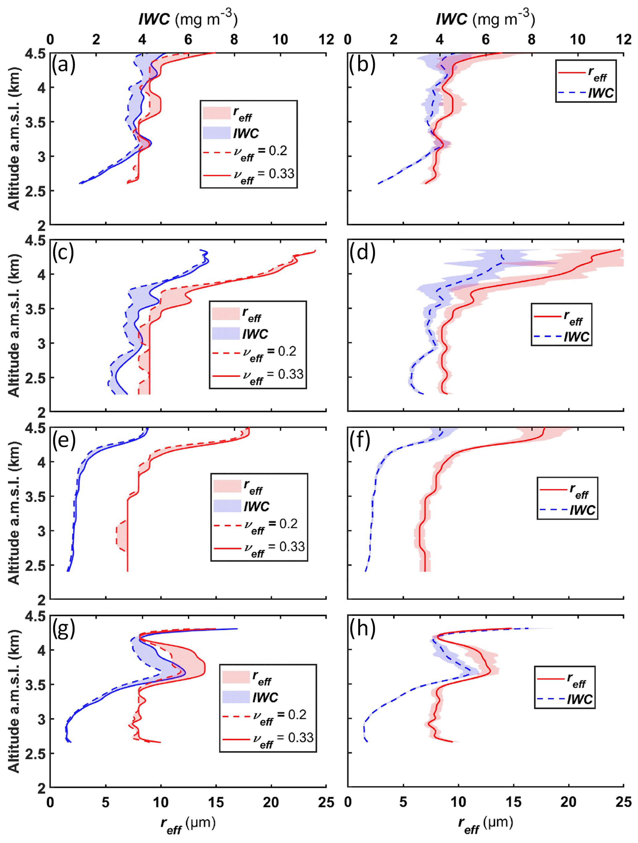
Figure 8 Vertical profiles of effective radius (r_eff) of ice crystal and ice water content (IWC) on (a, b) 16 May 2016, 17:15–18:20 LT (case 1), (c, d) 16 May 2016, 19:40–22:45 LT (case 2), (e, f) 17 May 2016, 00:00–01:15 LT (case 3), and (g, h) 17 May 2016, 07:30–08:20 LT (case 4). The left panels (a, c, e, g) represent the bias that may be linked to the choice of the ν_eff value, and the right panels (b, d, f, h) represent the shaded areas associated with the lidar measurements assuming a ν_eff value between 0.2 and 0.33.

6 Conclusion

Thin ice clouds were sampled by ground-based lidar in late spring 2016 over the Hammerfest area in northern Norway. In the presence of semi-transparent clouds with an optical thickness lower than 2 at the wavelength of 355 nm, ground-based lidar measurements allow us to differentiate the contributions of ice crystals and liquid water pockets embedded in the cloud. The clouds are located just above the atmospheric boundary layer, with a cloud base between 0.8 and 1.2 km a.m.s.l. where the temperature is below the 0 ^∘C isotherm. The inversion of the lidar profiles shows a modest level of depolarization, of the order of 10 %, with a negligible multiple scattering coefficient (<0.95 at the cloud top), suggesting that sampled ice crystals are small and of rather spherical shape. This agrees with Mie computations determining effective radii between ∼7 and 25 µm. The ice water contents are found to be lower than 8 mg m⁻³. Such small values may be ascribed to more polluted situations compared with pristine conditions in the high Arctic. It is worth noting that the uncertainties on the effective radius and ice water content are on average of 2 µm and 0.65 mg m⁻³, respectively, allowing us to follow their evolution in the cloud, as long as the lidar signal is not too attenuated.

The use of vibrational Raman measurements to constrain the elastic lidar equation allows us to remove ambiguities on the restitution of optical properties of semi-transparent ice clouds. It is an alternative approach to airborne measurements limited by the ability to sample the clouds over long periods of time. It is complementary to approaches proposing the coupling of lidar and radar measurements at 95 GHz. Its limitation is mainly on the ability of the lidar to sample the cloud layer along the line of sight and on the assumptions of sphericity of ice crystals, which have been justified by the observed values of the depolarization ratio. Our approach can nevertheless be easily extended to clouds containing non-spherical ice crystals if we consider the appropriate phase functions, which can be obtained, for instance, using T-matrix approaches applied on specific shape functions.