Suppression of precipitation bias in wind velocities from continuous-wave Doppler lidars

In moderate to heavy precipitation, raindrops may deteriorate the accuracy of Doppler lidar measurements of the line-of-sight wind velocity because their projected velocity in the beam direction differs greatly from that of air. Therefore, we propose a method for effectively suppressing the adverse effects of rain on velocity estimation by sampling the Doppler spectra faster than the time taken for a raindrop to transit through the beam. By using a special averaging procedure, we can suppress the strong rain signal by sampling the spectrum at 3 kHz. A proof-of-concept field measurement campaign was performed on a moderately rainy day with a maximum rain intensity of 4 mm h⁻¹ using three ground-based continuous-wave Doppler lidars at the Risø campus of the Technical University of Denmark. We demonstrate that the rain bias can effectively be removed by normalizing the noise-flattened 3 kHz sampled Doppler spectra with their peak values before they are averaged down to 50 Hz prior to the determination of the speed. In comparison to the sonic anemometer measurements acquired at the same location, the wind velocity bias at 50 Hz (20 ms) temporal resolution is reduced from up to −1.58 m s⁻¹ for the original raw lidar data to −0.18 m s⁻¹ for the normalized lidar data after suppressing strong rain signals. This reduction in the bias occurs during the minute with the highest amount of rain when the focus distance of the lidar is 103.9 m and the corresponding probe length is 9.8 m. With the smallest probe length, 1.2 m, the rain-induced bias is only present at the period with the highest rain intensity and is also effectively eliminated with the procedure. Thus, the proposed method for reducing the impact of rain on continuous-wave Doppler lidar measurements of air velocity is promising and does not require much computational effort.

1 Introduction

The precise determination of the wind flow plays an important role in reducing loads on critical turbine components and power variations, correcting commonly used models for wind energy assessment, improving the performance of wind turbine controllers, and improving the prediction of the potential power extracted from the wind (Davoust et al., 2014; Jena and Rajendran, 2015; Li et al., 2018; Samadianfard et al., 2020; Guo et al., 2022). Wind velocity estimation is also useful for understanding important phenomena, i.e., atmospheric boundary layer flows and wind turbulence (Van Ulden and Holtslag, 1985; Türk and Emeis, 2010; Debnath et al., 2017). Therefore, accurate measurements of wind velocity are crucial for many applications in meteorology and wind energy.

Several instruments capable of measuring the wind speed, wind direction, and turbulence in wind energy are available, each with advantages and disadvantages. In situ cup and sonic anemometers installed on meteorological masts (met masts) can only provide point measurements of wind velocity (Izumi and Barad, 1970). On the contrary, Doppler lidars can accurately and remotely sense the wind velocity by measuring Doppler spectra, although they have only a limited ability to measure turbulence due to probe-length averaging effects (Sathe and Mann, 2013). For more than a decade, Doppler lidars have been widely used as more and more reliable, valuable, and active optical remote-sensing instruments with easier and cost-effective deployment. Both scanning lidars and profiling lidars (Mann et al., 2017; Menke et al., 2020; Gottschall et al., 2021) with good spatial and temporal resolutions (Henderson et al., 1991; Aoki et al., 2016) have been applied to estimate wind resources both onshore (Bingöl et al., 2009) and offshore (Sempreviva et al., 2008; Peña et al., 2009; Viselli et al., 2019; Elshafei et al., 2021).

Apart from the aforementioned advantages, Doppler lidars have the potential to reduce loads on turbine blades and towers through their capacity to foresee the incoming gusts and flow (Bossanyi et al., 2014; Bos et al., 2016) and improve wind turbine control (Mikkelsen et al., 2013; Schlipf et al., 2015; Zhang and Yang, 2020). Doppler lidars can also be applied to study atmospheric turbulence along the span of a suspension bridge (Cheynet et al., 2016) and to study the turbulent wind field in the near-wake region of a tree (Angelou et al., 2022). In order to improve the measurement accuracy of lidars, Wildmann et al. (2020) reduced the volume-averaging effect on the retrieval of the wind flow statistics by ground-based Doppler lidars (see also Sathe and Mann, 2013). Brinkmeyer (2015) suggested that a low-coherence Doppler lidar approach using a pseudo-random broadband laser source could be used to obtain a confined measurement volume. It is self-evident that the precise determination of the wind velocity with Doppler lidars is paramount for many applications in wind energy.

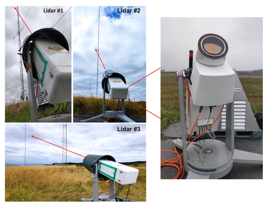
Figure 1 The three CW lidars were pointed at a common focus point close to a sonic anemometer on a met mast at DTU Risø campus.

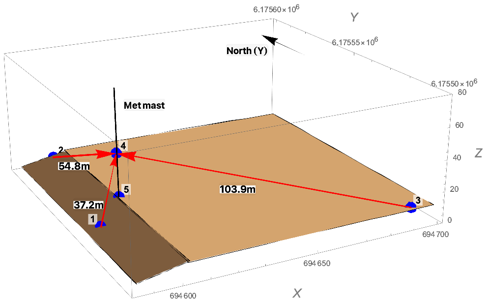
Figure 2 Three-dimensional view of the experimental setup at DTU Risø campus. The blue points labeled 1, 2, and 3 are the three CW Doppler lidars. They are focused on the common point 4, which is 1 m north of the sonic anemometer at a height of 31 m above the ground. Point 5 is the base of the met mast. The solid black line indicates the met mast.

Doppler lidar measurements of wind velocity can be influenced by heavy rainfall because the projected velocity of raindrops in the propagation direction of the lidar beam is different from the line-of-sight wind velocity. A synergetic approach proposed by Träumner et al. (2010) combined radar and vertically scanning lidar measurements to estimate the vertical wind velocity and the raindrop size distribution during rain episodes. Later, by using a velocity-azimuth display (VAD) scanning technique, the wind speed and rainfall speed were simultaneously retrieved in Wei et al. (2019) by fitting the two-peak spectrum with a two-component Gaussian model. The spectral peak close to 0 m s⁻¹ is the Doppler signal of the vertical wind speed, which can be easily recognized in this scenario. Aoki et al. (2016) and Wei et al. (2021) proposed an iterative deconvolution method to retrieve the raindrop size distribution during rain by using a vertically pointing coherent Doppler lidar.

Table 1 Summary of the measurement parameters of the three CW lidars. Note that the geographic beam direction is given relative to the north and clockwise is positive.

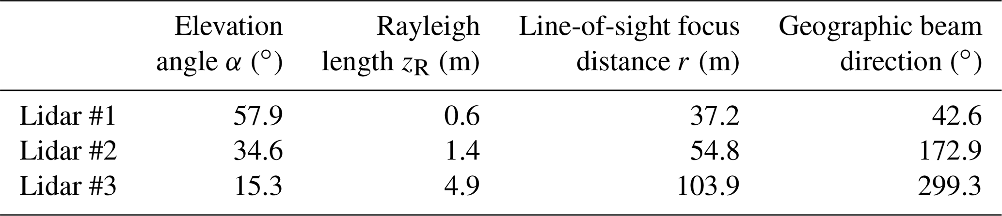
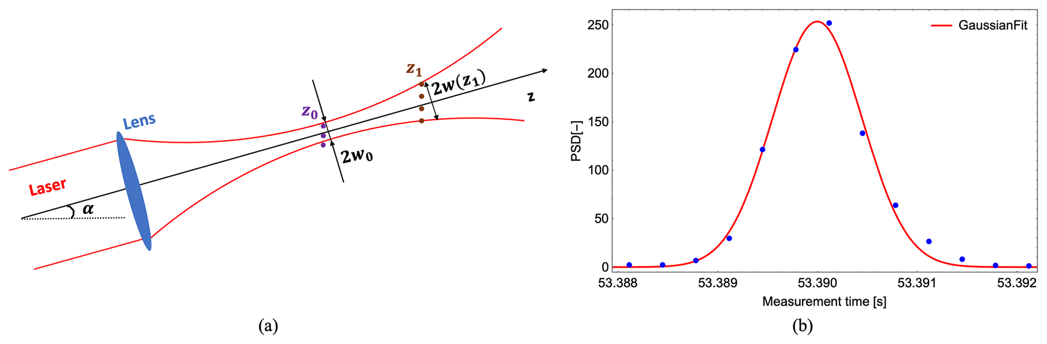
Figure 3 An illustration of raindrops falling through a focused laser beam. (a) Raindrops cross the laser beam at the random positions z₀ and z₁, where z₀ is the focus point. (b) The raindrop-induced Doppler signal during a raindrop's passage through the beam follows a Gaussian distribution since the laser beam's transverse intensity profile is Gaussian (Harris et al., 2001; Jin et al., 2022).

However, for Doppler lidars which do not point vertically, the line-of-sight wind velocity is not close to zero and it is difficult to distinguish the part of the signal that originated from raindrops or from air-following aerosols. Therefore, the purpose of the present study is to provide a proof-of-concept experimental investigation of a method we propose for suppressing the precipitation signal in the aerosol signal in order to reduce the rain-induced bias in the velocity estimation.

A field measurement campaign was carried out at Risø, where three coherent continuous-wave (CW) Doppler lidars (Mikkelsen et al., 2017) were deployed to point towards a common focus point very close to a mast-mounted sonic anemometer at 31 m height. The lidars had different elevation angles, focus distances, and probe lengths. Therefore, it was possible to investigate the influence of these parameters on the performance of the post-processing method. The basic idea was to sample Doppler spectra rapidly, i.e., at 3 kHz, which allowed us to detect when a raindrop was in the beam. Measurements from a sonic anemometer were used as a reference to compare with the estimated line-of-sight wind velocities from the three lidars before and after suppressing the rain Doppler signals in the Doppler spectra. The corresponding rain characteristics were retrieved from a ground-based disdrometer (Tilg et al., 2020) near the meteorological mast.

Section 2 introduces the field campaign and elaborately describes the instruments used. In Sect. 3, the measurement results from the sonic anemometers and the disdrometer are presented. The principle of Doppler spectral processing to retrieve the line-of-sight wind velocity as well as our proposed method to suppress strong rain signals are presented in detail in Sect. 4. Section 5 shows a comparison between the lidar and sonic anemometer measurements in terms of the 50 Hz and 1 min wind velocity time series obtained with and without the suppression of the rain signals. The most important findings of our study are summarized in the “Conclusion” (Sect. 6).

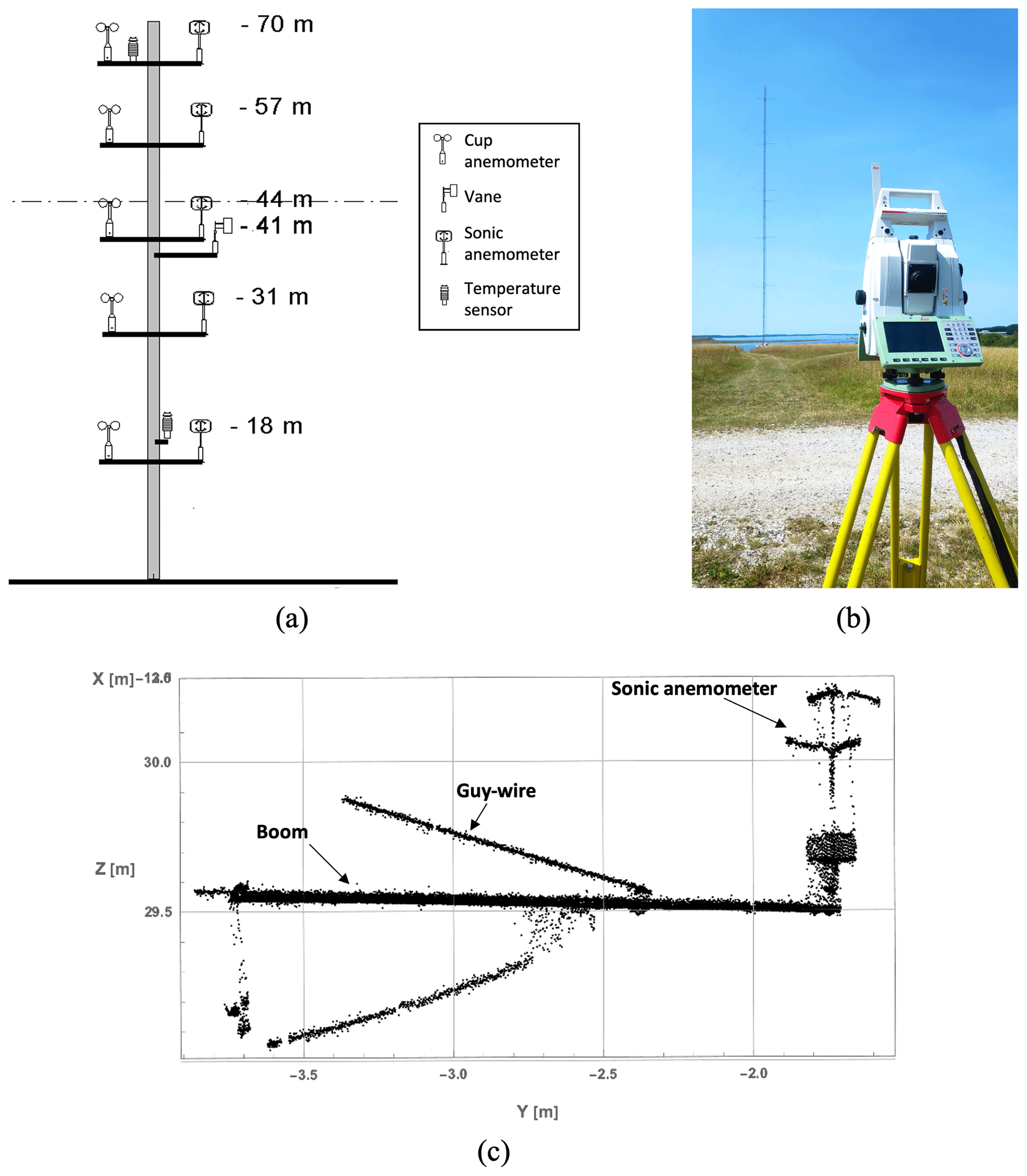
Figure 4 Orientation calibration of the sonic anemometers on the met mast. (a) A sketch of the V52 meteorological mast with the instrumentation. The dashed line indicates the hub height of the DTU V52 wind turbine. (b) Leica total station (Leica Geosystems, 2023). (c) Cloud points scanned by the sonic anemometer at a height of 31 m.

2 Instrumentation

2.1 The WindScanner system

In order to validate the method used to reduce the influence of the precipitation on the estimated wind velocity, we conducted a field experiment at the Risø campus of the Technical University of Denmark (DTU), as shown in Fig. 2. The surrounding terrain is flat and agricultural. A short-range WindScanner system that uses three CW Doppler lidars (Fig. 1) developed by DTU Wind and Energy Systems was used to measure the wind field (Vasiljević et al., 2017; Mikkelsen et al., 2020). The three lidars employ a dual-prism beam scanner, enabling them to orient the beam in any direction within ±61^∘ of the adjustable center axis (Sjöholm et al., 2014; Mikkelsen et al., 2008). The direction of the line of sight of each lidar is steered by two prism motors and a focus motor controls the measurement location along the beam for these lidars. For this campaign, the sampling frequency of spectra was set to be 3 kHz. A central master computer is used to synchronize the short-range wind lidars as they scan the same pattern in space simultaneously; however, all three lidars were focused on one static point in this investigation.

The three ground-based lidars were focused on a point 1 m north of a sonic anemometer (USA-1, METEK) located 31 m above the ground. The lidar heads were covered with green rain barrels to stop raindrops from covering the windows of the lidars (Fig. 1). The reason for using three lidars was to investigate the influence of different probe lengths and different elevation angles on the performance of the method to suppress rain signals. The full width at half maximum (FWHM) of the Lorentzian weighting function or the probe length can be approximated as (Sathe and Mann, 2013)

$$\begin{array}{}\text{(1)}& \text{FWHM}=\mathrm{2}\cdot z_{\mathrm{R}}=\mathrm{2}\cdot {\displaystyle \frac{\mathit{\lambda }\cdot r^{\mathrm{2}}}{\mathit{\pi }{a}_{\mathrm{0}}^{\mathrm{2}}}},\end{array}$$

where z_R is the Rayleigh length, defined as the distance from the focus point to where the cross-sectional area of the laser beam is doubled (Angelou et al., 2012b); r is the distance from the lidar to where the beam is focused; λ is the laser wavelength, which is 1.565 µm; and a₀ is the e⁻² intensity radius of the laser beam at the lidar telescope, which is about 33 mm. The measurement parameters of the three lidars are summarized in Table 1, and a three-dimensional view of the configuration of the three lidars is depicted in Fig. 2. Lidar #1 is placed on a slope, so it has a relatively big elevation angle of about 58^∘ but the smallest probe length of 1.2 m compared with lidars #2 and #3. The measurement period of the three lidars was from 15:12 to 23:29 UTC+1 on 27 September 2022. All times mentioned in the paper are UTC+1.

Figure 5 The Thies laser precipitation monitor (LPM) at DTU Risø campus.

Table 2 Technical details of the Thies laser precipitation monitor (LPM) (Clima, 2023).

The backscattered light mixed and amplified by the local oscillator is sampled at a rate of 120 MHz, and Doppler spectra containing 512 frequency bins are calculated by a fast Fourier transform (FFT) with a frequency resolution of $\left(\mathrm{120}\mathrm{MHz}\right)/\mathrm{512}=\mathrm{234.4}$ kHz. The wind speed resolution is calculated from this frequency resolution and the laser wavelength λ, yielding $(\mathrm{1.565}\mathrm{\mu }\mathrm{m}/\mathrm{2})\cdot \left(\mathrm{234.4}\mathrm{kHz}\right)=\mathrm{0.183}$ m s⁻¹. In order to determine the sign of the line-of-sight velocity, the in-phase/quadrature-phase (IQ) detection method (Abari et al., 2014) is employed, which mixes the received signal with two local oscillator signals phase shifted by 90^∘ relative to each other. Subsequently, block averaging of 78 spectra results in a final sampling period of $\mathrm{512}\cdot \mathrm{78}/\left(\mathrm{120}\mathrm{MHz}\right)=\mathrm{0.33}$ ms, corresponding to a spectrum rate of 3 kHz. Therefore, each lidar will provide 180 000 spectra every minute. Additionally, Bartlett's method is used to obtain the power spectral density (PSD) of each spectrum (Press et al., 1988, Chap. 13), which is the square of the absolute value of the FFT of the detector's time series. The median method (Held and Mann, 2018) is employed to determine the wind velocity.

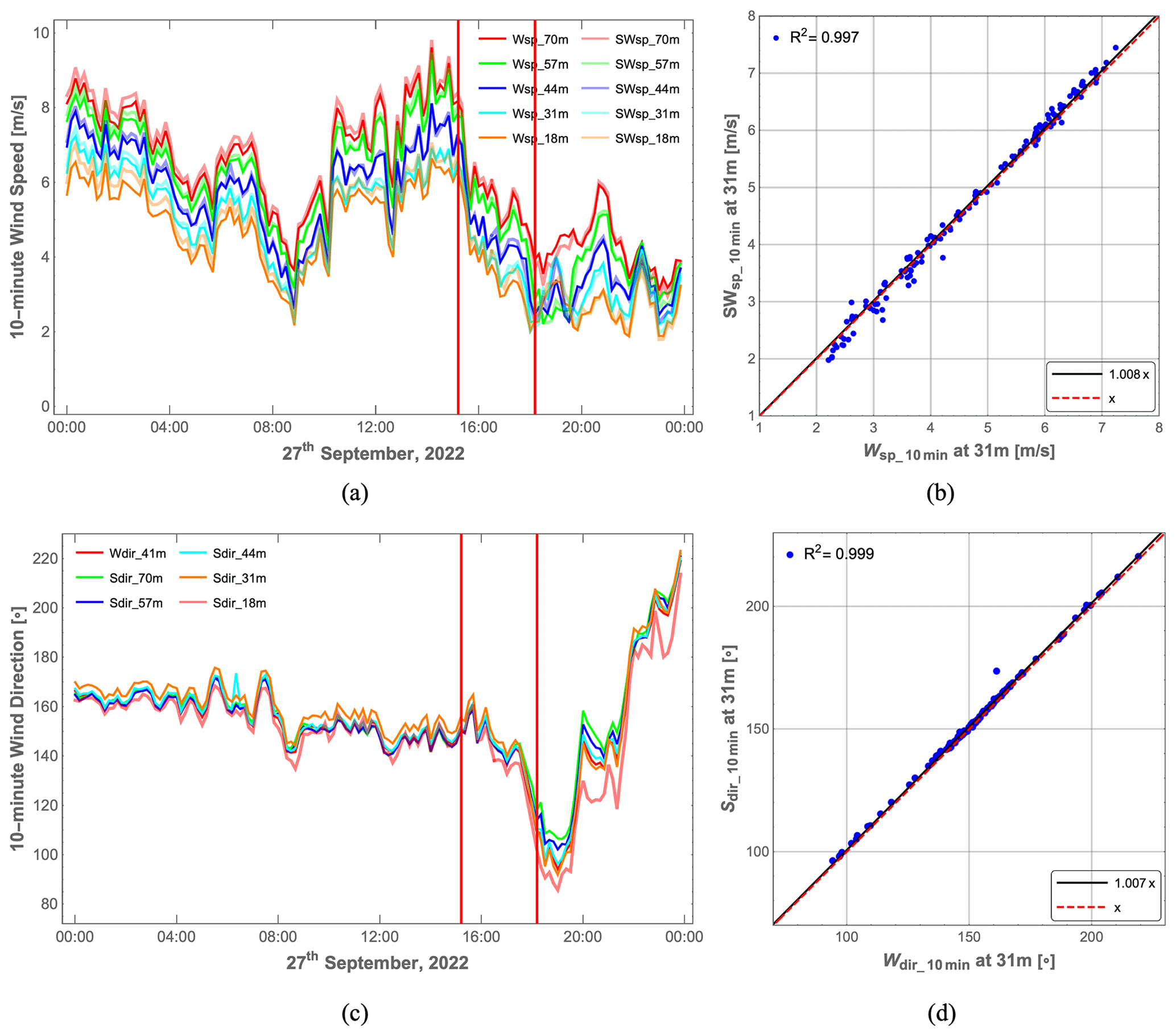
Figure 6 Comparison of 10 min wind measurements from the wind vane and the sonic and cup anemometers at several vertical heights. (a) Ten-minute wind speeds from the sonic (SW_sp) and cup (W_sp) anemometers. (b) Ten-minute wind directions from the sonic anemometers (S_dir) and the wind vane (W_dir). (c, d) Linear regression of 10 min wind speed on direction. The two red lines mark the start and end of the comparison period between the lidar and sonic anemometer data (from 15:12 to 18:11 UTC+1).

The transit time t of a raindrop through the beam is defined as the time taken for the raindrop to exit the laser beam after entering it, which is calculated by dividing its falling path l by its downfall speed V_f as follows:

$$\begin{array}{}\text{(2)}& t={\displaystyle \frac{l}{V_{\mathrm{f}}}}={\displaystyle \frac{\mathrm{2}w\left(z\right)}{\cos \left(\mathit{\alpha }\right)\cdot V_{\mathrm{f}}}},\end{array}$$

where w(z) is the beam width at position z (measured from the focus) along the beam and α is the elevation angle of the laser beam. The beam transit time will be the shortest when w(z) is the smallest and V_f is the largest. This occurs when a large raindrop falls through the laser beam's focus (position z₀ in Fig. 3a) with a maximum falling speed V_fmax of 9 m s⁻¹ (from the disdrometer measurement in Fig. 7b), which is

$$\begin{array}{}\text{(3)}& t_{\mathrm{s}}={\displaystyle \frac{\mathrm{2}{w}_{\mathrm{0}}}{\cos \left(\mathit{\alpha }\right)\cdot V_{\text{fmax}}}},\end{array}$$

where $w_{\mathrm{0}}=\frac{r\cdot \mathit{\lambda }}{\mathit{\pi }\cdot a_{\mathrm{0}}}$ is the beam waist and a₀=33 mm is the effective radius of the telescope. For lidar #1 with a beam waist of 0.56 mm and an elevation angle of 57.9^∘, the shortest beam transit time is 0.234 ms, while it is 0.362 ms for lidar #3 with a beam waist of 1.57 mm and an elevation angle of 15.3^∘. Most often, however, the transit time of raindrops is longer than the aforementioned shortest time if their paths are away from the lidar focus (position z₁ in Fig. 3a) and if they fall slower than V_fmax. In this study, it is reasonable to set the spectral sampling frequency to 3 kHz so that the sampling period for a spectrum (0.333 ms) is shorter than the beam transit time of raindrops. Therefore, the rare instances where a raindrop resides in the beam can be identified (raindrop-induced Doppler signals are detected in several successive spectra in Fig. 3b) and suppressed based on the lidar measurements.

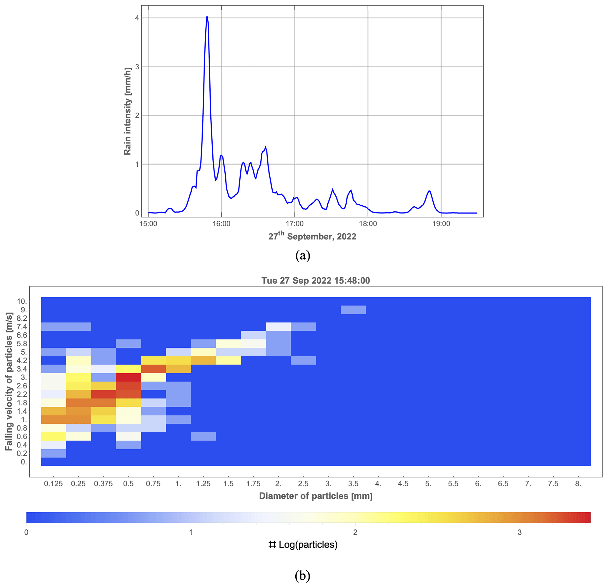
Figure 7 Rain event from 15:00 to 19:30 UTC+1 on 27 September 2022 measured by the Thies laser precipitation monitor disdrometer. (a) One-minute rain intensity. (b) Distribution of the measurements of vertical falling speed and mass-weighted mean diameter obtained during the minute (15:48) with the highest rain intensity (color coded).

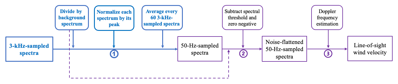
Figure 8 Processing block diagram for the rain-suppressing normalization method (the solid lines from ➀ to ➂) to estimate the wind velocity based on 3 kHz sampled Doppler spectra. The processing block diagram for Doppler spectra obtained at lower frequencies that do not resolve individual raindrops (like 50 Hz) reduces to the purple path and the “Divide background spectrum” block (as indicated by the dashed purple line before ➁).

2.2 METEK sonic anemometer

The meteorological mast location is approximately 120 m northwest of the DTU V52 wind turbine and its base is 7.3 m above the sea surface (Fig. 2). There are five sonic anemometers (USA-1, METEK) on booms facing north and five cup anemometers (P2546 A from WindSensor) on booms facing south, which are placed 18, 31, 44, 57, and 70 m above the terrain (Fig. 4). The sampling frequency of the sonic anemometers was 50 Hz. Furthermore, the mast is instrumented with a vector wind vane (W200P from Kintech Engineering) at 41 m and two air temperature sensors (Pt 100, developed by DTU) mounted at 18 and 70 m, respectively. In order to test the consistency of the mast wind measurements, the available sonic and cup anemometer observations at different heights are compared in the following section. The sonic anemometer at 31 m is used as a reference for further comparison with the radial wind velocities detected by the three lidars.

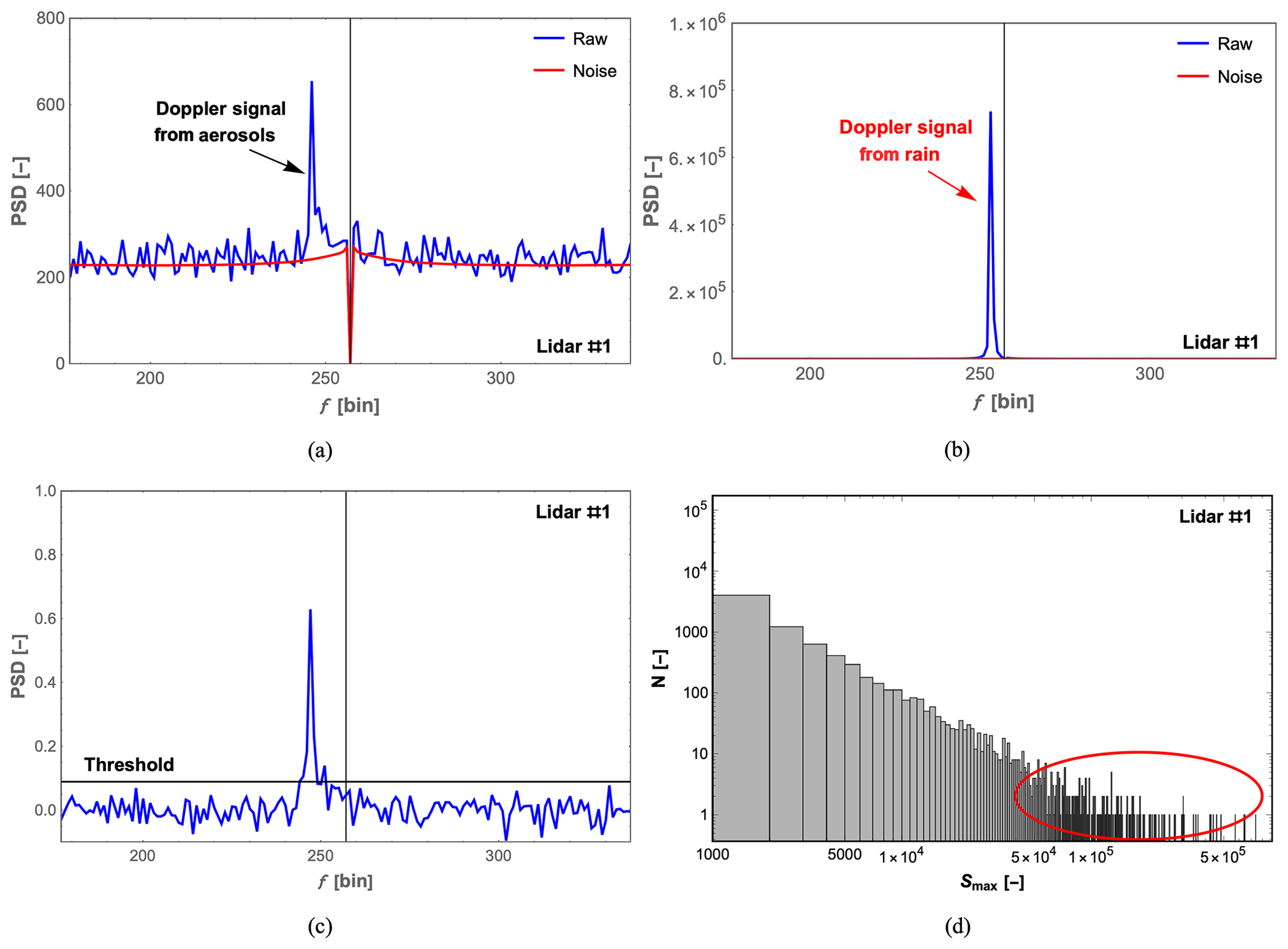
Figure 9 Examples of representative Doppler spectra measured during the moderate-rain minute (15:48 UTC+1) with the highest rain intensity. (a) A 3 kHz sampled spectrum containing only the wind signal (blue) and the mean background spectrum (red). (b) A 3 kHz sampled spectrum containing rain signal (blue) and the mean background spectrum (red). (c) A noise-flattened 50 Hz sampled spectrum and its spectral threshold. (d) Histogram of the maximum spectral energies S_max of 180 000 raw spectra obtained during the same minute, with a red circle marking the strongest rain signals. The vertical black line in (a) to (c) indicates zero Doppler shift at frequency bin 257.

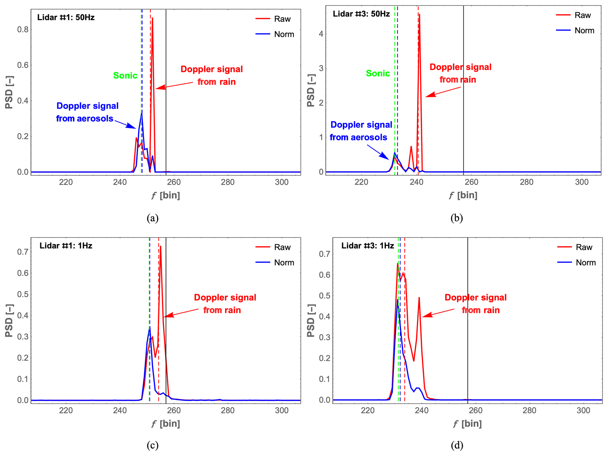
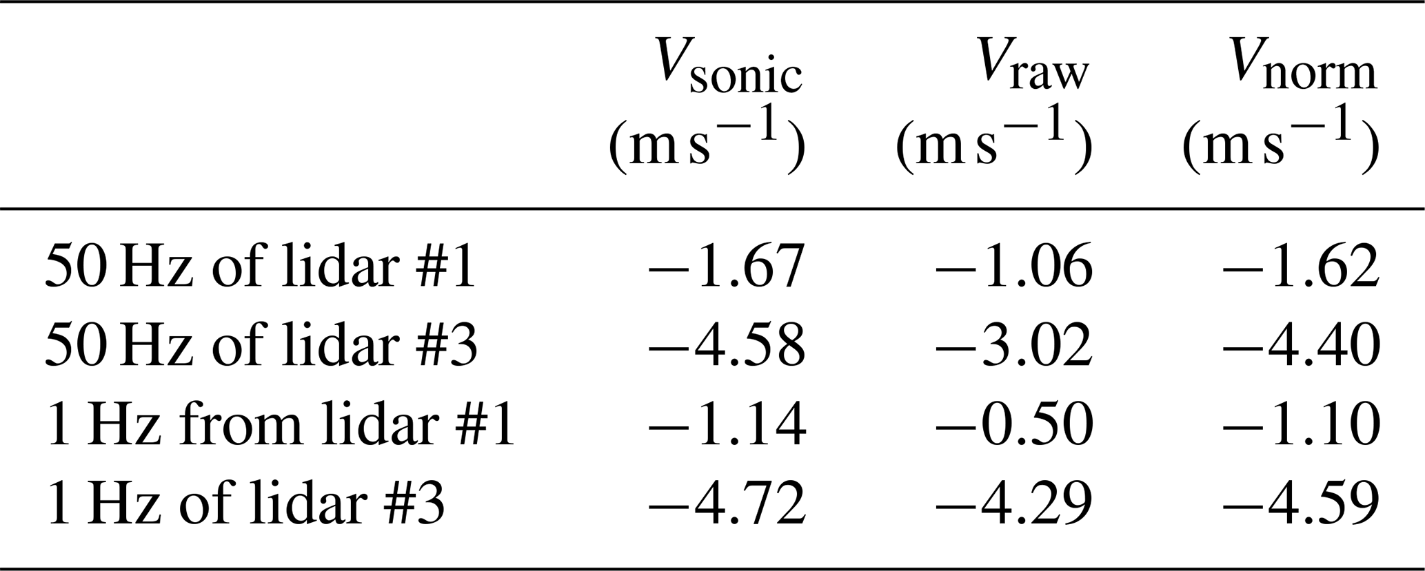
Figure 10 Doppler spectra, containing both wind and rain Doppler signals, that were obtained by two lidars during the moderate-rain minute (15:48 UTC+1) and have undergone rain signal suppression (labeled “Norm”, short for normalization) compared with the same spectra that have not undergone rain signal suppression (labeled “Raw”). (a, b) Spectra sampled at 50 Hz for lidar #1 and #3. (c, d) Spectra sampled at 1 Hz for lidar #1 and #3. The dashed red and dashed blue lines represent the median frequency bins of the raw and the normalized Doppler spectra, which are used to derive the line-of-sight wind velocity. The dashed green line indicates the sonic anemometer wind velocity and the solid black line indicates zero Doppler shift at frequency bin 257.

Table 3 Estimated wind velocities from lidar data with (V_norm) and without (V_raw) normalization and from the sonic anemometer (V_sonic). The velocities were estimated from 50 and 1 Hz sampled spectra of lidar #1 and lidar #3 obtained during the moderate-rain minute (15:48 UTC+1).

In this step, it is also important to get the accurate orientation of the sonic anemometer. For this purpose, the azimuth angle of the boom is considered as the direction offset of the sonic anemometer relative to the north. Here, a Leica total station (Fig. 4b) was used to scan the sonic anemometer at 31 m height, the boom at the same height, and the three lidars. The scanning results from the sonic anemometer at 31 m height are presented in Fig. 4c. The azimuth angle of the boom with respect to the north is 13.2^∘ in the UTM32 zone and the tilt angle of the sonic anemometer with respect to the vertical is 1.9^∘, which will be used to derive the unit vectors when projecting the reference sonic anemometer velocity onto the directions of the three lidar beams. Consequently, the unit vectors of the three lidar beams are [−0.36, −0.39, −0.85], [−0.10, +0.82, −0.57], and [+0.84, −0.47, −0.26].

2.3 Disdrometer measurements

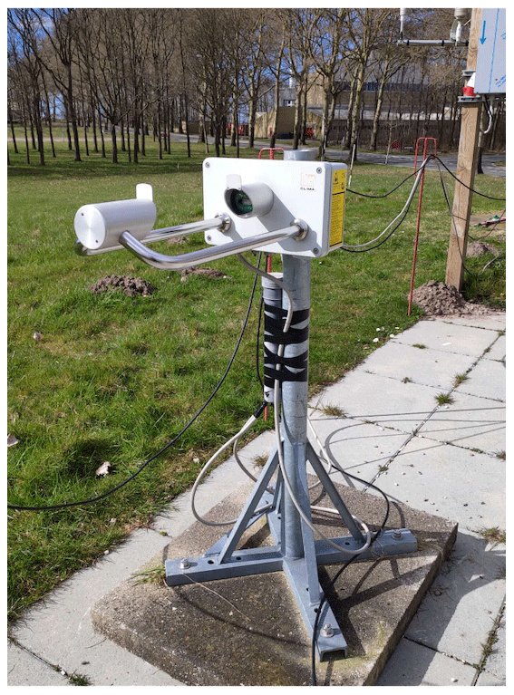
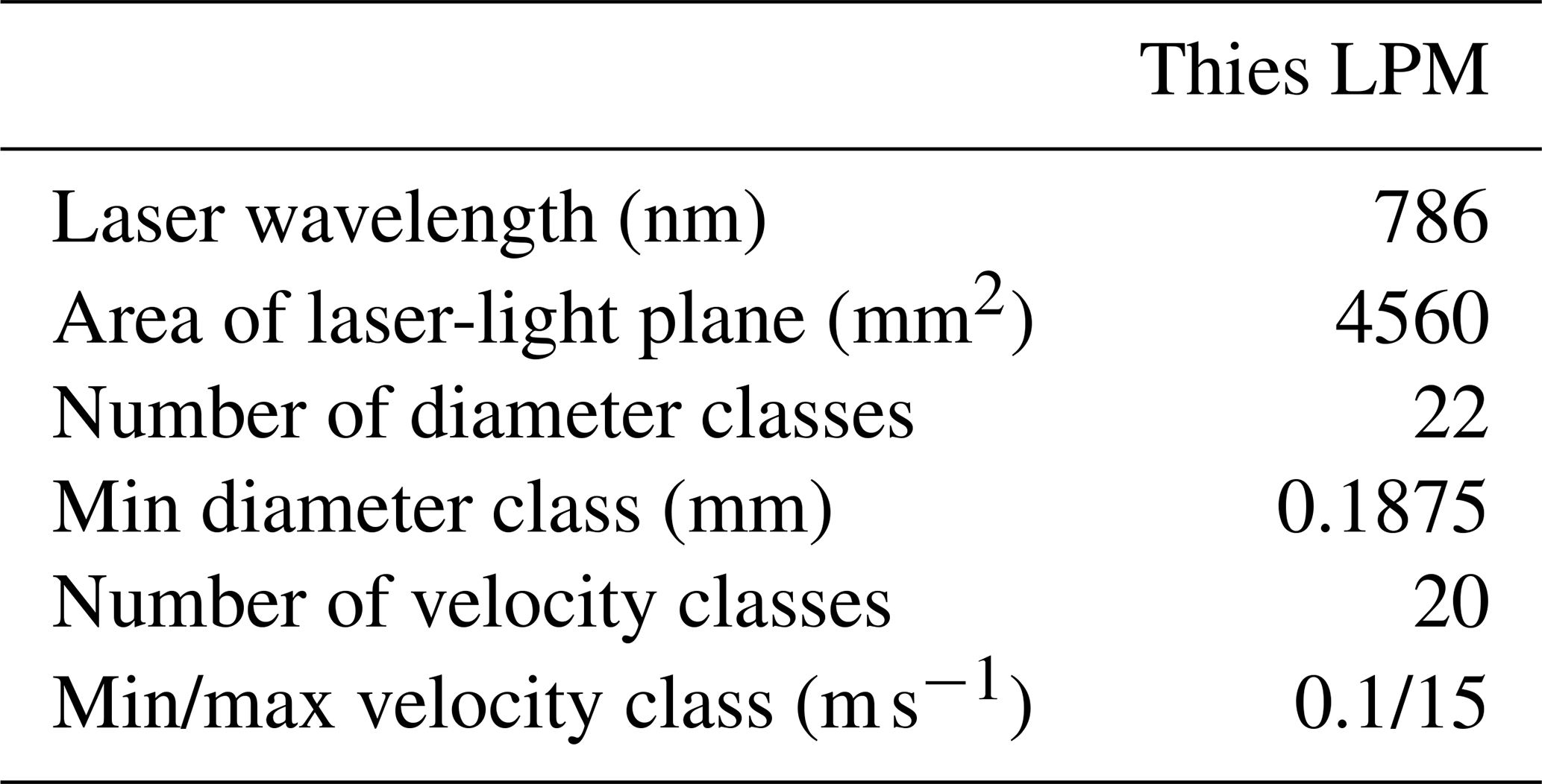
The falling velocities and diameters of the raindrops were measured by a laser optical disdrometer (laser precipitation monitor, LPM, manufactured by Thies) with a transmitter head that emits a horizontal laser-light plane and a receiver head that detects the emitted laser light (Fig. 5). When a raindrop intersects the laser beam, it attenuates the power of the transmitted laser light by a specific magnitude as a function of the falling velocity and the diameter. After the application of a proprietary algorithm, the measured raindrops are classified into specific velocity and diameter classes, which are outputted with a temporal resolution of 1 min. Here, the raindrop diameter is given as the equi-volume sphere diameter (Angulo-Martínez et al., 2018). Some technical details for the Thies LPM disdrometer are given in Table  2. This disdrometer was about 20 m north of the met mast.

3 Sonic anemometer and disdrometer data

3.1 Ten-minute-averaged sonic anemometer data

Before analyzing the sonic anemometer and lidar data, the sonic and cup anemometer wind speeds as well as the sonic anemometer and vane wind directions at different heights were compared. In Fig. 6a and b, we show that the 10 min averaged wind speeds from the sonic and cup anemometers are in good agreement at all heights, including at a height of 31 m, where the lidars were measuring. The slope of the linear regression is 1.008, with a coefficient of determination R² equal to 0.997, which shows that the wind speeds measured by the sonic anemometers agree well with those measured by the cup anemometers (with only a 1 % difference). The same conclusion can be drawn for the wind directions in Fig. 6c and d. Also, the mean absolute difference in wind speed between the sonic and cup anemometers at 31 m height is 0.11 m s⁻¹, and the mean absolute difference in wind direction between the sonic anemometer at 44 m and the vane at 41 m height is 1^∘. For further comparison with the lidar data, the three unit vectors describing the direction of the line of sight are used to project the wind vector measured by the sonic anemometer onto the lidar's line of sight, as mentioned in Sect. 2.2.

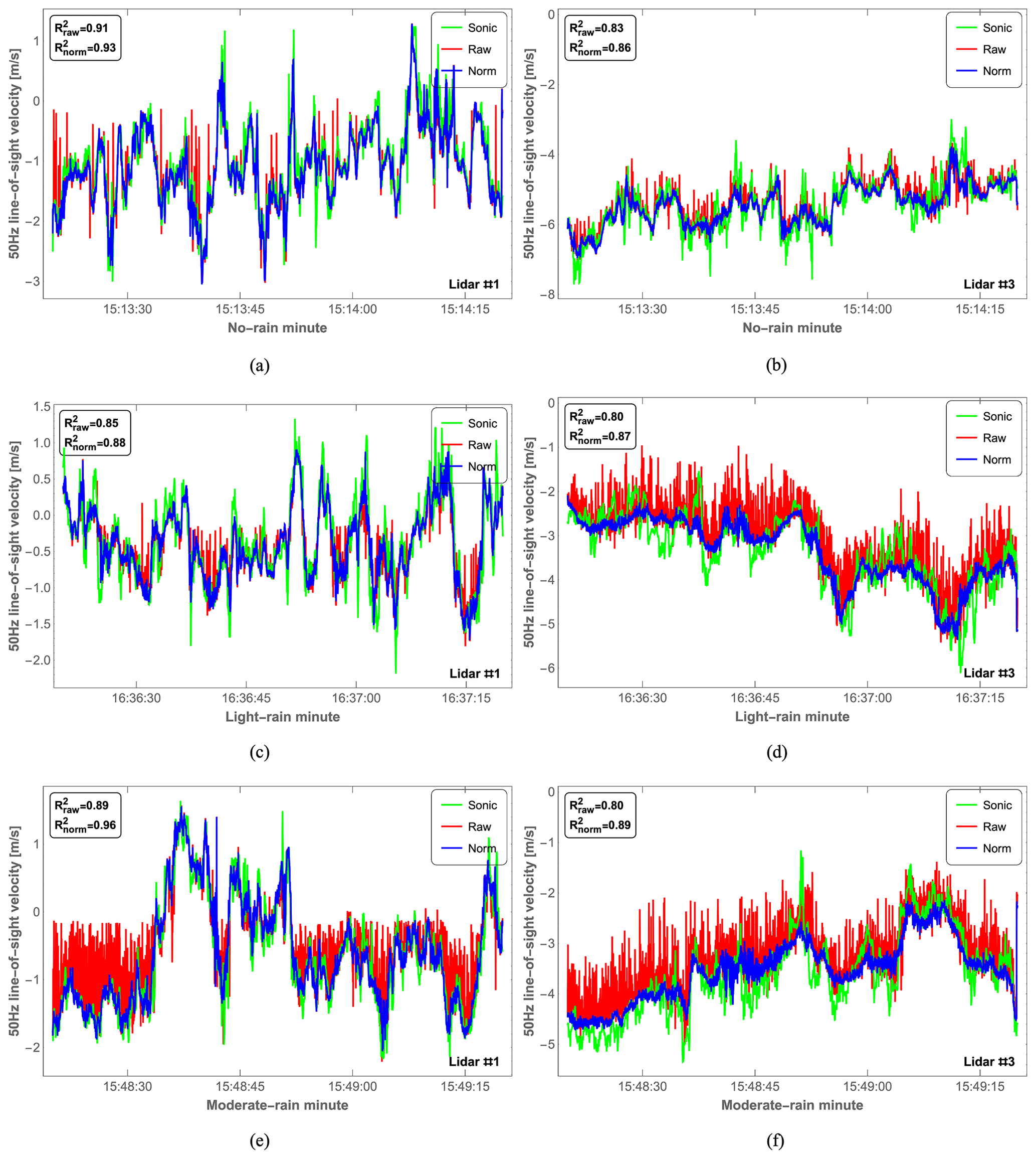
Figure 11 Comparison of 50 Hz radial wind measurements obtained by sonic anemometer (green) and lidars (red and blue) during the no-rain, light-rain, and moderate-rain minutes from top to bottom, respectively. (a, c, e) Lidar #1 (probe length of 1.2 m). (b, d, f) Lidar #3 (probe length of 9.8 m). The raw and normalized lidar data are shown in red and blue, respectively.

Table 4 Biases between the 1 min averaged wind velocity based on 50 Hz data given by the sonic anemometer and the corresponding velocities given by lidar #1 (probe length of 1.2 m) with (norm) and without (raw) normalization during 3 min with different rain intensities. The rain intensities during the light-rain and moderate-rain minutes were 1 and 4 mm h⁻¹, respectively.

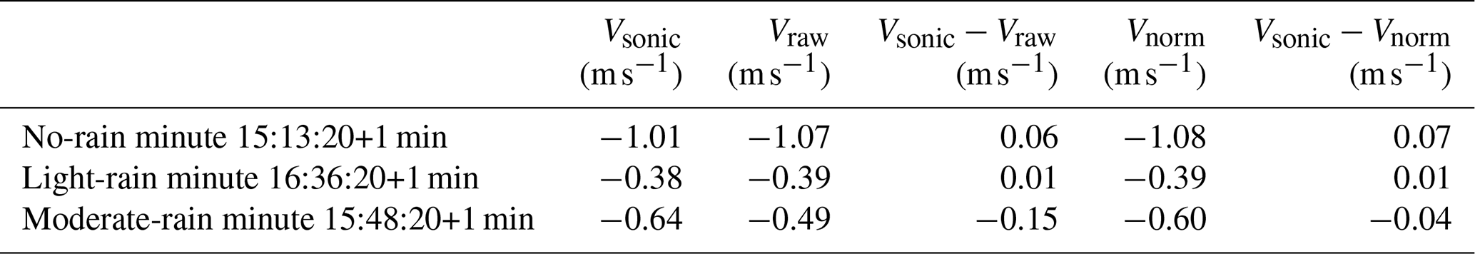
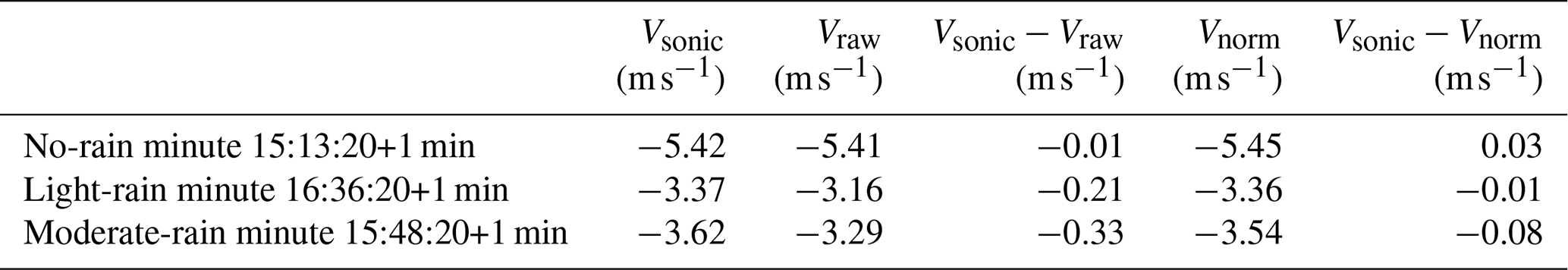
Table 5 Biases between the 1 min averaged wind velocity based on 50 Hz data given by the sonic anemometer and the corresponding velocities given by lidar #3 (probe length of 9.8 m) with (norm) and without (raw) normalization during 3 min with different rain intensities The rain intensities during the light-rain and moderate-rain minutes were 1 and 4 mm h⁻¹, respectively.

The experiment started at 15:12 UTC+1 and stopped after 3 h of measurements. This is because the measurement volumes entered the wake of the Vestas V52 wind turbine. Whether the turbine wake would have affected the measurements is unknown, but we wanted to avoid this complication. From 15:12 to 18:11 (marked by the two red vertical lines in Fig. 6), the 10 min mean wind speed obtained from the sonic anemometer at 31 m is in the interval [2.02 m s⁻¹, 6.59 m s⁻¹], while the wind direction is in the interval [110.9^∘, 164.8^∘].

3.2 One-minute disdrometer data

The 1 min averaged rain intensity from 15:00 to 19:30 UTC+1 measured by the Thies disdrometer is shown in Fig. 7a. It started to rain at 15:15, reached the highest precipitation rate of about 4 mm h⁻¹ at 15:48, and stopped after 19:00. Moderate rain is defined as a precipitation rate between 2.6 and 7.6 mm h⁻¹ (Glossary of Meteorology, 2000). The selected comparison period from 15:12 to 18:11 includes no-rain, light-rain (the precipitation rate is smaller than 2.5 mm h⁻¹), and moderate-rain minutes, which enables us to investigate the performance of our proposed method for different precipitation categories. During the highest rain intensity period, most of the raindrops have mass-weighted mean diameters smaller than 2 mm and falling velocities smaller than 6 m s⁻¹, as shown in Fig. 7b.

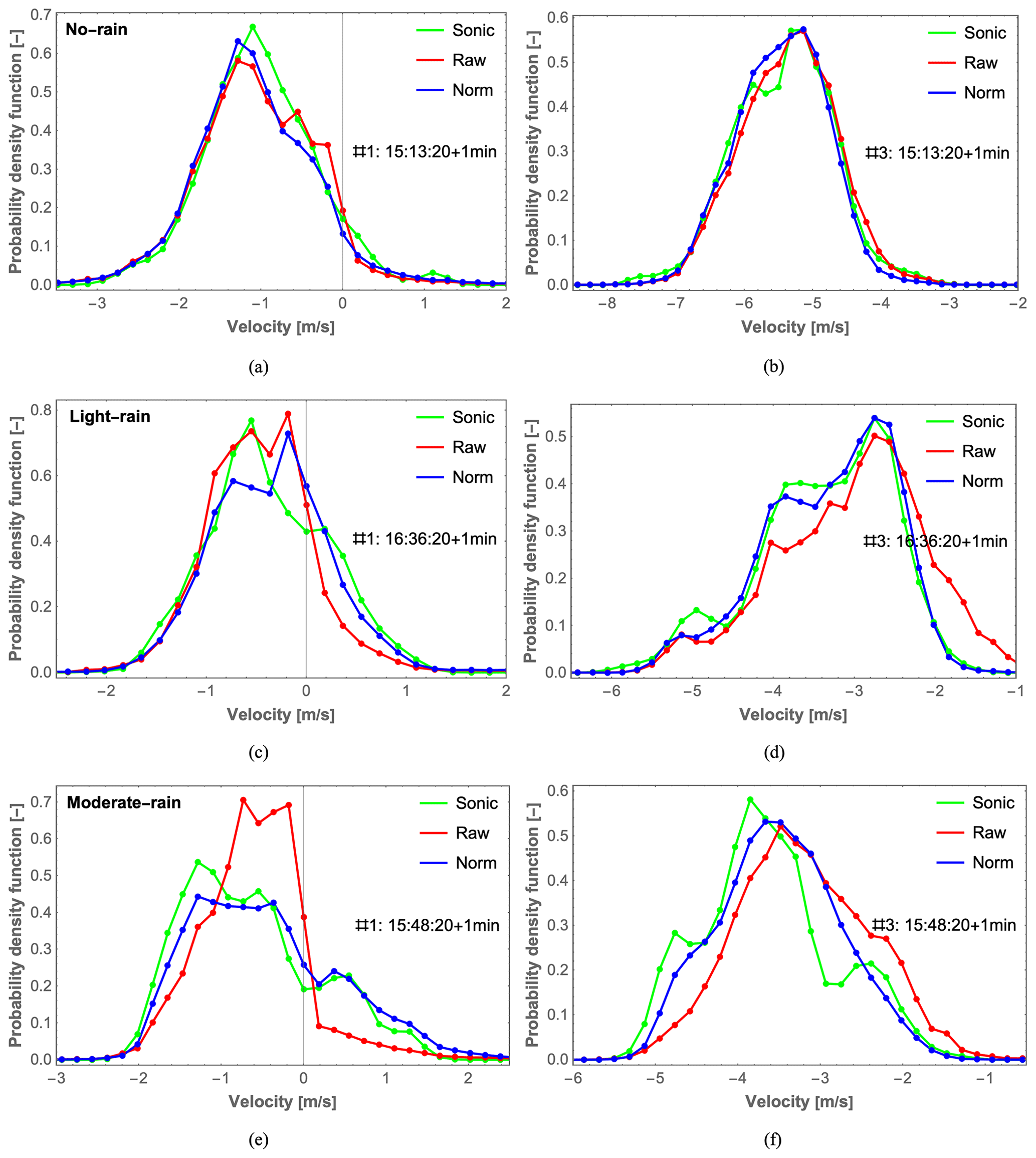
Figure 12 Probability density function (PDF) of the radial wind velocity from 1 min lidar spectra (red and blue) and from 1 min sonic anemometer data (green) obtained during no-rain (a, b), light-rain (c, d), and moderate-rain (e, f) minutes. (a, c, e) Lidar #1. (b, d, f) Lidar #3. The raw and normalized lidar data are marked in red and blue, respectively.

4 Suppression method for the rain bias

4.1 Lidar data processing

Doppler spectra are usually averaged to lower frequencies ranging from 50 Hz to a few hundred Hz. A 50 Hz sampled spectrum can be processed by the following steps (which are shown as the purple path labeled ➁ and ➂ and the dashed purple line in Fig. 8): the spectrum is divided by the background spectrum and its spectral threshold is subtracted to flatten the background noise. Consequently, the line-of-sight velocity is retrieved based on this noise-flattened 50 Hz spectrum after applying Doppler frequency estimation methods (Peña et al., 2015, Chap. 5).

However, from a random 3 kHz spectrum acquired during a minute (15:48 UTC+1) with moderate precipitation, it is obvious that the spectrum sometimes has a very high, narrow peak, as shown in Fig. 9b. This is caused by a raindrop falling through the beam, and the intensity of this should be compared to those in the more commonly occurring spectra where the Doppler signal is caused by aerosols (Fig. 9a). Here, the width of the Doppler spectrum in Fig. 9a is relatively wide because the aerosols within the measurement volume of the lidar have slightly different velocities and the peak value is much lower. In contrast, the spectrum caused by the raindrop is very narrow because of the single velocity of the drop. From the histogram of the maximum values of the spectra obtained during this moderate-rain minute (Fig. 9d), the events with very high backscattering (marked by the red circle) are large raindrops passing through the center line of the laser beam close to the beam waist. These could potentially cause a bias between the radial wind velocities measured by the lidar and the sonic anemometer.

Therefore, based on the above observations, we propose the use of the rain-suppressing normalization method to reduce the influence of rain on wind velocity estimation. The detailed process is indicated by the solid lines and the steps labeled ➀ to ➂ in Fig. 8. These steps are as follows:

• ➀

  Every 3 kHz sampled Doppler spectrum without rain signal suppression (the blue curve labeled “Raw” in Fig. 9a) is divided by the background spectrum (red curve in Fig. 9a) to flatten the noise floor. Then, the noise-flattened 3 kHz sampled spectrum is normalized by its own peak value. Subsequently, every 60 normalized spectra are averaged down to 50 Hz to achieve a better signal-to-noise ratio (Branlard et al., 2013) and ease the comparison with the sonic anemometer.

• ➁

  A spectral threshold (the black line in Fig. 9c) is subtracted from every 50 Hz spectrum, and negative values are zeroed. The spectral threshold is calculated based on the mean value (μ) plus multiple numbers of the standard deviation (σ) of the power spectral density over a wind-signal-free Doppler frequency range.

• ➂

  The median method is used to determine the line-of-sight velocity from the final 50 Hz spectra (Fig. 9c), as it gives smaller biases for weak signals (Angelou et al., 2012a) in comparison to the maximum and centroid methods (Held and Mann, 2018).

In the first step, the background spectrum is calculated as the median power spectral density per frequency of 180 000 Doppler spectra acquired during 1 min. After that, we choose the smaller background for any pair of frequencies $(-f,f)$, which provides the true background noise even if the wind velocity is constant over the minute. However, this procedure will not work if the wind velocity is around zero, since the wind Doppler signal would be present on both sides of the zero frequency bin. Then, a real atmospheric Doppler signal would be included in the background spectrum rather than the real background noise. Therefore, in the case of lidar #1, where the line-of-sight velocity fluctuates around zero (the vertical line at frequency bin 257 corresponding to zero Doppler shift in Fig. 9), a background spectrum is calculated for a period where the line-of-sight speed is away from zero.

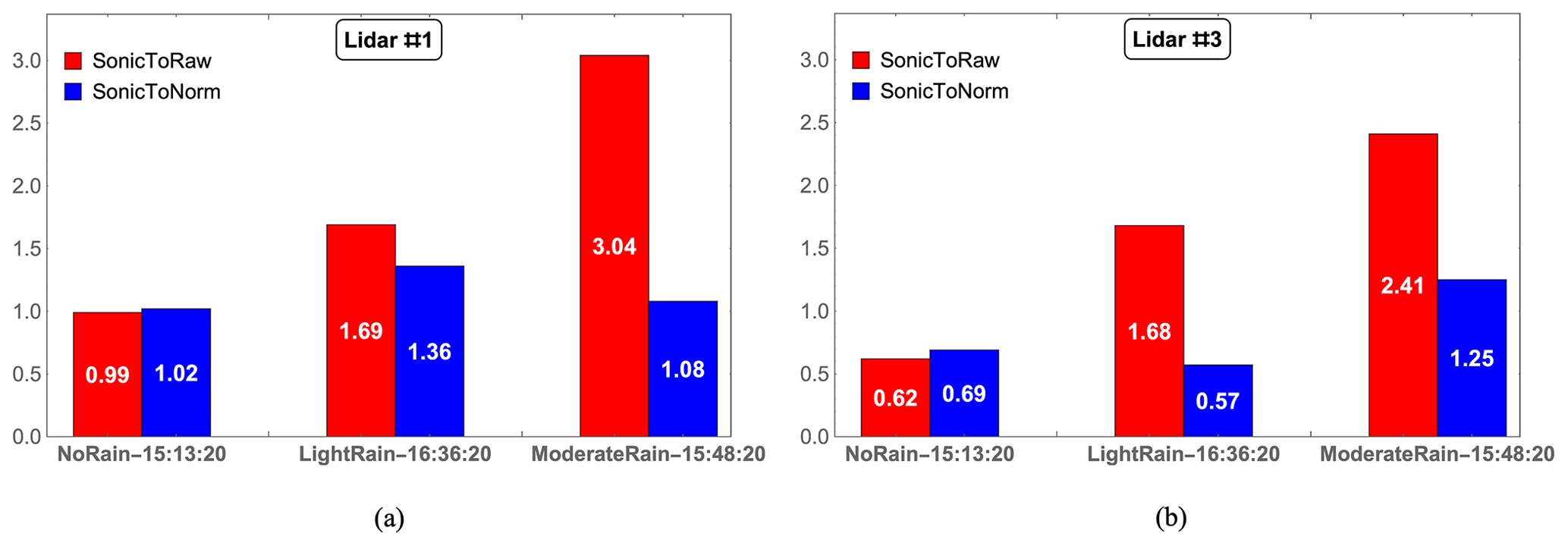
Figure 13 Comparison of the integral value of the absolute difference in PDF between the sonic anemometer and the lidar data with (SonicToNorm) and without (SonicToRaw) rain-suppressing normalization obtained during no-rain, light-rain (I_rain=1 mm h⁻¹), and moderate-rain (I_rain=4 mm h⁻¹) minutes. (a) Lidar #1. (b) Lidar #3.

After obtaining 50 Hz spectra in the third step, it is vital to determine the correct spectral threshold to define the signal caused by the wind in a Doppler spectrum. This is because a spectral threshold that is too high would result in the unexpected removal of the useful Doppler signal and cause a false wind velocity of 0 m s⁻¹, while a spectral threshold that is too low would leave a lot of noise in the spectrum, deteriorating the accuracy of the wind velocity estimation. As concluded in Angelou et al. (2012a), the optimum number of standard deviations to define the threshold is not the same for different data sets. By calculating the velocity difference between lidar data with various spectral thresholds and the sonic anemometer data over a short period of time, a number of 2.5 was chosen for the three lidars in this study.

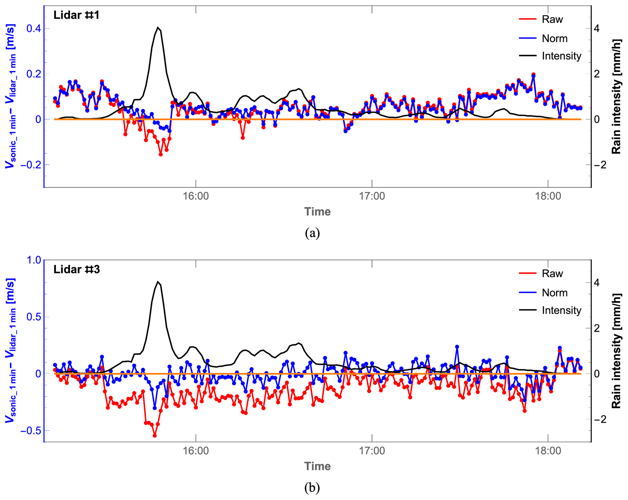
Figure 14 Difference in 1 min averaged wind velocity between lidar and sonic anemometer measurements together with the rain intensity (the solid black curve) from 15:12 to 18:11 UTC+1. (a) Lidar #1 with a probe length of 1.2 m. (b) Lidar #3 with a probe length of 9.8 m. The raw and normalized lidar data are marked in red and blue, respectively.

4.2 Lidar spectra with and without rain-suppressing normalization

It is important to point out that during the measurement time from 15:12 to 18:11 UTC+1, lidar #2 was facing the wind almost all the time, and we speculate that rainwater was covering the entrance window of the lidar telescope despite our attempt to shield the window with a green rain barrel (Fig. 1). The water caused a very weak Doppler spectrum, even during the minute with the highest rain intensity. Therefore, for further analysis and comparison, only the measurement data from lidar #1 and #3 are used.

It is worth noting that the wind direction during the minute with the highest rain intensity (15:48 UTC+1) is from 160^∘ (based on the 10 min averaged sonic anemometer data), and the two lidars' geographic beam directions are 42.6 and 299.3^∘ (Fig. 2). Therefore, the wind is moving away from both lidars' laser beams during this minute, causing a negative line-of-sight velocity. Consequently, the projection of the resultant velocity of raindrops, in the measuring configuration used here, is smaller than that of the horizontal wind speed in the beam direction. In Fig. 10, it is very obvious that after normalization by the spectral peak, the narrow Doppler signal caused by the raindrops (red arrows) is effectively suppressed and the bias between the reference sonic anemometer wind velocity and the wind velocity from each lidar is reduced, as can also be seen in Table 3; for example, the bias decreases from −1.56 to −0.18 m s⁻¹ at 50 Hz for lidar #3. This indicates that normalization by the spectral peak value can help to reduce the influence of the raindrops since the narrow peak closer to the center zero frequency (the solid black line at frequency bin 257) is strongly suppressed.

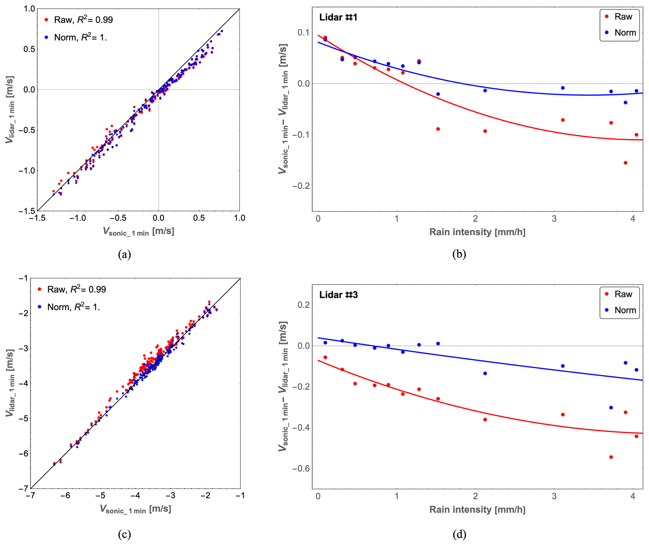
Figure 15 One-minute wind velocity comparison between the lidar and sonic anemometer measurements from 15:12 to 18:11 UTC+1 for lidar #1 (a, b) and lidar #3 (c, d). (a, c) Scatter plot of 1 min wind velocities. (b, d) Averaged bias and the function fitted to it versus the rain intensity. The raw and normalized lidar data are marked in red and blue, respectively.

In the section below, we compare the radial wind velocities detected by lidars and the sonic anemometer at 31 m height in detail in light of the promising results obtained above, i.e., the effective suppression of rain Doppler signals during 1 moderate-rain minute (15:48 UTC+1). The outcomes are elaborated to verify that this rain-suppressing normalization method is applicable under no-rain, light-rain, and moderate-rain conditions.

5 Comparison between lidar and sonic anemometer wind velocities

5.1 Comparison of 50 Hz wind velocities

The reference 50 Hz sonic anemometer data at 31 m height were synchronized with the lidar measurements before the comparison. In Fig. 11, the 50 Hz radial wind velocity time series of the normalized lidar data (blue curve) matches well with the synchronized sonic anemometer data (green curve) during the no-rain, light-rain (I_rain=1 mm h⁻¹), and moderate-rain (I_rain=4 mm h⁻¹) minutes. It is very clear that the fluctuation of the wind velocity caused by the raindrops is effectively suppressed, especially during the moderate-rain period for lidar #1 with a shorter focus distance of 37.2 m (Fig. 11e) or during the rainy period for lidar #3 with a longer focus distance of 103.9 m (Fig. 11d and f). This can also be found from R² values, which indicate that there is less dispersion of the lidar wind velocity after rain-suppressing normalization.

Furthermore, Tables 4 and 5 compare the minute-averaged radial wind velocities of the three data sets (sonic anemometer, original raw lidar data without rain-suppressing normalization, and rain-suppressing normalized lidar data) as well as the bias between the sonic anemometer and lidar estimations. In the case of a small probe length (lidar #1), the bias is only effectively reduced (from −0.15 to −0.04 m s⁻¹) after normalization for the moderate-rain minute, whereas the bias is almost the same after normalization for the no-rain and light-rain minutes. However, the precise wind velocity is obtained after the normalization of lidar #3 data in the presence of light rain and moderate rain, with the bias correspondingly reduced from −0.21 to −0.01 m s⁻¹ and from −0.33 to −0.08 m s⁻¹, respectively. In light of this, it follows that when the probe length is small and it rains more heavily than lightly, rain-suppressing normalization by the spectral peak value can suppress the rain signals effectively. However, when the probe length is larger (up to 10 m), with a broader Lorentzian weighting function, normalization performs very well whenever rain falls (whether light or heavy) because of the sensitivity of the lidar to rain signals.

In addition, the same conclusions can be drawn by comparing the probability density functions (PDFs) calculated for the radial wind velocities estimated based on the 1 min averaged lidar spectra and the 50 Hz sonic anemometer data obtained during 3 min with different rain intensities, as shown in Fig. 12. An improvement following normalization is only observed for lidar #1 (with a smaller probe length) during the moderate-rain period (Fig. 12e), as the calculated integral of the absolute difference in PDF is reduced from 3.04 to 1.08 in Fig. 13. For lidar #3 (with a larger probe length), normalization performs very well not only for the moderate-rain minute in Fig. 12f but also for the light-rain minute in Fig. 12d, reducing the integral of the absolute difference in PDF from 1.68 to 0.57. In a comparison of the integrals of the absolute differences in PDF alone, normalization performs very well during rain periods when the probe length is large or during moderate rain when the probe length is smaller, which is consistent with the conclusions discussed above.

For every minute, the R² of lidar #3 is smaller than that of lidar #1 when comparing the R² values of the original raw lidar data in Fig. 11. We are uncertain about why rain seems to deteriorate the wind signal from lidar #3 more than that from lidar #1. It could have to do with the larger sample volume of #3 or the different elevation angles, but it could also have to do with different numbers of raindrops on the entrance windows of the telescopes. A greater understanding of these sensitivities awaits more experimentation.

5.2 One-minute wind velocity comparison

The bias between the 1 min sonic anemometer wind velocity and the lidar wind velocity, along with the rain intensity, is presented in Fig. 14. From the figure, we can draw similar conclusions to those described previously. In the case of lidar #1 (with a smaller probe length), in Fig. 14a, after normalization with the spectral peak, the large bias of the red curve around the rain intensity peak is effectively reduced from −0.15 to −0.03 m s⁻¹. This is a result of suppressing the low and negative velocities caused by raindrops. For the other minutes, the estimated wind velocity after normalization is almost the same as the raw data, which aligns with the conclusions drawn from the 50 Hz data in Sect. 5.1.

For lidar #3, the improvement in wind velocity estimation achieved by normalization from when it starts to rain at 15:29 until 16:48 UTC+1 is highly effective, as presented in Fig. 14b. Afterward, during some minutes, the wind velocity time series after normalization overlaps with that of the raw lidar data, especially when the rain intensity is below 0.2 mm h⁻¹ after 17:00. For most of the 3 h comparison period, the wind velocity calculated by the raw lidar data is underestimated, as shown in Fig. 14b. This is because of the small projection of the raindrop velocity, which counteracts the aerosol projection and adversely affects the estimated wind velocity. Also, the red curve shows a radial velocity difference of over 0.5 m s⁻¹.

In Fig. 15c, the 1 min lidar wind velocity after rain-suppressing normalization matches well with the sonic anemometer measurement for lidar #3 with a larger probe length, as the normalized lidar data (blue dots) are in a closer agreement with the sonic anemometer measurements compared with the raw lidar data (red dots). For lidar #1 in Fig. 15a, there is no obvious improvement after normalization by the spectral peak. However, the averaged bias in Fig. 15b and d demonstrates the performance of rain-suppressing normalization. It is clearly indicated by the red and blue fitted curves that the suppression is effective not only for lidar #3 when it rains but also for lidar #1 with a short focus distance when the rain intensity is large. Due to the rarity of the passage of raindrops through the laser beam with a condensed probe length, this method does not have a large impact on velocity determinations by lidar #1 during light rain, since there are only 0.05 raindrops in the probe volume in moderate rain. These lead to the same conclusions discussed previously: that rain-suppressing normalization performs well for a large probe length when it rains as well as for a small probe length when it rains more heavily than lightly.

6 Conclusions

In this paper, we have shown an experimental proof-of-concept demonstration of a method to reduce the bias caused by precipitation in continuous-wave Doppler lidar measurements of wind speed. This is accomplished by sampling Doppler spectra faster than most raindrops' beam transit times, which meant sampling at 3 kHz in the current case. Subsequently, the 3 kHz spectra are normalized with their peak values to suppress strong backscatter signals from raindrops before being averaged down to 50 Hz, from which the radial wind velocity is determined.

Results from lidar beams with different elevation angles and focus distances were studied under different rain intensities measured by a disdrometer. The derived wind velocities were compared with a sonic anemometer reference. From the comparison, we found that rain-suppressing normalization has the most significant impact in terms of reducing bias when the probe volume (which grows with the fourth power of the focus distance) is the largest. However, when the probe volume is small (shorter focus distances), the impact of rain is limited. Rain-induced bias also varies according to elevation angle, albeit to a lesser extent. However, the exact nature of these relations remains to be further verified and understood.

The tendency is that the more it rains, the stronger the bias and the more the rain-suppressing normalization reduces the bias. For a moderate rain intensity (we did not have a heavy-rain period in our data), the range of the bias was reduced from the interval 0.1 to 0.4 m s⁻¹ to 0.0 to 0.1 m s⁻¹. The method suggested in this study could also be investigated for use with rain events (containing heavy rain) on several days and also for use with pulsed Doppler lidars, even though their measurement volume is significantly larger than that of continuous-wave lidars. Further investigations could also attempt to retrieve the raindrops' falling velocity as well as the drop-size distribution using fast Doppler spectra.