the Creative Commons Attribution 4.0 License.
the Creative Commons Attribution 4.0 License.
 | 31 Jan 2023
Evaluation of the spectral misalignment on the Earth Clouds, Aerosols and Radiation Explorer/multi-spectral imager cloud product
Takashi Y. Nakajima
Woosub Roh
Masaki Satoh
Kentaroh Suzuki
Takuji Kubota
Mayumi Yoshida
A cloud identification and profiling algorithm is being developed for the multi-spectral imager (MSI), which is one of the four instruments that the Earth Clouds, Aerosols, and Radiation Explorer (EarthCARE) spacecraft will feature. During recent work, we noticed that the MSI response function could shift substantially among some wavelengths (0.67 and 1.65 µm bands) owing to the spectral misalignment (SMILE), in which a shift in the center wavelength appears as a distortion in the spectral image. We evaluated how SMILE affects the cloud retrieval product qualitatively and quantitatively. We chose four detector pixels from bands 1 and 3 with the nadir pixel as the reference to elucidate how the SMILE error affects the cloud optical thickness (τ) and effective cloud droplet radius (re) by simulating the MSI forward radiation with Comprehensive Analysis Program for Cloud Optical Measurement (CAPCOM). We also evaluated the error in simulated scenes from a global cloud system-resolving model and a satellite simulator to measure the effect on actual observation scenes. For typical shallow warm clouds (τ = 8, re = 8 µm), the SMILE error on the cloud retrieval was not significant in most cases (up to 6 % error). For typical deep convective clouds (τ = 8, re = 40 µm), the SMILE error on the cloud retrieval was even less significant in most cases (up to 4 % error). Moreover, our results from two oceanic scenes using the synthetic MSI data agreed well with the forward radiation simulation, indicating that the SMILE error was generally within 10 %. Generally, this negligible impact of the SMILE is true for water surfaces, but it still needs to be investigated further for land surfaces in future works.
- Article
(18680 KB) - Full-text XML
- BibTeX
- EndNote


Clouds and aerosols are key elements of the Earth's water and energy cycle. Atmospheric radiative forcing is affected by cloud alteration due to indirect aerosol effects. Radiative forcing due to cloud–aerosol interactions still cause the greatest uncertainty in estimating changes in the Earth's energy balance (Solomon et al., 2007). Earth Clouds, Aerosols and Radiation Explorer (EarthCARE) is a joint earth observation satellite project between the European Space Agency (ESA) and the Japanese Aerospace Exploration Agency (JAXA; JAXA, 2012) for observing cloud–aerosol interactions (Illingworth et al., 2015). EarthCARE is equipped with four sensors, cloud profiling Radar (CPR), atmospheric lidar, multi-spectral imager, and broadband radiometer. Data products related to clouds, aerosols, and radiation flux are created from single and combined observations from these sensors (Illingworth et al., 2015; Kikuchi et al., 2019).
The MSI (Albiñana et al., 2010) has been developed by the ESA and measures emitted infrared and reflected solar radiances. The MSI has spectral curvature nonlinearity disturbance, which is known as the smile or frown distortion, and is a center wavelength shift that appears as distortions of spectrum images due to spectral misalignment (Fisher et al., 1998; Mouroulis et al., 2000; Yokota et al., 2010; Dadon et al., 2010). In this paper, we use the acronym SMILE, which stands for Spectral MIsaLignmEnt, as a more scientific definition.
The MSI SMILE was reported by the ESA in 2017 (Koopman, 2017). In addition, SMILE has been observed in several previous spaceborne imaging sensors, such as the Hyperion imaging spectrometer (NASA) (Dadon et al., 2010; Green et al., 2003), the Medium Resolution Imaging Spectrometer (MERIS; ESA) (ESA, 2008), and the hyper-spectral imager SUIte (Japanese Ministry of Economy, Trade, and Industry) (Japan Space Systems, 2012). SMILE degrades the spectrum information and reduces classification accuracy, which could cause errors in the cloud retrieval product.
A qualitative and quantitative validation is necessary to evaluate the error caused by SMILE in the MSI cloud retrievals. First, the effect of SMILE on the radiative transfer model used in cloud profiling algorithms was evaluated. To evaluate the error in the actual observation scenes, we also used the Joint Simulator for Satellite Sensors (Joint-Simulator) satellite data simulator, which was developed in the JAXA EarthCARE project (Hashino et al., 2013; Satoh et al., 2016; Roh et al., 2020). The satellite data simulator applies satellite orbit calculations and radiation transmission calculations to the cloud or precipitation and temperature or humidity fields generated by the cloud-resolving models and general circulation models, and it simulates satellite observations, such as radiances and radar reflectivities. Model verification using pseudo-satellite observation data from a satellite data simulator and actual satellite observation data has been proposed (Matsui et al., 2009, 2016; Masunaga et al., 2010; Satoh et al., 2010; Roh and Satoh, 2014, 2018; Roh et al., 2017). In addition, the pre-launch evaluation of the satellite product using a satellite data simulator has also been conducted (Hagihara et al., 2021; Matsui et al., 2013). The advantage of evaluating algorithms using a satellite data simulator is that satellite data and cloud parameters that are completely time–space matched at all pixels can be obtained.
This paper describes the evaluation of errors caused by SMILE in the cloud product for EarthCARE MSI observations, especially the microphysical property retrieval of shallow warm cloud and deep convective cloud. The errors are evaluated using algorithms that calculate the MSI standard product in the JAXA (JAXA, 2021). Furthermore, the MSI cloud algorithm to obtain the cloud microphysical property retrieval data is applied to synthetic MSI data, and the retrieval data are compared with and without SMILE to determine the error. Note that MSI can be used in not only cloud, but also aerosol retrievals; therefore, SMILE could also affect aerosol products, which is beyond the scope of this paper.
Section 2 describes the cloud product algorithm used in this study and the synthetic MSI data, as well as the methods with which we evaluate SMILE. Section 3 presents the results and discussion, and in Sect. 4 we give the conclusions of this study.
EarthCARE MSI has the seven bands for cloud remote sensing shown in Table 1 (Albiñana et al., 2010): two bands in the visible and near infrared region (0.67 and 0.865 µm) for estimating cloud optical thickness (COT, τ); two bands in the short-wave ultra-infrared region (1.65 and 2.21 µm) for estimating cloud particle effective radius (CDR, re); and three bands in the infrared region (8.8, 10.8, and 12.0 µm) for estimating cloud top temperature and identifying cloud phases. The spatial resolution of each band is 500 m and the swath width is only 150 km. In addition, the swath contains 384 pixels (including 24 dummy pixels on both sides), which is asymmetrical to avoid the sun glint area of the ocean during the local afternoon. When EarthCARE MSI is in its descending mode (moving from north to south), the nadir pixel is basically located around the 102nd pixel counted from the west. However, in actual observation, the location of the nadir will fluctuate slightly according to the location of the satellite, and it is a better way to assign the nadir location from the viewing angle than from the pixel number. In this study, we defined the location of the nadir as the 102nd pixel counted from the west, as a constant value. Based on our definition, the pixel distribution of the MSI swath used in this study is shown in Fig. 1. SMILE is largest in bands 1 and 3 (Fig. 2), which means that SMILE could cause errors in both the COT and CDR estimations.
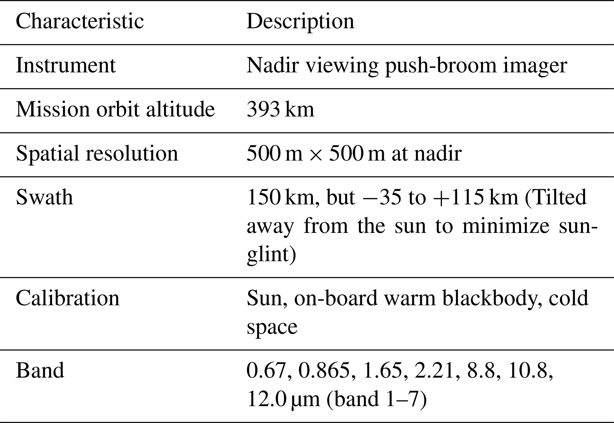
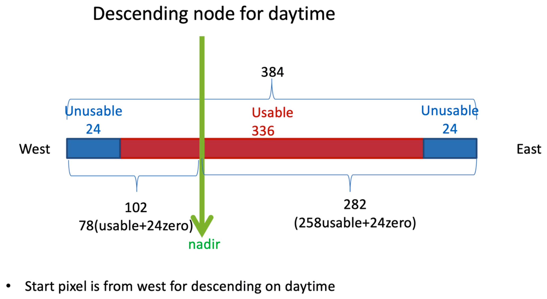
Figure 1Typical pixel distribution of EarthCARE MSI swath used in this study. When EarthCARE MSI is in its descending mode (moving from north to south), the nadir pixel is basically located around the 102nd pixel counted from the west. However, in actual observation, the location of the nadir will fluctuate slightly according to the location of the satellite.
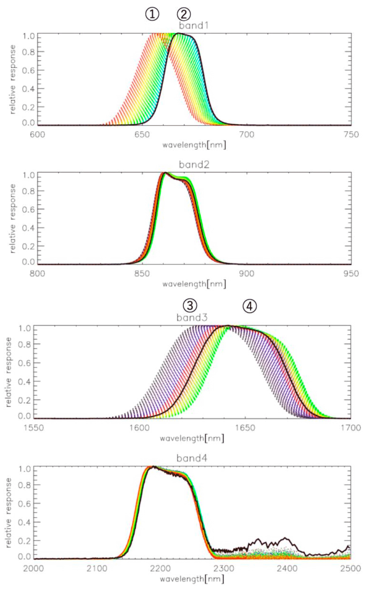
Figure 2Wavelength distribution of relative response function on MSI bands 1 to 4 (Value from flight model). The bold line shows the nadir value. Points 1 to 4 show the positions of Pix_BND1_min, Pix_BND1_max, Pix_BND3_min, and Pix_BND3_max respectively.
2.1 MSI cloud product algorithm
The variables provided by the MSI cloud product contain the cloud flag, cloud phase, COT, CDR, and cloud top temperature. All spatial resolutions are 500 m. The algorithms used to calculate the MSI standard product in the JAXA consist of the cloud flag and cloud phase algorithm (CLAUDIA) and the cloud profiling algorithm (CAPCOM). The CLAUDIA is described in Sect. 2.1.1 and the CAPCOM is described in Sect. 2.1.2.
2.1.1 Cloud flag/cloud phase algorithm
The cloud flag indicates the presence or absence of clouds. The MSI cloud flag algorithm is an optimization of the cloud and aerosol unbiased decision intellectual algorithm (CLAUDIA) reported by Ishida and Nakajima (2009) for the MSI observation bands (JAXA, 2021). CLAUDIA expresses the presence or absence of clouds as a real number from 0 (completely cloudy) to 1 (completely clear-sky), which is called the clear confidence level. During our NICAM and Joint-Simulator data evaluation, we defined two types of cloud: shallow warm cloud (cloud top temperature > 270 K) and deep convective cloud (cloud top temperature < 250 K). We selected two typical scenes for each type of cloud in Sect. 2.2.
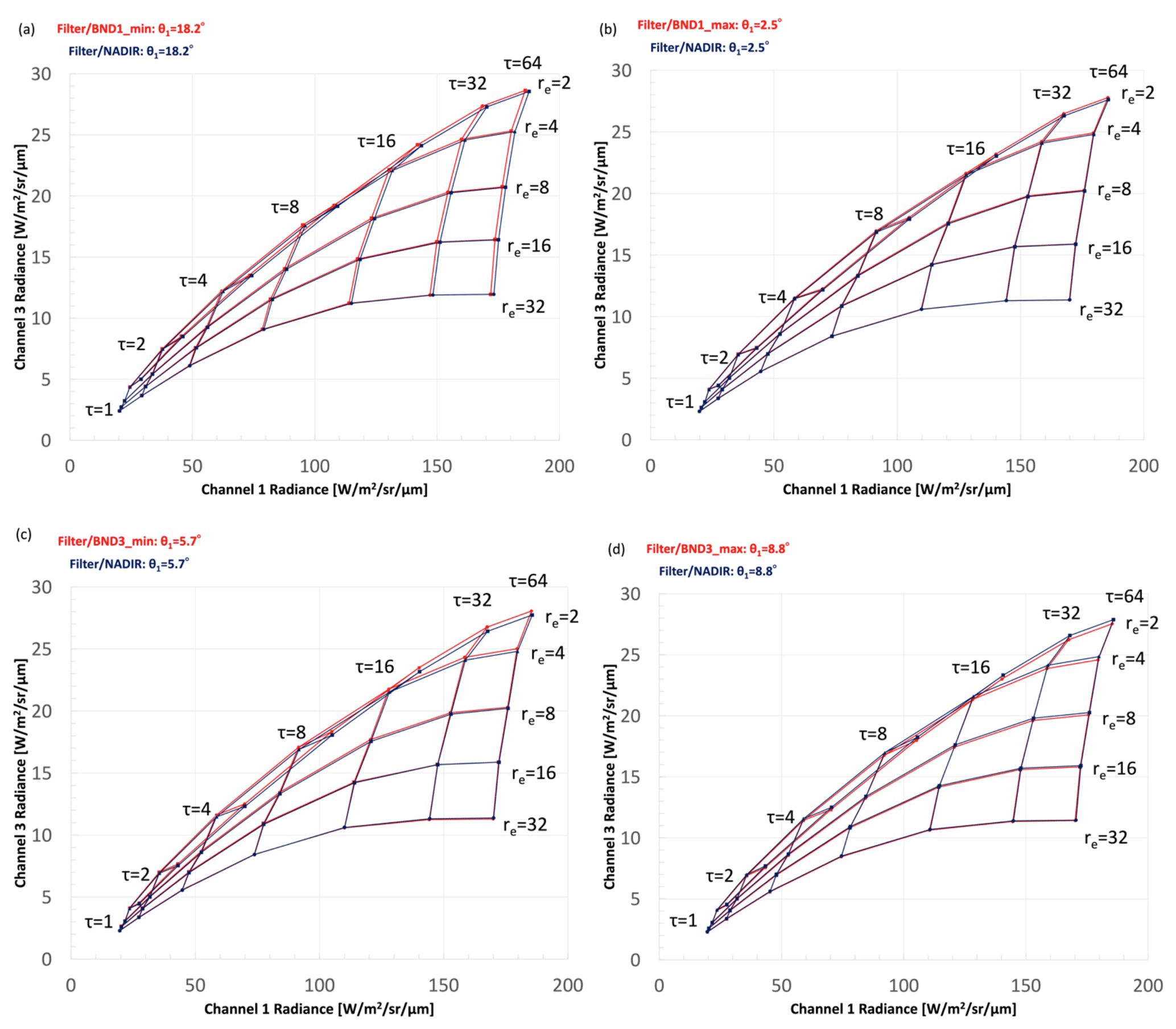
Figure 3Nakajima–King diagrams for shallow warm clouds at (a) pix_BND1_min, (b) pix_BND1_max, (c) pix_BND3_min, and (d) pix_BND3_max for a solar zenith angle of 60∘. The red lines show the results from the response function with SMILE. The black lines show the results from the nadir response function.
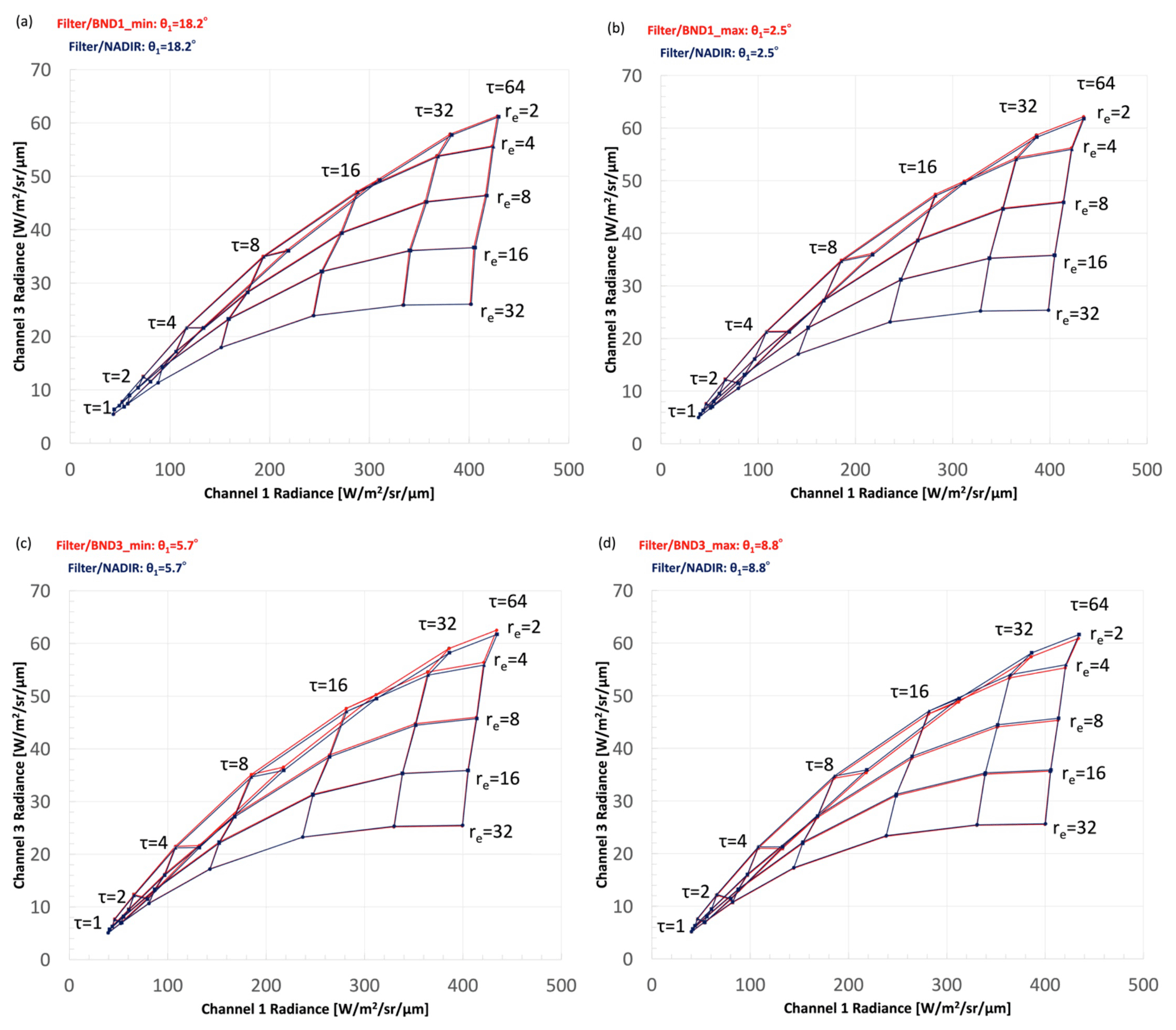
Figure 4Nakajima–King diagrams for shallow warm clouds at (a) pix_BND1_min, (b) pix_BND1_max, (c) pix_BND3_min, and (d) pix_BND3_max for a solar zenith angle of 20∘. The red lines show the results from the response function with SMILE. The black lines show the results from the nadir response function.
2.1.2 Cloud profiling algorithm
The cloud profiling algorithm, which can also be called the cloud microphysical property retrieval algorithm, is an optimization of Comprehensive Analysis Program for Cloud Optical Measurements (CAPCOM) by Nakajima and Nakajima (1995) and Kawamoto et al. (2001) for the observation bands of MSI. CAPCOM-MSI measures COT, CDR, and cloud top temperature from the observed brightness of the visible (0.67 µm), short wavelength infrared (1.65 or 2.21 µm), and thermal infrared (10.8 µm) bands. In CAPCOM, the observed radiance of the 0.67 µm channel contains information about COT, whereas the observed radiance of the 1.65 and 2.21 µm channels contains information about CDR. At 0.67 µm, the imaginary part of the complex refractive index of water is tiny and hardly influenced by the absorption of cloud particles. Therefore, the thicker the cloud optically, the more scattered light travels in the direction of the satellite, and the radiance measured by the satellite increases. In contrast, at wavelengths of 1.65 and 2.21 µm, the imaginary part of the complex refractive index of water is large, so the larger the cloud particle radius, the greater the absorption; thus, the radiance measured by the satellite decreases as the particle size increases. The cloud top altitude and cloud top pressure are estimated from the cloud top temperature using the temperature–altitude or temperature–pressure profile of the objective analysis data. The MSI cloud product provides CDR estimated for bands 3 and 4 (1.65 and 2.21 µm) respectively.
The effective radius of cloud particles, re, is defined as
where r is the particle size and n(r) is the cloud particle number distribution function.
CAPCOM-MSI assumes a lognormal distribution function of the following equation for cloud particle size distribution:
Here, c is a constant, r0 is the mode radius, and σ is the standard deviation of the lognormal distribution (Nakajima et al., 1998). Therefore, the effective radius of cloud particles can be expressed as
CAPCOM-MSI assumes σ = 0.35.
Particle size distribution is considered in the calculation of the COT in CAPCOM-MSI. However, the particle size distribution is used only as a relative value to perceive the frequency dependence of the optical thickness. Therefore, the COT is not directly calculated from the particle size distribution.

Figure 5Nakajima–King diagrams for deep convective clouds at (a) pix_BND1_min, (b) pix_BND1_max, (c) pix_BND3_min, and (d) pix_BND3_max for a solar zenith angle of 60∘. The red lines show the results from the response function with SMILE. The black lines show the results from the nadir response function.
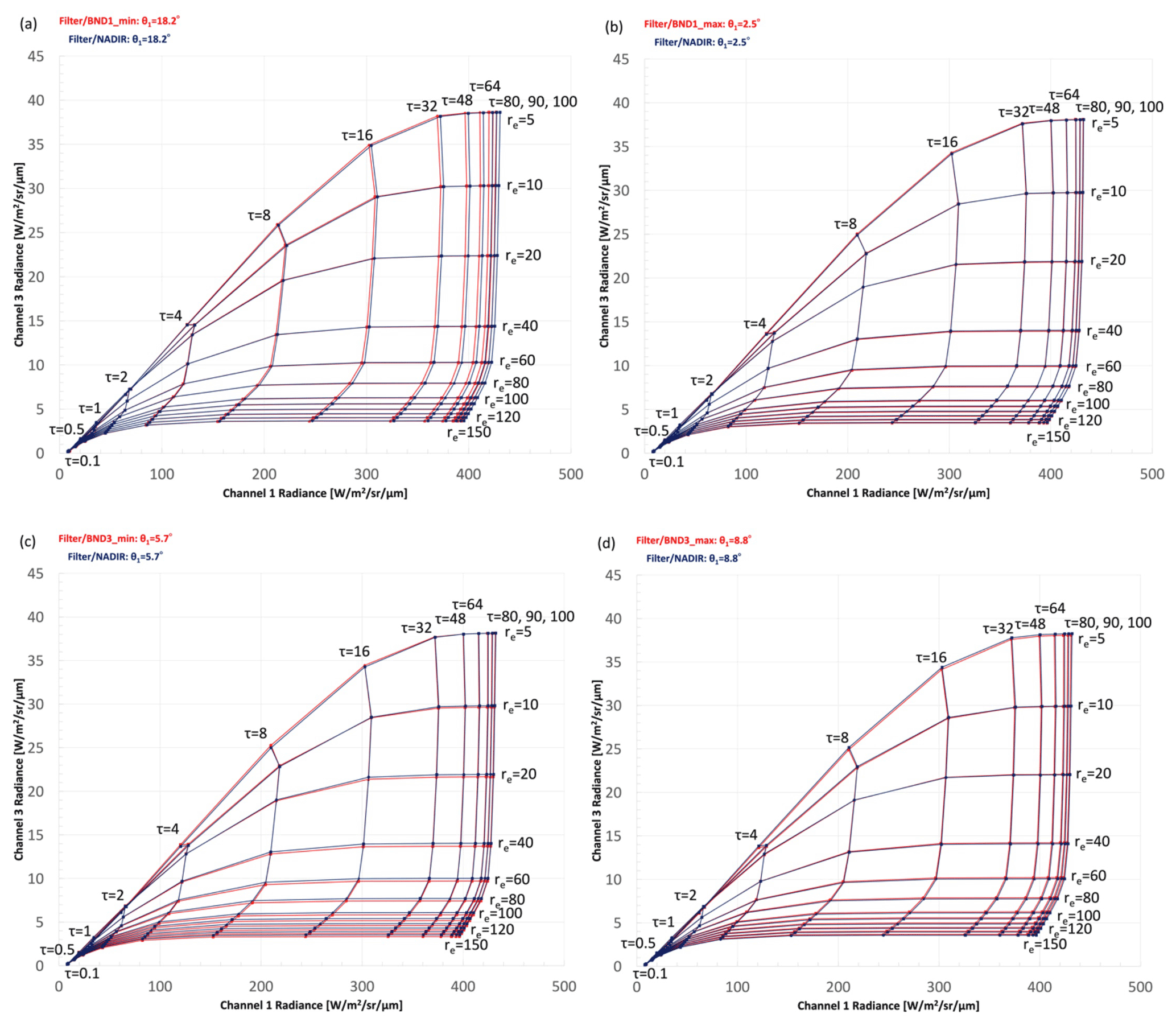
Figure 6Nakajima–King diagrams for deep convective clouds at (a) pix_BND1_min, (b) pix_BND1_max, (c) pix_BND3_min, and (d) pix_BND3_max for a solar zenith angle of 20∘. The red lines show the results from the response function with SMILE. The black lines show the results from the nadir response function.
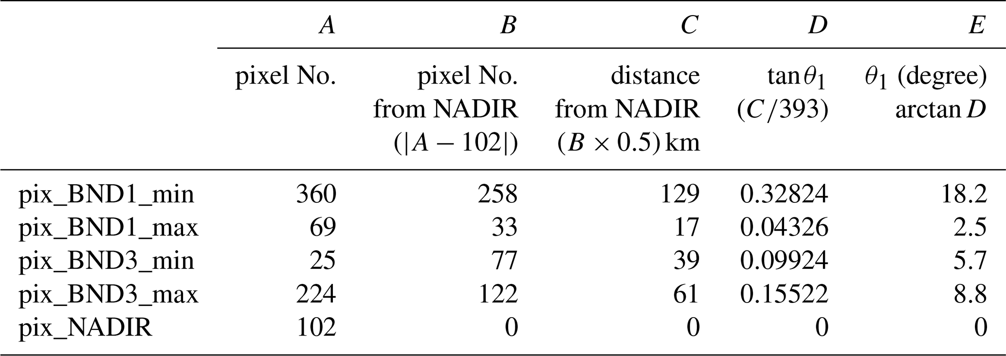
The radiation transfer calculation of CAPCOM-MSI is accelerated by using the look-up table created by the one-dimensional radiation transfer code RSTAR (Nakajima and Tanaka, 1986, 1988; Stamnes et al., 1988). Generally, the response function used for radiation transfer calculation in CAPCOM-MSI is based on the measured value at the nadir location, which was provided by the ESA. The bold line in Fig. 2 shows the nadir reference function. We also selected the following four pixels: pix_BND1_min, which gives the response function of the leftmost (shortest wave) in band 1; pix_BND1_max, which gives the response function of the rightmost (longest wave) in band 1; pix_BND3_min, which gives the response function of the leftmost (shortest wave) in band 3; and pix_BND3_max, which gives the response function of the rightmost (longest wave) in band 3. We obtained the response functions at these pixels to evaluate the effects of shifts in the response functions of bands 1 and 3 on the retrieval estimates of cloud microphysical properties. For reference, we also used pix_NADIR, which gives the response function at the nadir pixel. The positions of four selected pixels are shown in Fig. 2 as points 1 to 4. The information for all five pixels is shown in Table 2. We set the solar zenith angle (θ) as 20 or 60∘ when simulating the radiance.
Table 2Pixels selected for SMILE evaluation. The pixel number of the nadir is 102, θ1 is the satellite zenith angle.
To evaluate the error caused by SMILE in the radiation transfer, we used Nakajima–King diagrams. Nakajima–King diagrams were developed for estimating COT and CDR using two wavelength observations in the visible light (e.g., band 1 of MSI) and near-infrared light (e.g., band 3 of MSI) regions (Nakajima and King, 1990; Nakajima et al., 1991). These diagrams are used as the basis of remote sensing of cloud characteristics from visible and near-infrared light observations.
In the EarthCARE MSI project, cloud characteristic products are divided into standard (water cloud) and research (ice cloud) products. This is because the calculations for water clouds are simpler because the particle shape is roughly spherical, and it is classified as a standard product because it has been analyzed in many projects. In contrast, ice clouds usually have a much greater variety of cloud particle shapes and are classified as research products because they include research elements. Previous research on the EarthCARE MSI analysis proposed the use of electromagnetic wave scattering solutions using Voronoi-shaped particles (Letu et al., 2016, 2019). Voronoi-shaped particles are also used in the EarthCARE MSI algorithm for the ice cloud product.
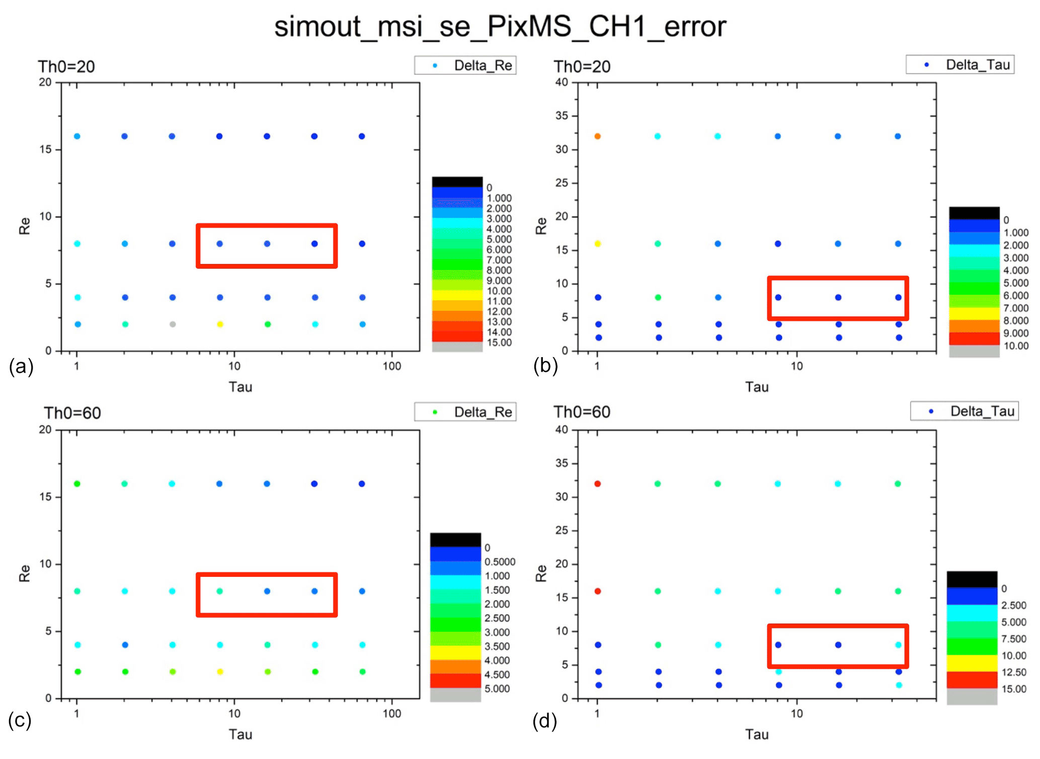
Figure 7Error distributions of COT and CDR from the Nakajima–King diagram for shallow warm clouds at pix_BND1_min. (a) Distribution of Δre for a solar zenith angle of 20∘. (b) Distribution of Δτ for a solar zenith angle of 20∘. (c) Distribution of Δre for a solar zenith angle of 60∘. (d) Distribution of Δτ for a solar zenith angle of 60∘. The red frames indicate the presence of typical shallow warm cloud. COT = 8 or 32, CDR = 8 µm.
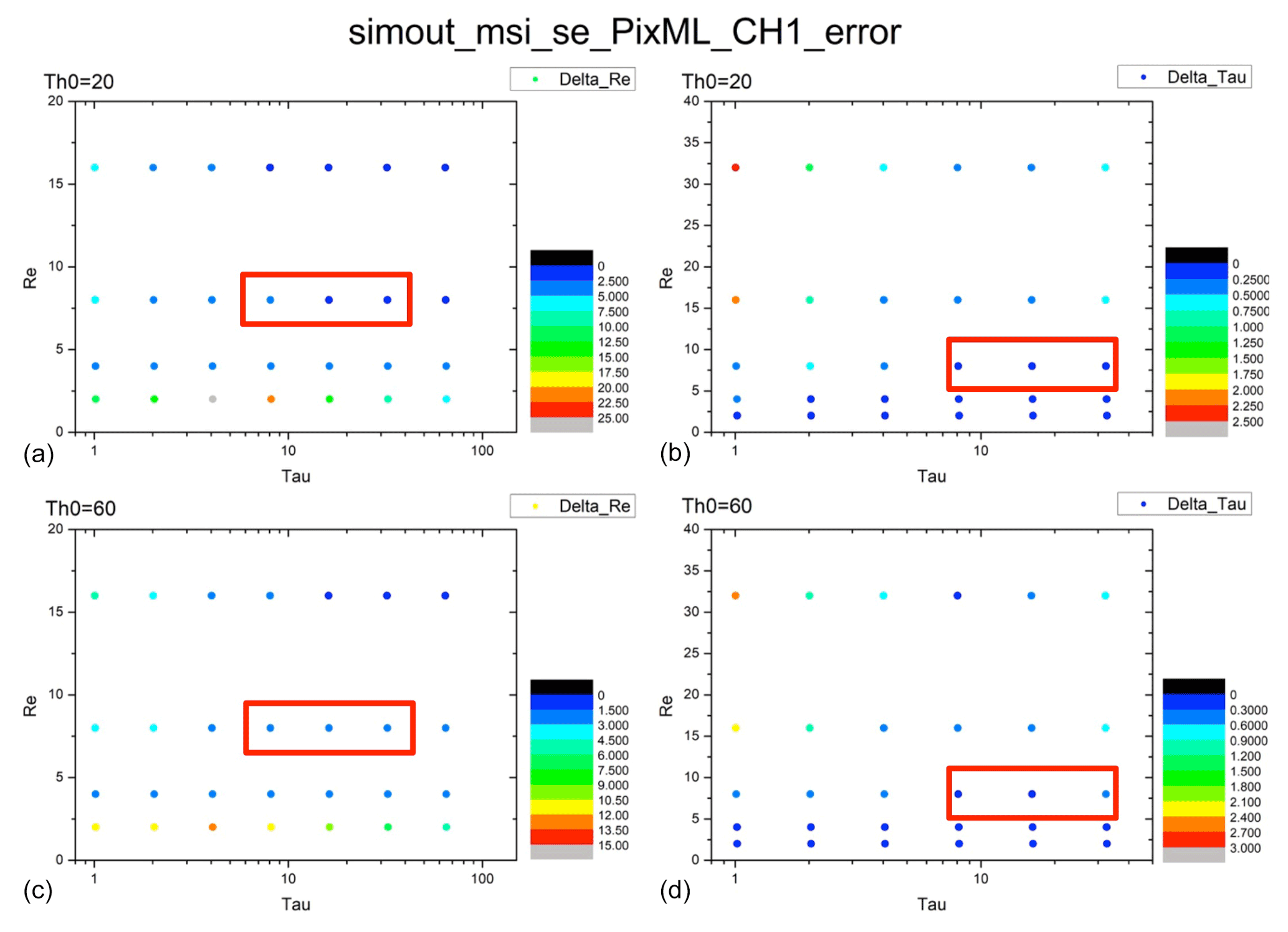
Figure 8Error distributions of COT and CDR from the Nakajima–King diagram for shallow warm clouds at pix_BND1_max. (a) Distribution of Δre for a solar zenith angle of 20∘. (b) Distribution of Δτ for a solar zenith angle of 20∘. (c) Distribution of Δre for a solar zenith angle of 60∘. (d) Distribution of Δτ for a solar zenith angle of 60∘. The red frames show the presence of typical shallow warm cloud. COT = 8 or 32, CDR = 8 µm.
In this study, the combination of COT and CDR to plot Nakajima–King diagrams is defined as follows. For shallow warm clouds, COT (τ) was 1, 2, 4, 8, 16, 32, 48, and 64, and CDR was 2, 4, 8, 16, and 32 µm. For deep convective clouds (Voronoi-shaped particles), COT (τ) was 0.1, 0.5, 1, 2, 4, 8, 16, 32, 48, 64, 80, 90, and 100, and CDR was 5, 10, 20, 40, 60, 80, 100, 110, 120, 130, 140, and 150 µm. We selected the following two combinations of COT and CDR as typical shallow warm clouds and deep convective clouds: for shallow warm clouds, COT was 8 or 32 and CDR was 8 µm; for deep convective clouds, COT was 8 or 32 and CDR was 40 µm.
To evaluate the error of COT and CDR quantitatively, we obtained the first derivation of radiance, ΔL, with respect to COT or CDR from the Nakajima–King diagram as and , and then we obtained the reciprocals as and respectively, and multiplied them by the radiance deviation ΔL between the two response functions (at one of four selected pixels, and on the nadir location) to get the COT and CDR estimation errors, Δτ and Δre respectively. The results for the error distributions are discussed in Sect. 3.2.
The accuracy requirements for COT and CDR are defined in terms of cloud water content. The liquid water path, LWP, of cloud is calculated from the retrieved COT (τc) and the effective radius of cloud particles as
where ρ is the density of liquid water.
2.2 Synthetic MSI data
The synthetic MSI L1 data for MSI cloud product algorithm were created by the Joint-Simulator (Hashino et al., 2013; Satoh et al., 2016), and input 3.5 km-mesh global atmospheric simulation data. The data were calculated by a global storm-resolving atmospheric model, the Nonhydrostatic Icosahedral Atmospheric Model (NICAM) (Tomita and Satoh, 2004; Satoh et al., 2008, 2014). Clouds and precipitation in NICAM are computed by the cloud microphysics scheme, the NICAM Single Moment Water 6 (NSW6) (Tomita, 2008; Satoh et al., 2014). See previous works (Hashino et al., 2013; Yamada et al., 2016; Nasuno et al., 2016) for details of the NICAM data. The advantage of the current NICAM simulation data is that they have already been analyzed in several papers (Hashino et al., 2013, 2016; Matsui et al., 2016; Yamada et al., 2016; Nasuno et al., 2016; Roh et al., 2017; Kubota et al., 2020). The NICAM data were also used in the EarthCARE CPR Doppler simulation (Hagihara et al., 2021). This enables total understanding of the simulation data (including biases) and appropriate interpretations of the results in developing the satellite data algorithms. The simulation started from 00:00Z 15 June 2008, and the synthetic MSI L1 data are calculated by using the NICAM data on 00:00Z 19 June 2008. We selected two oceanic scenes for typical shallow warm clouds and two for typical deep convective clouds, each with 384 pixels in the direction of the swath and 896 pixels in the direction of the track. The geographical location of the shallow warm cloud scenes was 177–178∘ W, 22–25∘ S, and that for the deep convective cloud scenes was 175–176∘ W, 13–16∘ S.
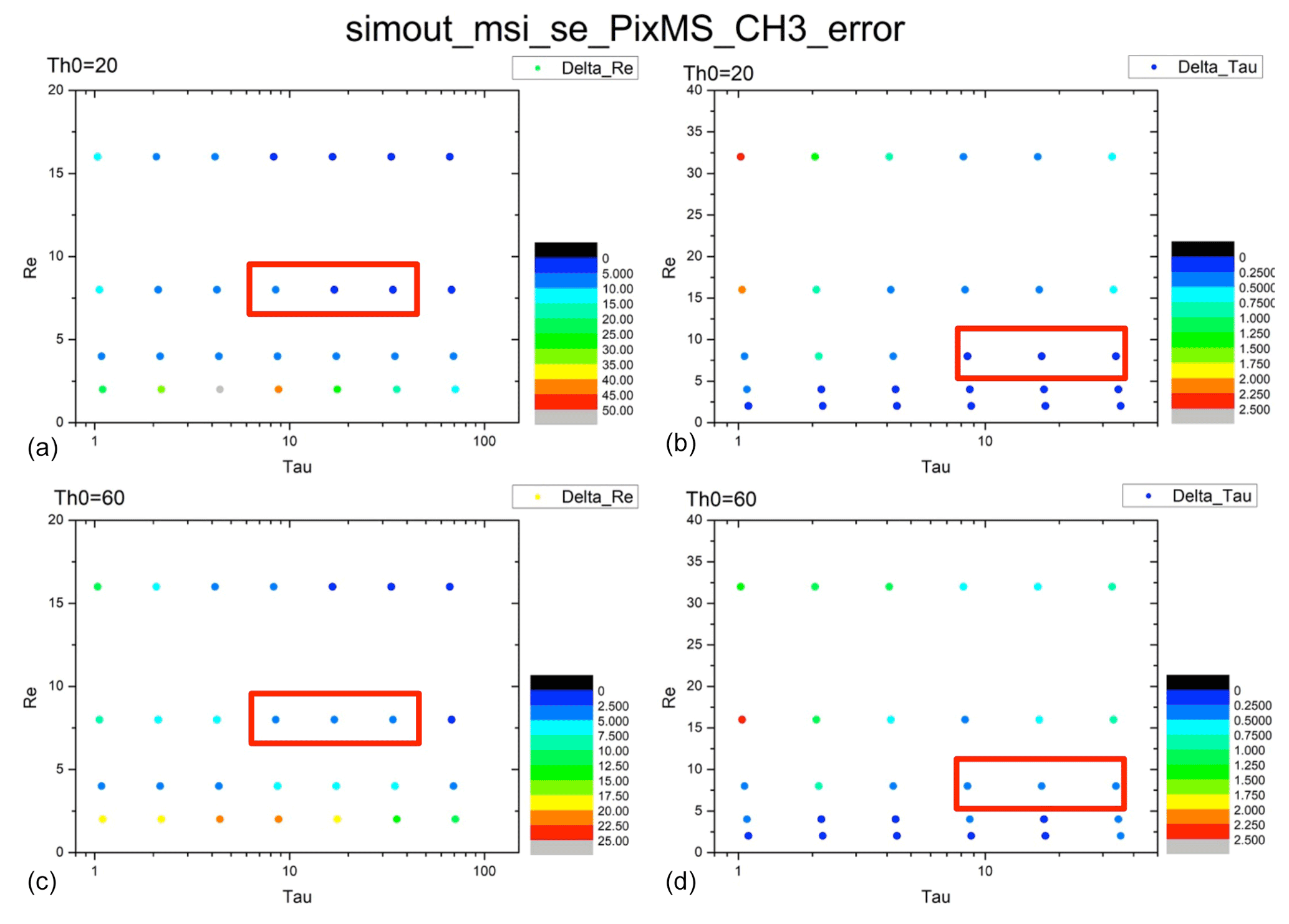
Figure 9Error distributions of COT and CDR from the Nakajima–King diagram for shallow warm clouds at pix_BND3_min. (a) Distribution of Δre for a solar zenith angle of 20∘. (b) Distribution of Δτ for a solar zenith angle of 20∘. (c) Distribution of Δre for a solar zenith angle of 60∘. (d) Distribution of Δτ for a solar zenith angle of 60∘. The red frames show the presence of typical shallow warm cloud. COT = 8 or 32, CDR = 8 µm.
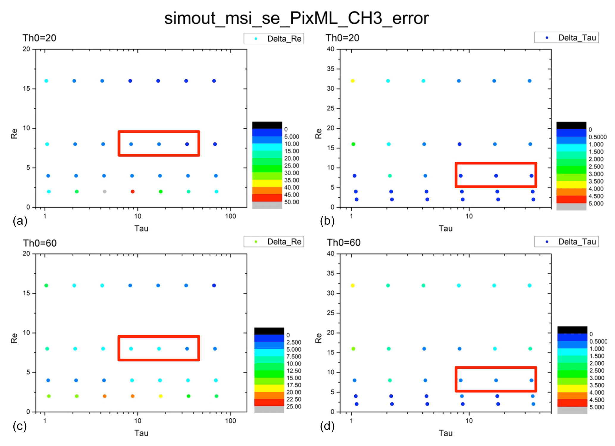
Figure 10Error distributions of COT and CDR from the Nakajima–King diagram for shallow warm clouds at pix_BND3_max. (a) Distribution of Δre for a solar zenith angle of 20∘. (b) Distribution of Δτ for a solar zenith angle of 20∘. (c) Distribution of Δre for a solar zenith angle of 60∘. (d) Distribution of Δτ for a solar zenith angle of 60∘. The red frames show the presence of typical shallow warm clouds. COT = 8 or 32, CDR = 8 µm.
There are several sensor simulators in the Joint-Simulator. The R System for Transfer of Atmospheric Radiation-7 (RSTAR7) (Nakajima and Tanaka, 1986, 1988; Nakajima et al., 2003) was used to simulate radiances and brightness temperatures of MSI in the Joint-Simulator. The size distributions for cloud ice and cloud water are not defined by the cloud microphysics scheme in NICAM (NSW6). Therefore, effective radii of 40 and 8 µm were used for the cloud ice and cloud water in the Joint-Simulator respectively. Single scatterings of hydrometeors as spherical shapes were calculated using the Mie theory in the Joint-Simulator. We interpolated the response function using 60 bins for each channel. SMILE was considered using response functions depending on the pixel number from ESA (Fig. 2). MSI data were generated using the fixed response function at the nadir location as the control data. By applying the MSI algorithm to the nadir and SMILE sets of simulated radiance data, we compared the two sets of cloud retrieval product and evaluated the error caused by SMILE.
2.3 Evaluation criteria for SMILE error
As our evaluation criteria for SMILE error, we performed the following analytical estimation of shortwave radiation (Fsw) due to re change under the assumed constant cloud water content, W.
First, we have the formulation of Fsw,
where S0 is solar constant (approximately 1370 W m−2), n is cloud cover, Δα is the change of cloud albedo.
As the optical thickness of the gas-only atmosphere is approximately 0.2, the changes in global mean shortwave radiation according to Δα can be expressed as Eq. (5).
From Eq. (5) we get the relationship between the change of albedo (Δα) and COT (Δτ),
Meanwhile,
Equation (9) is a theoretical relationship that was used in previous works (Brenguier et al., 2011), where :
assuming that W is constant (ΔW = 0), and
and according to Eqs. (5), (6), and (12), we assumed that global mean optical thickness τ = 7 and g = 0.85; thus, from Eq. (6) we get α=0.51.
Then, Eq. (5) becomes
According to Eq. (13), under the global mean distribution, if CDR decreased by 10 %, then Fsw would decrease by about 4.2 W m−2.
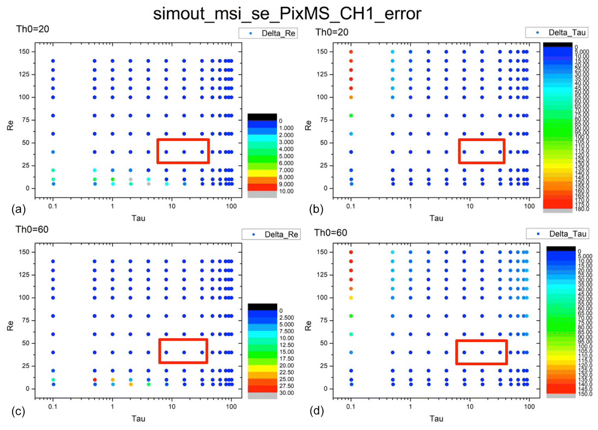
Figure 11Error distributions of COT and CDR from the Nakajima–King diagram for deep convective clouds at pix_BND1_min. (a) Distribution of Δre for a solar zenith angle of 20∘. (b) Distribution of Δτ for a solar zenith angle of 20∘. (c) Distribution of Δre for a solar zenith angle of 60∘. (d) Distribution of Δτ for a solar zenith angle of 60∘. The red frames show the presence of typical deep convective clouds. COT = 8 or 32, CDR = 40 µm.
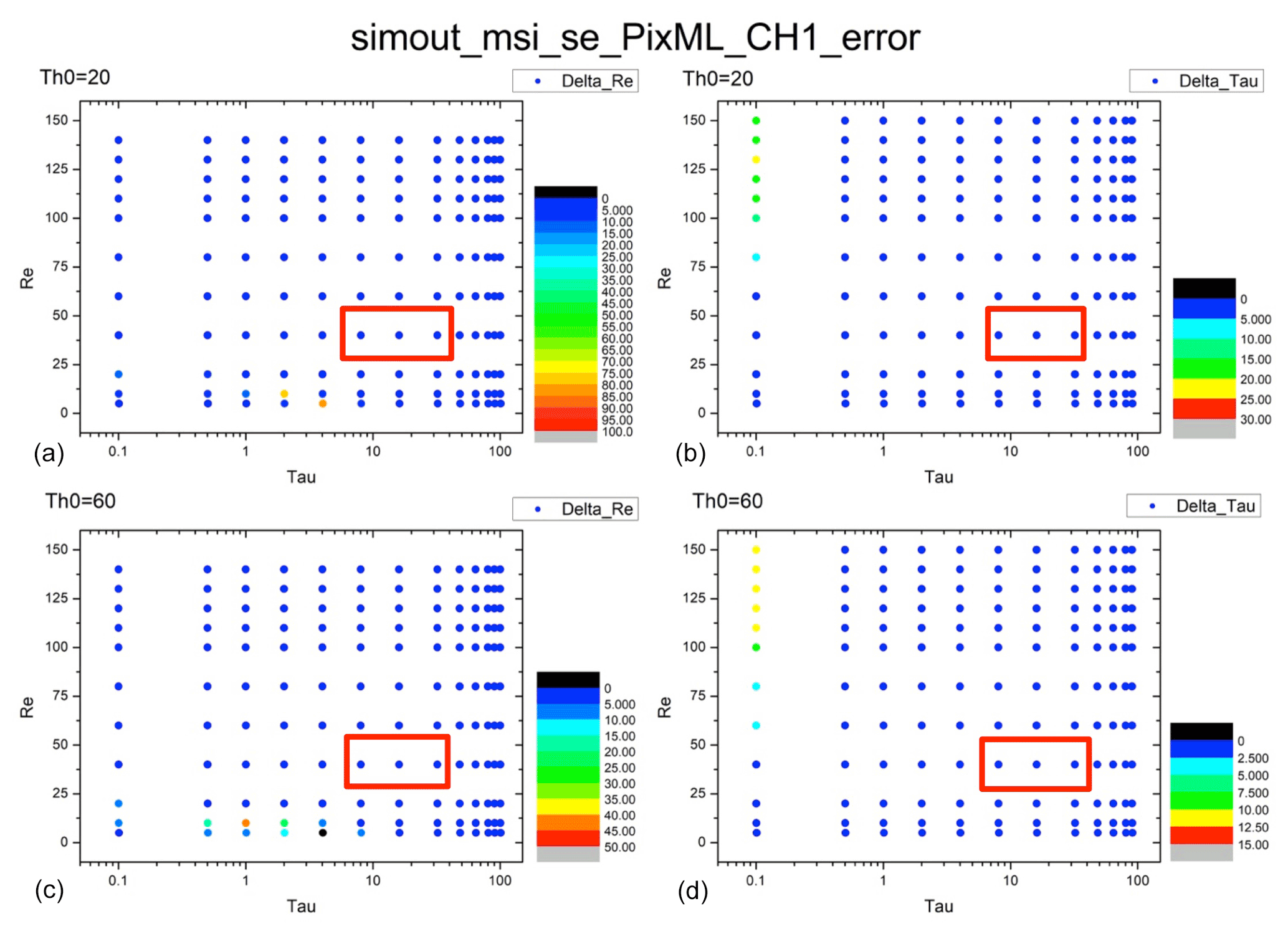
Figure 12Error distributions of COT and CDR from the Nakajima–King diagram for deep convective clouds at pix_BND1_max. (a) Distribution of Δre for a solar zenith angle of 20∘. (b) Distribution of Δτ for a solar zenith angle of 20∘. (c) Distribution of Δre for a solar zenith angle of 60∘. (d) Distribution of Δτ for a solar zenith angle of 60∘. The red frames show the presence of typical deep convective clouds. COT = 8 or 32, CDR = 40 µm.
When W is constant (ΔW = 0), we know that
and we can rewrite Eq. (13) as
Similar to Eq. (13), under the global mean distribution, if COT increased by 10 %, then Fsw would also decrease by about 4.2 W m−2.
An error of this size or larger would be non-negligible in the cloud profiling algorithm of EarthCARE MSI. Therefore, we focused on every Δτ and Δre result to ensure that in most cases, the error caused by SMILE did not exceed this value.
3.1 SMILE in radiation transfer simulation (Nakajima–King diagrams)
The Nakajima–King diagrams for shallow warm clouds are shown in Fig. 3 (solar zenith angle θ0 = 60∘) and Fig. 4 (θ0 = 20∘). The red lines show the results obtained using the response function with SMILE in Pix_BND1_min, Pix_BND1_max, Pix_BND3_min, and Pix_BND3_max. The black lines show the results obtained using the response function located at the nadir pixel, which is not affected by SMILE. The satellite zenith angle for each pixel is shown in Table 2. In pixels in band 1 (Figs. 3a, b and 4a, b), the COT error (Δτ) is much larger than the CDR error (Δre), whereas the opposite is observed in pixels in band 3 (Figs. 3c, d and 4c, d). This is because the observed radiance of the 0.67 µm channel mainly contains information about COT, whereas the observed radiance of the 1.65 and 2.21 µm channels contains information about CDR, as we mentioned in Sect. 2.1.2.
The Nakajima–King diagrams for deep convective clouds are shown in Fig. 5 (θ = 60∘) and Fig. 6 (θ = 20∘). The same trends for Δτ and Δre as for shallow warm clouds are seen for deep convective clouds. Although we had wide ranges for COT (up to 100) and CDR (up to 150 µm) in our simulation, these extreme values do not exist in general in ice cloud research products because such large COT and CDR values usually occur for no ice clouds.
Based on the Nakajima–King diagrams, we calculated Δτ and Δre for typical shallow warm cloud and deep convective cloud cases and the results are shown in Tables 3 and 4. The trends in Δτ and Δre, which we mentioned in Sect. 2.1.2, were also observed here, but Δτ and Δre did not exceed our 10 % evaluation criteria.
Table 3Errors of COT and CDR for typical shallow warm cloud (τ = 8 or 32, re = 8 µm).

θ0 = solar zenith angle, τ = optical thickness, re = effective radius of cloud droplet.
Table 4Errors of COT and CDR for typical deep convective cloud (τ = 8 or 32, re = 40 µm).
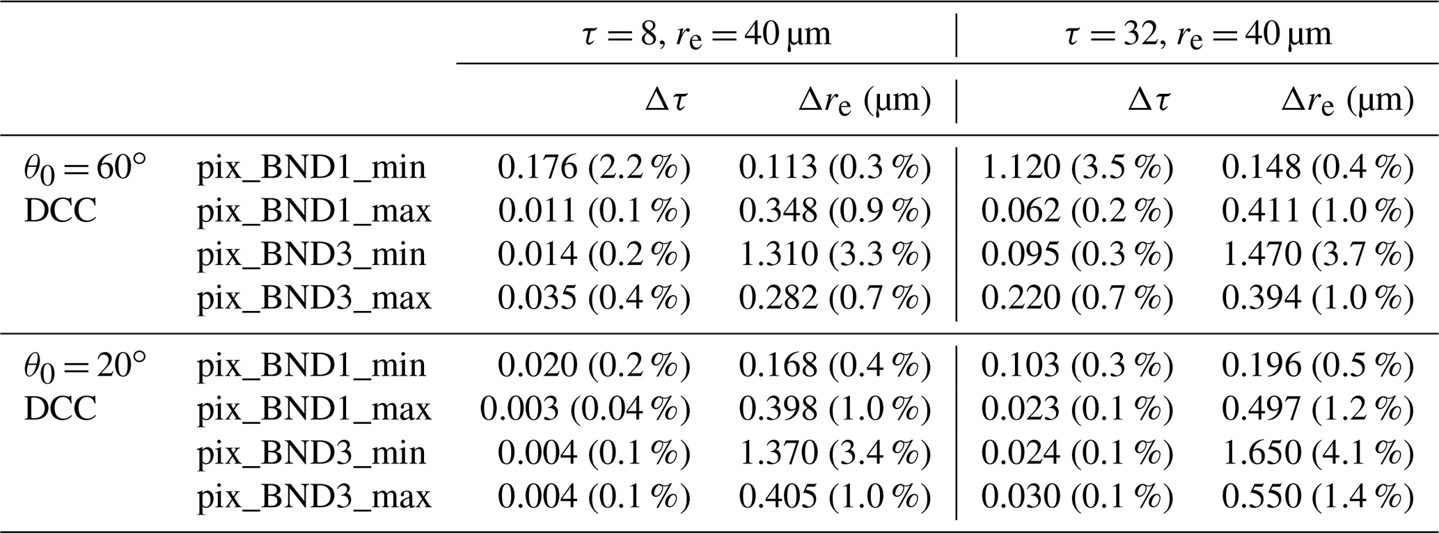
θ0 = solar zenith angle, τ = optical thickness, re = effective radius of cloud droplet.
3.2 Error distribution in radiation transfer
The error distributions for every combination of COT and CDR mentioned in Sect. 2.1.2 are shown in Figs. 7–10 for the shallow warm clouds and Figs. 11–14 for the deep convective clouds at Pix_BND1_min, Pix_BND1_max, Pix_BND3_min, and Pix_BND3_max. The top two panels in every figure show the results for a solar zenith angle of 20∘, and the bottom two panels show the results for a solar zenith angle of 60∘. The left two panels in every figure show the distributions of Δre, and the right two panels show the distributions of Δτ. The red frames show the position of typical shallow warm clouds (COT = 8 or 32, CDR = 8 µm) or deep convective clouds (COT = 8 or 32, CDR = 40 µm) in each panel.
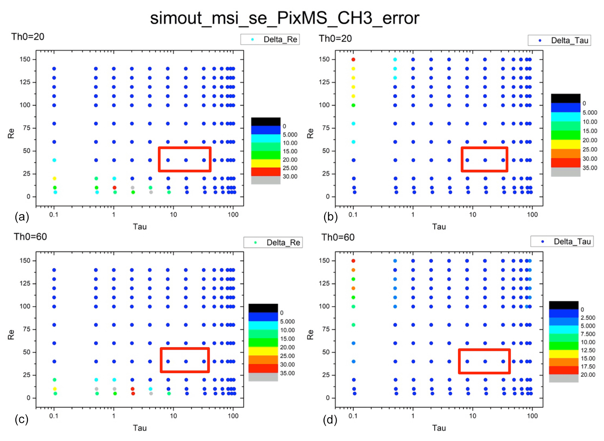
Figure 13Error distribution of COT and CDR from Nakajima–King diagram for deep convective clouds, at pix_BND3_min. (a) Distribution of Δre for a solar zenith angle of 20∘. (b) Distribution of Δτ for a solar zenith angle of 20∘. (c) Distribution of Δre for a solar zenith angle of 60∘. (d) Distribution of Δτ for a solar zenith angle of 60∘. The red frames show the presence of typical deep convective clouds. COT = 8 or 32, CDR = 40 µm.
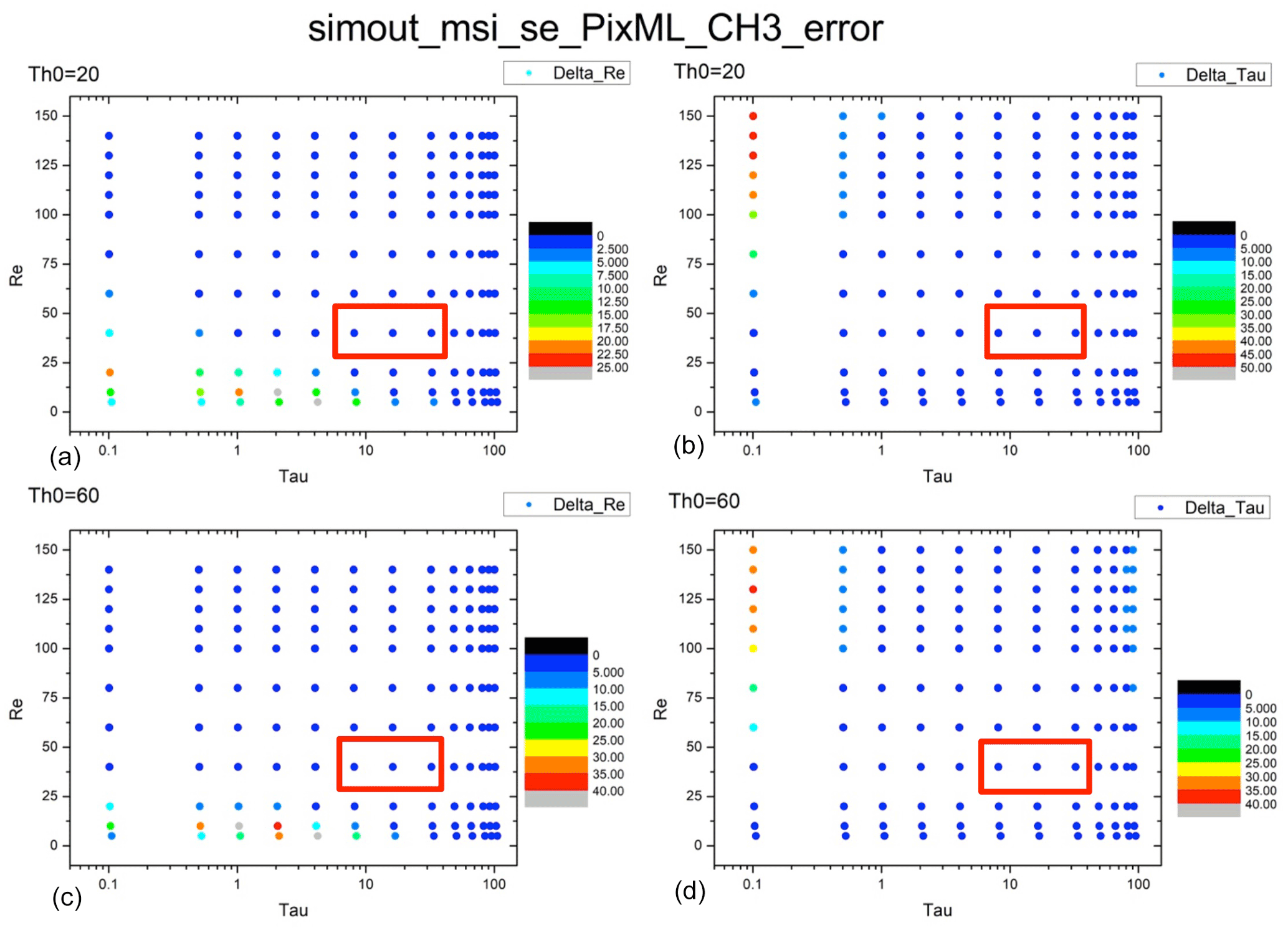
Figure 14Error distributions of COT and CDR from the Nakajima–King diagram for deep convective clouds at pix_BND3_max. (a) Distribution of Δre for a solar zenith angle of 20∘. (b) Distribution of Δτ for a solar zenith angle of 20∘. (c) Distribution of Δre for a solar zenith angle of 60∘. (d) Distribution of Δτ for a solar zenith angle of 60∘. The red frames show the presence of typical deep convective clouds. COT = 8 or 32, CDR = 40 µm.
According to all 32 panels in Figs. 7–14, none of the Δτ and Δre values of typical clouds exceed our 10 % evaluation criteria, which are also shown in Tables 3 and 4. Δτ and Δre are high when low COT (τ = 1 or 0.1) and CDR (re = 2 or 5 µm) values are used in the calculation, as shown by the red-orange dots in the bottom-left part of some Δre panels and in the top-left part of some Δτ panels. Especially in Fig. 11 (Pix_BND1_min for deep convective cloud case), extreme values of Δτ can even exceed 100 %. This is because the derivative of radiance, ΔL, is much larger during the radiation transfer simulation with COT and CDR values that are too low (COT < 1 for both clouds, CDR < 3 µm for shallow warm cloud, and CDR < 10 µm for deep convective cloud), and generally very low COT and CDR values are rare for cloud properties. Thus, none of these high error results has a definitive meaning and is negligible in SMILE error evaluation. Similarly, points with very high CDR (> 100 µm) and very low COT (0.1) in deep convective cloud panels are also unrealistic for cloud properties, which means that these cases are also negligible during our evaluation, regardless of how large the error is.
3.3 Error evaluation in NICAM/Joint-Simulator data
The results of the NICAM and Joint-Simulator simulation data are shown in Fig. 15 (shallow warm clouds) and Fig. 16 (deep convective clouds). Figures 15a and 16a show the radiance at 0.659 µm (band 1 of MSI) and brightness temperature at 10.8 µm (band 6 of MSI) respectively. These two panels show the approximate location of target clouds by marking areas with relatively high radiance (yellow-red areas in Fig. 15a) and relatively low brightness temperature (blue areas in Fig. 16a) respectively.
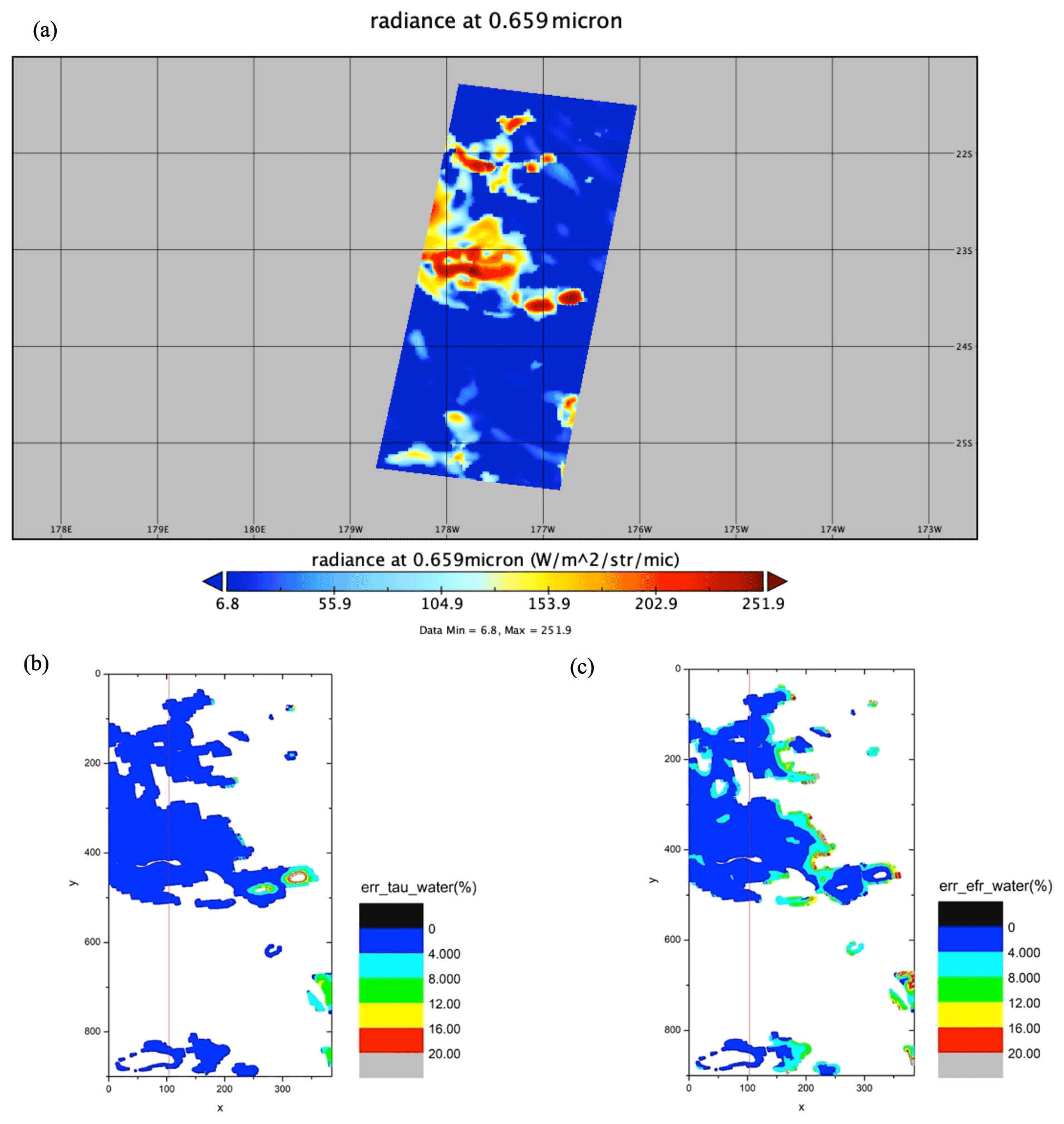
Figure 15NICAM/Joint-Simulator data for shallow warm clouds. (a) Radiance at 0.659 µm (band 1 of MSI), (b) error distribution of COT, and (c) error distribution of CDR. x and y in (b) and (c) show the pixel number in the swath or track direction. The red line in (b) and (c) stands for the location of the nadir.
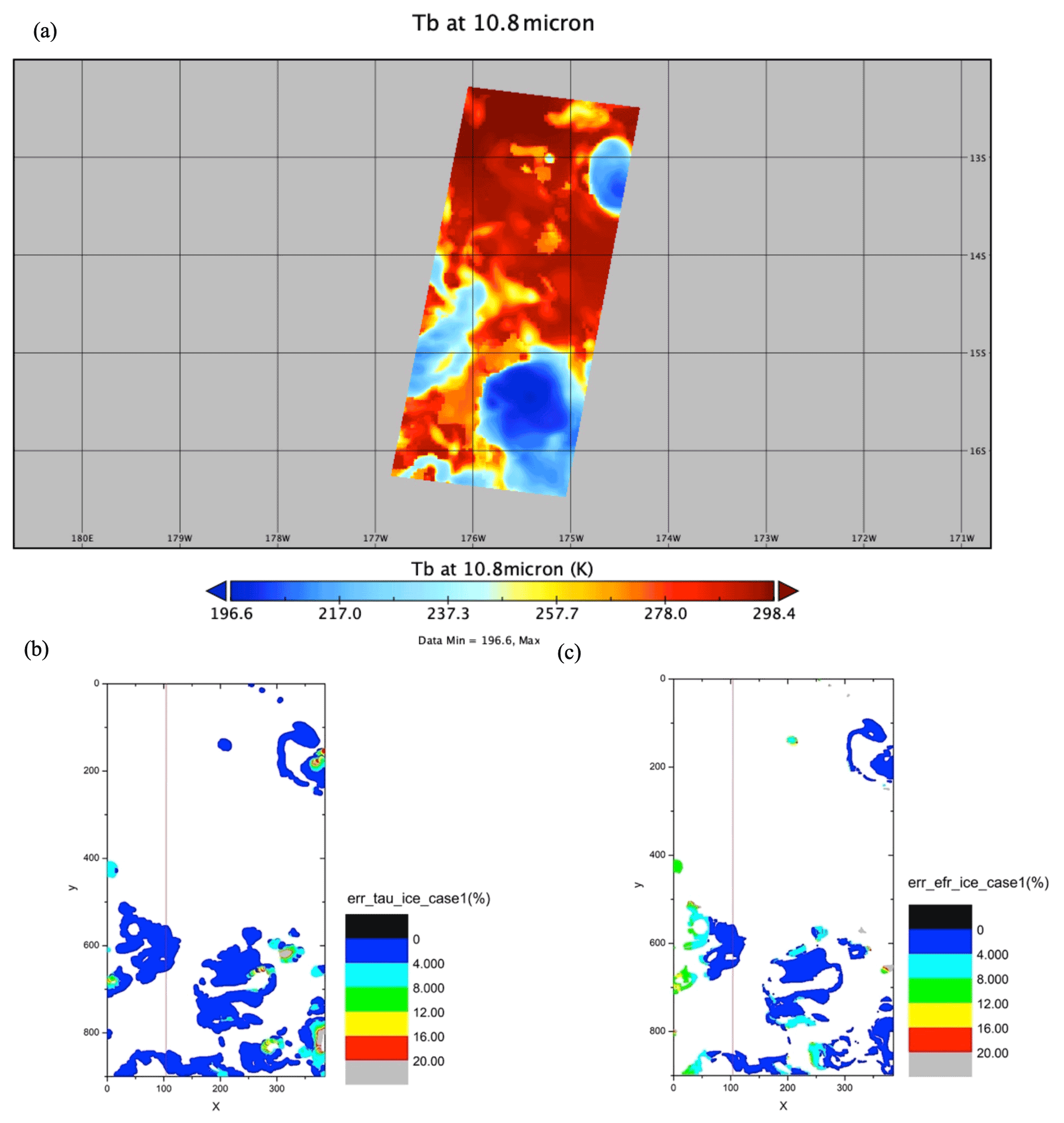
Figure 16NICAM/Joint-Simulator data for deep convective clouds. (a) Brightness temperature at 10.8 µm (band 6 of MSI), (b) error distribution of COT, and (c) error distribution of CDR. x and y in (b) and (c) show the pixel number in the swath or track direction. The red line in (b) and (c) stands for the location of the nadir.
For shallow warm clouds, 71 870 of the 344 064 pixels were defined as water clouds by the MSI cloud profiling algorithm. The average error of COT was 0.89 % and the standard deviation was 1.62 %, whereas the average error of CDR was 3.13 % and the standard deviation was 3.16 %.
For deep convective clouds, 29 501 of the 344 064 pixels were defined as ice cloud by the MSI cloud profiling algorithm. The average error of COT was 1.38 % and the standard deviation was 2.10 %, whereas the average error of CDR was 3.60 % and the standard deviation was 4.17 %.
The spatial distributions of Δτ and Δre are shown by Fig. 15b and c (shallow warm clouds) and Fig. 16b and c (deep convective clouds). x and y in Figs. 15b, c and 16b, c indicate the pixel number in the direction of the swath or track. The region around x = 20–100 and y = 850–900 in Fig. 15 is not defined as shallow warm clouds, whereas the error is off the scale in the region around x = 350 and y = 450. Comparing panel (a) with panels (b) and (c) in Figs. 15 and 16 showed that the MSI cloud profiling algorithm accurately identified the target clouds for both shallow warm clouds and deep convective clouds, and the shapes of the error distribution areas in panels (b) and (c) and the target cloud area in panel (a) matched well. The value of the response function at the nadir (the 102nd pixel) was the same, regardless of SMILE (Fig. 1). Therefore, our results also showed that Δτ and Δre were 0 at the 102nd pixel, and that the error tended to increase gradually from the nadir toward both sides, which was especially significant for deep convective cloud. Similar to the averaged error, Δre was larger than Δτ in the spatial distribution, but in most cases, both Δτ and Δre were less than 10 % (blue or light blue areas in Figs. 15 and 16). Although some pixels in Fig. 16c had Δre larger than 10 %, most of these pixels were the first and last 24 dummy pixels of the swath, meaning that the data from these pixels were unusable for the observations according to the specification of EarthCARE MSI.
Our results from the Nakajima–King diagram shown in Figs. 3 to 6 and Tables 3 to 4 also matched well with the results from NICAM/Joint-simulator data. The maximum value of Δτ was generally seen on pix_BND1_min for both shallow water cloud and deep convective cloud, and the maximum value of Δre was generally seen on pix_BND3_max for shallow water cloud but on pix_BND3_min for deep convective cloud. According to Tables 3 and 4, we found that for both types of cloud, Δτ on pix_BND1_min was generally larger than on pix_BND3_min, and Δre on pix_BND3_min was generally larger than on pix_BND1_min. This is basically because band 1 is more sensitive to COT and band 3 is more sensitive to CDR, suggesting that these extreme values of Δτ (2 %–4 %) and Δre (5 %–7 %) might be able to be referenced during actual observations. Our results from synthetic MSI data simulation proved this suggestion well.
Generally, the results of the NICAM/Joint-Simulator data matched those of the CAPCOM radiation transfer simulation well, suggesting that the error in COT and CDR caused by SMILE might be small, and could be regarded as negligible in most cases.
During the pre-launch phase of EarthCARE, numerous studies have been performed to characterize errors and ensure the accuracy of each observation instrument, in various aspects. As one of them, our work is based on both theoretical calculations and numerical simulations, providing scientific references for evaluating the influence of SMILE property as reasonably as possible. Furthermore, because SMILE could also be seen in other future optical instruments, our work also provided some typical examples of how the SMILE property affects the retrieval of cloud physical quantities. This provides a useful reference for the development of future cloud observation instruments.
According to our results for the CAPCOM radiation transfer simulation and observation scene simulation using NICAM/Joint-Simulator data, the Nakajima–King diagrams clearly showed the SMILE property on four chosen pixels of band 1 and band 3, as extreme values. Specifically, for typical shallow warm clouds (τ = 8, re = 8 µm), SMILE on the cloud retrieval was not significant in most cases (up to 6 % error), and for typical deep convective clouds (τ = 8, re = 40 µm), SMILE on the cloud retrieval was even less significant in most cases (up to 4 % error). Based on the sensitivity of each band to the retrieval of the physical quantity of each cloud, extreme error of COT (3.5 %) and CDR (6.3 %) were generally seen in band 1 and band 3 respectively. Furthermore, the synthetic MSI data provide not only the spatial distribution of COT/CDR error caused by SMILE property, but also a significant proof of our results from CAPCOM simulations. As the result did not exceed our evaluation criteria of 10 %, in most cases, we suggest that SMILE does not lead to appreciable errors in cloud retrieval data from EarthCARE MSI. This study suggests that an onboard correction of SMILE properties to the cloud profile algorithm is not necessary for MSI.
In CAPCOM, cloud top height (CTH) is determined by comparing cloud top temperature (CTT) with vertical temperature profile T(z), which is from global objective analysis data (e.g., ECMWF-AUX). Therefore, the error of CTH is ascribed to the error of CTT, directly. As this paper focuses on discussing SMILE on COT and CDR, we did not talk much about CTH or CTT. We believe that the error in CTH (and CTT) is expected to be small, at least to have little effect on the shortwave radiation budget. This is because CTT is related to the emissivity determined by the cloud characteristics, and the emissivity does not fluctuate so much, so we believe that SMILE does not affect the CTT very much.
However, our simulations in this study are based on observations over oceanic areas, which is much less strongly influenced by surface albedo than land areas. The surface albedo values used in the NICAM/Joint-Simulator data were 0.04–0.05, which did not change substantially throughout the scene. The surface reflectance could be much more complicated in observations over land areas. If the surface reflectance remained constant, it would be sufficient to correct for the albedo radiation. However, because surface reflectance is a function of the observation wavelength, the surface reflectance will affect the cloud retrieval. For the VIS channel (band 1 of MSI), which is close to the red edge of green vegetation, small shifts in the central wavelength can lead to uncertainties due to the rapid change in surface reflectance. Therefore, it requires more work to evaluate the effect of SMILE during cloud retrievals over land areas, and to determine whether SMILE is negligible everywhere.
Meanwhile, MSI is also used in the works of aerosol retrieval, which can also be affected by SMILE. As SMILE property on aerosol retrieval is beyond the scope of this study, future works on this evaluation are necessary too.
Finally, although the spatial resolution of NICAM (3.5 km) is lower than MSI, NICAM has its own advantage of simulating global areas. After focusing on two oceanic scenes in this study, our next task shall be to evaluate the whole orbit, showing the usefulness and potential of the NICAM data for future works.
Owing to the nature of this research, participants of this study did not agree for their data to be shared publicly; thus, supporting data are not available.
TYN and MS designed the basic framework of the simulations, and MW carried them out. TYN developed and provided the base model of CAPCOM, which was arranged for this study by MW. WR provided the synthetic MSI L1 data using NICAM/Joint-Simulator. KS provided the theoretical ground of the analytical estimation of shortwave radiation (Sect. 2.3). MY provided the wavelength distribution of relative response function on MSI bands 1 to 4 (Fig. 2). Gracious advices and helps from TK during the overall study. MW prepared the manuscript with contributions from all co-authors.
The contact author has declared that none of the authors has any competing interests.
Publisher's note: Copernicus Publications remains neutral with regard to jurisdictional claims in published maps and institutional affiliations.
This article is part of the special issue “EarthCARE Level 2 algorithms and data products”. It is not associated with a conference.
Special thanks to Tsuneaki Suzuki (now independent), who did the early part of this study as the predecessor of the corresponding author. Special thanks to ESA for providing the measured value of response functions of EarthCARE MSI.
This research has been supported by the Japanese Aerospace Exploration Agency (grant no. 22RT000087).
This paper was edited by Jian Xu and reviewed by two anonymous referees.
Albiñana, A. P., Gelsthorpe, R., Lefebvre, A., Sauer, M., Weih, E., Kruse, K., Münzenmayer, R., Baister, G., and Chang, M.: The multi-spectral imager on board the EarthCARE spacecraft, Infrared Remote Sensing and Instrumentation XVIII, edited by: Strojnik, M. and Paez, G., International Society for Optical Engineering, SPIE Proceedings, 7808, 780–815, https://doi.org/10.1117/12.858864, 2010.
Brenguier, J.-L., Burnet, F., and Geoffroy, O.: Cloud optical thickness and liquid water path – does the k coefficient vary with droplet concentration?, Atmos. Chem. Phys., 11, 9771–9786, https://doi.org/10.5194/acp-11-9771-2011, 2011.
Dadon, A., Ben-Dor, E., and Karnieli, A.: Use of derivative calculations and minimum noise fraction transform for detecting and correcting the spectral curvature effect (smile) in Hyperion Images, IEEE T. Geosci. Remote, 48, 2603–2612, https://doi.org/10.1109/TGRS.2010.2040391, 2010.
ESA: Technical note – MERIS smile effect characterization and correction, https://earth.esa.int/eogateway/documents/20142/37627/MERIS-Smile-Effect-Characterisation-and-correction.pdf (last access: 14 July 2021), 2008.
Fisher, J., Baumback, M., Bowles, J., Grosman, J., and Antoniades, J.: Comparison of low-cost hyperspectral sensors, Proc. SPIE, 3438, 23–30, 1998.
Green, R. O., Pavri, B. E., and Chrien, T. G.: On-orbit radiometric and spectral calibration characteristics of EO-1 Hyperion derived with an underflight of AVIRIS and in situ measurements at Salar de Arizaro, Argentina, IEEE T. Geosci. Remote, 41, 1194–1203, https://doi.org/10.1109/TGRS.2003.813204, 2003.
Hagihara, Y., Ohno, Y., Horie, H., Roh, W., Satoh, M., Kubota, T., and Oki, R.: Assessments of Doppler Velocity Errors of EarthCARE Cloud Profiling Radar Using Global Cloud System Resolving Simulations: Effects of Doppler Broadening and Folding, IEEE T. Geosci. Remote, 60, 1–9, https://doi.org/10.1109/TGRS.2021.3060828, 2021.
Hashino, T., Satoh, M., Hagihara, Y., Kubota, T., Matsui, T., Nasuno, T., and Okamoto, H.: Evaluating cloud microphysics from NICAM against CloudSat and CALIPSO, J. Geophys. Res.-Atmos., 118, 7273–7292, https://doi.org/10.1002/jgrd.50564, 2013.
Hashino, T., Satoh, M., Hagihara, Y., Kato, S., Kubota, T., Matsui, T., Nasuno, T., Okamoto, H., and Sekiguchi, M.: Evaluating Cloud Radiative Effects in Arctic simulated by NICAM with A-train, J. Geophys. Res.-Atmos., 121, 7041–7063, https://doi.org/10.1002/2016JD024775, 2016.
Illingworth, A., Barker, H., Beljaars, A., Ceccaldi, M., Chepfer, H., Delanoe, J., Domenech, C., Donovan, D., Fukuda, S., Hirakata, M., Hogan, R., Huenerbein, A., Kollias, P., Kubota, T., Nakajima, T., Nakajima, T., Nishizawa, T., Ohno, Y., and Okamoto, H.: The EARTHCARE satellite: The next step forward in global measurements of clouds, aerosols, precipitation and radiation, B. Am. Meteorol. Soc., 96, 1311–1332, https://doi.org/10.1175/BAMS-D-12-00227.1, 2015.
Ishida, H. and Nakajima, T. Y.: Development of an unbiased cloud detection algorithm for a spaceborne multispectral imager, J. Geophys. Res., 114, D07206, https://doi.org/10.1029/2008JD010710, 2009.
Japan Space Systems: Research and development of next-generation earth observation satellite utilization basic technology, https://warp.da.ndl.go.jp/info:ndljp/pid/11126101/www.meti.go.jp/meti_lib/report/2012fy/E002130.pdf (last access: 19 June 2021), 2012 (in Japanese).
JAXA: EarthCARE 1st Research Announcement (Validation), http://www.eorc.jaxa.jp/EARTHCARE/document/RA/1stRA_Val/EarthCARE_1stRA_Validation_english.pdf (last access: 6 September 2021), 2012.
JAXA: EarthCARE Level 2 Algorithm Theoretical Basis Document (L2 ATBD), http://www.eorc.jaxa.jp/EARTHCARE/document/reference/dev/EarthCARE_L2_ATBD.pdf, last access: 18 November 2021.
Kawamoto, K., Nakajima, T., and Nakajima, T. Y.: A global determination of cloud microphysics with AVHRR remote sensing, J. Climate, 14, 2054–2068, https://doi.org/10.1175/1520-0442(2001)014<2054:AGDOCM>2.0.CO;2, 2001.
Kikuchi, M., Oki, R., Kubota, T., Yoshida, M., Hagihara, Y., Takahashi, C., Ohno, Y., Nishizawa, T., Nakajima, T. Y., Suzuki, K., Satoh, M., Okamoto, H., and Tomita, E.: Overview of Earth, Clouds, Aerosols and Radiation Explorer (EarthCARE) – Integrative Observation of Cloud and Aerosol and Their Radiative Effects on the Climate System, J. Remote Sens. Soc. Japan, 39, 181–196, https://doi.org/10.11440/rssj.39.181, 2019 (in Japanese).
Koopman, R. (Ed.): EarthCARE instruments description, European Space Research and Technology Centre, https://earth.esa.int/eogateway/documents/20142/37627/EarthCARE-instrument-descriptions.pdf (last access: 14 November 2021), 2017.
Kubota, T., Seto, S., Satoh, M., Nasuno, T., Iguchi, T., Masaki, T., Kwiatkowski, J. M., and Oki, R.: Cloud assumption of Precipitation Retrieval Algorithms for the Dual-frequency Precipitation Radar, J. Atmos. Ocean. Technol., 37, 2015–2031, https://doi.org/10.1175/JTECH-D-20-0041.1, 2020.
Letu, H., Ishimoto, H., Riedi, J., Nakajima, T. Y., C.-Labonnote, L., Baran, A. J., Nagao, T. M., and Sekiguchi, M.: Investigation of ice particle habits to be used for ice cloud remote sensing for the GCOM-C satellite mission, Atmos. Chem. Phys., 16, 12287–12303, https://doi.org/10.5194/acp-16-12287-2016, 2016.
Letu, H., Nagao, T. M., Nakajima, T. Y., Ishimoto, H., Riedi, J., Baran, A., Shang, H., Sekiguchi, M., and Kikuchi, M.: Ice cloud properties From Himawari-8/AHI next-generation geostationary satellite: capability of the AHI to monitor the DC cloud generation process, IEEE T. Geosci. Remote, 57, 3229–3239, https://doi.org/10.1109/TGRS.2018.2882803, 2019.
Masunaga, H., Matsui, T., Tao, W.-K., Hou, A. Y., Kummerow, C. D., Nakajima, T., Bauer, P., Olson, W. S., Sekiguchi, M., and Nakajima, T. Y.: Satellite Data Simulator Unit: A multisensor, multispectral satellite simulator package, B. Am. Meteorol. Soc., 91, 1625–1632, https://doi.org/10.1175/2010BAMS2809.1, 2010.
Matsui, T., Zeng, X., Tao, W.-K., Masunaga, H., Olson, W., and Lang, S.: Evaluation of long-term cloud-resolving model simulations using satellite radiance observations and multifrequency satellite simulators, J. Atmos. Ocean. Technol., 26, 1261–1274, https://doi.org/10.1175/2008JTECHA1168.1, 2009.
Matsui, T., Iguchi, T., Li, X., Han, M., Tao, W., Petersen, W., L'Ecuyer, T., Meneghini, R., Olson, W., Kummerow, C. D., Hou, A. Y., Schwaller, M. R., Stocker, E. F., and Kwiatkowski, J.: GPM satellite simulator over ground validation sites, B. Am. Meteorol. Soc., 94, 1653–1660, https://doi.org/10.1175/BAMS-D-12-00160.1, 2013.
Matsui, T., Tao, W.-K., Chern, J., Lang, S., Satoh, M., Hashino, T., and Kubota, T.:On the Land-Ocean Contrast of Tropical Convection and Microphysics Statistics Derived from TRMM Satellite Signals and Global Storm-Resolving Models, J. Hydrometeorol., 17, 1425–1445, https://doi.org/10.1175/JHM-D-15-0111.1, 2016.
Mouroulis, P., Green, R., and Chrien, T.: Design of pushbroom imaging spectrometers for optimum recovery of spectroscopic and spatial information, Appl. Optics, 39, 2210–2220, 2000.
Nakajima, T. and King, M. D.: Determination of the optical thickness and effective particle radius of clouds from reflected solar radiation measurements. Part I: Theory, J. Atmos. Sci., 47, 1878–1893, https://doi.org/10.1175/1520-0469(1990)047<1878:DOTOTA>2.0.CO;2, 1990.
Nakajima, T. and Tanaka, M.: Matrix formulations for the transfer of solar radiation in a plane-parallel scattering atmosphere, J. Quant. Spectrosc. Ra., 35, 13–21, https://doi.org/10.1016/0022-4073(86)90088-9, 1986.
Nakajima, T. and Tanaka, M.: Algorithms for radiative intensity calculations in moderately thick atmospheres using a truncation approximation, J. Quant. Spectrosc. Ra., 40, 51–69, https://doi.org/10.1016/0022-4073(88)90031-3, 1988.
Nakajima, T., King, M. D., Spinhirne, J. D., and Radke, L. F.: Determination of the optical thickness and effective particle radius of clouds from reflected solar radiation measurements. Part II: Marine stratocumulus observations, J. Atmos. Sci., 48, 728–750, https://doi.org/10.1175/1520-0469(1991)048<0728:DOTOTA>2.0.CO;2, 1991.
Nakajima, T. Y. and Nakajima, T.: Wide-area determination of cloud microphysical properties from NOAA AVHRR measurements for FIRE and ASTEX regions, J. Atmos. Sci., 52, 4043–4059, https://doi.org/10.1175/1520-0469(1995)052<4043:WADOCM>2.0.CO;2, 1995.
Nakajima, T. Y., Nakajima, T., Nakajima, M., Fukushima, H., Kuji, M., Uchiyama, A., and Kishino, M.: Optimization of the Advanced Earth Observing Satellite II Global Imager channels by use of radiative transfer calculations, Appl. Optics, 37, 3149–3163, https://doi.org/10.1364/AO.37.003149, 1998.
Nakajima, T. Y., Murakami, H., Hori, M., Nakajima, T., Aoki, T., Oishi, T., and Tanaka, A.: Efficient use of an improved radiative transfer code to simulate near-global distributions of satellite-measured radiances, Appl. Optics, 42, 3460–3471, https://doi.org/10.1364/AO.42.003460, 2003.
Nasuno, T., Yamada, H., Nakano, M., Kubota, H., Sawada, M., and Yoshida, R.: Global cloud-permitting simulations of Typhoon Fengshen (2008), Geosci. Lett., 3, 1–13, https://doi.org/10.1186/s40562-016-0064-1, 2016.
Roh, W. and Satoh, M.: Evaluation of precipitating hydrometeor parameterizations in a single-moment bulk microphysics scheme for deep convective systems over the tropical central Pacific, J. Atmos. Sci., 71, 2654–2673, https://doi.org/10.1175/JAS-D-13-0252.1, 2014.
Roh, W. and Satoh, M.: Extension of a multisensor satellite radiance-based evaluation for cloud system resolving models, J. Meteorol. Soc. Jpn. Ser. II, 96, 55–63, https://doi.org/10.2151/jmsj.2018-002, 2018.
Roh, W., Satoh, M., and Nasuno, T.: Improvement of a cloud microphysics scheme for a global nonhydrostatic model using TRMM and a satellite simulator, J. Atmos. Sci., 74, 167–184, https://doi.org/10.1175/JAS-D-16-0027.1, 2017.
Roh, W., Satoh, M., Hashino, T., Okamoto, H., and Seiki, T.: Evaluations of the thermodynamic phases of clouds in a cloud-system-resolving model using CALIPSO and a satellite simulator over the Southern Ocean, J. Atmos. Sci., 77, 3781–3801, https://doi.org/10.1175/JAS-D-19-0273.1, 2020.
Satoh, M., Matsuno, T., Tomita, H., Miura, H., Nasuno, T., and Iga, S.: Nonhydrostatic ICosahedral Atmospheric Model (NICAM) for global cloud resolving simulations, J. Comput. Phys., 227, 3486–3514, https://doi.org/10.1016/j.jcp.2007.02.006, 2008.
Satoh, M., Inoue, T., and Miura, H.: Evaluations of cloud properties of global and local cloud system resolving models using CALIPSO and CloudSat simulators, J. Geophys. Res.-Atmos., 115, D00H14, https://doi.org/10.1029/2009JD012247, 2010.
Satoh, M., Tomita, H., Yashiro, H., Miura, H., Kodama, C., Seiki, T., Noda, A. T., Yamada, Y., Goto, D., Sawada, M., Miyoshi, T., Niwa, Y., Hara, M., Ohno, T., Iga, S., Arakawa, T., Inoue, T., and Kubokawa, H.: The Non-hydrostatic Icosahedral Atmospheric Model: description and development, Prog. Earth Planet. Sci., 1, 1–32, https://doi.org/10.1186/s40645-014-0018-1, 2014.
Satoh, M., Roh, W., and Hashino, T.: Evaluations of clouds and precipitations in NICAM using the Joint Simulator for Satellite Sensors, CGER's Supercomputer Monograph Report, 22, 110, ISSN 1341-4356, CGER-I127-2016, 2016.
Solomon, S., Qin, D.,, Manning, M., Chen, Z., Marquis, M., Averyt, K. B., Tignor, M., and Miller, H. L. (Eds.): Climate Change 2007: The Physical Science Basis. Contribution of Working Group I to the Fourth Assessment Report of the Intergovernmental Panel on Climate Change, Cambridge University Press, Cambridge, United Kingdom and New York, USA, https://www.ipcc.ch/site/assets/uploads/2018/02/ar4-wg1-spm-1.pdf (last access: 13 November 2021), 2007.
Stamnes, K., Tsay, S.-C., Wiscombe, W., and Jayaweera, K.: Numerically stable algorithm for discrete-ordinate-method radiative transfer in multiple scattering and emitting layered media, Appl. Optics, 27, 2502–2509, https://doi.org/10.1364/AO.27.002502, 1988.
Tomita, H.: New microphysical schemes with five and six categories by diagnostic generation of cloud ice, J. Meteorol. Soc. Jpn., 86A, 121–142, https://doi.org/10.2151/jmsj.86A.121, 2008.
Tomita, H. and Satoh, M.: A new dynamical framework of nonhydrostatic global model using the icosahedral grid, Fluid Dyn. Res., 34, 357–400, https://doi.org/10.1016/j.fluiddyn.2004.03.003, 2004.
Yamada, H., Nasuno, T., Yanase, W., and Satoh, M.: Role of the vertical structure of a simulated tropical cyclone in its motion: a case study of Typhoon Fengshen (2008), Sci. Online Lett. Atmos., 12, 203–208, https://doi.org/10.2151/sola.2016-041, 2016.
Yokota, N., Miyamura, N., and Iwasaki, A.: Preprocessing of hyperspectral imagery with consideration of smile and keystone properties, Proc. SPIE, 7857, 78570B, https://doi.org/10.1117/12.870437, 2010.