the Creative Commons Attribution 4.0 License.
the Creative Commons Attribution 4.0 License.
 | 22 Dec 2023
Multi-star calibration in starphotometry
Liviu Ivănescu
Norman T. O'Neill
We explored the improvement in starphotometry accuracy using a multi-star Langley calibration in lieu of the more traditional one-star Langley approach. Our goal was a 0.01 calibration-constant repeatability accuracy, at an operational sea-level facility such as our Arctic site at Eureka. Multi-star calibration errors were systematically smaller than single-star errors and, in the mid-spectrum, approached the 0.01 target for an observing period of 2.5 h. Filtering out coarse-mode (supermicrometre) contributions appears mandatory for improvements. Spectral vignetting, likely linked to significant UV/blue spectrum errors at large air mass, may be due to a limiting field of view and/or sub-optimal telescope collimation. Starphotometer measurements acquired by instruments that have been designed to overcome such effects may improve future star magnitude catalogues and consequently starphotometry accuracy.
- Article
(5873 KB) - Full-text XML
- BibTeX
- EndNote


Starphotometry involves the measurement of attenuated starlight in semi-transparent atmospheres as a means of extracting the spectral optical depth and thereby estimating columnar properties of absorbing and scattering constituents such as aerosols, trace gases and optically thin clouds. Dedicated instrument development already began in the late 1950s (Dachs, 1960, 1966; Dachs et al., 1966), with increased activity after 2000 (Théorêt, 2003; Gröschke et al., 2009; Pérez Ramírez, 2010; Oh, 2015). One of the earliest comprehensive investigations of starphotometry errors and their influence on calibration was reported in the astronomical literature by Young (1974). Calibration strategies for retrieving accurate photometric observations in variable optical depth conditions were proposed by Rufener (1964, 1986). Those studies were recently updated and complemented using measurements from our High Arctic, sea-level observatory at Eureka, NU, Canada (Ivănescu, 2015; Baibakov et al., 2015; Ivănescu et al., 2021), using a commercial-spectrometer-based starphotometer1, attached to a Celestron C11 telescope. This, more recent, work underscored certain challenges in performing calibration at such a high-latitude/low-altitude site. The remoteness of the Eureka site and the significant infrastructure requirements of the starphotometer render calibration campaigns at a dedicated mountain site, onerous. The alternative to a calibration campaign (particularly at an Arctic site like Eureka) is to improve on-site calibration methods by overcoming the relatively large optical depth variability typical of operational sites. Much can be learned by exploring this option at an Arctic location like Eureka (see O'Neill et al., 2016, for a discussion of optical depth variability).
Star-dependent (one-star) Langley calibration that depends on large air mass variations is the current standard in starphotometry (see Pérez-Ramírez et al., 2008, 2011). This is mainly due to the limited accuracy of available extraterrestrial star magnitudes (Ivănescu et al., 2021). A good number of High Arctic stars cannot, however, be calibrated in such a way since they do not go through large elevation (i.e. air mass) changes (in the extreme case of a site at the pole, there are no elevation changes). Our goal is to demonstrate that a sub-0.01 optical depth error (partly linked to calibration errors) can be achieved by performing the type of instrument-dependent, star-independent calibration referred to in Ivănescu et al. (2021).
2.1 Langley calibration
The starphotometer retrieval algorithm is based on extraterrestrial and atmospherically attenuated magnitudes of non-variable bright stars, denoted by M0 (provided by the Pulkovo catalogue of Alekseeva et al., 1996) and M, respectively (see Ivănescu et al., 2021, for a more comprehensive elaboration of this section). Their corresponding instrument signals, expressed in terms of magnitude, are and , respectively, with F0 and F being the actual measurements in counts s−1. The star-independent conversion factor between the catalogue and instrument magnitudes is (Ivănescu et al., 2021)
The C factor accounts for the optical and electronic throughput of the starphotometer, as well as the photometric system transformation between the instrument signal magnitude and the extraterrestrial catalogue magnitude. In terms of magnitude, the Beer–Bouguer–Lambert atmospheric attenuation law is
where m is the observed air mass, and τ is the total optical depth. Inserting Eq. (1) yields
where . This expression can be used to retrieve C from a linear regression of M0−S versus x, if τ is assumed constant. Such a procedure is referred to as the Langley calibration technique or Langley plot. In the absence of an accurate M0 spectrum, Eq. (2) can be used to transform Eq. (4) into
for which a catalogue is no longer required. This linear regression enables the retrieval of S0 instead of C and thus represents a star-dependent calibration.
The right side of Eq. (4) notably indicates that M0−S is star independent: it thus represents a linear regression that any star can contribute to and, accordingly, a framework for multi-star Langley calibration.
3.1 Measurement accuracy
The differential of (rearranged) Eq. (4) yields the calibration accuracy error:
The (δxτ+xδτ) component underscores the rationale for performing calibrations at a high-altitude site (where τ, δτ and δxτ are typically smaller) and the advantage of maintaining small x in order to minimize the xδτ contribution to δC. The sky stability during the retrieval of C may be monitored by computing τ for each sample, with Eq. (4). The δS error component accounts for any systematic signal changes: optical transmission degradation, misalignment error and star spot vignetting, etc. The component accounts for any magnitude bias in the bright-star catalogue (i.e. the average of accuracy-error spectra for all catalogue stars: see Ivănescu et al., 2021, for a detailed discussion of error bias in the Pulkovo and other catalogues). Because it is a catalogue-specific constant, the optical depth retrieval accuracy will not be affected by its consistent use2.
3.2 Regression precision
A linear regression applied to a plot of versus x yields the slope () and intercept () of the Langley Eq. (4). The regression equation is then , and the linear-fit residuals are represented by . The standard error of the regression slope and intercept for a large number of measurements3 can be expressed as (see, for example, Montgomery and Runger, 2011)
It should be noted that (the mean of the residual) =0 is a corollary of the linear regression constraints.
The Langley calibration y axis embodies two independent sets of measurements: N “measurements” of M0 and n measurements of S. From a pure-noise standpoint, the residuals can be represented by an ensemble of individual measurements () where each parameter (except C) is subject to noisy variation. Excluding the typically negligible random errors in x yields4
where the standard error expression for a linear combination of random variables was employed (Barford, 1985). The subscript ϵ represents a single instance of a random (noise) measurement in S, τ or M0, and σϵ is its zero-mean standard deviation. was replaced by στ because no systematic variation was assumed in τ during the calibration period. represents the difference between an individual star's M0 accuracy errors and the averaged M0 catalogue bias. The term is specific for the use of multiple stars during the calibration.
The assumption of constant τ in time (t) and observational direction (expressed in terms of m) may be problematic over long observation periods and large air mass changes. It is a useful exercise to assess the average time period and air mass range over which a degree of τ constancy (sky stability) is maintained.
Variations of a sky instability parameter (σδτ) were analyzed using δτ differences for τ measurements acquired during the 2019–2020 season in Eureka. δτ values were placed into (a) fixed Δt bins to generate δτ histograms for high stars (where is computed from a later time (f) relative to an earlier time (i)) and (b) fixed Δm bins from high- to low-star m pairs. Since δ values of each bin generally come from distinct periods, τf and τi are expected to be uncorrelated: the τi versus τf correlation coefficient was determined to be <0.25 when τp<0.1, Δt<1 h and ∼0.1 otherwise (see the legend of Fig. 1 for the definition of τp). This is negligible for the purposes of our analysis, and, accordingly, they can be considered as independent variables. The approximation (Soch et al., 2021) can accordingly be employed for each Δm or Δt bin.
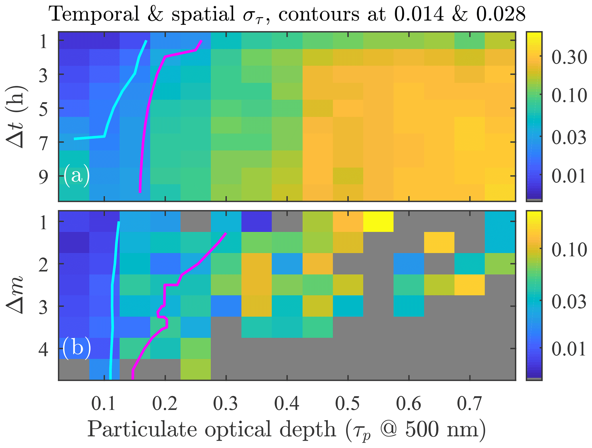
Figure 1Two-dimensional sky instability (στ) patterns for the 2019–2020 season at Eureka. The colour-coded στ values are computed relative to a reference τ value but plotted as a function of its associated particulate optical depth (, where τm is the molecular scattering optical depth) and (a) time difference (Δt) or (b) air mass difference (Δm). The magenta and purple curves represent the column-wise averaged στ=0.014 and 0.028 contour lines. There were many more data associated with Δt than with Δm bins (i.e. more robust bin statistics are expected in the former case). Note that Δm and Δt were chosen to be positive.
Those histograms often included anisotropic outliers typical of lognormal τ statistics (Sayer and Knobelspiesse, 2019). A median approach was chosen to render the statistics approximately independent of the outliers: the MAD (median absolute deviation) parameter was employed as a robust measure of histogram width (see Eq. 1.3 in Rousseeuw and Croux, 1993, for MAD details). In order to eventually convert the statistics to those of a normal distribution, an outlier cutoff of 4.5⋅MAD was defined5. This particular cutoff is equivalent to the classical normal distribution outlier cutoff of 3σ since .
Figure 1 shows στ (computed after the outlier cutoff and using the στ approximation given above) as a function of (a) Δt and (b) Δm. It can be shown6 that a calibration period of 2 h, for which n≃46 at the standard sampling rate of starphotometer, yields . This means that the calibration error () is limited to <0.01 only if στ<0.014. An 8 h observing period enables a more generous limit of στ<0.028 to achieve the same calibration precision. Contour curves of στ=0.014 and 0.028 are superimposed on Fig. 1.
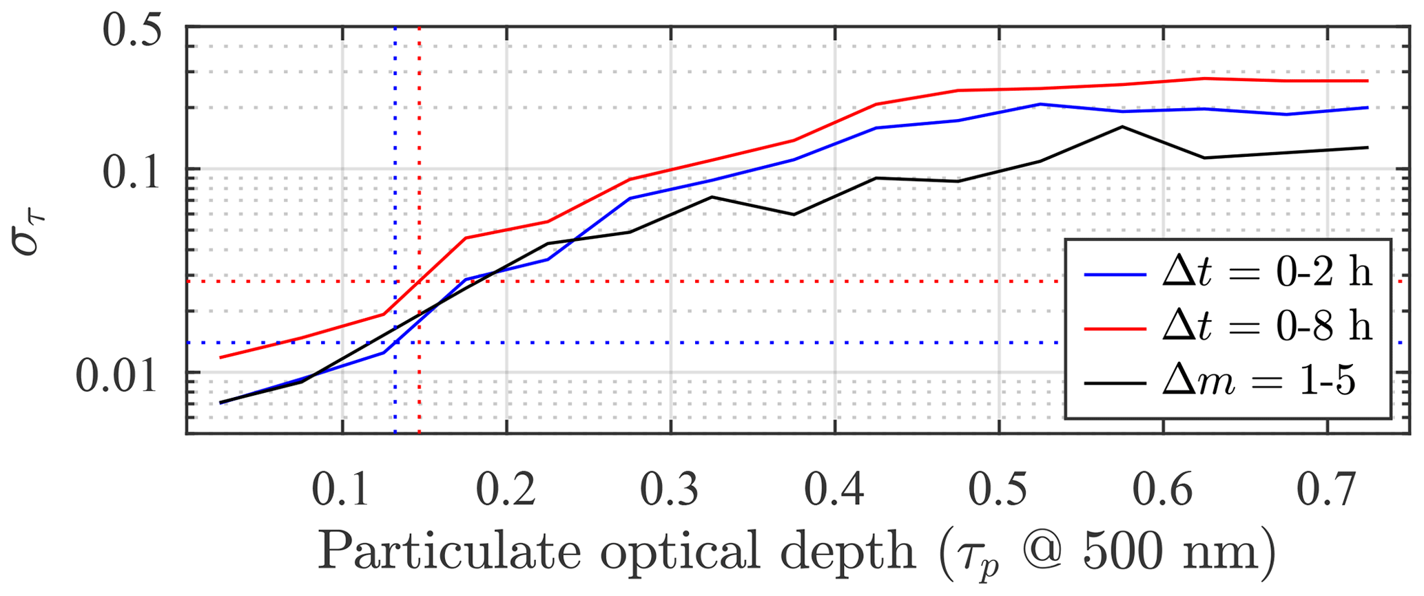
Figure 2 shows the στ variability estimation for the 2 h “fast” and the 8 h “long” calibration periods, as well as a third scenario with Δm=1 to 5. The three curves represent the standard deviation (after cutoff) of the corresponding range-aggregated data. They tend to converge with decreasing τp: the 2 h and 8 h στ values of 0.014 and 0.028 correspond to τp values of 0.13 and 0.15, respectively (vertical dashed blue and red lines defined by the intersection with the corresponding horizontal 0.014 and 0.028 lines). The cases τp≤0.13 and 0.15 were labelled as “clear-sky” conditions because of their tendency to promote calibration stability. Their corresponding clear-sky statistics are presented in Appendix A.
Many High Arctic stars are circumpolar (i.e. they never set), and thus their air mass range is limited. Figure 3 shows air mass variation as a function of time past the transit for our dataset of the 13 brightest (and stable) stars at Eureka.
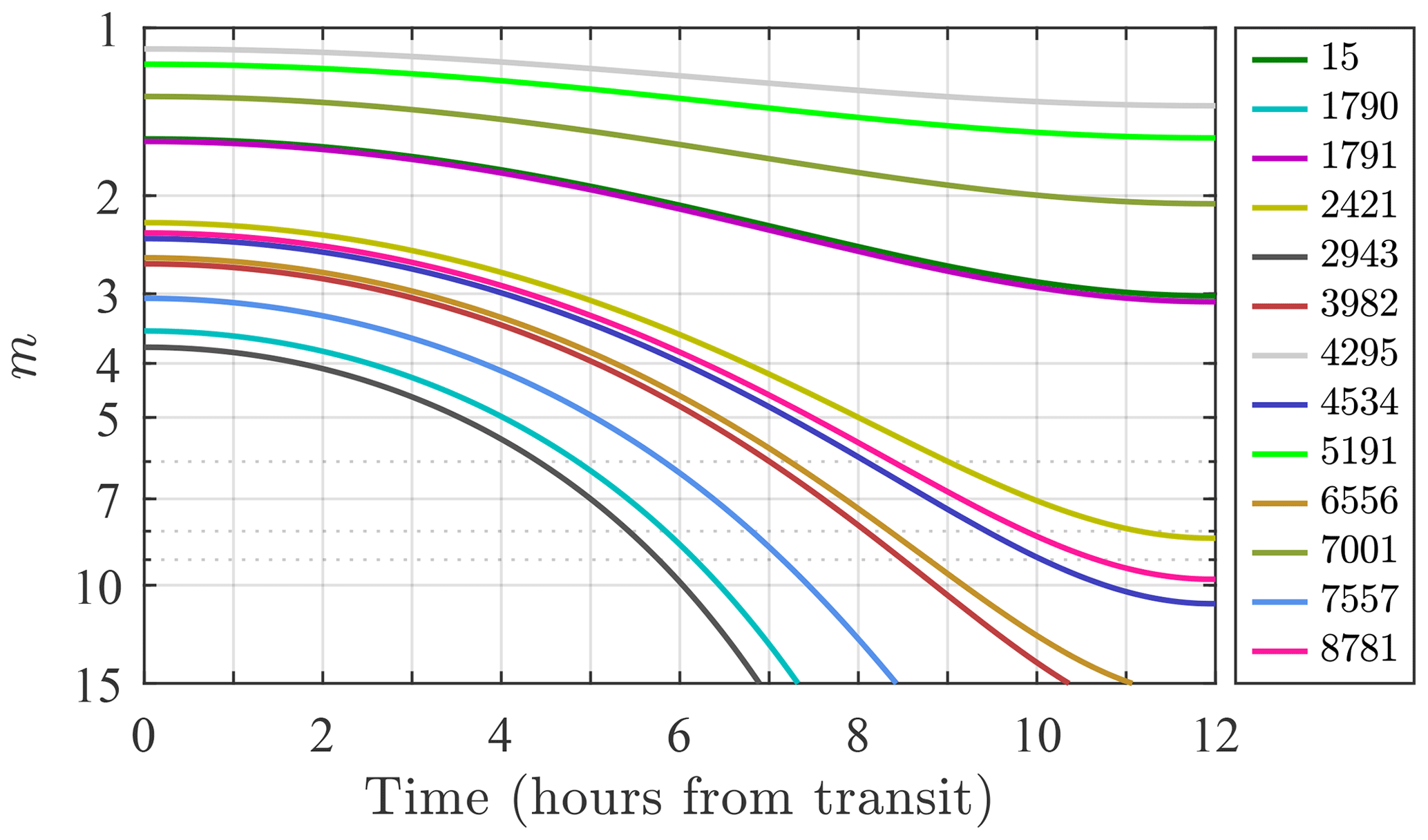
Figure 3Air mass versus time past the transit for the bright stars observable at Eureka (identified by their HR catalogue index). The transit of a given star occurs when it crosses the local meridian (minimum air mass).
A well-defined separation is notable between high stars (m(12 h)<3.1) and low stars (m(0 h)>2.2). A large air mass range is clearly only available for the low stars (i.e. about two-thirds of our Eureka bright-star dataset). However, star vignetting, due to turbulence-inducing star-spot expansion beyond the boundaries of the field of view (FOV), may affect the optical throughput of the Eureka system at m>5 (Ivănescu et al., 2021). This type of air mass constraint, combined with the low-star constraints of Fig. 3, results in only moderate Δm excursions (at the expense of substantial Δt) if only a single star is employed in a Langley-type calibration. A multi-star calibration can be exploited to mitigate such Δm and Δt limitations.
This type of calibration exploits a singular advantage of starphotometry over moonphotometry and sunphotometry: the capability of employing multiple extraterrestrial light sources in a relatively short period of time. In comparison with a C-determining Langley calibration using one star, the multi-star approach enables a synergistic Langley calibration that employs several stars exhibiting a wide range of air mass values over a significantly shorter period of time.
One- and multi-star Langley calibrations acquired with the Eureka starphotometer on 7 December 2019 and 10 January 2020, respectively, are shown in Fig. 4. The observations for x>5 were carried out to highlight any vignetting effect due to the aforementioned star-spot expansion. The one-star case (small black dots and their associated “1-lin” regression line) shows the results for the low Procyon star (HR 2943, spectral type F5V). Its colder temperature ensures a near-infrared (NIR) brightness that is larger than all the other bright stars of Fig. 37. That reason aside, it is also, arguably, the most optimal one-star Langley-regression choice since no other Fig. 3 bright star can duplicate its large and rapid air mass change (see the lowest black curve).
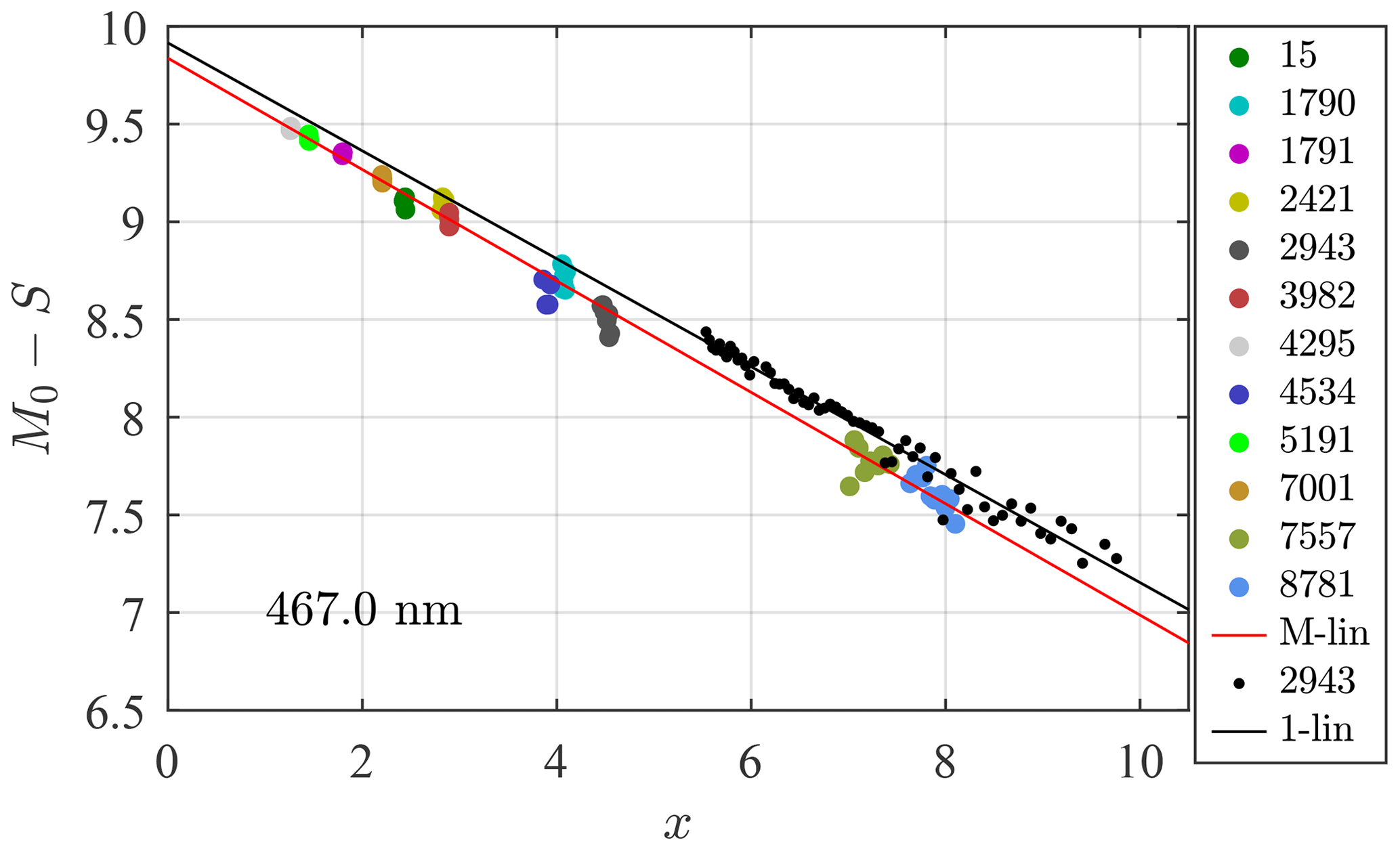
Figure 4One- and multi-star Langley calibrations (both lasting about 2.5 h; see Appendix A). The one-star and multi-star measurement points are represented, respectively, by small black dots and large solid-coloured circles, while their linear regression fits appear as solid lines (1-lin and M-lin, respectively). Each point represents an average of five 6 s exposures. Each star is identified by their HR IDs (see Table B1 in Ivănescu et al., 2021).
5.1 Calibration precision
The resulting one- and multi-star spectra (each spectral point representing a linear-regression Langley slope) are shown in Fig. 5a. Their associated precision errors () of Eq. (7) are shown in Fig. 5b. One should note that the estimated multi-star error is substantially and consistently smaller than that of the one-star calibration. The and spectra from the Langley regressions are shown in Fig. 6a and b, respectively. The values are, in the multi-star case, significantly smaller and closer to the 0.01 target.
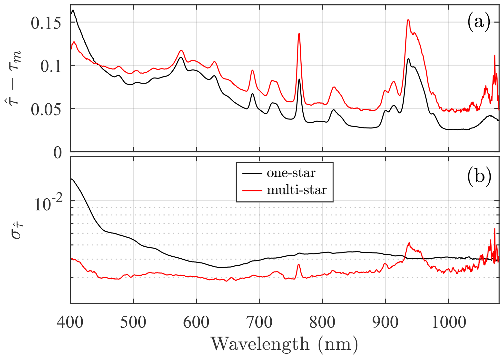
Figure 5(a) One- and multi-star Langley-regression slopes (expressed as ). (b) values derived from Eq. (7).
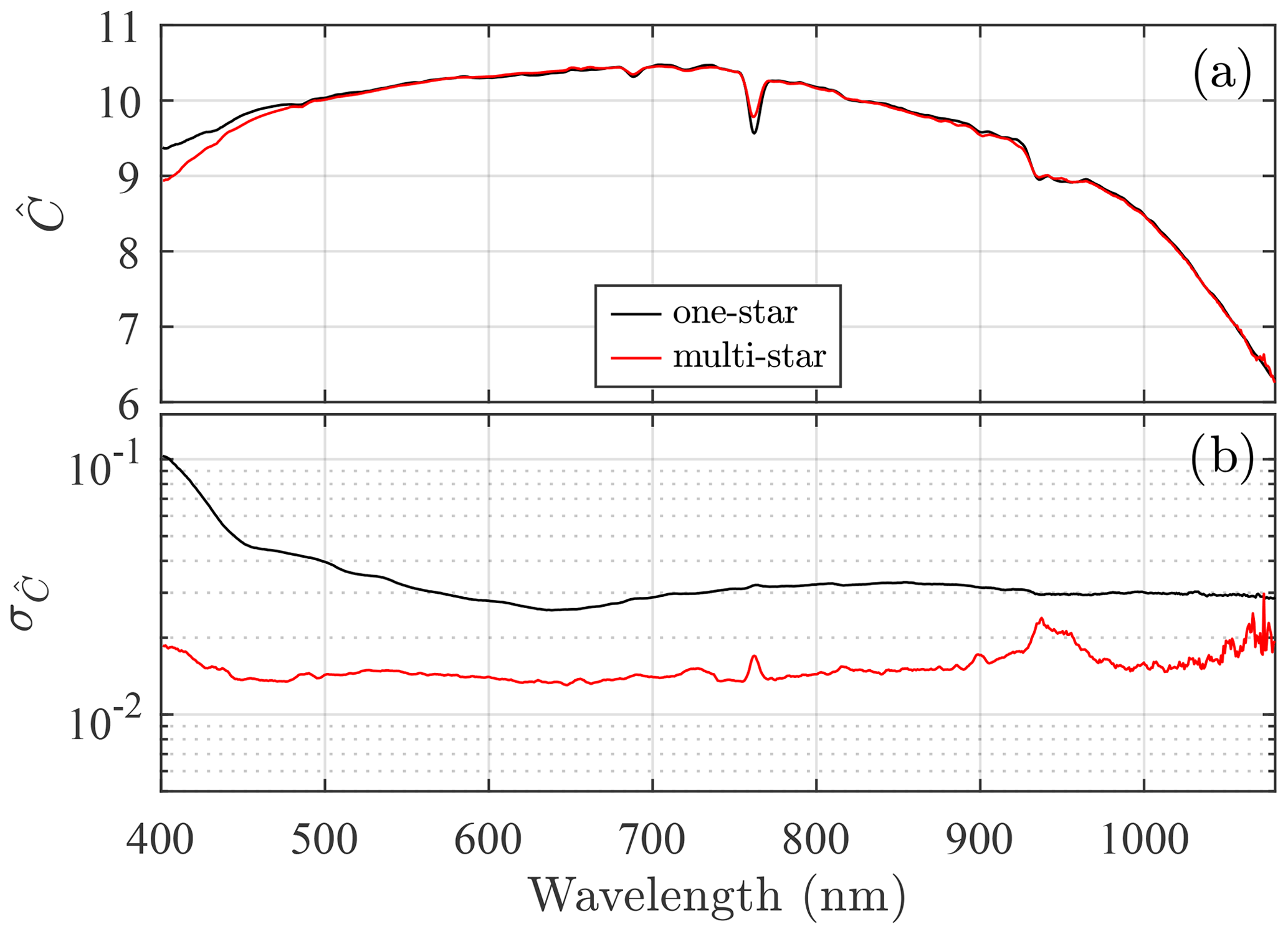
Figure 6(a) retrieved from the one- and multi-star Langley calibrations. (b) values computed using Eq. (7).
The generally smaller values of the multi-star case are partly attributable to the one-star case being limited to a relatively smaller x range (i.e. smaller σx in Eq. 7), while the smaller values are partly attributable to the smaller values and the lower values of (see Eq. 7). The increases in the ultraviolet (UV) and NIR are discussed in Sect. 6.2. The peak around 940 nm is likely associated with a faint and noisy star signal induced by strong attenuation in the water vapour absorption band, coupled with the non-linear nature of the optical depth in that spectral region (Pérez-Ramírez et al., 2012).
5.2 Repeatability
The robustness of the spectra of Fig. 6b and the impact of potential systematic errors can be investigated with repeatability experiments. The spectra employed to produce the standard deviations8 shown in Fig. 7 were derived from three one-star and three multi-star Langley calibrations that were well separated in time (i.e. they were optically independent in terms of any significant correlations between the τp variations of each period) and nearly satisfied the clear-sky calibration constraints of Sect. 4. The Fig. 7 error spectra are, with the exception of larger differences in certain spectral regions, roughly coherent with the Fig. 6b spectra (including the fact that the one-star errors are significantly larger than the multi-star errors).
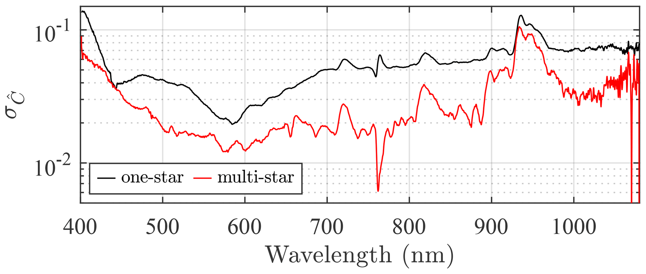
Figure 7 curves derived for three one-star Langley calibrations acquired using the Procyon (HR 2943) star on 7 December 2019, 5 January 2020 and 16 January 2020, as well as three multi-star calibrations acquired on 10 March 2018, 7 December 2019 and 10 January 2020. These spectra are generally similar to Fig. 6b results.
6.1 Data processing
Figure 8 shows dual-wavelength (400 and 1000 nm) regression tests for two of the three one-star calibrations of the previous section (two of the three dates given in the legend of Fig. 7 for the HR 2943 star) plus a third hotter star (HR 3982, spectral type B7) that was specifically chosen to better understand the influence of temperature-driven spectral differences in the target star. The smaller regression slope and point dispersion about the HR 3982 regression line, compared with the two HR 2943 cases, are noticeable at both wavelengths (notably at 1000 nm) and are an indicator of generally clearer sky conditions.
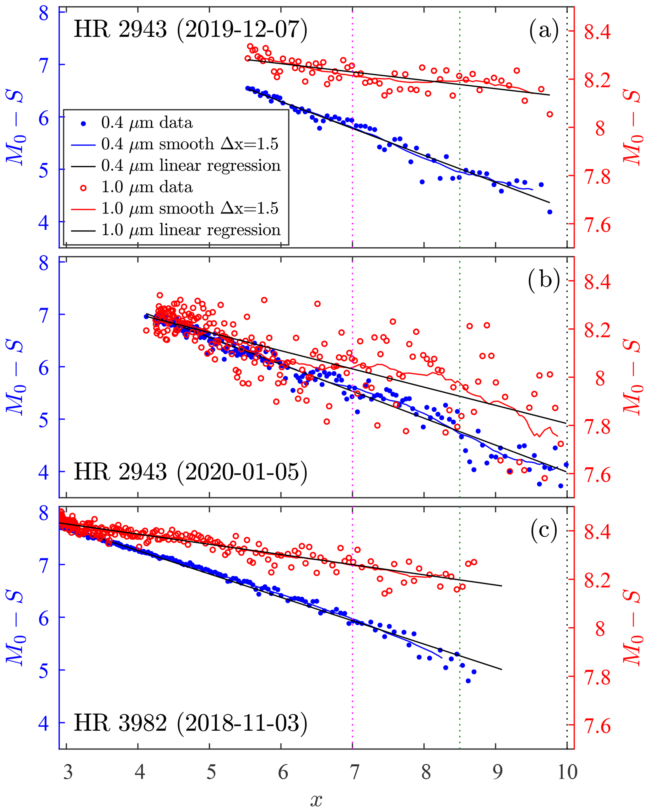
Figure 8One-star calibrations at two spectrally distinct channels (400 and 1000 nm) for different dates and stars. The black lines represent the full regression line for all data points over the entire x range. Star measurements for the (a) and (b) cases started at the smallest x values, while the (c) case measurements began at the largest x value. The solid (varying) curves were generated by averaging (M0−S) over Δx=1.5 sliding windows. The three coloured (dotted) vertical lines correspond to the colours of the three xmax cases of Fig. 10.
The C values retrieved from linear regressions over an increasing x range in Fig. 8 (from the smallest x value to an artificial maximum of xmax) are plotted in Fig. 9. The damping out of regression noise and the asymptotic approach to the horizontal pan-x regression value as xmax increases can be readily observed in all three plots.
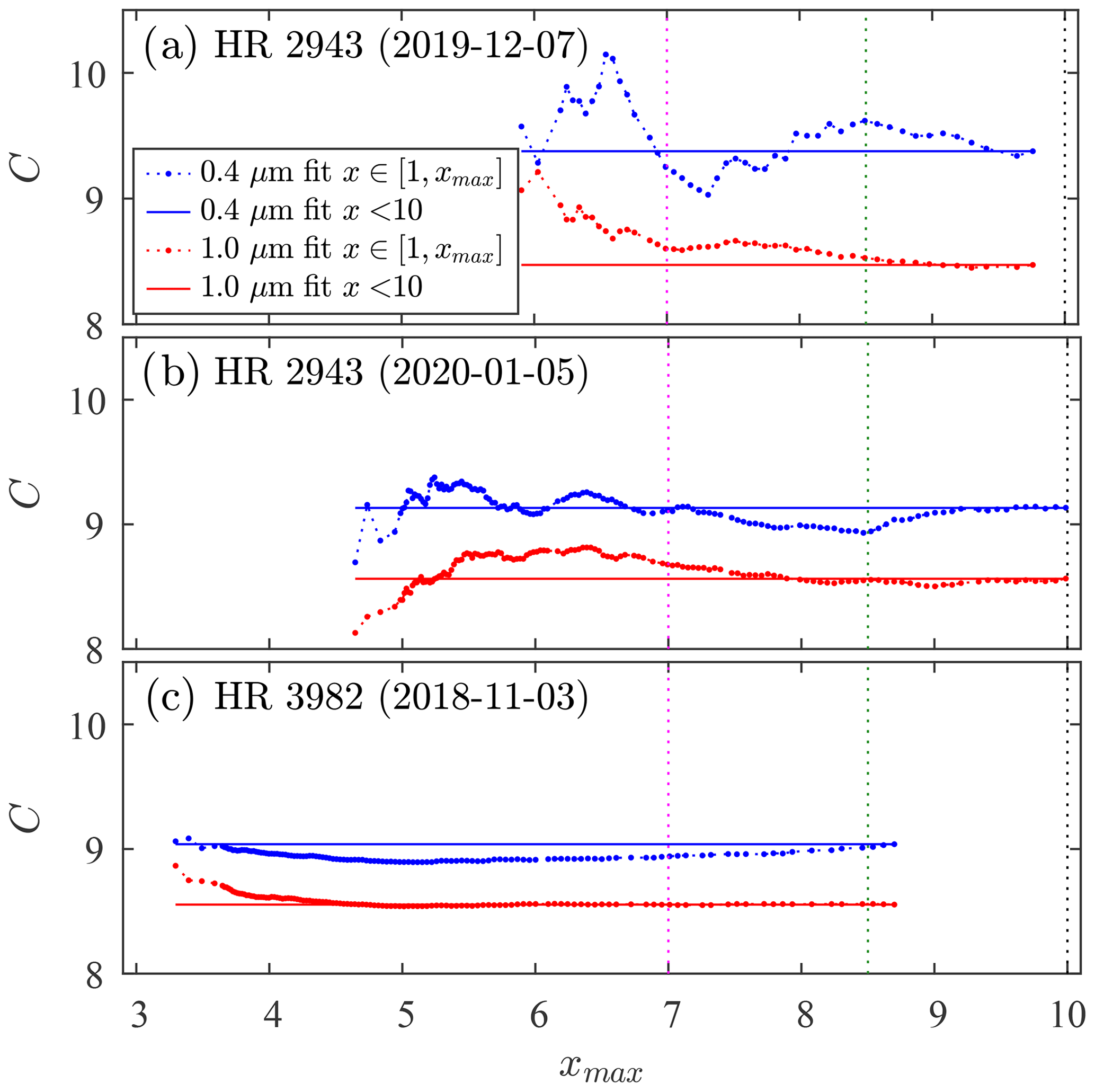
Figure 9C values retrieved from linear regressions over an increasing x range, i.e. from the smallest x to an increasing xmax for all the cases plotted in Fig. 8. The horizontal reference lines represent regressions over the entire x range (the solid lines of Fig. 8), while the three coloured (dotted) vertical lines correspond to the colours of the three xmax cases of Fig. 10.
The corresponding slope-derived τp spectra are shown in Fig. 10 for three xmax cases (the three coloured spectra were derived for xmax values corresponding to the matching colours of the three vertical lines in Figs. 8 and 9). The x-dependent regression error dynamics are investigated in Appendix C. The next subsection describes potential competing causes of C variations and makes a link to τp errors9.
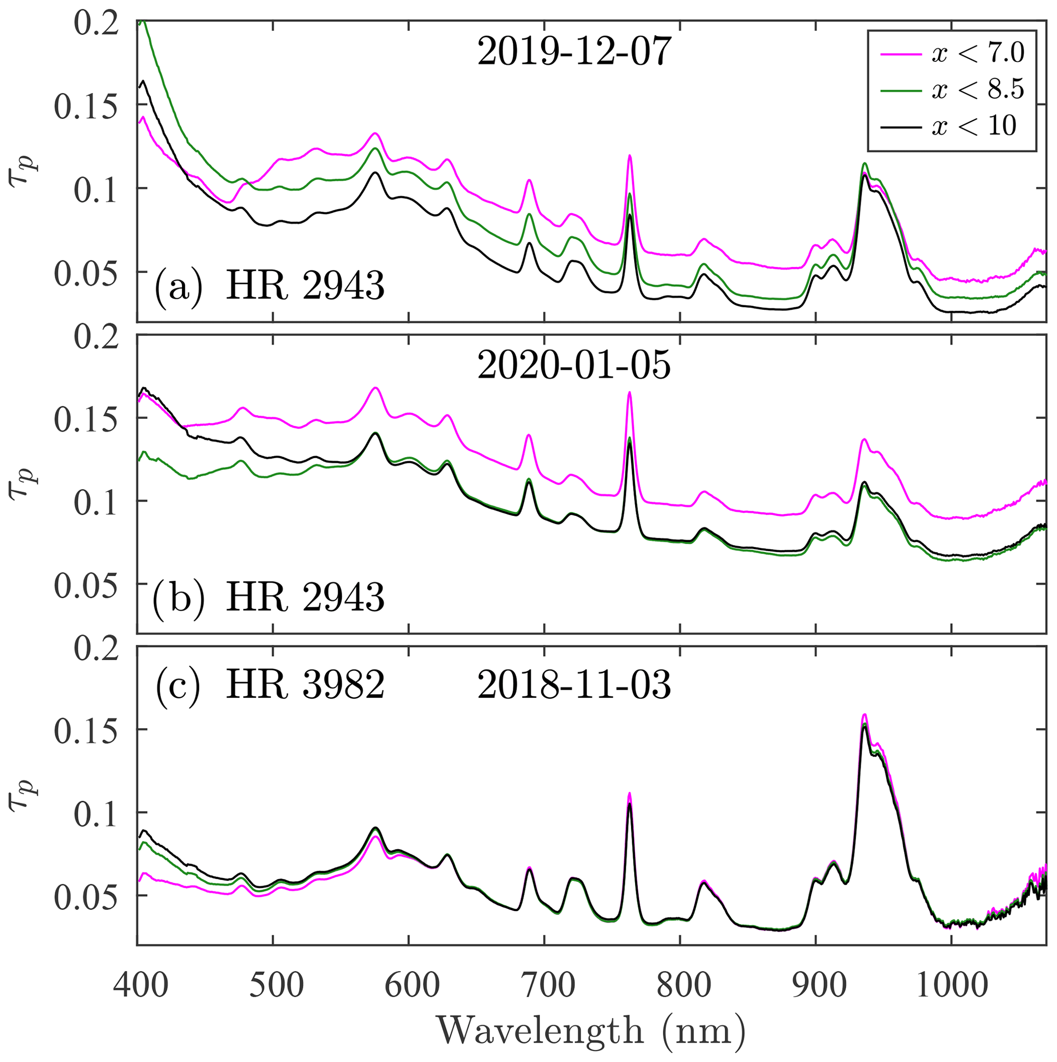
Figure 10Optical depth (slope) spectrum retrieved from calibration performed at different x ranges.
6.2 Regression error interpretation
The sky instability plots of Fig. 1 show that the standard deviation of the optical depth increases with time and air mass separation between any two stars (this applies equally well to the variation between two positions of the same star). A systematic optical depth drift during the calibration leads to a common-signed bias (positive or negative) of the regression slope and the calibration value, relative to drift-free conditions. Figure 10a and b show spectrum-wide τp reduction as xmax and calibration time increase. This suggests spatial and/or temporal sky transparency instability during calibration. Such rapid and spectrally neutral variation is consistent with the domination of coarse-mode (super µm) particles: a (post cloud-screened) mode that is mostly dominated by spatially homogeneous cloud particles at Eureka (O'Neill et al., 2016). The near-superposition of all τp spectra above 500 nm in Fig. 10c indicates stable transparency that is characteristic of a cloud-free atmosphere dominated by fine-mode (submicrometre) particles. A number-density-induced drift of similar fine-mode aerosol particles will generate spectrally independent variations in : the larger τp value (corresponding to the larger absolute difference in the blue/UV part of the spectrum) could explain the increasingly larger UV deviations (such as between the magenta and black/green curves in Fig. 10c).
The two bullet lists below summarize the specific processes that can lead to variations of calibration slope (τp) and intercept (C), traceable to real or apparent optical depth variations.
Instances of τp and C overestimation.
-
A systematic coarse-mode τp increase (as described above) can have a dramatic spectrum-wide effect: flagging and discarding such measurements is, accordingly, essential. A fine-mode τp increase will predominantly affect the UV/blue part of the spectrum.
-
Recent tests indicate that the optical collimation of the Eureka Celestron C11 telescope requires correction. Mis-collimation is responsible for a significant part of the star spot size reported in Ivănescu et al. (2021). Correcting the attendant vignetting problem (whose consequence is a decreased star flux and apparent increase in τp) may enable reliable measurements at x values well above the limit of x≃5 reported by Ivănescu et al. (2021).
-
The angular star spot size (ω), being proportional to (Eqs. 4.24, 4.25 and 7.70” of Roddier, 1981), effectively leads to spectrally dependent vignetting (i.e. apparent τp and C increase) as a function of x: an increase in x from 7 to 9.5 would be equivalent to 20 % of ω increase for a spectral change from 400 to 1000 nm. This coupled spectral and air mass vignetting influence is consistent with Fig. C1 with the blue (0.4 µm) curve increasing at x≃7, while the increase of the red (1.0 µm) curve occurs only at x>9. This dynamic potentially dominates the large UV/blue errors seen in Figs. 7 and 10.
-
Noisier star spots, attributable to increased turbulence and scintillation at large x, may induce larger centring errors and exacerbate apparent increases in τp and C due to vignetting.
Instances of τp and C underestimation.
-
There is a systematic τp decrease during the calibration period (notably when the calibration starts at large τp).
-
Weak signals, usually at large x and notably for hot stars in the NIR, may lead to sensitivity loss due to ADC (analog to digital conversion) limitations and attendant slope and intercept (τp and C) reductions.
These factors contribute to Fig. 10 τp dynamics and likely relate to the one-star spectra shown in Fig. 7. A very similar spectrum is indeed observed in the case of one faint star at large air mass (Fig. 11). Such spectral dynamics, possibly dominated by the aforementioned spectral influence of vignetting, are also likely related to the similar M0 bias spectra shown in Figs. 4 and 11 of Ivănescu et al. (2021). The identification of the M0 bias source is of paramount importance, as it may guide strategical observation choices made to improve the accuracy of future star catalogues. The error envelopes about the M0 bias (quantified in Fig. 12) add an additional, roughly flat spectral component (in spectral regions other than those that are dominated by H-absorption bands).
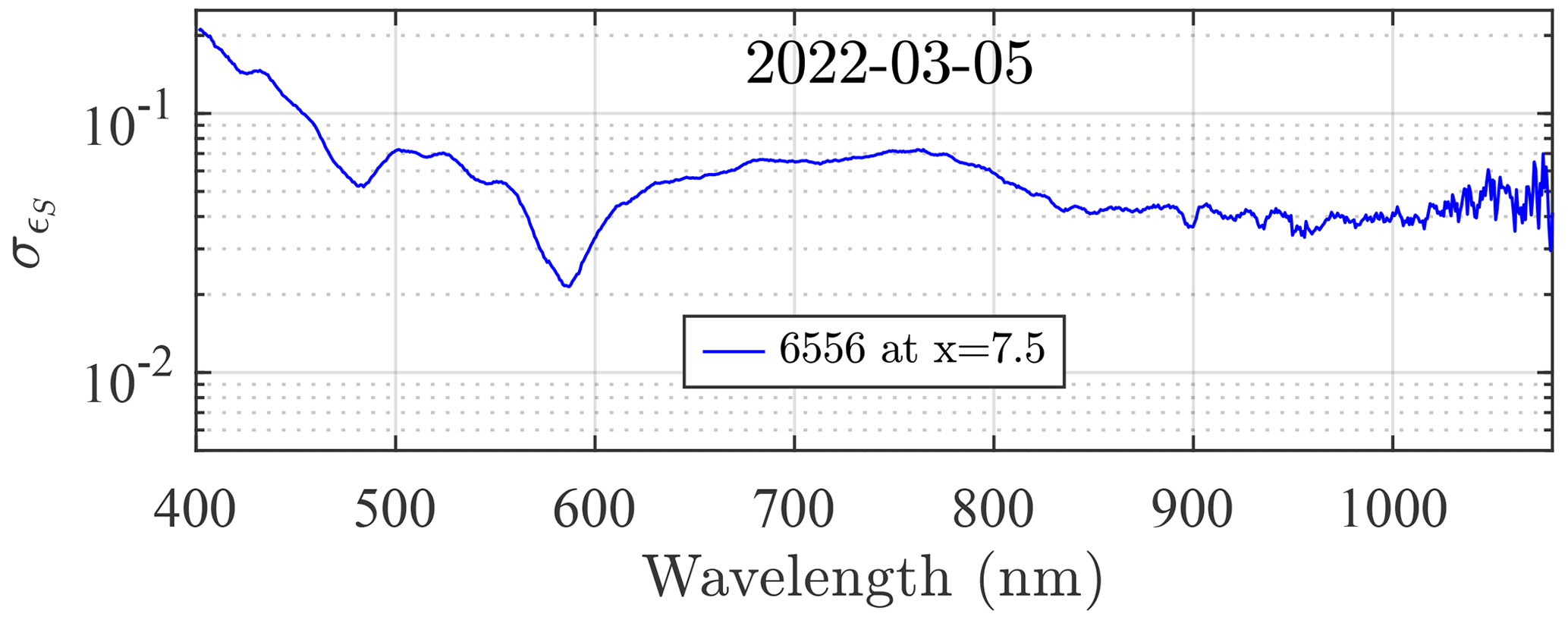
Figure 11Standard deviation of S magnitude measurements at large air mass for a faint catalogue star (HR 6556, V=2.08).
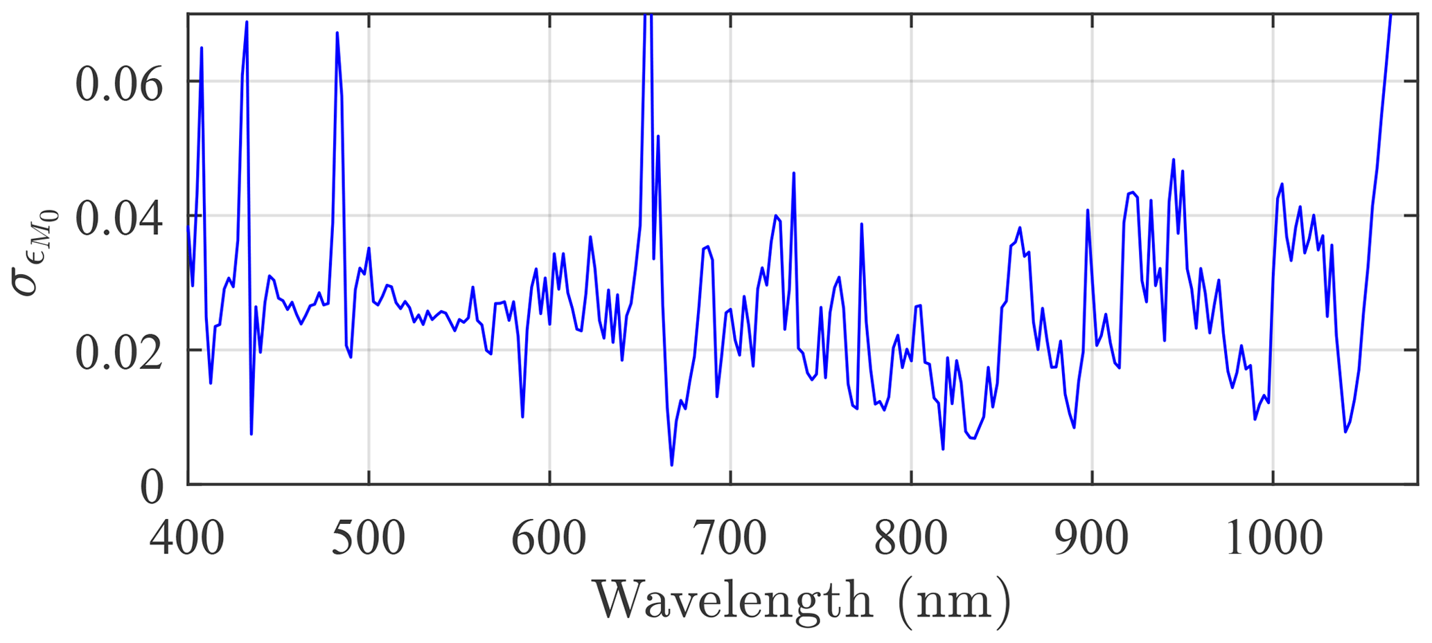
Figure 12Standard deviation of M0 errors deduced from the error bars of Fig. 4 in Ivănescu et al. (2021).
The smoother NIR errors in the one-star case (comparing the black one-star curve with the red multi-star curve of Fig. 5a for λ>1050 nm) are likely due to the strong NIR signal of the much colder Procyon star. One can take advantage of this effect and develop an observing strategy that avoids using faint stars at large air mass in Eureka and still employ 12 catalogue stars at x<8 in a multi-star calibration lasting 2.5 h (see Fig. A2). The star selection operation for a given multi-star calibration should also include a random air mass selection to mitigate accuracy errors attributable to systematic optical depth variations (as an alternative to the Rufener, 1986, method). Mitigation of both starlight reduction impacts at large air mass and systematic optical depth variations is a singular advantage of the multi-star vs. one-star calibration.
It was determined that no Eureka star movement satisfied an optimal sky-transit scenario of maximum possible air mass range within the constraint of x<5. The solution to this intrinsic shortcoming of a High Arctic site is to perform multi-star calibrations: this approach incorporates the fundamental advantage of reducing the calibration period and thus minimizing optical depth variability. It is, by its very nature, a calibration that enables the retrieval of a star-independent calibration parameter.
Multi-star calibration repeatability errors () were systematically smaller than the single-star errors and, in the central part of the spectrum, approached the target value of 0.01 for an observing period of 2.5 h. Those errors were partly affected by less than optimal clear-sky conditions (notably in the presence of cloud), with τp slightly larger than the recommended “clear-sky” value of 0.13: see Sect. 4 and Appendix A). Coarse-mode filtering algorithms, that ideally eliminate all influences of coarse-mode optical depth specifically in a calibration scenario, are necessary to ensure the best calibration10. Large UV and NIR errors can be reduced by avoiding faint stars at large x and by improving the current telescope collimation. The mitigation of mis-collimation problems can, in the short term, be affected by a constraint of x<7. This can be achieved at Eureka by employing 12 constrained-magnitude stars over a 3 h calibration period (see Appendix A). A constraint of τp<0.13 may bring the calibration errors in the blue-to-red spectral range closer to the 0.01 target, with the remaining UV and NIR spectral regions being subject to the influence of M0 errors.
In summary, the advantages of multi-star versus one-star calibration are star-independent calibration, faster coverage of larger air mass ranges, more calibration opportunities, and star selection capability for both mitigating the impact of starlight reduction with increasing air mass and systematic optical depth variations. These singular benefits were shown to override the drawbacks of specific star catalogue errors (i.e. the multi-star calibration performs better than the one-star case, even if the former is uniquely affected by M0 errors). Further improvement will only be achieved by developing a more accurate extraterrestrial star-magnitude catalogue: their UV/blue errors, likely linked to large-x spectral vignetting or fine-mode aerosol variations, are endemic to current ground-based star catalogues. This improvement may be affected from a space-borne platform or at a high-elevation observatory (the primary goal being to reduce turbulence-induced star-spot size and optical depth variability). The use of a large aperture telescope (limiting scintillation and low-starlight measurement errors) and a larger FOV instrument (less prone to vignetting) will, in general, provide better results.
Figure A1a shows the τp histogram for data acquired during the 2019–2020 observing season at Eureka11. The blue and red vertical lines respectively indicate the clear-sky cutoff values of 0.13 and 0.15 determined in Sect. 4 for the 2 h and 8 h calibrations. Operational conditions occurred 37 % of the time (i.e. those periods of time when measurements were not impeded by persistent thick clouds or the performance of maintenance tasks). A frequency curve of clear-sky periods (a period for which all τp values are less than the cutoff value) is presented in Fig. A1b. Measurements acquired during 2 h and 8 h clear-sky periods represented, respectively, 35.5 % and 39 % of all measurements. These numbers, transformed into an estimation of clear-sky fraction of the total measurement time, yield values of 13 % and 14 % of the total contiguous seasonal time (0.37⋅0.355 and 0.37⋅0.39, respectively). Since the measurement season is ∼160 d (or ∼5.3 months12) and given that there were 246 clear-sky periods of 2 h with τp<0.13, one may expect 46 such calibration periods per month. There were, on the other hand, 29 clear-sky periods of 8 h with τp<0.15 (or ∼5.5 per month). If a calibration can be successfully completed in ∼2 h, then there is a significantly larger probability-of-occurrence incentive for doing so.
The weakening of star signals with increasing air mass will progressively impact calibration quality. Figure A2 shows the availability of catalogue stars for a multi-star calibration over Eureka as a function of calibration period and maximum air mass. A calibration can, for example, be carried out in 2 h with only 11 stars of our 13-star dataset (Fig. 3). A 12-star calibration can be carried out only if x<9.5 or if the calibration period is >2.5 h.
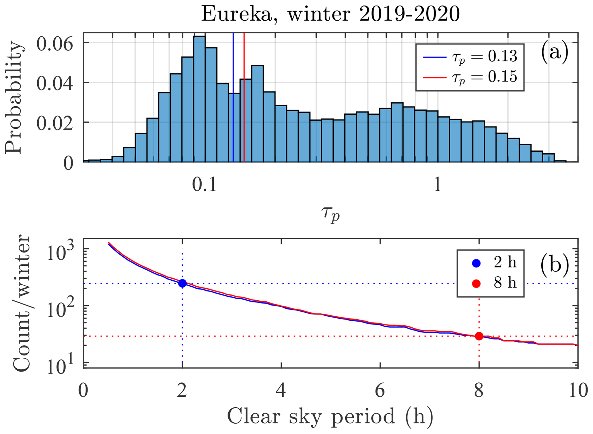
Figure A1τp histogram for measurements acquired during the 2019–2020 observing season at Eureka (total of 25914 measurements). The blue and red vertical lines are the clear-sky cutoff values of 0.13 and 0.15 determined in Sect. 4. The probability is normalized so that its sum is unity (a). Frequency of occurrence vs. duration of clear-sky periods (b).
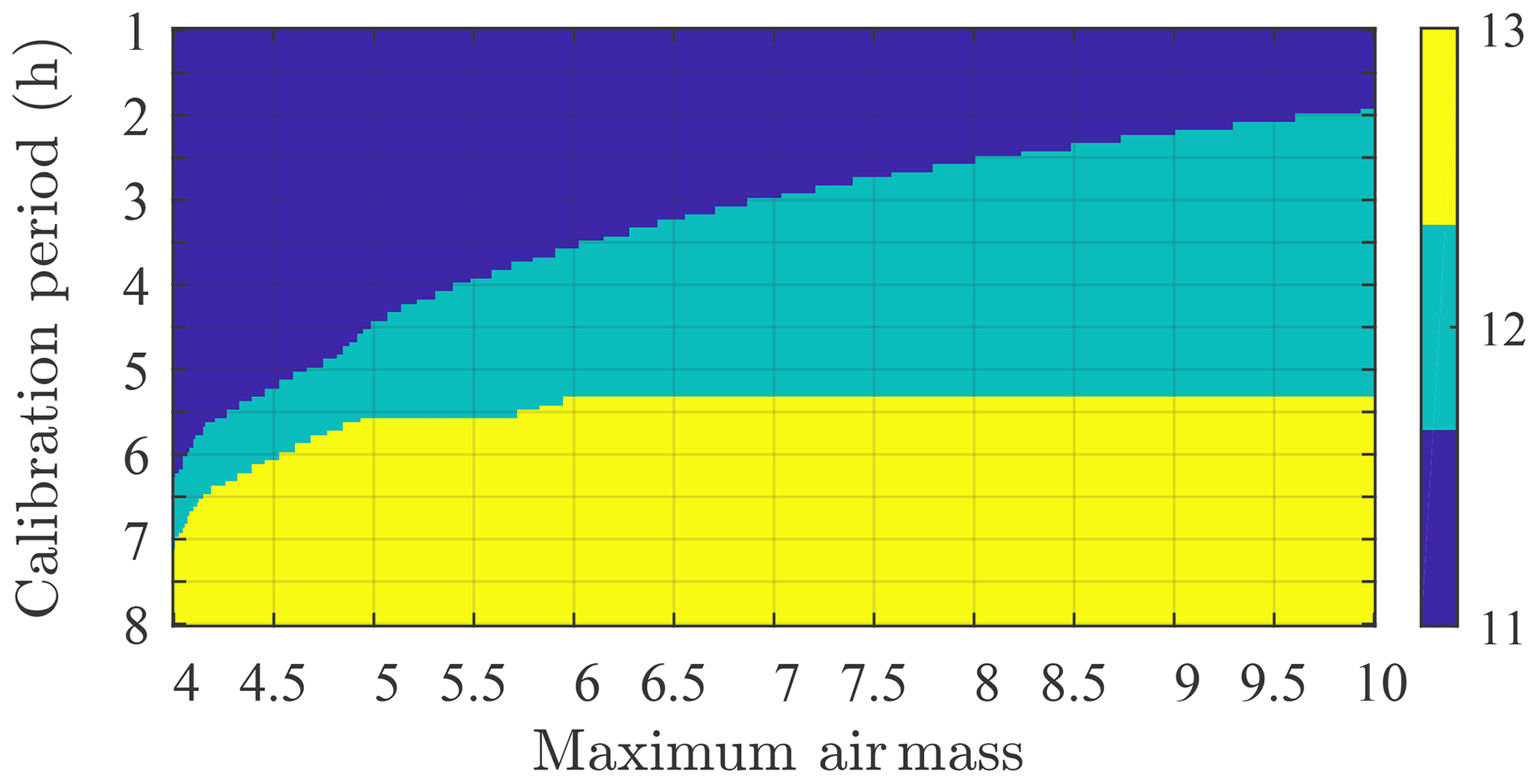
Figure A2Number of available catalogue stars for a multi-star calibration, during a 24 h period. The following constraints were employed in generating the tri-colour contours: at least one star at x<1.2 and exclusion of any star of visual magnitude V>1.5 for x>6, as well as V>2 at x>5.
From Eqs. (7) and (8) one gets the error propagation into the τ Langley retrieval:
Error propagation into the calibration constant (C) retrieval is, in a similar fashion, expressed as
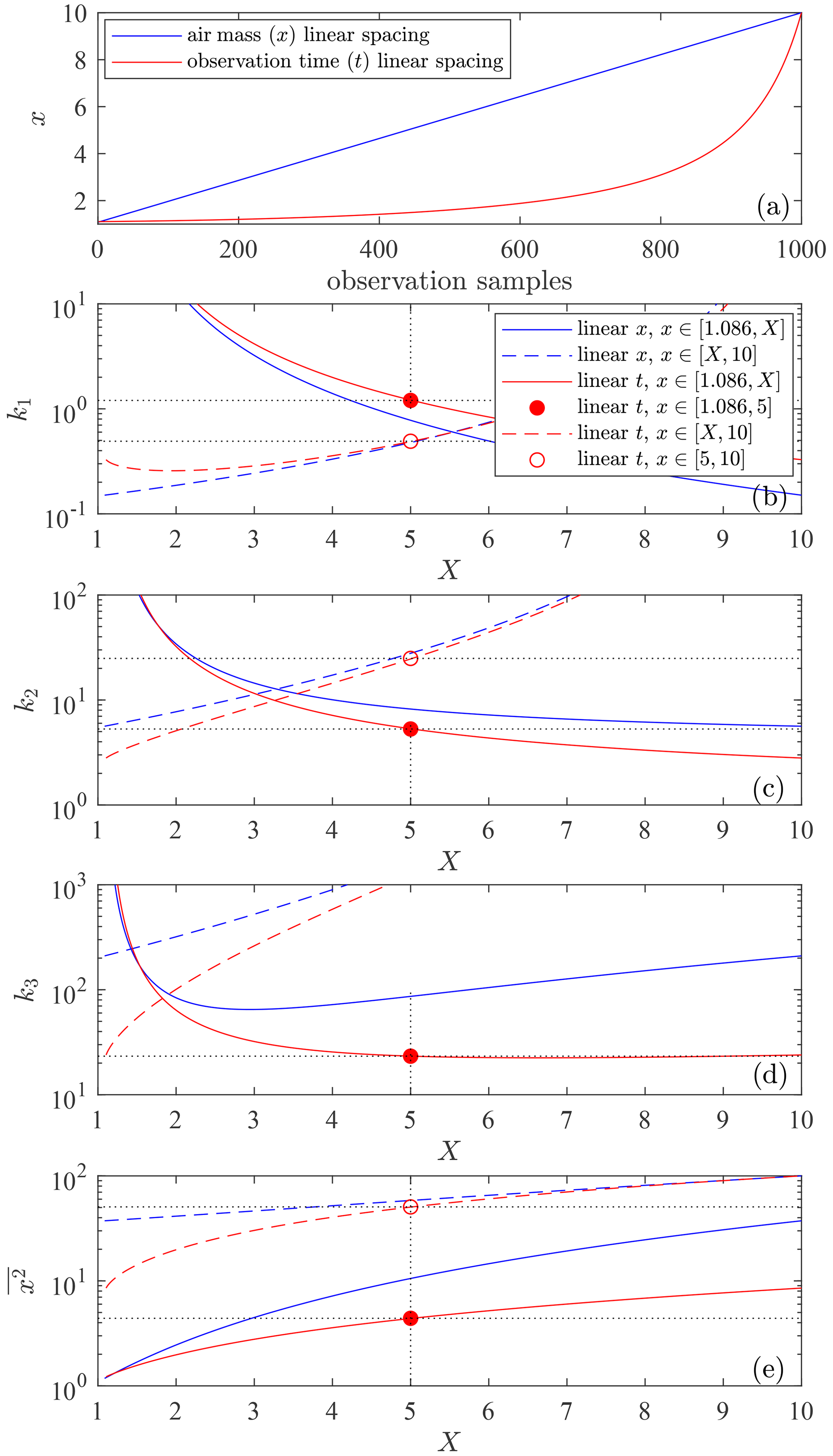
Figure B1Variation of x as a function of the number of observation samples for measurements made in equal increments of x (blue curve) and equal increments of time (red curve) (a). The next three panels show the x-dependent variation of k1, k2 and k3 (see text for more details). The legend in panel (b) applies to all the subsequent panels. Panel (e) shows , the to conversion factor of Eq. (B3).
The coefficients k1, k2 and k3 are displayed in Fig. B1b–d, respectively, for the x protocols of Fig. B1a. The blue curve shows uniformly distributed values of x, while the red curve shows a more realistic observing configuration of constant time intervals13. In order to investigate more practical (smaller) ranges, the working range is incrementally truncated from both the right and left (the solid and dashed curves, respectively). A particular focus is placed on two x ranges: the solid red circles for which x<5, where k1≃1.2, k2≃5.3 and k3≃23 (the k3 red curve flattens out for X>5 in Fig. B1d), and the open red circles for which x>5, where k1≃0.5, k2≃25 and k3≃1250 (k3 being 50 times the “x<5” value). This strong large-x weighting drives the standard error in C. (the zenith value of ) is typically ∼ στ, and thus ∼ (Ivănescu et al., 2021). Since ϵS depends on x14, 15∼ , both first terms of Eq. (B4) being driven by k3, which flattens out for , with X>5. They will generally tend then to dominate (unless N≪n), and thus the calibration error, particularly for large x ranges.
The C values, derived from tangents applied to the Fig. 8 solid curves (the means of a Δx=1.5 sliding window), are plotted in Fig. C1. The objective of this plot is to highlight more robust (lower frequency) C variations (and thus C errors) as a function of x. The 400 nm C values are relatively stable up to x≃7 to 7.5 where they are subject to a large increase. The 1000 nm C pattern is similar with an increase beginning at ≃9 (observations that are roughly consistent with the vignetting arguments of Sect. 6.2).
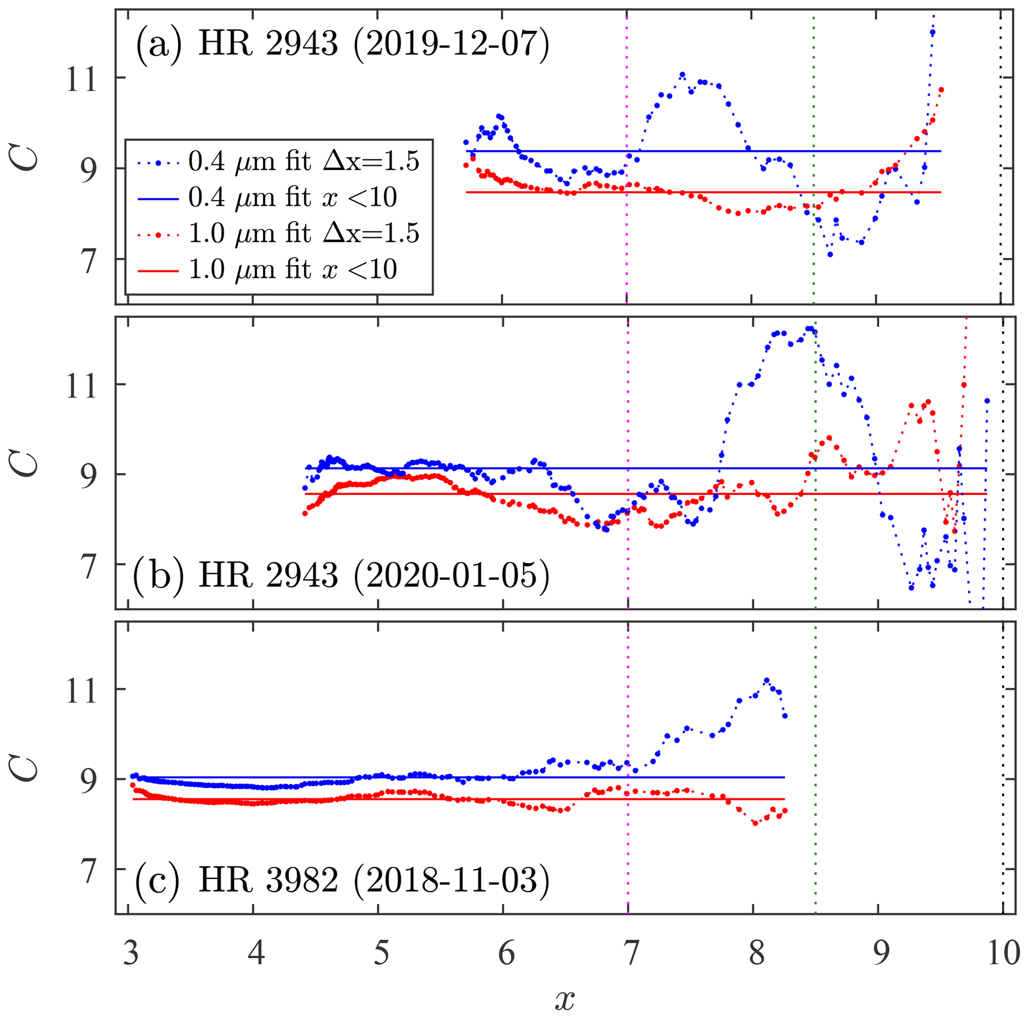
Figure C1The variable curves show the calibration (C) variation for regressions associated with the low-frequency (sliding window) curves of Fig. 8. The horizontal lines correspond to the single C value retrieved from the full (pan-x) regression lines of Fig. 8, while the three coloured (dotted) vertical lines correspond to the colours of the three xmax cases of Fig. 10.
Final MATLAB code and data employed in the generation of the figures are freely available (see https://doi.org/10.5281/zenodo.7975245, Ivănescu, 2023).
LI: conceptualization, methodology, data curation, software, formal analysis, investigation, writing original draft. NTO'N: validation, writing, review and editing, supervision, funding acquisition.
The contact author has declared that neither of the authors has any competing interests.
Publisher's note: Copernicus Publications remains neutral with regard to jurisdictional claims made in the text, published maps, institutional affiliations, or any other geographical representation in this paper. While Copernicus Publications makes every effort to include appropriate place names, the final responsibility lies with the authors.
This work was supported by CANDAC (the Canadian Network for the Detection of Atmospheric Change) via the NSERC PAHA (Probing the Atmosphere of the High Arctic) project, by the NSERC CREATE Training programme in Arctic Atmospheric Science and by the Canadian Space Agency (CSA). Finally we also gratefully acknowledge the support of the CANDAC operations staff at Eureka for their numerous troubleshooting interventions.
This research has been supported by the Natural Sciences and Engineering Research Council of Canada (NSERC; grant nos. RGPCC-433842-2012 and CREATE 384996-10) and by the Canadian Space Agency (CSA; grant nos. 21SUASACOA and 00353/15FASTA12).
This paper was edited by Daniel Perez-Ramirez and reviewed by two anonymous referees.
Alekseeva, G. A., Arkharov, A. A., Galkin, V. D., Hagen-Thorn, E., Nikanorova, I., Novikov, V. V., Novopashenny, V., Pakhomov, V., Ruban, E., and Shchegolev, D.: The Pulkovo Spectrophotometric Catalog of Bright Stars in the Range from 320 TO 1080 NM, Balt. Astron., 5, 603–838, https://doi.org/10.1515/astro-1997-0311, 1996. a
Baibakov, K., O'Neill, N. T., Ivanescu, L., Duck, T. J., Perro, C., Herber, A., Schulz, K.-H., and Schrems, O.: Synchronous polar winter starphotometry and lidar measurements at a High Arctic station, Atmos. Meas. Tech., 8, 3789–3809, https://doi.org/10.5194/amt-8-3789-2015, 2015. a
Barford, N.: Experimental measurements: precision, error and truth, 2nd edn., John Wiley and Sons Ltd., Chichester, https://www.worldcat.org/oclc/11622295 (last access: 4 December 2023), 1985. a
Dachs, J.: Lichtelektrische Sternphotometrie und Farbenindexmessungen durch Zählung von Photoelektronen, PhD thesis, Tübingen University, https://www.worldcat.org/title/249623335 (last access: 4 December 2023), 1960. a
Dachs, J.: Ein Photoelektronen zählendes Sternphotometer, Astron. Nachr., 289, 129–138, https://doi.org/10.1002/asna.19662890305, 1966. a
Dachs, J., Haug, U., and Pfleiderer, J.: Atmospheric extinction measurements by photoelectric star photometry, J. Atmos. Terr. Phys., 28, 637–649, https://doi.org/10.1016/0021-9169(66)90077-8, 1966. a
Goodman, L. A.: On the Exact Variance of Products, J. Am. Stat. Assoc., 55, 708–713, https://doi.org/10.1080/01621459.1960.10483369, 1960. a
Gröschke, A., Herber, A. B., Schrems, O., Schulz, K.-H., and Gundermann, J.: Development and application of a new star photometer for measuring aerosol optical depth at harsh environments, in: EGU General Assembly 2009, 19–24 April 2009, Vienna, Austria, 10485, https://meetingorganizer.copernicus.org/EGU2009/EGU2009-10485.pdf (last access: 4 December 2023), 2009. a
Ivănescu, L.: Une application de la photométrie stellaire à l'observation de nuages optiquement minces à Eureka, NU, Master in science thesis, UQAM, http://www.archipel.uqam.ca/id/eprint/8417 (last access: 4 December 2023), 2015. a
Ivănescu, L.: Multi-star calibration in starphotometry, code and data, Zenodo [data set], https://doi.org/10.5281/zenodo.7975245, 2023. a
Ivănescu, L., Baibakov, K., O'Neill, N. T., Blanchet, J.-P., and Schulz, K.-H.: Accuracy in starphotometry, Atmos. Meas. Tech., 14, 6561–6599, https://doi.org/10.5194/amt-14-6561-2021, 2021. a, b, c, d, e, f, g, h, i, j, k, l, m, n
Montgomery, D. C. and Runger, G. C.: Applied Statistics and Probability for Engineers, 5th edn., John Wiley and Sons, Inc., http://www.worldcat.org/oclc/28632932 (last access: 4 December 2023), 2011. a
Oh, Y.-L.: Retrieval of Nighttime Aerosol Optical Thickness from Star Photometry, Atmosphere, 25, 521–528, https://doi.org/10.14191/Atmos.2015.25.3.521, 2015. a
O'Neill, N. T., Baibakov, K., Hesaraki, S., Ivanescu, L., Martin, R. V., Perro, C., Chaubey, J. P., Herber, A., and Duck, T. J.: Temporal and spectral cloud screening of polar winter aerosol optical depth (AOD): impact of homogeneous and inhomogeneous clouds and crystal layers on climatological-scale AODs, Atmos. Chem. Phys., 16, 12753–12765, https://doi.org/10.5194/acp-16-12753-2016, 2016. a, b, c
Pérez Ramírez, D.: Caracterización del aerosol atmosférico en la ciudad de Granada mediante fotometría solar y estelar, PhD thesis, Granada, http://hdl.handle.net/10481/5628 (last access: 4 December 2023), 2010. a
Pérez-Ramírez, D., Aceituno, J., Ruiz, B., Olmo, F. J., and Alados-Arboledas, L.: Development and calibration of a star photometer to measure the aerosol optical depth: Smoke observations at a high mountain site, Atmos. Environ., 42, 2733–2738, https://doi.org/10.1016/j.atmosenv.2007.06.009, 2008. a
Pérez-Ramírez, D., Lyamani, H., Olmo, F. J., and Alados-Arboledas, L.: Improvements in star photometry for aerosol characterizations, J. Aerosol Sci., 42, 737–745, https://doi.org/10.1016/j.jaerosci.2011.06.010, 2011. a
Pérez-Ramírez, D., Navas-Guzmán, F., Lyamani, H., Fernández-Gálvez, J., Olmo, F. J., and Alados-Arboledas, L.: Retrievals of precipitable water vapor using star photometry: Assessment with Raman lidar and link to sun photometry, J. Geophys. Res.-Atmos., 117, D05202, https://doi.org/10.1029/2011JD016450, 2012. a
Roddier, F.: The Effects of Atmospheric Turbulence in Optical Astronomy, in: Progress in Optics, chap. V, Elsevier, 281–376, https://doi.org/10.1016/S0079-6638(08)70204-X, 1981. a
Rousseeuw, P. J. and Croux, C.: Alternatives to the Median Absolute Deviation, J. Am. Stat. Assoc., 88, 1273–1283, https://doi.org/10.1080/01621459.1993.10476408, 1993. a
Rufener, F.: Technique et réduction des mesures dans un nouveau système de photométrie stellaire, Publications de l'Observatoire de Genève, Série A: Astronomie, chronométrie, géophysique, 66, 413–464, http://www.worldcat.org/oclc/491819702 (last access: 4 December 2023), 1964. a
Rufener, F.: The evolution of atmospheric extinction at La Silla, Astron. Astrophys., 165, 275–286, http://adsabs.harvard.edu/abs/1986A&A...165..275R (lsat access: 4 December 2023), 1986. a, b
Sayer, A. M. and Knobelspiesse, K. D.: How should we aggregate data? Methods accounting for the numerical distributions, with an assessment of aerosol optical depth, Atmos. Chem. Phys., 19, 15023–15048, https://doi.org/10.5194/acp-19-15023-2019, 2019. a
Soch, J., Faulkenberry, T. J., Petrykowski, K., Allefeld, C., and McInerney, C. D.: The Book of Statistical Proofs, Open, Zenodo, https://doi.org/10.5281/zenodo.5820411, 2021. a
Théorêt, X.: AEROSTAR Conception d'un spectroradiomètre stellaire pour l'étude des aérosols noctures, PhD thesis, Sherbrooke, http://savoirs.usherbrooke.ca/handle/11143/2335 (last access: 4 December 2023), 2003. a
Young, A. T.: Observational Technique and Data Reduction, in: Methods in Experimental Physics, vol. 12, chap. 3, Elsevier, 123–192, https://doi.org/10.1016/S0076-695X(08)60495-0, 1974. a
Made by Dr. Schulz & Partner GmbH (currently closed).
Such an error becomes part of the C value extracted from the Langley calibration of Eq. (4) and becomes part of the operational retrieval process when Eq. (4) is inverted to yield individual values of τ.
n>10, where (ni being the number of observations associated with star i).
A cutoff liberty that we availed ourselves of because one is free to choose the duration of the calibration period and/or to perform outlier filtering prior to Langley regressions.
Using (obtained from Eq. B3), with the terms in S and M0 neglected, and inserting (i.e. ) into Eq. (7) and noting that a typical range of yields k3≃23 (see Fig. B1).
The other bright stars, being of similar A–B type (Ivănescu et al., 2021), exhibit lower signal-to-noise ratios (SNRs) in the NIR.
Standard deviations that, we would argue, are also standard errors (each of the three spectra that were averaged were more akin to means).
The strong, positive correlation between C and τp and between their errors is the result of variations in the regression lines being effectively driven by rotations about a cluster of pivot points whose x position changes little.
Clouds are usually the dominant coarse-mode component, but coarse-mode aerosols can have diverse effects, which are typically, but not always, minor.
We could speculate that the two histogram peaks near τp values of 0.1 and 0.16 are associated with the background fine-mode optical depth and the enhanced fine-mode optical depth incited by the presence of wind-blown sea salt (O'Neill et al., 2016).
Which we pragmatically define as the number of nights for which reliable measurements can be carried out for ≥30 min.
Both conditions apply to a star crossing the meridian at zenith.
- Abstract
- Introduction
- Calibration methodology
- Calibration errors
- Observing conditions
- Multi-star calibration
- Regression error discussion
- Conclusions
- Appendix A: Calibration opportunities
- Appendix B: Relative importance of component errors
- Appendix C: Error discussion supplement
- Code and data availability
- Author contributions
- Competing interests
- Disclaimer
- Acknowledgements
- Financial support
- Review statement
- References