the Creative Commons Attribution 4.0 License.
the Creative Commons Attribution 4.0 License.
 | 14 Feb 2023
Toward quantifying turbulent vertical airflow and sensible heat flux in tall forest canopies using fiber-optic distributed temperature sensing
Mohammad Abdoli
Karl Lapo
Johann Schneider
Johannes Olesch
Christoph K. Thomas
The paper presents a set of fiber-optic distributed temperature sensing (FODS) experiments to expand the existing microstructure approach for horizontal turbulent wind direction by adding measurements of turbulent vertical component, as well as turbulent sensible heat flux. We address the observational challenge to isolate and quantify the weaker vertical turbulent motions from the much stronger mean advective horizontal flow signals. In the first part of this study, we test the ability of a cylindrical shroud to reduce the horizontal wind speed while keeping the vertical wind speed unaltered. A white shroud with a rigid support structure and 0.6 m diameter was identified as the most promising setup in which the correlation of flow properties between shrouded and reference systems is maximized. The optimum shroud setup reduces the horizontal wind standard deviation by 35 %, has a coefficient of determination of 0.972 for vertical wind standard deviations, and a RMSE of less than 0.018 ms−1 when compared to the reference. Spectral analysis showed a fixed ratio of spectral energy reduction in the low frequencies, e.g., <0.5 Hz, for temperature and wind components, momentum, and sensible heat flux. Unlike low frequencies, the ratios decrease exponentially in the high frequencies, which means the shroud dampens the high-frequency eddies with a timescale <6 s, considering both spectra and cospectra together. In the second part, the optimum shroud configuration was installed around a heated fiber-optic cable with attached microstructures in a forest to validate our findings. While this setup failed to isolate the magnitude and sign of the vertical wind perturbations from FODS in the shrouded portion, concurrent observations from an unshrouded part of the FODS sensor in the weak-wind subcanopy of the forest (12–17 m above ground level) yielded physically meaningful measurements of the vertical motions associated with coherent structures. These organized turbulent motions have distinct sweep and ejection phases. These strong flow signals allow for detecting the turbulent vertical airflow at least 60 % of the time and 71 % when conditional sampling was applied. Comparison of the vertical wind perturbations against those from sonic anemometry yielded correlation coefficients of 0.35 and 0.36, which increased to 0.53 and 0.62 for conditional sampling. This setup enabled computation of eddy covariance-based direct sensible heat flux estimates solely from FODS, which are reported here as a methodological and computational novelty. Comparing them against those from eddy covariance using sonic anemometry yielded an encouraging agreement in both magnitude and temporal variability for selected periods.
- Article
(8987 KB) - Full-text XML
-
Supplement
(441 KB) - BibTeX
- EndNote


Most fluids at sufficiently high Reynolds numbers feature general flow patterns combined with random motions called “turbulence” (Corrsin, 1961). From a micrometeorological point of view, turbulence is the primary mechanism for mixing energy and matter in the air, and its strength controls the coupling between the atmosphere and the earth surface (Burgers, 1948; Tennekes et al., 1972). Understanding the nature of turbulent flow is essential for many applications, such as the transfer and mixing of light, heat, water vapor, carbon dioxide, nutrients, and other substances, directly affecting humans, animals, and plants' quality of life. Although current theories describe the transport and turbulent mixing near the surface for sufficiently strong winds well (Van de Wiel et al., 2012), under stable regimes, the atmospheric boundary layer (ABL) turbulence does not obey well-known concepts, including the Monin–Obukhov similarity theory, the Kolmogorov spectrum, and Taylor's hypothesis of frozen turbulence (Sun et al., 2012; Grachev et al., 2013; Cheng et al., 2017).
For weak-wind conditions, turbulence is not exclusively governed by dynamic stability but is driven by a combination of non-stationary processes, sub-mesoscale motions, local shear, and flow instabilities (Sun et al., 2012; Mahrt et al., 2013; Liang et al., 2014). Intermittent turbulence or non-stationary conditions often violate assumptions made for scaling laws and statistical approaches used in micrometeorology, including translation of temporal scales into length scales through applying the assumption of Taylor's frozen turbulence. Also, the ergodicity assumption cannot be applied to the single-point measurements in these conditions. The ergodicity assumption states that the time and space averages converge under stationary, horizontally homogeneous conditions (Engelmann and Bernhofer, 2016). Several efforts have been made to analyze observations from networks of sensors to elucidate intermittent processes such as meandering and within-canopy flow and heat transport (Anfossi et al., 2005; Thomas, 2011). Despite some progress in the mentioned studies, the lack of spatial information sufficiently dense to resolve the process scales has hindered advancing the stable boundary layer's current physical interpretation.
Fiber-optic distributed temperature sensing (FODS) has been introduced as a powerful geophysical technique in the last few years. This technique measures the temperature along a fiber-optic cable at a time resolution of a few seconds and spatial resolution of tens of centimeters up to 20 km in total length (Thomas and Selker, 2021). It is capable of observing atmospheric flows under physically poorly understood sub-meso motions (Thomas et al., 2012; Pfister et al., 2021). The distributed temperature sensing (DTS) technique's utility in atmospheric measurement is not limited to measuring the distributed temperature of the air, water, ice, snow, soil, and plant, but various applications such as measurement of evapotranspiration, soil moisture, humidity, shortwave radiation, and wind speed have been tested successfully (Predosa, 2016; Schilperoort et al., 2020; Thomas and Selker, 2021).
Among the most recent development of this technique, Lapo et al. (2020) introduced an approach using an FO cable with a cone-shaped microstructure printed on it, which causes directional differences in the convective heat loss from the FO cable to the air. When heated coned fibers are placed in the main flow direction, the fibers on which the cones are aligned with the flow cool more than those with opposing alignment, enabling computation of wind direction. The before-mentioned study was conducted in idealized wind tunnel experiments. Very recently, Freundorfer et al. (2021) deployed this approach for the first time during actual field observation. They presented three different methods of calculating turbulent horizontal wind directions from the FODS measurements, indicating the potential of this approach to reveal the wind direction's spatial structures at scales of meters and tens of seconds. The last two studies aimed at building a fully three-dimensional, spatially resolving atmospheric flow sensor as an important step toward a spatially distributed flux sensor using the eddy covariance technique. Although measuring the horizontal wind component was successful, the vertical wind component could not be measured with existing approaches to complete the three-dimensional sensor functionality to date. Measuring the vertical wind component with the heated coned fiber approach is challenging as (i) the magnitude of the vertical wind fluctuations is smaller than the combined signals of horizontal mean and turbulent flows, and (ii) the duration of the vertical events are too short, which leads to vanishing sensitivity in the vertical direction because of the finite response time of the FODS sensor. Isolating the vertical wind signal by filtering the horizontal wind is essential to capture the signals induced by the air's vertical movement. Having truly three-dimensional spatially resolved observations would create a possibility to compute the momentum and sensible heat fluxes independently of the fundamental assumptions of ergodicity, stationarity, and homogeneity, since the observations are taken simultaneously in both time and space domains. For example, it could be used to reveal the generating mechanism of the weak and intermittent turbulence where the conventional observation assumptions fail. A three-dimensional spatially resolved observation could also explain the long-standing problem of counter-gradient flux caused by a poor choice of height in the measurement and perturbation timescale (Vickers and Thomas, 2014; Fritz et al., 2021).
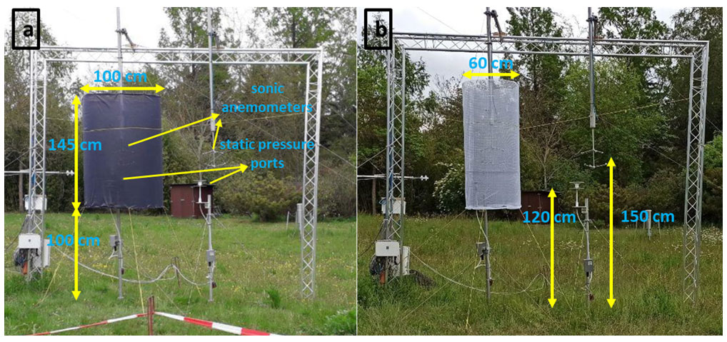
Figure 1Two examples of a shroud experiment setup containing two upside-down sonic anemometers and two high-precision pressure transducers with the quad disk to measure static pressure. (a) A 1 m diameter cylindrical shroud with fine-porosity gray color texture. (b) A 60 cm cylindrical shroud with a white insect screen.
We aimed to overcome these conceptual and observational challenges by conducting a series of experiments. The first part of this study was conducted above an open grassland and used only classic sonic anemometry without FODS to identify an optimal experimental configuration for subsequent testing in the second part with the use of FODS. We diminished the horizontal wind speed using different cylindrical shrouds and compared the flow characteristics inside and outside the shroud by placing a sonic anemometer inside and outside the shroud to investigate (i) which are the optimal physical properties of the shroud (aspect ratio, shape, porosity, rigidity, and color) to diminish the horizontal wind disturbances adequately while leaving the vertical wind perturbations largely unaffected. And (ii) how is the spectra of turbulent fluctuations affected by shroud in high and low frequencies compared to an unshrouded setup? In the second part of this study, a forest environment was used to investigate the applicability of the fiber-optic approach to measuring vertical wind components. We considered forests an ideal test environment, since the mixing-layer-type flow characterized by coherent structures with strong vertical motions and the sweep and ejection phases in the subcanopy allow for sustained stronger vertical wind speed compared to horizontal wind speed (Brunet, 2020). We deployed a shroud based on the results of the first part around heated coned FO cables in the forest area to see (iii) whether vertical wind direction and wind speed can be resolved by affixing a shroud around actively heated coned FO cables and if this setup can be used to compute the sensible heat flux purely based on FODS. If yes, how is the quality of the derived component based on point measurement?
2.1 Part 1: shroud experiment over grassland
The first part of the measurements was conducted between April 2020 and June 2020 at the Ecological Botanical Garden (EBG) at the University of Bayreuth. The experimental area was covered with short grass (5–15 cm) surrounded by mixed types of trees with an approximate height of 15 m from north, northeast, and southeast and a small artificial pond on the west side. Based on the synoptic weather station data close to the experiment location from 2014 to 2018, the dominant wind direction for spring and summer is westerly and southwesterly, with a maximum wind speed of 8–12 ms−1. Two upside-down sonic anemometers (Model USA-1, METEK GmbH, Elmshorn, Germany) at a 1.5 m height (middle of the shroud) and two quad disk pressure ports attached to a nano-resolution digital barometer (Model 745-16B, Paroscientific, Inc.) at 1.2 m above ground were set up. One set of sensors was placed inside the cylindrical shroud (Fig. 1). The spacing between two sets of sensors was 1.5 m to reduce the potential airflow distortion of the shrouded setup on the unshrouded setup. White and gray insect screens with a mesh size of approximately 0.5 and 0.1 mm, respectively, are used. The supporting structures of the shroud and sonic anemometers are oriented along the north-west direction, perpendicular to dominant wind speed, to reduce the structure-induced systematic disturbances. A metal wire mesh with a 10 mm × 10 mm grid size is used underneath the shroud to enhance its rigidity against distortion during stronger winds.
We iterated multiple shroud configurations in different diameters (1 and 0.6 m), gray and white colors, small and large pore sizes, and with and without supporting the metal mesh underneath the shroud. The reasoning for each selection is as follows:
-
Diameter. The task was to design a shroud to eliminate the horizontal flow while keeping the vertical flow perturbation intact. We hypothesized increasing the shroud diameter could increase the horizontal flow disturbances inside the shroud, since it offers a larger pathway for airflow. On the other hand, decreasing the shroud diameter and placing it close to the sonic anemometer could cause systematic turbulence created with the shroud itself.
-
Length. We determined the length of the shroud over the grass to be long enough to accommodate the typical length scales of the vertical turbulent flow, keep the sensors away from shroud structure-induced flow disturbances, and be feasible to install, given the available hardware and facilities.
-
Color. We used the gray shroud first. Initial results showed substantial heating of the shroud material during daytime conditions, inducing strong upward-directed (free) convective heat transfer and thus distorting flow statistics inside the shroud. In response, we changed the shroud's color to white to avoid possible radiative heating errors, together with increasing the pore size of the shroud.
-
Mesh size. The initial mesh size was selected based on the previous experiments and then improved based on the initial results.
-
Rigidity. The very first setup of the shroud was designed without supporting mesh and was just a tensioned shroud with two rings at the top and bottom. We observed that the shroud became very unstable during wind gusts and induced uninvited turbulence. We decided to make the shroud rigid enough to avoid this problem.
The sonic anemometer and static pressure data recorded at sampling frequencies of 20 Hz and perturbation and averaging timescales of 10 min were used to compute sensible heat and momentum fluxes and compare wind components inside and outside the shroud. In this part of the study, no FODS techniques were used, and the primary objective was to determine the best configuration of the shroud to meet the study's objectives. Three sets of shroud experiments at EBG were compared in this study with setup 1 standing for a gray, dense 1 m diameter shroud, setup 2 for a gray, dense 60 cm diameter shroud, and setup 3 for a white, not dense 60 cm diameter shroud.
2.2 Part 2: shroud experiment in a forest
The second part of the study evaluated the utility of the shroud approach at the Waldstein–Weidenbrunnen long-term ecosystem flux site between October and November 2020 as part of the Large-eddy ObsErvatory Waldstein Experiment 2020 (LOEWE20) experiment. The Waldstein is a forested site in the Fichtelgebirge Mountains located within the Lehstenbach catchment. This forest was mainly covered by Norway spruce (Picea abies), characterized by variable tree heights and densities. Subcanopy vegetation is moderately dense with a cumulative plant area index of 0.7 m2 m−2, featuring shrubs with a height of ≤1 m. The plant area index (PAI) is 5.6±2.1 m2 m−2 for the overstory trees and 3.5 m2 m−2 for the understory trees. In the Waldstein site, westerly and southeasterly wind with a wind speed range of 2 to 5 ms−1 dominate in the overstory; in the subcanopy, it is northerly and southwesterly with a range of 1 to 2 ms−1 (Foken et al., 2017). The experiment period was mostly dominated by anticyclonic conditions in both 500 and 950 hPa isobaric levels, with southwesterly winds being partly wet and partly dry. The shroud was installed at the main tower around a quartet FO array containing two pairs of parallel coned and unconed FO cables extending from the ground to the top canopy at a 34 m height (Fig. 2). The center of the shroud was placed at 4 m above ground, having the same diameter as the first part of the study, but its lower boundary was located 2.75 m above ground. Two high-resolution DTS instruments (Model 5 km ULTIMA, Silixa, London, UK) were used to observe the continuous temperature with a spatial resolution of 0.127 m averaged over 3 s. The DTS device was connected to one of four 50 µm multimode bend-insensitive cores inside a high-resistance stainless steel sheath filled with gel (inner tube diameter = 1.06 mm, outer diameter = 1.32 mm; Model C-Tube, Solifos AG, Switzerland; resistance = 1.8Ω m−1). The cones are made from polyethylene with a diameter and height of 12 mm, spaced at 2 cm along the fiber-optic cable (Lapo et al., 2020). Two warm and cold solid-phase calibration baths with a constant temperature developed by Thomas et al. (2022) were deployed at the beginning and end of FO arrays to be used as a calibration reference (Fig. 2). A sensor package was set outside the shroud close to the center of the cylinder with a sonic anemometer (Model CSAT3, Campbell Scientific Inc., Logan, UT, USA), a quad disk static pressure transducer (Model 745-16B, Paroscientific, Inc.), and an open-path infrared CO2 H2O gas analyzer (Licor 7500, LI-COR Biosciences, USA). For comparison reasons, the eddy covariance data with a sampling frequency of 10 Hz at a 36 m height and the FODS data of quartet array from the turbulence tower located approximately 70 m away from the main tower were used. See Foken et al. (2021) for more details on the turbulence tower specification. The quartet fiber configuration at the turbulence tower is the same as the main tower extending from the ground to a 34 m height. It should be noted that all of the eddy covariance data in this study were sampled at 20 Hz, with the exception of the permanent eddy covariance station at the turbulence tower, which was sampled at 10 Hz. All of the eddy covariance systems in this study use the same eddy covariance data processing and flux computation routine described in Thomas et al. (2009; see Appendix A).
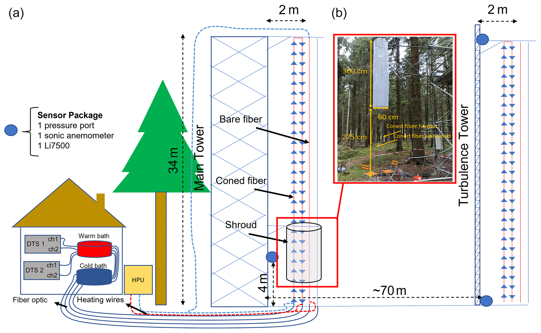
Figure 2(a) Shroud experiment schematic at Waldstein forest including a quartet of a vertical FO array and affixing a shroud at a 4 m height at the main tower close to the sensor package, including a static pressure port, a sonic anemometer, and an open-path infrared gas analyzer. Each coned and unconed fiber is connected to separate DTS devices. For DTS data calibration purposes, warm and cold baths were deployed at the start and end of each fiber-optic loop. Three FO arrays out of four are heated using a heat pulse unit (HPU). The FO arrays at the turbulence tower wiring are similar to the main tower, which is eliminated due to the simplicity of the schematic. (b) Photograph showing the subcanopy shroud experiment and the same vertical quartet FO array at the turbulence tower having the two sensor packages as the main tower at 0.1 and 36 m above ground level.
2.3 Change point detection using Pettitt test
In time series analysis, change point detection is a technique for detecting abrupt changes in data. We applied this test to determine the change point of the ratio of the spectral energy in the shrouded setup to the unshrouded setup. The deployed test was proposed by Pettitt (1979) and is a non-parametric test for evaluating single abrupt changes. The change point is computed as follows.
The first step is to calculate UK statistics using the following Eq. (1):
where mi represents the rank of the ith one-dimensional data when the values are arranged in ascending order; and k takes values from 1, 2, … , n; and in the second step, the statistical change point test defines as Eq. (2)
A change point occurs in a series when Uk reaches its maximum value of K. To test the significance of the detected change points, the critical value (Ka) is obtained with Eq. (3):
where n represents the number of observations, and α is the significance level determining the critical value (Zarenistanak et al., 2014).
2.4 FODS calibration
DTS measurements were done in a double-ended configuration fashion using two channels of each DTS device (Van de Giesen et al., 2012). The start and end of each fiber were connected to two different channels, recording the temperature of the fiber by alternating every 3 s between two channels. Each channel was saved separately and aggregated to a single dataset with a time resolution of 6 s during the data post-processing. The coned fibers were heated electrically using the Heat Pulse Unit (HPU) system (Model Heat Pulse System, Silixa, London, UK) and applied a constant electric current of 4 Wm−1 to the stainless steel sheath. Observed Stokes and anti-Stokes intensities were converted into fiber temperature using the pyfocs code by Lapo and Freundorfer (2020). This code uses the matrix inversion method using constant temperature sections wrapped around warm and cold solid-state reference baths. The user adjusts the bath's temperature to be set in differentiable cold and warm temperatures based on the ambient temperature range. The reference sections with a length of at least 1.8 m equal to 14 individual measurement points along the fiber were used. Finally, the artifact-free calibrated FODS temperature was used for the further analysis in this study. FODS data usually contain artifacts related to the heat exchange between the FO cable and heat sinks or sources other than air, such as precipitation, solar radiation, holders, and support structures.
2.5 Shroud–microstructure approach for determining wind direction using actively heated coned FO cables inside a cylindrical shroud
Actively heating the FO cables and maintaining them warmer than the atmosphere makes them subject to cooling through convective heat flux based on wind speed magnitude and turbulent kinetic energy. Cone-shaped microstructures printed on FO cables cause directional differences in the convective heat loss from the FO cable to the air (shown in Fig. 3, right). When heated coned fibers are placed in the main flow direction, the fibers in which the cones are aligned with wind flow cool more than in opposite alignment (Fig. 3 left). The microstructure approach uses these directional temperature differences to determine the wind direction. This method was developed and tested in the wind tunnel with Lapo et al. (2020). Subsequently, Freundorfer et al. (2021) successfully deployed this method for measuring horizontal wind direction in their field experiment. This study used the same method to measure the wind direction but in a vertical direction using a cylindrical shroud around coned fibers.
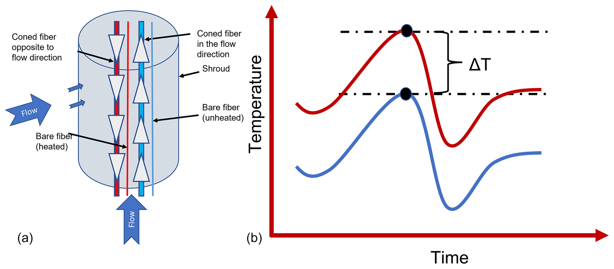
Figure 3(a) Microstructure approach to detecting vertical wind direction using coned FO cables inside the cylindrical shroud. Assuming updraft, the left fiber (indicated in red) would be warmer than the right fiber (shown in blue) due to the cones' direction. (b) Microscopic approach – ΔT determined by wind direction.
2.6 Coherent structure detection using the quadrant analysis method
Coherent structures in tree canopies are defined as spatially coherent motions generated with vertical wind shear, typically associated with strong vertical motions. Every coherent structure event can be divided into upward and downward motions called ejection and sweep phases (Thomas et al., 2017). This study uses coherent structure events to compare the FODS vertical wind signals against observation. The quadrant analysis method, in combination with hyperbolic thresholding, was used to determine the coherent structures. This method uses a scatterplot of two variables (as horizontal (u′) and vertical (w′) wind speed perturbation) in a two-dimensional plane in which the coordinate of each flow variable determines the quadrant defined as Q1(u′>0, w′>0), Q2(u′<0, w′>0), Q3(u′<0, w′<0), and Q4(u′>0, w′<0). The positive direction of w is upward, and if the azimuth angle of the measurement device is zero, the positive direction of u is eastward. The hyperbolic threshold also defines as , where σu and σw are horizontal and vertical wind speed standard deviations, which applied to select the events exceeding the specific hole size (Thomas and Foken, 2007). The 20 Hz data of the sonic anemometer placed at 4 m above ground level at the main tower (as described in Sect. 2.1.2) were used to detect the coherent structure. The outliers were removed from sonic anemometer data, dropping the range of the data outer of ±6σ, assuming a normal distribution. Based on the flow statistic in the Waldstein forest, the perturbation timescale of 10 min was used to compute turbulence quantities. The three-dimensional coordinate rotation was applied to compute the fluxes and quadrant analysis (Wilczak et al., 2001). Since the horizontal and vertical wind are decorrelated, the coherent structure events located in Q2 having a |L|>0.5 were defined as the ejection phase, and the events located in Q4 having |L|>0.5 were defined as the sweep phase (Thomas and Foken, 2007).
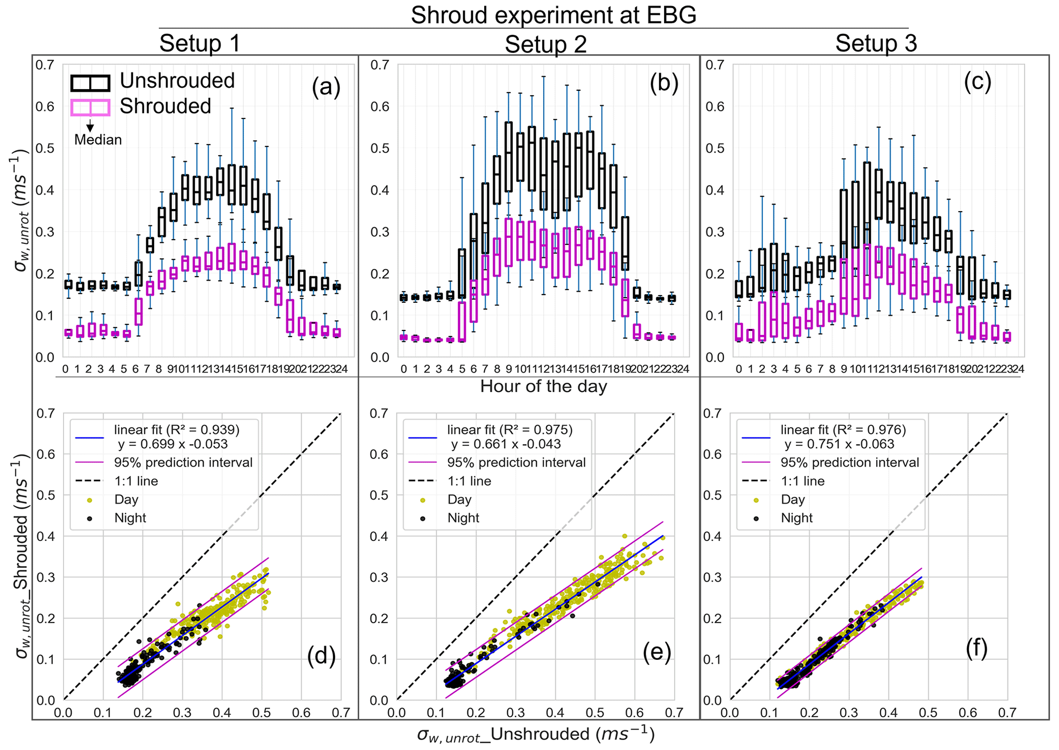
Figure 4(a, d) Diurnal cycle of unrotated vertical wind speed standard deviation (σw, unrot) and scatterplots between σw, unrot shrouded and σw, unrot unshrouded for setup 1 of the shroud experiment at EBG. Panels (b), (e) and (c), (f) show setup 2 and 3, respectively. A 10 min statistic was used to compare the setups. Black and yellow solid points separate night- and daytime. The linear prediction and 95 prediction intervals are shown with solid blue and magenta lines.
2.7 Distributed sensible heat flux using FODS
The sensible heat flux from FODS is the product of instantaneous (e.g., 6 s) vertical wind perturbation () and 6 s temperature perturbation (), which are defined as and , <w> being the 6 s vertical wind speed calculated using the regression of temperature differences between the upward- and downward-pointing coned fibers and vertical wind speed of the sonic anemometer. is the mean of the vertical wind speed over both perturbation timescale (10 min) and length along the fiber (LAF). Similarly, is the mean of air temperature observed with bare unheated fibers over both perturbation timescale (10 min) and LAF. We show the averaged instantaneous variables inside <>, spatially averaged variables with <>, and averaged over time with an overbar. Sensible heat flux from FODS is without averaging overbar, since the perturbations from FODS are spatiotemporally averaged perturbations mostly affected by coherent structures, while in the case of eddy covariance fluxes, we use , since the sonic anemometer perturbations have an inherent physical averaging by its response time. and are vertical wind and sonic temperature perturbations with the original sampling frequency of 20 Hz for the main tower and 10 Hz for the turbulence tower.
3.1 Shroud experiment over grassland
During the shroud experiment at EBG, three experimental setups were tested to compare flow statistics between shrouded and unshrouded sensors (Table 1). At first glance, all of the shroud configurations appear to significantly reduce the vertical wind standard deviation while keeping a good correspondence between σw inside and outside the shroud, decreasing during the night and increasing during daytimes (Fig. 4a, b, and c). The scatterplot between the shrouded and unshrouded σw shown in Fig. 4d, e, and f confirms a high linear relationship (e.g., R2>0.9). The coefficient of determination (R2) in setups 2 and 3 with 0.975 and 0.976 reveals that the shroud with a 60 cm diameter reduces the vertical wind standard deviation less than the 1 m diameter shroud. Also, setup 3 is less scattered where the 95 % prediction interval is narrower compared to other setups. A prediction interval is a type of confidence that predicts the value of a new observation based on your existing model (Neter et al., 1996). The root mean square error (RMSE) shown in Table 1 shows the lowest error of 0.01 ms−1 for daytime and 0.02 ms−1 for nighttime for setup 3. Note that the unrotated wind statistics are used for comparisons, since the reduced horizontal wind speed inside the shroud caused unphysical results when applying coordinate rotation.
Table 1Coefficient of determination and RMSE between total wind speed, horizontal wind speed standard deviation, and vertical wind standard deviations with and without shroud setup, with N being the number of averaging intervals of 10 min statistic. RP is the reduction percentage of each component within the shroud in comparison to the outside of the shroud. RMSE is calculated between data and the linear fit. The RMSE for each variable is shown in a range referring to the RMSE of daytime and nighttime data. The observational period is 15 April to 15 June 2020.
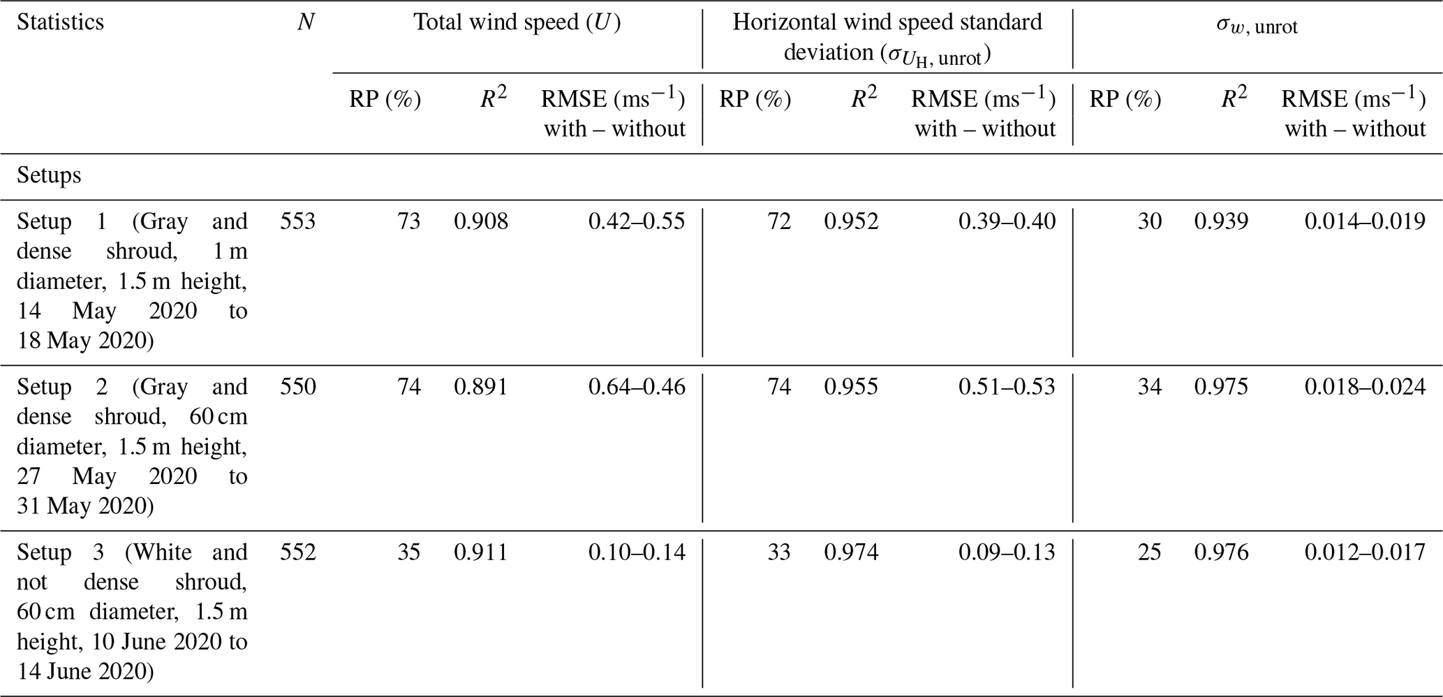
Besides vertical wind speed, the total () and horizontal wind speeds () are included in the comparison of setups (Table 1), where u and v are horizontal wind speed and w is vertical wind speed. Setups 1 and 2 reduce U and UH by 72 % and 74 %, which induces a 30 % and 34 % reduction in the vertical wind standard deviation, while in setup 3, the reduction is 35 % for total and horizontal wind speed and 25 % for vertical wind standard deviation. In terms of coefficient of determination and RMSE, the third setup has higher R2, while having a lower RMSE than the other setups. However, using a 60 cm diameter dense shroud reduces horizontal and vertical wind speed (w) more than the third setup but reduces the goodness of fit between shrouded and unshrouded wind components significantly.
Spectral analysis was performed to compare the shrouded and unshrouded instruments for the third setup to investigate the frequency-specific impacts. Figure 5a and b show that the cylindrical shroud around a sonic anemometer reduces the energy in the integral scales (low frequencies) in both spectra and cospectra. In the inertial subrange, the energy decay slope for both shrouded and unshrouded setups remains mostly for spectra and for cospectra, which is consistent with Kolmogorov (1941). It confirms that the shroud has a minimal effect on the isotropic homogenous eddies in the inertial subrange. The significant effect of the shroud can be seen in the high frequencies closer toward the dissipation scales, where the shrouded and unshrouded spectra and cospectra deviate from each other significantly (Fig. 5c, d). The ratios decrease exponentially for high frequencies, which means the shroud dampens the high-frequency eddies extremely. There is a fixed ratio of spectral energy reduction in the low frequencies for temperature and wind components, momentum, and sensible heat flux in both spectral densities. The Pettitt test detected the timescale of the change point at which the spectral energy decreases abruptly. The change points are shown in Fig. 5c, d, with vertical dotted lines for each spectrum varying by approximately 2 and 6 s. It means the eddies smaller than 6 s are highly influenced by the shroud and should be considered in further analysis.
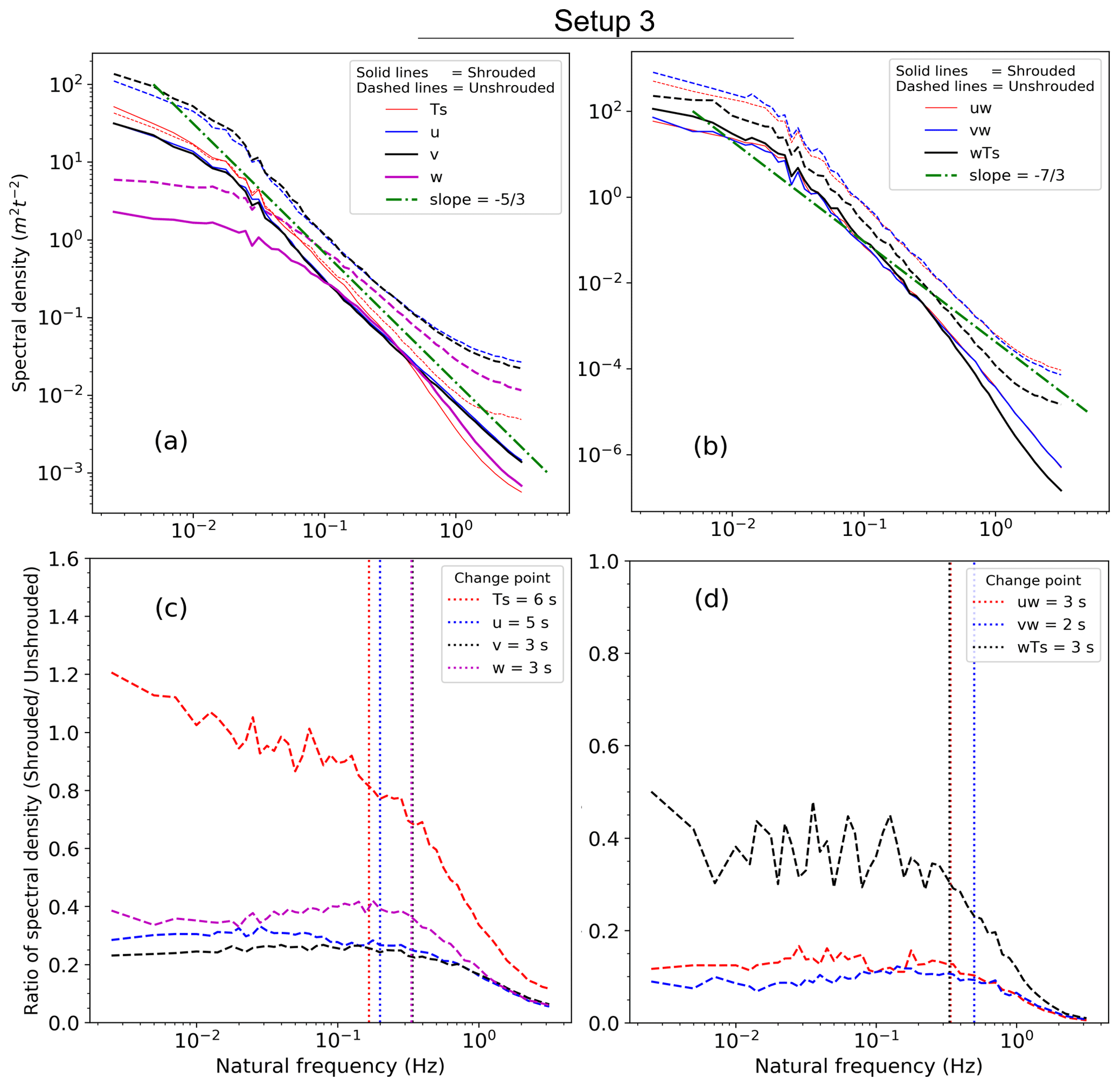
Figure 5(a) The spectra of the wind speed components and the temperature of setup 3 computed every 10 min and ensemble averaged over the period of 5–14 June 2020; (b) the cospectra of the horizontal momentum fluxes, e.g., uw and vw and buoyancy flux, e.g., wTs for the shrouded and unshrouded setups, and uw and vw are the momentum fluxes aligned with u and v, respectively; (c) the ratio of shrouded to unshrouded power spectra; and (d) the ratio of shrouded to unshrouded cospectra specifying the change points with vertical dotted lines. The colors used in (c) and (d) for dashed lines show the same variables in (a) and (b). Ts is the sonic temperature, and v is the horizontal wind speed normal to u.
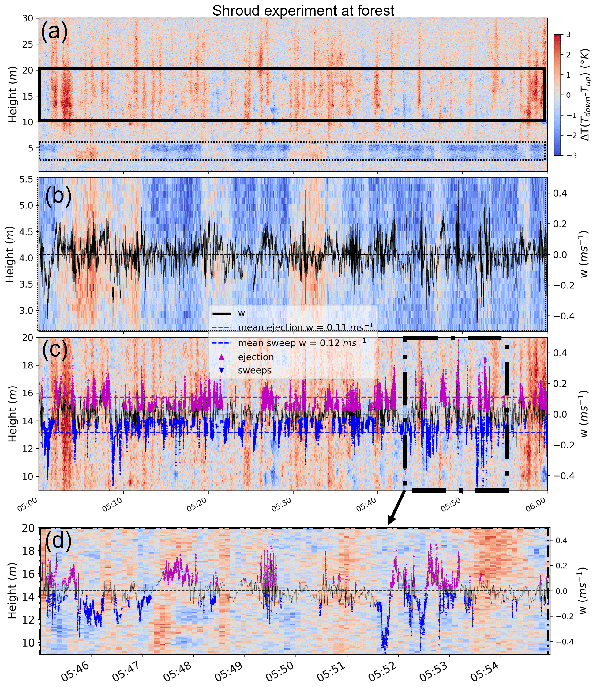
Figure 6(a) Differences in upward-pointing and downward-pointing FODS temperature (ΔT), 6 s time resolution at the main tower during the LOEWE20 experiment on 24 October 2020, 05:00 to 06:00 UTC. The black box with a dashed line shows the location of the shroud installation, and the black box with a solid line shows the comparison section. Panel (b) shows the magnified temperature difference inside the shroud containing 2.75–5.75 m above the ground. The solid black line shows the 20 Hz vertical wind speed of the sonic anemometer installed in the middle of the shroud. Panel (c) shows the magnified temperature within the solid black box in (a), the height range where the minimum horizontal wind speed occurs in the subcanopy. The magenta upward arrows show the vertical wind during the ejection phase, and the blue downward arrows show the vertical wind during the sweep phase extracted using 20 Hz sampled data at a 4 m height. Panel (d) shows the zoomed-in dashed–dotted black box in (c).
3.2 Shroud experiment in the forest
The third shroud setup from the grassland testing site was identified as the most promising and was subsequently deployed during the LOEWE20 experiment in the forest around coned FO cables to evaluate if the vertical wind component could be observed using a combination of the shroud setup and heated coned fibers. We made one modification to the shroud configuration by increasing the length of the shroud from 1.5 m at EBG to 3 m for the forest environment to account for the minimum resolvable scale; the fiber-optic cable and DTS device used in this experiment is 30 s (Freundorfer et al., 2021). In the preparatory phase of the experiment, our analyses yielded a mean magnitude of the vertical wind speed perturbations of 0.1 ms−1 for the Waldstein subcanopy site; hence a shroud length of at least 30 s ⋅ 0.1 ms m seemed optimal to sample the passing eddies by FODS. The turbulence spectrum in rough forest canopies is dominated by organized turbulent motions resulting in more low-frequency turbulence compared to short-vegetated grasslands; hence the integral length scale is larger. This adjustment seemed necessary to capture the main energy-containing eddies. Figure 6a shows a series of reddish and bluish strips of ΔT within both boxes, most likely induced by stronger updrafts and downdrafts, respectively. The depicted structures outside the shroud are clear and more organized than within the shroud and reflect the vertical air movements better than inside the shroud. Figure 6b magnifies the inside of the shroud, adding instantaneous vertical wind speed to give an idea of how ΔT responds to vertical wind speed change once there is no apparent correlation between the two. The correlation coefficient between ΔT and w(ρw) in the main tower is 0.02 inside the shroud but increases to 0.35 outside, demonstrating the substantial increase in correlation between ΔT and w outside the shroud, where the horizontal wind speed in the subcanopy is at its lowest. The ρw coefficient further improved when the data subsampled based on rolling five window correlations between ΔT and w(ρroll) more than 0.8, increasing to 0.53 at the main tower outside the shroud and 0.62 at the turbulence tower.
However, the subsampling significantly improved the correlation outside the shroud for both towers, but no improvements were made inside the shroud, as shown in Fig. 7a. The ΔT within the shroud does not show a good agreement with vertical wind speed, and the results show the failure of the shroud configurations used in the forest experiment to achieve the research objectives. Potential reasons for the failure of this method can be summarized as follows: (i) the 3 m long shroud might act differently than the 1.5 m shroud to suppress the eddies that are passing through the shroud, and (ii) the percentage of the shroud's horizontal wind reduction is not large enough to keep the horizontal wind speed below the speed observed with coned fibers inside the shroud. (iii) Strong vertical motions resulting from passing coherent structures, which are expected to induce an explicit ΔT at greater heights, may slow down when approaching the ground from above the canopy in the sweep phases and do not accelerate enough at the shroud height during the ejection phase. The findings of Thomas and Foken (2007), who studied flux contributions of coherent structures at this site, support this argument, because sensible heat fluxes are well coupled within the canopy up to a height of 0.72 h, h being the canopy, with a relative contribution of nearly 70 %, whereas at lower heights (e.g., 0.29 h), the contribution decreases to approximately 40 % due to weakly coupled top and subcanopy.

Figure 7(a) Scatterplot between 6 s averaged vertical wind speed (<w>) of a sonic anemometer at a 4 m height and ΔT inside the shroud (3–5 m height) for the whole period shown in yellow and subsampled with ρroll>0.8 with black. The error bars show the median with a solid point with two whiskers at ±σ. (b) The same scatterplot as (a) but outside the shroud at 12–17 m above ground level at the main tower. (c) The same scatterplot as (b) but for turbulence tower. The error bars are based on the ensemble average of w over ΔT with a bin size of 0.03 ∘C, and the fit lines are based on the median points for each bin. The data of 24 October 2020, 01:00 to 08:00 UTC, were used to produce the scatterplots. All the data in scatterplots are limited to the 99 % percentile.
Figure 8(a) Scatterplot between horizontal wind speed computed using FODS and ΔT both averaged at the 12–17 m above ground level at the turbulence tower. (b) The same plot as (a) but using the wind speed from a sonic anemometer at 36 m. See Fig. 7's caption for the error bar and data information.

Figure 9Distributed sensible heat flux estimates from FODS averaged over 5 min at the main and turbulence tower on 24 October 2020, 01:00 to 08:00 UTC. Our approach utilizes a linear regression between ΔT drove from coned fibers and w from a sonic anemometer at 36 m to calculate distributed w. The temperature of unheated bare fiber is used as distributed air temperature.
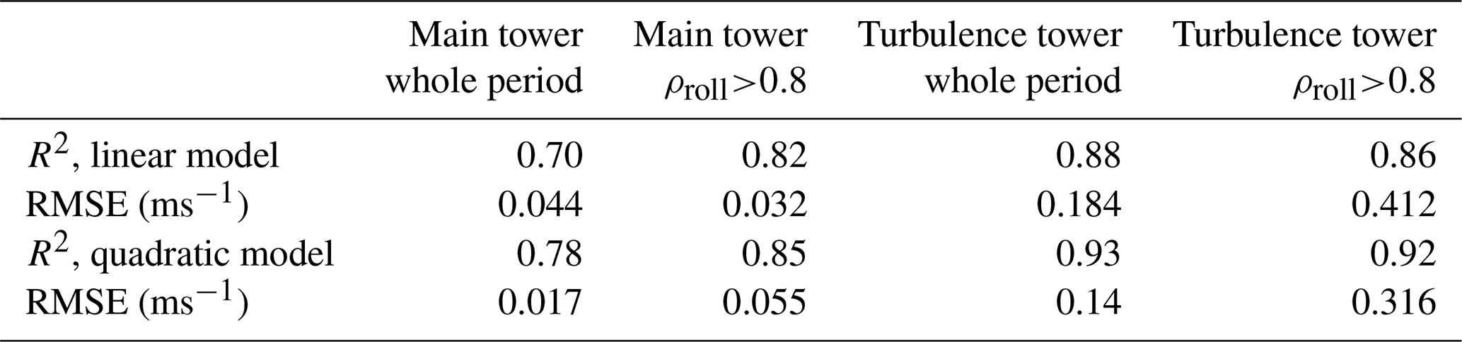
The analysis of the optimum shroud configuration at the forest failed to observe the sign and magnitude of the vertical wind perturbation using FODS; however, conducting this experiment coincided with an unexpected discovery that the heated coned fibers could observe the coherent structure events in the weak-wind subcanopy outside the shroud within the heights where the minimum horizontal wind speed occurs in the subcanopy. See Fig. S1 in the Supplement for the distributed wind speed profile calculated with FODS for the period of the data used in this study. Figure 6c and d show the mentioned height range together with the sweep and ejection phases, illustrating a good agreement between the positive ΔT with ejection phases and negative ΔT with the sweep phases. The magenta and blue arrows follow the reddish and blueish ΔT's, where higher vertical wind speeds are accompanied by solid features of reddish or blueish stripes, which indicates the duration of coherent structures, while the color intensity might represent the vertical wind speed of motions. In contrast, conditional sampling does not improve the correlation between ΔT and w inside the shroud (Fig. 7a). Note that the sonic anemometer data at a 4 m height were used to compute the correlation coefficients with a section of FODS data at the main tower at 12 to 17 m, adding two sources of uncertainty to the correlation. First, there may be a time lag between two measurements because of height differences, and second, the two heights may not be well coupled, so strong vertical movements of air at a 12–17 m height might dissipate or weaken at 4 m. The mentioned limitation at the main tower is expected to be less at the turbulence tower, since the sonic anemometer is placed at 36 m above the canopy level, where there is a robust sensible flux coupling between these two heights based on Thomas and Foken (2007). The scatterplot between ΔT and w shown in Fig. 7b and c confirms a slight positive correlation between ΔT and w with ρw=0.35 and 0.36 at the main and turbulence tower for the whole selected period shown in yellow, respectively. This correlation improves under certain situations: for instance, the correlation coefficient increases to 0.53 and 0.62 when conditional subsampling is used based on the rolling five-window correlation of ΔT and w(ρroll) greater than 0.8 (shown in black in Fig. 7b and c). The best fit for the median of ensembled w over ΔT is the quadratic function for both towers with an R2 of 0.78 and 0.93 and an RMSE of 0.02 and 0.14 ms−1 for the main and turbulence tower. The quadratic relation between w and ΔT is in line with similar equations describing the relation between convective heat loss from the fiber-optic cable and horizontal wind speed, including Sayde et al. (2015) and Van Ramshorst et al. (2020). The linear model is also the second best-fit model to the median points of the ensemble vertical wind speeds over the ΔT with an R2 of 0.70 and 0.88 and an RMSE of 0.04 and 0.18 for main and turbulence towers (Table 3). The height of the error bar in Fig. 7a and b remains almost the same at different ΔT, but the scatterplots are more scattered in the low ΔT. The horizontal wind speed was found as the main reason for the deteriorating ΔT signal, where the lowest horizontal wind speed shows smaller error bars (Fig. 8a and b). However, the horizontal wind speed of less than 0.3 ms−1 at the subcanopy includes a few percent of the data, which were insufficient to separate and analyze the relationships within these periods.

Figure 10(a, b) Time series and (c, d) scatterplot of the sensible heat fluxes observed with the sonic anemometer and from FODS for heights between 12 and 17 m, which is the height where the horizontal wind speed is minimum.
Table 2Coefficient of determination (R2) and RMSE between quadratic and linear fit on the median points at Fig. 7 for the whole period and ρroll>0.8, ρroll being the rolling correlations between ΔT and w. The number of data used to compute the R2 and RMSE was N=62 for all cases. The same data as Fig. 7 were used for computation.
Following the comparison between ΔT and w for a selected 7 h data for both main and turbulence towers, we evaluated the dataset for the percentage of correctly detected vertical wind directions, which is calculated as a fraction of the number of vertical wind directions that were successfully observed using FODS to the number of chosen data (F). A section of 5 m length of FODS ΔT from 12 to 17 m above ground level was selected and compared against sonic anemometer vertical wind direction to compute the F. Table 3 shows F for whole data and when the five-window rolling correlation (ρroll) between ΔT and w is larger than 0.8. The analyzed data shows 60 % and 63 % F at the main and turbulence towers, respectively, which increases to 71 % and 67 % for ρroll>0.8. Since we know the sign of the distributed vertical wind perturbation with a defined F, we can compute the magnitude of the distributed vertical wind speed perturbations from the relationship between vertical wind speed and ΔT with a known correlation coefficient and have distributed air temperature perturbations directly observed from the unheated FO cable across the entire canopy; we computed the distributed sensible heat fluxes () solely based on FODS using the linear and quadratic regression between w and ΔT in Fig. 7b and c to compute the vertical wind perturbation () for the unshrouded section. The distributed heat flux in Fig. 9 is based on a linear regression between <w> and ΔT at the turbulence and main towers, which yields an RMSE of 0.001 and 0.01 Kms−1 in comparison with the sonic anemometer's buoyancy heat flux (). However, the RMSE is lower at the main tower, but the computed flux is independent of observation with a correlation of 0.04, whereas the correlation is 0.26 at the turbulence tower. Despite the many assumptions creating uncertainty in computing distributed sensible heat flux, the range and temporal dynamics of the computed fluxes across techniques match well for this selected period. We observe two areas with distinct differences (Fig. 9): (i) the area near to the ground up to about 7 m where the fluxes are negative and downward; interestingly, the features are more pronounced between 05:00 and 06:00 UTC when the horizontal wind is weaker, and (ii) the height between 9 and 20 m, where the fluxes are often positive and upward, and the features of updrafts are discernible most of the time, since the horizontal wind speed at the mentioned height remains below the threshold (∼0.30 ms−1 Fig. 8a). The comparison also confirms that the computed sensible heat fluxes are in the range of the estimates from classic eddy covariance using sonic anemometry, but, still, the method has some bias in heat flux with an RMSE of 0.01 and 0.0009 Kms−1 for the turbulence and main tower, respectively (Fig. 10). As discussed in Sect. 2.7, the fluxes shown as and in this study are not expected to be identical, as they represent different parts of the forest canopy volume. This first presentation of spatially distributed sensible heat fluxes using FODS solely reinforces the utility of the microstructure approach to directly observe vertical wind component with higher accuracy.
This study examined the potential of a physical shroud constructed around heated and unheated fiber-optic cables to overcome the limitations of the microstructure approach caused by the much stronger horizontal wind speed to observe the distributed vertical wind component from FODS. We arrive at the following conclusions:
- i
Comparison between different shrouds in shape, color, rigidity, and porosity suggested that the white shroud with a 0.60 m diameter is the optimum shroud suitable for filtering the horizontal wind speed by 35 % while having minimal effect on vertical wind speed.
- ii
The spectral analysis between shrouded and unshrouded setups showed a significant energy reduction dissipation range. This reduction is minor in the inertial subrange, and both shrouded and unshrouded spectra obey the energy decay law. The spectra ratio between shrouded and unshrouded setups revealed that the eddies smaller than 6 s are extremely damped within the shroud.
- iii
Validating the promising shroud setup by adding heated coned fibers inside showed that the shroud fails to keep the vertical wind signal. This failure could be because (i) the shroud does not reduce the horizontal wind speed below the threshold so that the coned fibers can sense the signal. (ii) The shroud's increased length to 3 m changes the behavior of the shroud against the eddies in comparison with a 1.5 m shroud and causes suppression of the eddies that are dominant at the shroud height. (iii) The shroud installation height is not dominant with the same strong, coherent structures as the comparison section (12–17 m).
- iv
In contrast, evaluation of FODS observations from unshrouded paired coned and heated and unheated FO cables revealed that there is a height range in the subcanopy (12–17 m) where the ΔT from coned fibers show good agreement to sonic anemometer observations. This agreement is more significant during the vertical air movement of coherent structures (e.g., sweep and ejection phases). Within the mentioned height range, the heated coned fiber is capable of detecting the vertical wind direction at least 60 % of the time. The vertical wind speed also has a correlation of 0.35 with the temperature difference between up- and down-pointing fibers, which improves up to 0.62 with conditional sampling.
- v
The distributed sensible heat flux was computed using the linear and quadratic regression of ΔT and w. Nonetheless, the distributed sensible heat flux seems within the plausible range of the measured fluxes with eddy covariance but still needs improvement. The spatial structure of the distributed sensible heat flux shows explicit information about flux distribution along with the canopy height and changing the sign of the flux at about a 7 m height. This study could be followed with further improvements by adjusting the cone shape and size to increase the correlation of ΔT and vertical wind direction and wind speed. Additionally, deploying DTS instruments with a high signal-to-noise ratio (SNR) and an FO cable with a low response time would lower the uncertainty.
- vi
This observational achievement is an important step toward developing a FODS-based flux sensor capable of resolving heat flux continuously across spatial and temporal scales.
The dataset is available on Zenodo: https://doi.org/10.5281/zenodo.6913436 (Abdoli et al., 2022).
The supplement related to this article is available online at: https://doi.org/10.5194/amt-16-809-2023-supplement.
Conceptualization: MA, KL, CKT; methodology and manufacturing: MA, CKT, KL, JS, and JO; field data collection: MA, KL, and JS; validation: MA; formal analysis: MA; investigation: MA and CKT; data curation: MA; writing – original draft preparation: MA; writing – review and editing: all authors; visualization: MA; project administration: CKT and MA; funding acquisition: CKT. All authors have read and agreed to the published version of the paper.
The contact author has declared that none of the authors has any competing interests.
Publisher's note: Copernicus Publications remains neutral with regard to jurisdictional claims in published maps and institutional affiliations.
This research has been supported by the European Research Council, H2020 European Research Council (DarkMix (grant no. 724629)).
This open-access publication was funded by the University of Bayreuth.
This paper was edited by Cléo Quaresma Dias-Junior and reviewed by three anonymous referees.
Abdoli, M., Lapo, K., Schneider, J., Johannes, and Thomas, C.: Shroud Experiment 2020 (Version 1.0), Zenodo [data set], https://doi.org/10.5281/ZENODO.6913436, 2022.
Anfossi, D., Oettl, D., Degrazia, G., and Goulart, A.: An analysis of sonic anemometer observations in low wind speed conditions, Bound.-Lay. Meteorol., 114, 179–203, https://doi.org/10.1007/s10546-004-1984-4, 2005.
Brunet, Y.: Turbulent Flow in Plant Canopies: Historical Perspective and Overview, Bound.-Lay. Meteorol., 177, 315–364, https://doi.org/10.1007/S10546-020-00560-7, 2020.
Burgers, J. M.: A Mathematical Model Illustrating the Theory of Turbulence, Adv. Appl. Mech., 1, 171–199, https://doi.org/10.1016/S0065-2156(08)70100-5, 1948.
Cheng, Y., Sayde, C., Li, Q., Basara, J., Selker, J., Tanner, E., and Gentine, P.: Failure of Taylor's hypothesis in the atmospheric surface layer and its correction for eddy-covariance measurements, Geophys. Res. Lett., 44, 4287–4295, https://doi.org/10.1002/2017GL073499, 2017.
Corrsin, S.: Turbulent Flow, Am. Sci., 49, 300–325, 1961.
Engelmann, C. and Bernhofer, C.: Exploring Eddy-Covariance Measurements Using a Spatial Approach: The Eddy Matrix, Boundary-Layer Meteorol., 161, 1–17, https://doi.org/10.1007/s10546-016-0161-x, 2016.
Foken, T., Serafimovich, A., Eder, F., Hübner, J., Gao, Z., and Liu, H.: Energy and Matter Fluxes of a Spruce Forest Ecosystem, 229, 309–329, 2017.
Foken, T., Babel, W., Munger, J. W., Grönholm, T., Vesala, T., and Knohl, A.: Selected breakpoints of net forest carbon uptake at four eddy-covariance sites, Stock. Uni Press, 73, 1–12, https://doi.org/10.1080/16000889.2021.1915648, 2021.
Freundorfer, A., Lapo, K., Schneider, J., and Thomas, C. K.: Distributed sensing of wind direction using fiber-optic cables, J. Atmos. Ocean. Technol., 38, 1871–1883, https://doi.org/10.1175/jtech-d-21-0019.1, 2021.
Fritz, A. M., Lapo, K., Freundorfer, A., Linhardt, T., and Thomas, C. K.: Revealing the Morning Transition in the Mountain Boundary Layer Using Fiber-Optic Distributed Temperature Sensing, Geophys. Res. Lett., 48, 1–11, https://doi.org/10.1029/2020GL092238, 2021.
Grachev, A. A., Andreas, E. L., Fairall, C. W., Guest, P. S., and Persson, P. O. G.: The Critical Richardson Number and Limits of Applicability of Local Similarity Theory in the Stable Boundary Layer, Bound.-Lay. Meteorol., 147, 51–82, https://doi.org/10.1007/s10546-012-9771-0, 2013.
Kolmogorov, A. N.: Energy dissipation in locally isotropic turbulence, Dokl. Akad. Nauk. SSSR, 32, 19–21, 1941.
Lapo, K. and Freundorfer, A.: klapo/pyfocs v0.5, Zenodo [code], https://doi.org/10.5281/ZENODO.4292491, 26 November 2020.
Lapo, K., Freundorfer, A., Pfister, L., Schneider, J., Selker, J., and Thomas, C.: Distributed observations of wind direction using microstructures attached to actively heated fiber-optic cables, Atmos. Meas. Tech., 13, 1563–1573, https://doi.org/10.5194/amt-13-1563-2020, 2020.
Liang, J., Zhang, L., Wang, Y., Cao, X., Zhang, Q., Wang, H., and Zhang, B.: Turbulence regimes and the validity of similarity theory in the stable boundary layer over complex terrain of the Loess Plateau, China, Wiley Online Libr., 119, 6009–6021, https://doi.org/10.1002/2014JD021510, 2014.
Mahrt, L., Thomas, C., Richardson, S., Seaman, N., Stauffer, D., and Zeeman, M.: Non-stationary Generation of Weak Turbulence for Very Stable and Weak-Wind Conditions, Bound.-Lay. Meteorol., 147, 179–199, https://doi.org/10.1007/s10546-012-9782-x, 2013.
Neter, J., Kutner, M., Nachtsheim, C., and Wasserman, W.: Applied linear statistical models, ISBN 13 9780256117363, 1996.
Pettitt, A. N.: A Non-Parametric Approach to the Change-Point Problem, J. R. Stat. Soc. Ser. C, 28, 126–135, https://doi.org/10.2307/2346729, 1979.
Pfister, L., Lapo, K., Mahrt, L., and Thomas, C. K.: Thermal Submeso Motions in the Nocturnal Stable Boundary Layer. Part 2: Generating Mechanisms and Implications, Boundary-Layer Meteorol., 180, 203–224, https://doi.org/10.1007/s10546-021-00619-z, 2021.
Predosa, R.: Lasers in the Sky: Distributed Temperature Sensing and a Micro-Meteorological Approach to Quantifying Evapotranspiration, https://ir.library.oregonstate.edu/concern/graduate_thesis_or_dissertations/hx11xm175?locale=en (last access: 28 January 2017), 17 June 2016.
Sayde, C., Thomas, C. K., Wagner, J., and Selker, J.: High-resolution wind speed measurements using actively heated fiber optics, Geophys. Res. Lett., 42, 10064–10073, https://doi.org/10.1002/2015GL066729, 2015.
Schilperoort, B., Coenders-Gerrits, M., Jiménez Rodríguez, C., van der Tol, C., van de Wiel, B., and Savenije, H.: Decoupling of a Douglas fir canopy: a look into the subcanopy with continuous vertical temperature profiles, Biogeosciences, 17, 6423–6439, https://doi.org/10.5194/bg-17-6423-2020, 2020.
Sun, J., Mahrt, L., Banta, R. M., and Pichugina, Y. L.: Turbulence regimes and turbulence intermittency in the stable boundary layer: During CASES-99, J. Atmos. Sci., 69, 338–351, https://doi.org/10.1175/JAS-D-11-082.1, 2012.
Tennekes, H., Lumley, J., and Lumley, J.: A first course in turbulence, The MIT Press, https://doi.org/10.7551/mitpress/3014.001.0001, 1972.
Thomas, C. and Foken, T.: Flux contribution of coherent structures and its implications for the exchange of energy and matter in a tall spruce canopy, Bound.-Lay. Meteorol., 123, 317–337, https://doi.org/10.1007/s10546-006-9144-7, 2007.
Thomas, C. K.: Variability of Sub-Canopy Flow, Temperature, and Horizontal Advection in Moderately Complex Terrain, Bound.-Lay. Meteorol., 139, 61–81, https://doi.org/10.1007/s10546-010-9578-9, 2011.
Thomas, C. K. and Selker, J.: Optical Fiber-Based Distributed Sensing Methods, Springer Handbooks, 611–633, https://doi.org/10.1007/978-3-030-52171-4_20, 2021.
Thomas, C. K., Law, B. E., Irvine, J., Martin, J. G., Pettijohn, J. C., Davis, K. J., Thomas, C.:, Law, B. E., Irvine, J., Martin, J. G., Pettijohn, J. C., and Davis, K. J.: Seasonal hydrology explains interannual and seasonal variation in carbon and water exchange in a semiarid mature ponderosa pine forest in central Oregon, J. Geophys. Res.-Biogeo., 114, 4006, https://doi.org/10.1029/2009JG001010, 2009.
Thomas, C. K., Kennedy, A. M., Selker, J. S., Moretti, A., Schroth, M. H., Smoot, A. R., Tufillaro, N. B., and Zeeman, M. J.: High-Resolution Fibre-Optic Temperature Sensing: A New Tool to Study the Two-Dimensional Structure of Atmospheric Surface-Layer Flow, Bound.-Lay. Meteorol., 142, 177–192, https://doi.org/10.1007/s10546-011-9672-7, 2012.
Thomas, C. K., Serafimovich, A., Siebicke, L., Gerken, T., and Foken, T.: Coherent Structures and Flux Coupling BT – Energy and Matter Fluxes of a Spruce Forest Ecosystem, edited by: Foken, T., Springer International Publishing, Cham, 113–135, https://doi.org/10.1007/978-3-319-49389-3_6, 2017.
Thomas, C. K., Huss, J. M., Abdoli, M., Huttarsch, T., and Schneider, J.: Solid-Phase Reference Baths for Fiber-Optic Distributed Sensing, Sensors, 22, https://doi.org/10.3390/s22114244, 2022.
van de Giesen, N., Steele-Dunne, S. C., Jansen, J., Hoes, O., Hausner, M. B., Tyler, S., and Selker, J.: Double-Ended Calibration of Fiber-Optic Raman Spectra Distributed Temperature Sensing Data, Sensors, 12, 5471–5485, https://doi.org/10.3390/S120505471, 2012.
Van de Wiel, B. J. H., Moene, A. F., Jonker, H. J. J., Baas, P., Basu, S., Donda, J. M. M., Sun, J., and Holtslag, A. A. M.: The minimum wind speed for sustainable turbulence in the nocturnal boundary layer, J. Atmos. Sci., 69, 3116–3127, https://doi.org/10.1175/JAS-D-12-0107.1, 2012.
van Ramshorst, J. G. V., Coenders-Gerrits, M., Schilperoort, B., van de Wiel, B. J. H., Izett, J. G., Selker, J. S., Higgins, C. W., Savenije, H. H. G., and van de Giesen, N. C.: Revisiting wind speed measurements using actively heated fiber optics: a wind tunnel study, Atmos. Meas. Tech., 13, 5423–5439, https://doi.org/10.5194/amt-13-5423-2020, 2020.
Vickers, D. and Thomas, C. K.: Observations of the scale-dependent turbulence and evaluation of the flux–gradient relationship for sensible heat for a closed Douglas-fir canopy in very weak wind conditions, Atmos. Chem. Phys., 14, 9665–9676, https://doi.org/10.5194/acp-14-9665-2014, 2014.
Wilczak, J. M., Oncley, S. P., and Stage, S. A.: Sonic Anemometer Tilt Correction Algorithms, Bound.-Lay. Meteorol., 99, 127–150, https://doi.org/10.1023/A:1018966204465, 2001.
Zarenistanak, M., Dhorde, A. G., and Kripalani, R. H.: Trend analysis and change point detection of annual and seasonal precipitation and temperature series over southwest Iran, J. Earth Syst. Sci., 123, 281–295, https://doi.org/10.1007/s12040-013-0395-7, 2014.