An optimised organic carbon ∕ elemental carbon (OC ∕ EC) fraction separation method for radiocarbon source apportionment applied to low-loaded Arctic aerosol filters

Radiocarbon (¹⁴C) analysis of carbonaceous aerosols is used for source apportionment, separating the carbon content into fossil vs. non-fossil origin, and is particularly useful when applied to subfractions of total carbon (TC), i.e. elemental carbon (EC), organic carbon (OC), water-soluble OC (WSOC), and water-insoluble OC (WINSOC). However, this requires an unbiased physical separation of these fractions, which is difficult to achieve. Separation of EC from OC using thermal–optical analysis (TOA) can cause EC loss during the OC removal step and form artificial EC from pyrolysis of OC (i.e. so-called charring), both distorting the ¹⁴C analysis of EC. Previous work has shown that water extraction reduces charring. Here, we apply a new combination of a WSOC extraction and ¹⁴C analysis method with an optimised $\mathrm{OC}/\mathrm{EC}$ separation that is coupled with a novel approach of thermal-desorption modelling for compensation of EC losses. As water-soluble components promote the formation of pyrolytic carbon, water extraction was used to minimise the charring artefact of EC and the eluate subjected to chemical wet oxidation to CO₂ before direct ¹⁴C analysis in a gas-accepting accelerator mass spectrometer (AMS). This approach was applied to 13 aerosol filter samples collected at the Arctic Zeppelin Observatory (Svalbard) in 2017 and 2018, covering all seasons, which bear challenges for a simplified ¹⁴C source apportionment due to their low loading and the large portion of pyrolysable species. Our approach provided a mean EC yield of 0.87±0.07 and reduced the charring to 6.5 % of the recovered EC amounts. The mean fraction modern (F¹⁴C) over all seasons was 0.85±0.17 for TC; 0.61±0.17 and 0.66±0.16 for EC before and after correction with the thermal-desorption model, respectively; and 0.81±0.20 for WSOC.

1 Introduction

Considerable efforts have been made to investigate atmospheric aerosol due to its relevance to a wide range of environmental topics, including change in radiative forcing and adverse effects on human health (McNeill, 2017; Lelieveld et al., 2015; Landrigan, 2017; Pope et al., 2020). Exposure to ambient atmospheric particulate matter (PM) has been associated with damage to the cardiopulmonary system and causing at least 3 million premature deaths per year globally (Kim et al., 2015; Lelieveld et al., 2015; GBD 2015 Risk Factors Collaborators, 2016). Understanding aerosols is therefore crucial for future projections and for the improvement of air quality, especially for severely affected areas (Quinn et al., 2008; Bond et al., 2013; Schmale et al., 2021). Although the Arctic is considered a pristine part of the world, it is also affected by emissions from polluted regions in the Northern Hemisphere, causing the Arctic haze phenomenon (Barrie, 1986; Heidam et al., 2004; Quinn et al., 2002; Zhao and Garrett, 2015; Engelmann et al., 2021; Jouan et al., 2014), occurring in late winter and early spring, and which have been known for decades (Barrie et al., 1981). Arctic haze consists mainly of sulfate and carbonaceous aerosols trapped in the cold retracting polar dome in spring, coupled with reduced wet scavenging in winter and spring (Abbatt et al., 2019; Moschos et al., 2022).

Carbonaceous aerosols (here, total carbon, TC) consists of an organic fraction referred to as organic carbon (OC), and a refractory light-absorbing component named elemental carbon (EC) or equivalent black carbon (eBC) when quantified with thermal–optical analysis or optical methods, respectively (Contini et al., 2018; Bond et al., 2013; Petzold et al., 2013). TC constitutes 20 % to 90 % of the aerosol mass (Kanakidou et al., 2005; Putaud et al., 2010; Gentner et al., 2017). As a main PM component, it thus contributes to adverse effects on public health and climate. On the one hand, carbonaceous aerosols may contain toxic or carcinogenic compounds such as polycyclic aromatic hydrocarbons (PAHs) (Mauderly and Chow, 2008; Kim et al., 2013; Smichowski et al., 2005; Daellenbach et al., 2020). On the other hand, both EC and OC are climate relevant: the effective radiative forcing (ERF) for atmospheric aerosols is negative, and while the OC fraction has a negative ERF, the EC fraction has a positive ERF (IPCC, 2021). Overall, the surface albedo for black carbon (BC) and OC on snow and ice is positive with a global mean ERF of 0.08 (0.00 to 0.18) (IPCC, 2021). Consequently, sources of OC, EC, and subfractions must be understood to improve air quality and mitigate adverse effects of carbonaceous aerosols. Due to their complex composition and multitude of sources, however, carbonaceous aerosols are still inadequately understood.

Source apportionment is a widely used approach to gain understanding on the emission, formation, and transformation of carbonaceous aerosols. It investigates the chemical and physical composition of aerosols at receptor sites to disentangle the contributions of individual emissions and the attribution to different source categories. Radiocarbon (¹⁴C) measurements constitute an important source apportionment tool that can unambiguously separate between fossil and contemporary carbon present in carbonaceous aerosol, including in the OC and EC subfractions (Szidat et al., 2006; Winiger et al., 2015; Zotter et al., 2014). Sources of OC and EC are often very different, and such additional information is obtained by means of ¹⁴C source apportionment of both EC and OC compared to a radiocarbon of TC analysis alone. The analysis of the OC subfractions water-soluble OC (WSOC) and water-insoluble OC (WINSOC) can lead to further information on the fossil and non-fossil fractions of the emitting sources (Zhang et al., 2014b).

Separation of OC and EC is method dependent, but the classification is widely recognised (Pöschl, 2003). EC is a primary particle, i.e. emitted directly to the atmosphere and generated by incomplete combustion of fossil fuels and biomass, whereas OC is either primary or secondary, i.e. emitted directly or formed in the atmosphere by oxidation of both anthropogenic and biogenic precursor gases (Kanakidou et al., 2005). Thermal–optical analysis (TOA) is a well-established and commonly used technique for $\mathrm{OC}/\mathrm{EC}$ determination (Chow et al., 2004; Cavalli et al., 2010; Chow et al., 1993; Schmid et al., 2001; Huntzicker et al., 1982; Zenker et al., 2017; Dasari and Widory, 2022). Typically, two or more heating steps in an inert (i.e. helium) and in an oxidative atmosphere (i.e. 2 % oxygen in helium) are used to desorb OC and EC, respectively. During analysis, the transmission or reflectance of the filter sample is continuously measured (Birch and Cary, 1996; Schmid et al., 2001). A change in the transmission or reflectance signal indicates charring and EC loss. Charring is known as the process when OC pyrolyses and forms pyrolytic carbon (PC) that shows similar optical properties to EC, thus decreasing the transmission signal and creating a positive EC artefact (Cadle et al., 1980; Yu et al., 2002; Chow et al., 2004; Boparai et al., 2008). Charring leads to an overestimation of EC and an underestimation of OC. Additionally to charring, some EC is lost by desorption during thermal separation of OC, leading to a negative EC artefact. Both the positive EC artefact (i.e. charring) and the negative artefact (i.e. partial EC loss) may induce a bias in ¹⁴C measurement of EC. Charring adds OC, which is typically has a higher non-fossil proportion than EC (Szidat et al., 2006, 2009; Zhang et al., 2012, 2014b; Zotter et al., 2014; Vlachou et al., 2018), so that the measured ¹⁴C of EC may appear to have a higher non-fossil proportion than it does. Partial EC loss usually affects non-fossil EC (e.g. from biomass burning) more than fossil EC (e.g. from traffic or coal combustion) so that the remaining EC may be altered and seem to have a higher fossil proportion. Correction of both artefacts is therefore required for the accurate quantification of the fossil vs. non-fossil shares of EC. EC recovery after $\mathrm{OC}/\mathrm{EC}$ separation is determined using the transmission or reflectance signal (Gundel et al., 1984; Zhang et al., 2012). Frequently used TOA protocols for $\mathrm{OC}/\mathrm{EC}$ determination include EUSAAR_2 (Cavalli et al., 2010), IMPROVE (Chow et al., 1993), and NIOSH (Eller and Cassinelli, 1996). Radiocarbon measurement requires a clear physical separation of OC and EC, since OC and EC do not originate from the same processes and often show very different radiocarbon signatures (Szidat et al., 2006, 2007; Zhang et al., 2014b). Traditional TOA protocols may still contain some OC in charred or an unaltered form after the split point and thus fail to perform the physical separation adequately for radiocarbon source apportionment (Barrett et al., 2015; Zhang et al., 2012). Gustafsson et al. (2001) developed a separation technique (CTO-375) in soil sediments, which was later applied to radiocarbon source apportionment of atmospheric aerosols (Zencak et al., 2007). A two-step separation method developed by Szidat et al. (2004b) was utilised for radiocarbon source apportionment (Zhang et al., 2010; Jenk et al., 2007; Szidat et al., 2004b). As these simplified approaches still failed to provide isolation of EC, our group (Zhang et al., 2012) established an improved four-step method (Swiss_4S) that aimed at a best-possible congruence with existing TOA protocols (especially with EUSAAR_2) and additionally used water extraction before TOA and pure O₂ for an optimised EC recovery and reduced charring. Nevertheless, the quantification of EC losses and PC formation remains a challenge, as both fractions and processes typically overlap each other and can hardly be distinguished from each other (Boparai et al., 2008). Later, Agrios et al. (2015) coupled the Sunset thermo-optical $\mathrm{OC}/\mathrm{EC}$ analyser with online measurement in an accelerator mass spectrometer (AMS) and implemented the previously developed Swiss_4S protocol.

Many have investigated EC in the Arctic including stable isotope (¹³C) and radiocarbon analysis for source apportionment (Winiger et al., 2016, 2017, 2015; Moschos et al., 2021). The fossil contribution of OC and WSOC is often not measured directly but calculated by the isotope mass balance approach (Vlachou et al., 2018). Zhang et al. (2014a) lyophilised and re-solubilised the eluate from water extraction before combustion in an elemental analyser coupled with radiocarbon measurement. Menzel and Vaccaro (1964) as well as Sharp (1973) used potassium persulfate for the oxidation of dissolved organic carbon in seawater. Lang et al. (2012) employed such a chemical wet oxidation for stable isotope analysis of dissolved organic matter in freshwater samples. This method was later used for stable and radiocarbon analysis of marine samples as well as compound-specific analysis of pyrogenic carbon (Lang et al., 2013; Wiedemeier et al., 2016), but it has not been adapted for ¹⁴C analysis of WSOC from carbonaceous aerosols so far.

The present study provides a framework for an optimal $\mathrm{OC}/\mathrm{EC}$ separation and radiocarbon analysis coupled with direct ¹⁴C(WSOC) analysis (i.e. the ¹⁴C analysis of WSOC) by chemical wet oxidation applied on low-loaded Arctic filters. We provide a novel method for the EC yield extrapolation and charring correction based on a chemical desorption model that represents the behaviour of EC from different sources more realistically. Arctic filters were utilised as they are challenging for radiocarbon analysis due to their low loading and the large portion of pyrolysable species. Using an optimised strategy, we can measure the F¹⁴C value (i.e. the fraction modern) in all major aerosol filter fractions (TC, EC, WSOC, WINSOC) with the lowest possible amount of filter material if sufficient filter loading is provided.

2 Experimental

2.1 Overview of the analytical procedures

Aerosol filter samples were first water-extracted to collect WSOC for subsequent radiocarbon measurement and to minimise formation of PC, caused primarily by WSOC, otherwise causing a dilution of the true ¹⁴C(EC) signal. We then used the first three steps of the Swiss_4S protocol (Zhang et al., 2012) to remove WINSOC from the filter by thermal–optical analysis, isolating EC. The filter's EC content was evolved by total combustion in a TOA analyser and subjected to online radiocarbon measurements. The WSOC eluate was converted to CO₂ by chemical wet oxidation before radiocarbon measurement. The following sections explain the different procedures in brief, whereas the Supplement provides information that is more detailed.

2.2 Sampling and filter selection

Aerosol filter samples were collected between February 2017 and November 2018 at the Zeppelin Observatory (Svalbard) (78^∘54^′ N, 11^∘52^′ E; 475 m a.s.l.), which is part of the Global Atmospheric Watch (GAW) programme, the Arctic Monitoring and Assessment Programme (AMAP), and the European Evaluation and Monitoring Programme (EMEP) (Hung et al., 2010; Tørseth et al., 2012; Platt et al., 2022). Aerosol particles were collected on pre-fired (850 ^∘C, 3 h) quartz fibre filters (Pallflex^® Tissuquartz 2500QAT-UP; 150 mm in diameter) downstream of a PM₁₀ inlet, using a Digitel high-volume sampler (DH-77, Hegenau, Switzerland). The sampler operated at a flow rate of 689 L min⁻¹, corresponding to an air volume of 6945 m³ for a sampling time of 1 week. Filter samples were collected according to the quartz-behind-quartz (QBQ) setup (McDow and Huntzicker, 1990), allowing for an estimate of the positive sampling artefact of OC.

A fraction (46 mm diameter, corresponding to 16.6 cm²) of the total filter area (153.9 cm²) were cut for radiocarbon measurement of ¹⁴C(TC), ¹⁴C(WSOC), and ¹⁴C(EC) (Fig. 1). The filter's TC, EC, and OC contents were quantified according to the EUSAAR_2 temperature programme (Cavalli et al., 2010), using transmission for charring correction. A total of 18 filter samples were received for radiocarbon measurement, but due to low EC loadings, pooling of 5 subsequent filters was necessary (Fig. 1). Owing to the low filter loading, the water extraction for ¹⁴C(WSOC) and ¹⁴C(EC) was only performed on the front filters, whereas ¹⁴C(TC) analysis was performed on both front and back filters.

Figure 1 Separation of the different fractions for ¹⁴C analysis starting from the aerosol filters. One or multiple circular quartz fibre filter punches are stacked and intercalated in the water extraction setup. The residual filter material is used for WINSOC and EC analysis after drying, and the extract is oxidised by chemical wet oxidation. The remaining filter material is used for TC analysis.

2.3 Water extraction

Three circular punches of 22 mm (diameter) made from the 46 mm (diameter) aerosol filter were stacked and intercalated with silicone O-rings in 25 mm polycarbonate filter holders (Sartorius GmbH, Germany) with the exposed side facing upwards. A cleaned glass syringe (10 mL, ETERNA MATIC, Sanitex SA, Switzerland) was rinsed and filled with ultrapure water (18.2 MΩ cm, Elga Purelab flex 2, High Wycombe, UK) and attached to the filter holder with a 21 G × 4.75 in. needle (Sterican, B. Braun, Germany) at the filter holder outlet (Fig. 1). The needle pierced through a 12 mL EXETAINER^® vial septum (12 mL, screw cap, item 938 W, Labco Ltd., Lampeter, UK). A total of 5.0±0.2 mL of water passed through the filters by gravity and collected in the EXETAINER^® vials. Excess air could exit the vial by opening the screw cap half a turn before needle insertion. After water extraction, the vials were closed and stored at 4 ^∘C until WSOC measurement. Excess water in the filter holder was removed using low-lint tissues, and the water-extracted filters were dried overnight. The water-extracted area (18 mm diameter) of the filter disc was punched out to remove the circumference that was not extracted, wrapped in aluminium foil, packed in airtight plastic bags, and stored in a freezer at −20 ^∘C for subsequent WINSOC removal.

2.4 WINSOC removal

WINSOC was removed from the water-extracted filters using a thermal–optical $\mathrm{OC}/\mathrm{EC}$ analyser (Model 5L, Sunset Laboratory Inc., USA) for separation of EC. WINSOC removal was performed with the first three steps of the Swiss_4S protocol, thus denoted Swiss_3S. This allows for individual WINSOC removal runs and pooling of several filters for ¹⁴C(EC) analysis. The water-extracted filters were cut in quadrants (0.64 cm² each) to fit the $\mathrm{OC}/\mathrm{EC}$ analyser sample holder (10×15 mm). Up to 12 WINSOC removal runs per single sample and 24 runs for pooled samples were performed. After WINSOC removal, the filters were stored in a freezer (−20 ^∘C) until ¹⁴C(EC) analysis. In the final step, EC was combusted in the thermal–optical $\mathrm{OC}/\mathrm{EC}$ analyser subjected to online radiocarbon measurement (Agrios et al., 2015). The protocol was modified to compensate for EC losses (see Sect. 2.10) observed with the standard protocol (Zhang et al., 2012). WINSOC removal was performed in these three steps: step 1 (pure O₂, 375 ^∘C, 240 s), step 2 (pure O₂, 425 ^∘C, 120 s), and step 3 (pure He, 600 ^∘C, 120 s). This procedure provided EC yields >0.7.

2.5 Direct ¹⁴C(WSOC) measurement

Inorganic carbonaceous impurities were removed by acidification and helium flushing. For this, H₃PO₄ (0.5 mL 8.5 %) freshly prepared from H₃PO₄ (85 %, Suprapur grade, Merck KGaA, Germany) was added using a 1 mL Hamilton (Reno, NV, USA) glass syringe, and high-purity (99.999 %) helium was purged (50 mL min⁻¹) through the sample at room temperature for 3 min. The sample septum was pierced with a custom-made needle with a gas inlet and outlet hole, where the gas outlet was submerged (∼1 cm) and the gas inlet was placed in the upper part of the headspace. These steps were robotically performed by a PAL HTC-xt (CTC Analytics AG, Switzerland) mounted on top of a carbonate handling system (CHS, Ionplus AG, Switzerland).

The chemical-wet-oxidation procedure was used to oxidise WSOC to CO₂ for radiocarbon measurement (Lang et al., 2012; Wiedemeier et al., 2016). The oxidiser (10 % potassium persulfate; ACS grade, Sigma-Aldrich, USA) was freshly prepared, dissolved in H₃PO₄ (5 %, m m⁻¹), pre-oxidised (90 ^∘C, 30 min), and flushed with helium (50 mL min⁻¹, 3 min) to remove all carbonaceous contaminants. Oxidiser (0.25 mL) was added to each sample, and the reaction progressed overnight at 75 ^∘C on the hot plate of the CHS. For sampling the generated CO₂ (50 mL min⁻¹, 3 min), we used the custom-made needle and PAL autosampler described above. The CHS was connected to a custom-built water trap to retain liquid water in a wash bottle (25 mL), whereas the remaining water vapour was trapped using P₂O₅ (SICAPENT^®, Merck KGaA, Germany). The dry gas was then carried to the gas interface system (GIS) and trapped on a X13-zeolite trap (Ruff et al., 2007; Wacker et al., 2013). After sampling, the trapped CO₂ was thermally released and mixed with helium for ¹⁴C measurement. The cross-contamination was determined in an earlier study (Agrios et al., 2015): after analysing fossil and modern samples alternately, 0.5 % of the carbon of the previous sample was found to mix and cross-contaminate the next injection. Therefore, we applied a cross-contamination of 0.5 % and a constant contamination of 0.9±0.2 µg C with F¹⁴C $=\mathrm{0.20}\pm \mathrm{0.08}$ on samples subjected to chemical wet oxidation (see Sect. S5 in the Supplement).

2.6 Online ¹⁴C(TC) and ¹⁴C(EC) measurement

A total of 5.2 cm² of each filter (16.6 cm²) was used for ¹⁴C(TC) analysis and 10.4 cm² for pooled samples. The ¹⁴C(TC) was measured by complete combustion (240 s, 870 ^∘C, pure O₂) in the Sunset $\mathrm{OC}/\mathrm{EC}$ analyser before ¹⁴C analysis (see Sect. 2.7). Complete combustion was ensured by passing the evolved sample through the second furnace of the analyser containing MnO₂ at 870 ^∘C. The evolved CO₂ was analysed by the non-dispersive infrared (NDIR) detector, resulting in 20.2–116.2 and 27.0–99.3 µg C for single and pooled filters, respectively. An equivalent area was used for back filters, yielding 3.4–11.3 and 6.2–11.8 µg C for single and pooled filters, respectively.

For ¹⁴C(EC) analysis, the filters consisting of only EC after water extraction (see Sect. 2.3) and WINSOC removal (see Sect. 2.4) were combusted in the Sunset $\mathrm{OC}/\mathrm{EC}$ analyser. Between 3.8 and 15.3 cm² of filter material was combusted for EC, yielding 3.9–16.8 µg C. After combustion, the released gas was dried (P₂O₅, SICAPENT^®, Merck KGaA, Germany) and transferred to the GIS where CO₂ was trapped and thermally released for online measurement in the AMS (Agrios et al., 2015) (see Sect. 2.7). We applied a cross-contamination correction of 0.2 % due to a CO₂ adsorption memory effect on the zeolite trap for TC and EC (Salazar et al., 2015). A constant-contamination correction of 0.40±0.20 µg with F¹⁴C $=\mathrm{0.80}\pm \mathrm{0.36}$ was applied. To account for EC loss and charring during TOA, F¹⁴C(EC) values were corrected using the “COMPYCALC” (COMprehensive Yield CALCulation) script (see Sect. 2.10).

2.7 Radiocarbon measurement

Radiocarbon measurement was performed using a MICADAS (Mini CArbon DAting System) accelerator mass spectrometer (AMS) at the University of Bern (Synal et al., 2007; Szidat et al., 2014; Fahrni et al., 2013). On each AMS measurement day, multiple OxII (oxalic acid ii, SRM 4990C, National Institute of Standards and Technology, NIST, Gaithersburg, MD, USA) and fossil NaAc (sodium acetate, Sigma-Aldrich, no. 71180) (Szidat et al., 2014) standards were analysed. BATS software version 3.6 (Wacker et al., 2010) was used for standard normalisation as well as for data correction for background, blank, and mass fractionation.

2.8 Contamination precautions

All filter handling and water extraction were performed in a laminar flow cabinet. All glassware was cleaned using H₃PO₄ (1 M, ACS grade, Merck KGaA, Germany) and pre-fired (500 ^∘C, 5 h), as described by Lang et al. (2012). The vials were leak-tested overnight at 75 ^∘C and with ∼4 bar of N₂. The glass syringe used for water extraction was rinsed before use using ultrapure water and then pre-fired (500 ^∘C, 2 h). The filter holders and silicone O-rings were rinsed and sonicated with ultrapure water before use and dried in a laminar flow cabinet.

2.9 EC correction model

$\mathrm{OC}/\mathrm{EC}$ separation leads to losses of EC during thermal desorption, which need to be corrected by an F¹⁴C(EC) yield extrapolation. The correction supposes that the EC fraction consists of two subfractions, a subfraction with certain volatility at the temperature of steps S1, S2, and S3 and a refractory subfraction. The yield (Y) and F¹⁴C of EC (F_EC) of the mixture are empirically determined as explained in Sect. 2.10 and 2.6, respectively. For further information, Y and F_EC are modelled from the mass balance as follows:

$$\begin{array}{}\text{(1)}& Y={\displaystyle \frac{m_{\mathrm{v}}+m_{\mathrm{nv}}}{m_{\mathrm{v}\mathrm{0}}+m_{\mathrm{nv}\mathrm{0}}}}={\displaystyle \frac{q_m\times {\mathit{\alpha }}_{\mathrm{v}}+{\mathit{\alpha }}_{\mathrm{nv}}}{q_m+\mathrm{1}}},\end{array}$$

$$\begin{array}{}\text{(2)}& \begin{array}{rl}{F}_{\mathrm{EC}}& ={\displaystyle \frac{m_{\mathrm{v}}\times F_{\mathrm{v}}+m_{\mathrm{nv}}\times F_{\mathrm{nv}}}{m_{\mathrm{v}}+m_{\mathrm{nv}}}}\\ & ={\displaystyle \frac{q_m\times {\mathit{\alpha }}_{\mathrm{v}}\times F_{\mathrm{v}}+{\mathit{\alpha }}_{\mathrm{nv}}\times F_{\mathrm{nv}}}{q_m\times {\mathit{\alpha }}_{\mathrm{v}}+{\mathit{\alpha }}_{\mathrm{nv}}}},\end{array}\end{array}$$

$$\begin{array}{}\text{(3)}& q_m={\displaystyle \frac{m_{\mathrm{v}\mathrm{0}}}{m_{\mathrm{nv}\mathrm{0}}}}.\end{array}$$

The parameter q_m is the quotient of the initial masses of the non-refractory (m_v0) to refractory (m_nv0) subfractions, and it is calculated with Eq. (3). F_v and F_nv are the fraction modern of the non-refractory (F¹⁴C =1) and refractory (F¹⁴C =0) subfractions. α_v is the mass fraction of the non-refractory EC subfraction that withstands the WINSOC removal procedure relative to the initial mass calculated as ${\mathit{\alpha }}_{\mathrm{v}}=m_{\mathrm{v}}{m}_{\mathrm{v}\mathrm{0}}^{-\mathrm{1}}$. α_nv is the analogue of α_v for the refractory subfraction. Each step of the WINSOC removal has a value of α, which is calculated with Eq. (4) by a first-order kinetic equation:

$$\begin{array}{}\text{(4)}& \mathit{\alpha }=e^{-t\times K\left(T\right)}=e^{-t\times K\left(T_{\mathrm{ref}}\right)e^{(\frac{E_{\mathrm{a}}}{R{T}_{\mathrm{ref}}}-\frac{b\times E_{\mathrm{a}}}{RT})}},\end{array}$$

where t is the step desorption time (s) and the desorption rate K (s⁻¹) is calculated with the temperature-dependent Arrhenius equation. The global α is the joint yield of all the steps $\mathit{\alpha }={\mathit{\alpha }}_{\mathrm{1}}\times {\mathit{\alpha }}_{\mathrm{2}}\times {\mathit{\alpha }}_{\mathrm{3}}$. Bedjanian et al. (2010) also used a first-order kinetic coupled to Arrhenius for investigating the thermal desorption of polyaromatic hydrocarbons (PAHs) from soot surfaces. The main composition of the EC fraction is soot with compounds molecularly similar to PAHs of diverse sizes. Bedjanian et al. (2010) found that the activation energy (E_a) for PAHs is in the range of 85 to 134 kJ mol⁻¹, linearly depending on the molecular weight for the range of 178–302 g mol⁻¹. The desorption rate K was ranging from $\mathrm{3}\times {\mathrm{10}}^{-\mathrm{3}}$ to $\mathrm{5}\times {\mathrm{10}}^{-\mathrm{5}}$ s⁻¹ for a temperature range of 370–350 K. The Arrhenius pre-exponential factor was solved by using the concept of the reference temperature (Peleg et al., 2012; Schwaab and Pinto, 2007). The scale of the desorption rate K is logarithmic, meaning that a small increase or decrease in temperature leads to a substantial change in the desorption rate. Our optimised E_a is 100 kJ mol⁻¹, and our reference desorption rate K is $\mathrm{1.5}\times {\mathrm{10}}^{-\mathrm{6}}$ s⁻¹ at 340 K (T_ref), which is in the range of the desorption rates from Ghosh et al. (2001) converted from room temperature to our reference temperature. The information can be found in Table 3 of Ghosh et al. (2001) with values between $\mathrm{1.2}\times {\mathrm{10}}^{-\mathrm{9}}$ and $\mathrm{3.6}\times {\mathrm{10}}^{-\mathrm{9}}$ s⁻¹ at 293 K (E_a=116 to 133 kJ mol⁻¹), which results in desorption rates at T_ref=340 K of $\mathrm{9}\times {\mathrm{10}}^{-\mathrm{7}}$ to $\mathrm{7}\times {\mathrm{10}}^{-\mathrm{6}}$ s⁻¹. The activation energy for the refractory fraction is unknown, but we may assume that the molecular weights of the compounds of the refractory fraction are much heavier. Bedjanian et al. (2010) showed a linear relationship between molecular size and volatility with E_a; therefore, we introduce an empirical factor b, which represents how much bigger E_a is for the refractory relative to the non-refractory fraction as shown in Eq. (5). E_a and K(T_ref) values were kept within the references ranges and optimised with the data from our previous works (see Sect. 3.1 and Fig. S2 in Zotter et al., 2014); E_a and K(T_ref) were taken from the references; t and T were fixed to the WINSOC removal conditions.

$$\begin{array}{}\text{(5)}& E_{a_{\mathrm{nv}}}=b\times E_{a_{\mathrm{v}}}\end{array}$$

The values for the parameters b and q_m are optimised for each individual sample as follows. The q_m and b parameters are selected; the mathematical model estimates α for both refractory and non-refractory fractions with Eqs. (4) and (5). Then the yield and F_EC are calculated with Eqs. (1) and (2). The yield and F_EC from the model are compared with the empirical yield and F_EC using a cost function shown in Eq. (6). The cost function is minimised by a gradient descent method from the R script. q_m and b are not general parameters or general coefficients; usually their values are different between samples because their molecular compositions are different. The number of data values in the cost function is only two.

$$\begin{array}{}\text{(6)}& \begin{array}{rl}J(q_m,b)& ={\left[F_{\mathrm{EC},\mathrm{data}}-F_{\mathrm{EC},\mathrm{model}}(q_m,b)\right]}^{\mathrm{2}}\\ & +{\left[Y_{\mathrm{data}}-Y_{\mathrm{model}}(q_m,b)\right]}^{\mathrm{2}}\end{array}\end{array}$$

Our model is a two-component model used to describe a multicomponent system. Two-component models are common: for example, the Keeling approach to describe the mixing of one component onto a background component in complex atmospheric air or dissolved organic carbon in ocean waters (Keeling, 1958; Walker et al., 2016). Each refractory and non-refractory subfraction is composed of a complex mixture of compounds with a continuum of volatilities and ¹⁴C content. However, the mean desorption energy of the subfractions obeys Eq. (5). The ¹⁴C content of both subfractions is not exactly 1.0 or 0.0 but a continuum where the mean F¹⁴C of the refractory subfraction tends towards fossil values, while the opposite occurs to the non-refractory subfraction.

2.10 EC and OC correction calculations

The F¹⁴C(EC) yield extrapolation and charring correction were performed with a script named COMPYCALC (COMprehensive Yield CALCulation, version 1.3.0) written in R (R Core Team, 2020), available on GitHub (https://github.com/martin-rauber/compycalc, last access: 27 January 2023) and archived in Zenodo (Rauber and Salazar, 2022). Using Eq. (7), an initial value of F¹⁴C(OC) is calculated prior to running the script using the uncorrected F¹⁴C(EC) value, as F¹⁴C(OC) is needed for the charring correction (see Table S1 in the Supplement). F_TC and F_EC are the radiocarbon values (fraction modern, F¹⁴C) for TC and EC before correction, respectively, whereas r is the $\mathrm{EC}/\mathrm{TC}$ ratio.

$$\begin{array}{}\text{(7)}& F_{\mathrm{OC}}={\displaystyle \frac{F_{\mathrm{TC}}-F_{\mathrm{EC}}\times r}{\mathrm{1}-r}}\end{array}$$

The EC yield was calculated using the laser transmission signal (655–660 nm) of the $\mathrm{OC}/\mathrm{EC}$ analyser. Each WINSOC raw data file from the Sunset $\mathrm{OC}/\mathrm{EC}$ analyser is loaded by the COMPYCALC script. The laser transmission is dependent on the temperature (Peterson and Richards, 2002). By applying a correction to the complete laser signal of the thermogram, this temperature-induced change in transmission is accounted for. For COMPYCALC, a generic file corresponding to the S4 step in the Swiss_4S protocol is used for the calculation of the temperature dependence correction of the laser transmission signal. The EC yield (Y) after the three WINSOC removal steps was calculated as the ratio of the attenuation (ATN) after S3 to the initial ATN after water extraction. ATN is a unitless parameter proportional to the light-absorbing EC mass calculated using the Beer–Lambert law and the laser transmission signal (Gundel et al., 1984; Zhang et al., 2012). Here, the temperature dependence correction of the laser transmission signal is applied. Formation of pyrolysed OC (i.e. charring; see below) is quantified by the ratio of the difference between the maximum ATN and the initial ATN of each step (Gundel et al., 1984; Zhang et al., 2012; Vlachou et al., 2018). When filter punches do not cover the sample holder spoon area completely, small filter movements from vibrations caused by the $\mathrm{OC}/\mathrm{EC}$ analyser may occur. This may inflict faulty laser signals when filters are smaller than the sample holder area (10×15 mm). WINSOC removal is usually performed on multiple filter cuts, and EC yield and charring are calculated for each filter cut. COMPYCALC filters by the interquartile range of <1.5 individually for EC yield and charring in S1, S2, and S3 and removes the row(s) containing outliers in the data frame. The number of filters cuts used for calculation is summarised in Table S5. The COMPYCALC summary output (see Fig. S2 and Table S2 in the Supplement) only includes the filtered data; however, the raw data (not filtered) are preserved and given as an output as well. The EC yield and charring before filtering are shown in Table S6.

The measured F¹⁴C(EC) values (F_EC) were extrapolated to 100 % EC yield (F_EC(corr)) using Eq. (9) to account for the EC loss during WINSOC removal. For the empirical data, the yield Y and the F_EC are directly measured, while α is calculated with Eq. (4). The reader must note that Eq. (8) is obtained when Eq. (1) is input in the denominator of Eq. (2) and solving for parameter q_m. If Y=1, then Eq. (8) becomes the F_EC extrapolated at 100 % yield (Eq. 9).

$$\begin{array}{}\text{(8)}& F_{\mathrm{EC}}={\displaystyle \frac{q_m\times {\mathit{\alpha }}_{\mathrm{v}}\times F_{\mathrm{v}}+{\mathit{\alpha }}_{\mathrm{nv}}\times F_{\mathrm{nv}}}{Y(\mathrm{1}+q_m)}}\end{array}$$

$$\begin{array}{}\text{(9)}& F_{\mathrm{EC}\left(\mathrm{corr}\right)}={\displaystyle \frac{q_m\times F_{\mathrm{v}}+F_{\mathrm{nv}}}{\mathrm{1}+q_m}}\end{array}$$

Besides extrapolation to 100 % EC yield, the fraction modern must be corrected for charring as some OC is pyrolysed into EC. Pyrolytic carbon (PC) was quantified using the ATN signal for each step. We typically observed an ATN increase caused by PC formation at the moment when the temperature was increased, whereas the onset of ATN decrease due to EC losses occurred later in each step so that both processes were detected separately. However, we cannot exclude the possibility that PC formation that may have developed later in the temperature steps was masked by large EC losses. Nevertheless, we regard this as negligible, as the fractions of charring were anyway rather small. The charring-corrected fraction modern (F_charrA) is calculated in Eq. (10) using the fraction modern of EC (F_EC(corr)) extrapolated to 100 %. The fraction modern of OC (F_OC) was previously calculated using Eq. (7); ε is the total charring. It is assumed that 50 % of the pyrolysed OC (i.e. pyrolytic carbon, PC) is lost in the subsequent temperature steps again, adding to the observed EC loss (Zotter et al., 2014). Furthermore, Chow et al. (2004) reported that the mass absorption coefficient (MAC) of PC may be 2.5 times larger than the MAC of EC, which is also consistent with Boparai et al. (2008). We therefore considered that the actual PC concentration is only 40 % of its apparent value from ATN determination according to the approach of Winiger et al. (2015). Consequently, a factor of 0.2 is used to correct for both the losses of PC during the thermal treatment and the effect of the different MAC values of PC and EC. For Eq. (11), the fraction modern of EC without extrapolation to 100 % EC yield is used. In Eq. (12), the fraction modern with charring correction (F_charrC) is calculated with the charring correction slope β and EC yield (Y). β is the slope between the fraction modern and EC yield as defined previously (Zotter et al., 2014; Zhang et al., 2012). The final fraction modern with charring correction in Eq. (13) is calculated as the mean of Eqs. (10) and (12).

$$\begin{array}{}\text{(10)}& F_{\mathrm{charrA}}={\displaystyle \frac{F_{\mathrm{EC}\left(\mathrm{corr}\right)}-F_{\mathrm{OC}}\times \mathrm{0.2}\times \mathit{\epsilon }}{\mathrm{1}-\mathrm{0.2}\times \mathit{\epsilon }}}\end{array}$$

$$\begin{array}{}\text{(11)}& F_{\mathrm{charrB}}={\displaystyle \frac{F_{\mathrm{EC}}-F_{\mathrm{OC}}\times \mathrm{0.2}\times \mathit{\epsilon }}{\mathrm{1}-\mathrm{0.2}\times \mathit{\epsilon }}}\end{array}$$

$$\begin{array}{}\text{(12)}& F_{\mathrm{charrC}}=\mathit{\beta }\times (\mathrm{1}-Y)+F_{\mathrm{charrB}}\end{array}$$

$$\begin{array}{}\text{(13)}& F_{\mathrm{EC}\left(\mathrm{final}\right)}={\displaystyle \frac{F_{\mathrm{charrA}}+F_{\mathrm{charrC}}}{\mathrm{2}}}\end{array}$$

After all calculations, a data file with overall EC yield, the charring contribution for each OC removal step (S1, S2, S3), and the total charring contribution as well as the F¹⁴C(EC) input value F_EC, F¹⁴C(EC) extrapolated to 100 % EC yield (F_EC(corr)), and F¹⁴C(EC) extrapolated to 100 % EC yield and corrected for charring (F_EC(final)) is generated as an output. The final F¹⁴C(OC) is calculated using Eq. (7) with F_EC(corr) and is reported as F_OC(corr). Estimated uncertainties in F_EC(final) and F_OC(final) amount to ±15 % and ±4 %, respectively.

2.11 EC yield calculation and WINSOC amount calculation

EC yield calculation and amount calculation of each WINSOC step were performed with the R script “Sunset-calc”, written as an R Shiny application (R Core Team, 2020; Chang et al., 2017). Sunset-calc provides amount calculation for each step in the Swiss_3S and Swiss_4S protocols (Zhang et al., 2012) as well as EC yield and charring calculation (see Table S7). Furthermore, EC yield and charring-corrected OC (WINSOC) and EC amounts are calculated (see Table S4). The Sunset $\mathrm{OC}/\mathrm{EC}$ analyser raw files are loaded in a web graphical user interface, and the results are received as a downloadable file. EC yield and charring calculation is based on COMPYCALC as described in Sect. 2.9. The amount calculation is made with an integration of the NDIR signal. The application has been deployed on an R server (http://14c.unibe.ch/sunsetcalc, last access: 27 January 2023). Sunset-calc is available on GitHub (https://github.com/martin-rauber/sunset-calc, last access: 27 January 2023) and archived in Zenodo (Rauber, 2021).

3 Results and discussion

3.1 Validation of the correction

Figure 2a shows the comparison of the modelled F_EC vs. the empirical F_EC, and Fig. 2b shows the modelled EC yield vs. the empirical EC yield. The empirical data are taken from Fig. S2 of our previous work (Zotter et al., 2014). Figure 2a and b indicate that our model provides good accuracy for predicting the F_EC and the EC yields. We determined a relative accuracy of 109±4 % as an agreement of the measured values compared to the modelled values using a linear model and its residual standard uncertainty. Therefore, the b and q_m values are reliable. Figure 2c indicates that the b parameter falls into two volatility groups: the group close to b=1.0 and the group mainly within 2.0 to 2.5. These are interesting results as the initial value for b is 2.0 at the start of the gradient descent optimisation. We examined the optimisation again, and the script does check values in the range of 1.0 to 2.0. Figure 2c is an indirect probing of the volatility of the sample compounds. Figure 2d shows the calculated parameters for each sample, revealing that q_m increases with F_EC. This indicates that for higher F_EC values, closer to the atmospheric non-fossil levels, the initial mass of the non-refractory biogenic EC (Sect. 2.9) subfraction must be higher than the initial mass of the refractory EC subfraction with the higher fossil proportion.

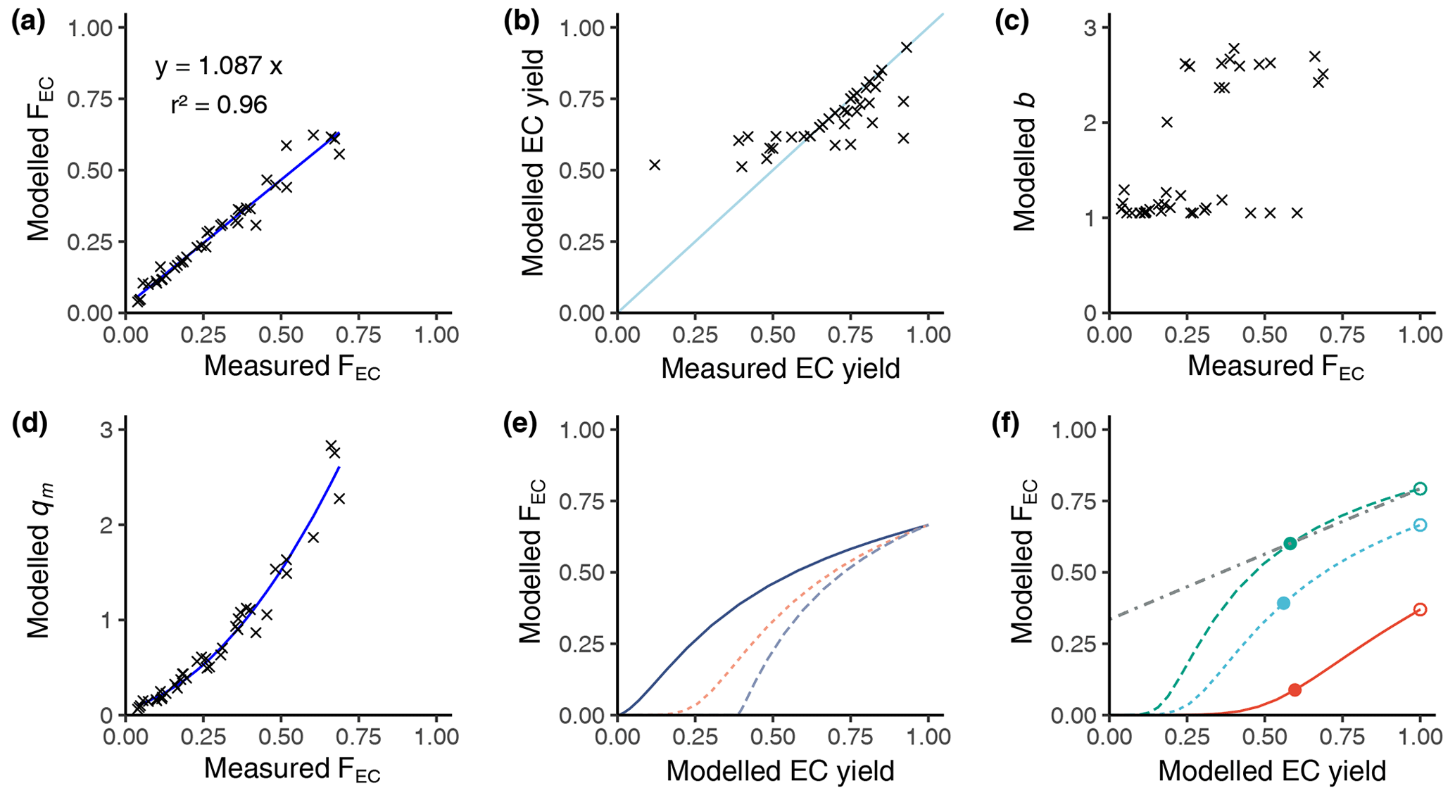
Figure 2 Summary of the modelled EC correction to an EC yield of 1. (a) Model accuracy: modelled F_EC vs. measured F_EC. (b) Modelled EC yield vs. measured EC yield according to Zotter et al. (2014) (see text). (c) Model calculated parameters b. (d) Model calculated parameters q_m. (e) General behaviour of F_EC vs. EC yield for different b values (solid line b=1.1, dashed orange line b=1.2, long blue line b=1.5) with a fixed q_m of 1.5. (f) General behaviour of F_EC vs. EC yield for different q_m values (solid line q_m=0.5, dashed green line q_m=1.5, dashed cyan line q_m=2.5) with a fixed b value of 1.2 and a linear model (dash-dotted line) for a sample with extrapolation at an EC yield of 1. Filled dots show the measured value, and the open dots show the value after extrapolation.

Figure 2e provides examples of the modelling of the F_EC vs. the modelled EC yields for different values of the parameter b. The EC yield is decreased by proportionally increasing the temperature of each of the three steps of the WINSOC removal. The model allows us to extrapolate the F_EC value of any sample with a yield lower than 100 % to the F_EC value corresponding to 100 % yield, which defines the correction for EC loss. According to the Arrhenius approach, the model has a non-linear shape which may be approximated by a linear model in the region of EC yields higher than 0.5. Before developing this non-linear model, we applied a simple linear model for the EC loss correction according to previous publications (Zotter et al., 2014). The measurement conditions usually keep the EC yield higher than 0.4; thus the linear model remains useful under certain conditions. Nevertheless, the non-linear model is superior and shall be used in future. Figure 2f is similar to Fig. 2e but for different q_m values. As shown in Zotter et al. (2014), different samples may show different slopes and intercepts for the linear model. Figure 2e and f show that different values of b and q_m explain the different slopes and intercepts observed previously in the data. Extrapolation and correction to F_EC(corr) of the data from Zotter et al. (2014) are shown in Fig. S6. In Fig. S6, same-colour results belong to punches from the same filter; however the experimental conditions of their online ${}^{\mathrm{14}}\mathrm{C}\left(\mathrm{TC}\right){/}^{\mathrm{14}}\mathrm{C}\left(\mathrm{EC}\right)$ measurements were variated in order to obtain different yields and F_EC values. Therefore, the same-colour results in Fig. S6, ideally, should have the same F_EC value extrapolated to 100 % yield. As indicated in Sect. 2.9, these data were useful to optimise the E_a and K(T_ref) values by minimising the differences between the yield-corrected F_EC of the same-colour results. This optimisation was performed prior to the application of the non-linear model to the results of this paper.

For validation of the correction method for ¹⁴C(EC) presented here, the use of reference material could offer a means. Reference materials were not measured, however, as most of those that are provided are in powder form only (Baumgardner et al., 2012). This powder must be dispersed homogeneously on a filter first, which is difficult to achieve and usually leads to inhomogeneities, which even worsens if water extraction is employed on this dispersed powder. Furthermore, such reference materials (e.g. NIST SRM 1649a) typically contain a certain fraction of coarse particles of up to 100 µm, which is substantially larger than the PM₁₀ size cut from the field samples. According to our experience, coarse particles differ in the $\mathrm{OC}/\mathrm{EC}$ separation and charring behaviour from field samples collected with a PM₁₀ size cut or smaller. To our knowledge, only one reference material exists that is provided on quartz fibre filters, which is NIST SRM 8785 (i.e. SRM 1649a dispersed on filter material using a PM_2.5 size cut). However, the intercomparison study of Szidat et al. (2013) with this reference material showed inhomogeneities that were caused in the dispersion process. Due to this situation, method validation may still be more effective today if based on thoroughly analysed and well-homogenised high-volume filters. Additionally, employing or omitting water extraction is crucial for an agreement between individual labs even when applying different EC isolation techniques. Most participants in the aerosol intercomparison study from Szidat et al. (2013) did not employ water extraction, which resulted in a larger scatter compared to Zenker et al. (2017), where all participants used water extraction to reduce charring. Nevertheless, as no suitable reference material exists, the validation of this method is currently not possible, and therefore it cannot be considered fully validated.

3.2 Concentrations of carbonaceous aerosols

Results from the 21-month sampling period (Table 1) showed a mean TC concentration of 137 ng C m⁻³ (range: 65–264 ng C m⁻³) and a mean EC concentration of 14 ng C m⁻³ (range: 3–40 ng C m⁻³), resulting in a mean $\mathrm{OC}/\mathrm{EC}$ ratio of 11.7 (range: 4.5–27). The filters sampled from 28 September to 6 October 2017 had elevated TC (601 ng m⁻³) and EC (52 ng C m⁻³) levels and were excluded from the mean reported above as this would clearly distort the mean. The $\mathrm{OC}/\mathrm{EC}$ ratio for this filter sample was 10.5 and thus comparable to the mean of the other samples. For 5 of the 13 samples, 2 consecutive filter samples were pooled to obtain a sufficient carbon amount for ¹⁴C analysis (see Table 1). Lower TC values were seen in winter (November to March) compared to summer (April to October), whereas it was the other way around for EC. Consequently, the $\mathrm{OC}/\mathrm{EC}$ ratio shows a seasonality with lower values in winter and higher values in summer. TC on back filters had a mean concentration of 22 ng C m⁻³ (range: 12–49 ng C m⁻³) and showed no seasonality. The mean pure WINSOC concentration (Table 2), corresponding to step 1 of the Swiss_3S protocol, was 26 ng C m⁻³ (range: 9–71 ng C m⁻³), whereas the mixed (WINSOC + EC) S2 and S3 fractions had mean concentrations of 4 ng C m⁻³ (range: 0.5–26 ng C m⁻³) and 7 ng C m⁻³ (range: 1.5–16 ng C m⁻³). The aforementioned high-loading filter sample values from the transition September–October 2017 (111 ng C m⁻³, S1; 26 ng C m⁻³, S2; and 27 ng C m⁻³, S3) were excluded from the mean. The total amount of WINSOC including EC loss was 37 ng C m⁻³ (range: 1.5–16 ng C m⁻³; excluded filter: 164 ng C m⁻³). WSOC was calculated by subtracting EC and total WINSOC from TC, which gave a mean of 39 ng C m⁻³ (range: 0.5–92 ng C m⁻³). The September–October 2017 filter sample had a loading of 284 ng C m⁻³ and was excluded from the mean. The mean amount corrected for charring and EC loss calculated with Sunset-calc (see Sect. 2.11, Table S4) for WINSOC was 34 ng C m⁻³ (range: 11–90 ng C m⁻³; excluded filter: 151 ng C m⁻³), and the mean amount corrected for EC was 15 ng C m⁻³ (range: 3.7–39 ng C m⁻³; excluded filter: 67 ng C m⁻³). For these calculations and corrections, the R Shiny application Sunset-calc was necessary as they were not possible with the default software tools provided for the Sunset $\mathrm{OC}/\mathrm{EC}$ analyser. The ¹⁴C(TC) measurements on back filters (see Table 3) revealed a mean filter loading of 90 ng C m⁻³ (range: 26–189 ng C m⁻³) excluding the autumn 2017 filter, which had a back filter loading of 501 ng C m⁻³.

Table 1 $\mathrm{OC}/\mathrm{EC}$ ratios and filter loadings measured by NILU using the EUSAAR_2 protocol. Filters that were pooled for ¹⁴C analysis are marked with an asterisk.

^* Pooled filters.

Table 2 WINSOC amounts for each step of the Swiss_3S protocol measured at the University of Bern and corresponding WSOC amounts. Fraction S1 is considered pure WINSOC, whereas S2 and S3 are mixed fractions of WINSOC and EC. WSOC was determined by subtraction of EC and total WINSOC from TC.

^* Pooled filters.

Table 3 Filter loadings and fractions for front and back filters for TC measured at the University of Bern.

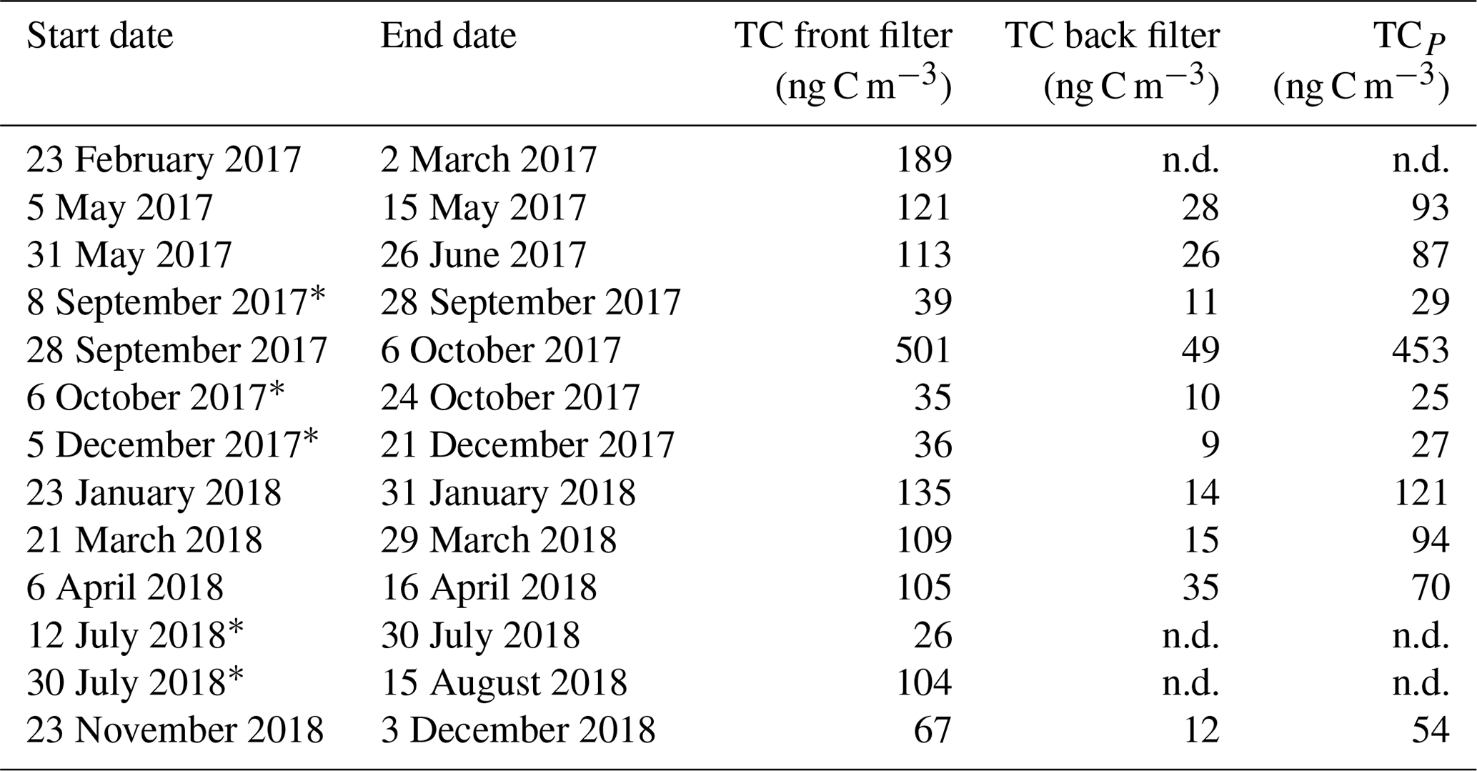
^* Pooled filters. n.d.: not determined.

3.3 Development of preparation methods

3.3.1 Water extraction

For water extraction, three filter punches were stacked to maximise the amount of extractable WSOC. Prior to filter sample extraction, trials with empty filters and the screw type polycarbonate water extraction unit were made. Stacking more than three filters was not feasible, as it makes the water extraction housing prone to leakage. The sample water extraction was gravity-fed. Ultrapure water was filled in the pre-combusted glass syringe directly from the tap of the ultrapure water system and screwed onto the previously assembled water extraction unit to avoid unnecessary liquid transfer. The extraction of 5 mL took 2–3 min depending on the number of filters stacked.

The water-extracted filter material was subjected to WINSOC removal and ¹⁴C(EC) measurement. Elimination of WSOC is beneficial as it is shown to pyrolyse into EC (charring) when subjected to thermal–optical analysis (Yu et al., 2002; Cadle et al., 1980). The F¹⁴C(OC) is generally higher than for F¹⁴C(EC) (Szidat et al., 2004b, 2009; Zhang et al., 2012) but is often exceeded by F¹⁴C(WSOC) due to substantial contributions from biogenic sources and biomass-burning emissions (Zhang et al., 2014a; Kirillova et al., 2013; Weber et al., 2007). Therefore, a small contribution of charred OC significantly biases the measured F¹⁴C of the EC fraction, which is prevented by the WSOC removal.

3.3.2 Adaptations of the OC $/$ EC analyser for WINSOC removal

The filter holders for water extraction are of screw type; thus round punches were required for water extraction. For WINSOC removal, a single layer of filter material cannot exceed the area (1.5 cm²) of the sample holder spoon in the Sunset $\mathrm{OC}/\mathrm{EC}$ analyser. Although it is not necessary to fully cover the sample holder area, the filter cut should cover most of the area to utilise the laser transmission signal for calculations. Stacking of filters should be avoided, as lower filters may not encounter the same conditions as the topmost filter, especially in terms of oxygen supply, which may cause differences with respect to both charring and EC losses within the stack. Furthermore, calculating an EC yield is not feasible after stacking two or more filters. We observed spikes in the laser transmission signal for small filter punches (<0.5 cm²), possibly due to filter movements caused by instrument vibrations. Due to the limitation of circular cuts for water extraction and a rectangular sample holder in the $\mathrm{OC}/\mathrm{EC}$ analyser, the water-extracted filter was cut in quadrants. This enables the complete use of filter material; however, at the expense of a more labour-intensive WINSOC removal. The three water-extracted punches from each filter were cut into 12 and 24 quadrants for each individual and pooled sample, respectively. WINSOC was then removed from each sector using the Swiss_3S protocol (Zhang et al., 2012), requiring 18.5 min per run. High EC losses were observed with the standard Swiss_3S protocol; hence the protocol was adapted. Decreasing the temperature from 450 to 425 ^∘C in S2 and from 650 to 600 ^∘C in S3 increased EC yields from <0.4 to 0.6. Shortening the 600 ^∘C pure He step in S3 from 180 to 120 s, further reduced EC losses, leading to a mean EC yield of 0.87 (range: 0.72–0.95) (Figs. 3 and 4). As shown in Fig. 4, the average charring after WINSOC removal was 2.8 % (range of 1 %–6.8 %) for S1, 0.6 % (0 %–2.4 %) for S2, and 3 % (1.3 %–9.0 %) for S3, with a total charring of 6.5 % (2.5 %–12.9 %). The OC and EC concentrations must be corrected for charring and EC losses using Sunset-calc (see Sects. 2.11 and 3.2). This enables a simple WINSOC removal protocol optimisation and adaptation after each run. The outcome of Sunset-calc is also employed for the correction of biases of ¹⁴C(EC) results caused by charring and EC losses (see Sect. 3.4.1).

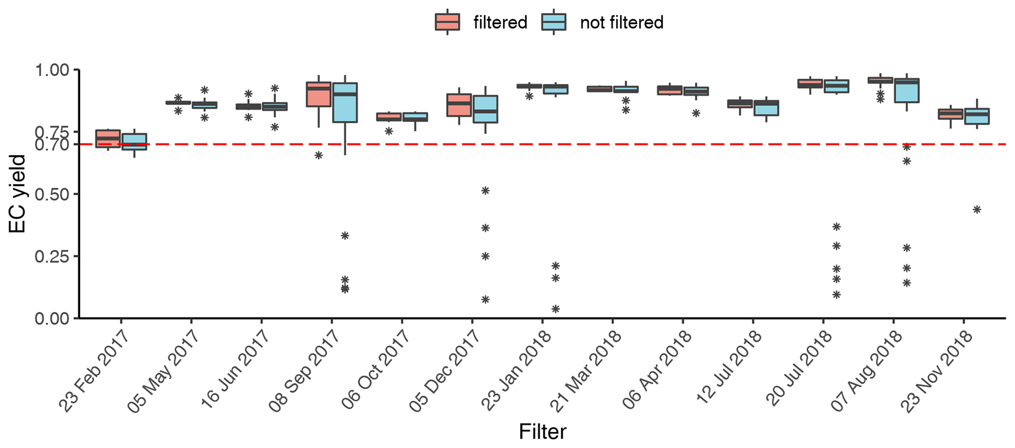
Figure 3 EC yield after WINSOC removal for each filter with the sampling start date. Filtered (WINSOC removal containing outliers in EC yield, fraction of charring S1, S2, or S3 removed) and unfiltered EC yields for each filter are shown. The boxplot box shows the first and third quartiles with the mean as a thick horizontal line for the individual groups (filtered and not filtered). The values outside the 1.5 interquartile range are shown with an asterisk. The horizontal line at 0.7 shows that at least 70 % of the initial EC has been recovered.

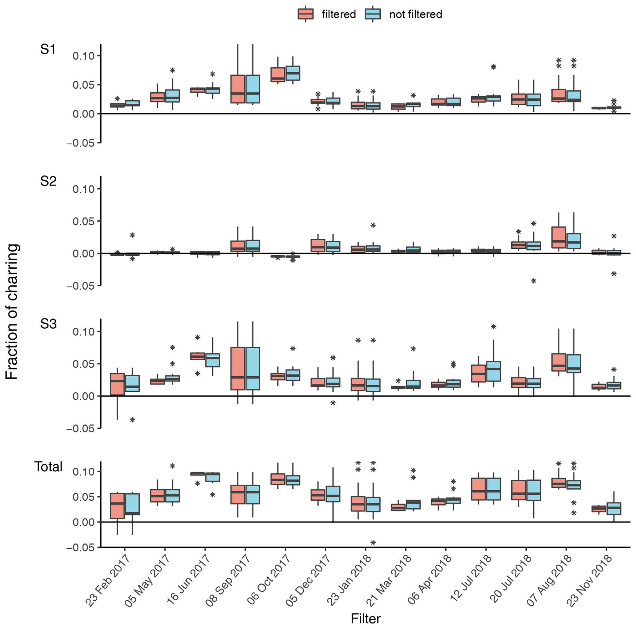
Figure 4 Fraction of charring observed for each filter at the individual steps (S1, S2, S3) and the total (sum of S1, S2, S3) with the sampling start date. Filtered (WINSOC removal containing outliers in EC yield, fraction of charring S1, S2, or S3 removed) and unfiltered fractions of charring for each filter are shown. The fraction of charring describes the amount of artificially produced EC by charring OC related to the amount of EC on the filter based on the laser transmission signal; i.e. a total charring of 0.05 means a 5 % contamination of the total EC amount.

In the present work, WINSOC was removed but not subjected to radiocarbon measurement due to the very low filter loading. In the Swiss_3S protocol, only the S1 fraction consists of pure WINSOC, as S2 and S3 are considered a mixture of WINSOC and EC. The average WINSOC loading in S1 was 1.8 µg C cm⁻², ranging from 0.9 to 3.7 µg C cm⁻², whereas radiocarbon measurements require at least 3 µg C. With more highly loaded filters, ¹⁴C(WINSOC) measurements can be implemented in the workflow presented.

3.3.3 Wet oxidation and WSOC measurement

Filter extraction and chemical wet oxidation may add contaminants, and stringent preparations (Sect. 2.5) were needed to ensure low procedural blanks. This included the use of acid-cleaned (high-purity-grade H₃PO₄) and baked-out glassware and pre-oxidation of the oxidiser solution used to remove contaminants. The freshly prepared oxidiser solution was pre-oxidised at 90 ^∘C for 30 min before helium flushing with helium to remove carbonaceous contaminants. This step removes contaminants in the oxidiser itself as well as in the ultrapure water and equipment used. The oxidiser concentration was increased to 10 % from 4 %, whereas the amount of oxidiser added to the sample was reduced to 0.25 mL from 1 mL, compared to Lang et al. (2012). Oxidation was performed at 75 ^∘C overnight, deviating from previous studies by Lang et al. (2012) (100 ^∘C for 60 min) and Lang et al. (2013) (90 ^∘C for 30 min). EXETAINER^® vials store gas with little leakage even after multiple needle punctures (Glatzel and Well, 2008). All vials used for samples, standards, and blanks were leak-tested before use (Sect. 2.8) at the same temperature (75 ^∘C) as the oxidation step takes place. Vials are more prone to leakage at higher temperatures; hence we lowered the reaction temperature to 75 ^∘C. Both leak testing and a lower reaction temperature kept loss of precious sample material at a minimum. The sample acidification, helium flushing, and chemical wet oxidation were performed the day before measurement. The butyl rubber septum of the EXETAINER^® may contaminate the sample over time when exposed to the strongly acidic and oxidative environment. As a cautionary principle, samples should be measured the day after preparation to minimise any losses, contaminations, and potential isotopic fractionation. In the present work, helium was purged at 75 ^∘C with the gas needle through the oxidised sample, unlike in Lang et al. (2012), where only the headspace was sampled at room temperature. Considerable amounts of liquid (∼0.3 mL per sample) that were carried with the gas were trapped in a custom-built gas wash bottle (25 mL). Remaining water vapour was removed by a SICAPENT^® trap (P₂O₅ on inert carrier material) to protect the zeolite trap in the gas interface system (GIS). The CO₂ amount was determined by the GIS pressure gauge based on the ideal gas law before dilution with helium and feeding the gas mixture into the ion source of the AMS. This procedure provides an estimation of the amount of WSOC only.

3.3.4 Procedural blank

The WSOC procedural blank was determined by performing the water extraction and wet-oxidation procedure, using pre-baked (2 h, 750 ^∘C) quartz fibre filters (Pallflex^® Tissuquartz 2500QAT-UP), as described in Sect. 2.3. After extraction, different amounts of OxII (SRM 4990C) or fossil NaAc solutions (∼1000 ppm) were added to the vials and subjected to chemical wet oxidation (Sect. 2.4). The mass and fraction modern of the contaminant were determined based on the constant-contamination approach by a drift model (Hanke et al., 2017; Salazar et al., 2015) (see Fig. S7). In previous studies, the WSOC eluate was dehydrated by lyophilisation before re-dissolving and combustion in an elemental analyser coupled to an AMS (Zhang et al., 2014a). Compared to the lyophilisation method, the procedural blank was lower for chemical wet oxidation, with a mass of contamination of 0.9±0.2 µg C and the corresponding F¹⁴C of 0.20±0.08.

3.4 Radiocarbon results

3.4.1 Correction of the ¹⁴C(EC) results

Early approaches of ¹⁴C(EC) measurements focused on the separation of OC and EC (Zhang et al., 2012; Barrett et al., 2015; Zencak et al., 2007); however, some OC pyrolyses into EC, creating a positive artefact, and some EC is lost by desorption, degradation, or oxidation (Cadle et al., 1980; Yu et al., 2002; Gundel et al., 1984; Zhang et al., 2012), but efforts to correct ¹⁴C(EC) were not considered then (Szidat et al., 2006, 2004b, a; Dusek et al., 2014; Andersson et al., 2011; Bernardoni et al., 2013). Zhang et al. (2012) implemented a linear correction for EC losses to account for the underestimation of biomass-burning EC. The composition of OC and EC underlies spatial and temporal variability, and thus the linear correction slope will differ. Zotter et al. (2014) addressed this issue by introducing different slopes for winter and summer, as the linear correction slope for EC differs considerably between these two seasons. Consequently, the linear correction slope must be either established for each site with multiple EC yield measurements or estimated based on previous measurements.

For low-loaded filters and for sites with limited filter availability such as the Arctic, linear slope correction with multiple EC yield measurements can be a particular challenge. Here, we apply an optimised approach, using COMPYCALC that combines the determination of both EC losses and EC bias from charring of OC with the thermal-desorption model (Sect. 2.10). Furthermore, COMPYCALC uses the basis of Zhang et al. (2012) for the EC yield calculation and the charring calculation, where the attenuation (ATN, Sect. 2.10) calculated from the laser transmission signal is used. Charring correction after EC yield extrapolation was performed in accordance with Zotter et al. (2014), assuming that half of the pyrolytic EC that forms during the analysis is lost by the last heating step during WINSOC removal, complemented by a correction that considers different sensitivities of the ATN determination towards PC and EC; see Eqs. (10) and (11) in Sect. 2.10. Table 4 summarises EC and OC before and after corrections for EC yield and charring. The initial F¹⁴C(OC) value (F_OC) is calculated with the initial EC value (F_EC) for correction. As described in Sect. 2.10, the COMPYCALC script is run for the extrapolation of EC yield and charring correction to yield the final corrected EC value (F_EC(final)). Then, using F_EC(final), the final OC value (F_OC(final)) is calculated.

Table 4 Radiocarbon values for EC and OC before (i.e. F_EC and F_OC, respectively) and after the COMPYCALC extrapolation (i.e. F_EC(final) and F_OC(final), respectively).

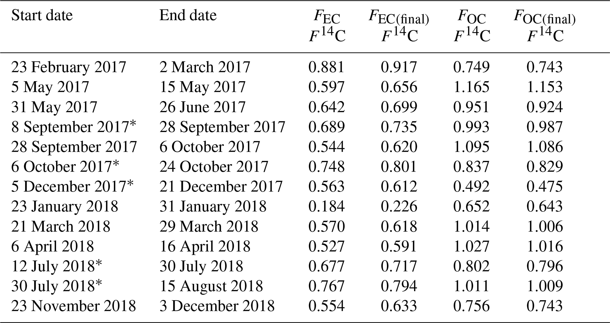
^* Pooled filters.

3.4.2 Quality aspects of the F¹⁴C(OC) calculation

Thermal–optical $\mathrm{OC}/\mathrm{EC}$ separation discussed in the present work focuses on EC and WSOC and the optimisation thereof. Early work on ¹⁴C analysis did not include measures to reduce charring, which included substantial biases in the ¹⁴C analysis, particularly for EC but also for OC, as ¹⁴C(OC) was determined directly by combustion of the filters in oxygen at 340 ^∘C (Szidat et al., 2004b). Later work included water extraction for charring reduction of EC (Yu et al., 2002; Novakov and Corrigan, 1995). Zhang et al. (2012) combined water extraction with an optimised four-step protocol and, thus, further improved $\mathrm{OC}/\mathrm{EC}$ separation. However, only S1 was considered pure OC in this first TOA protocol and thus may include two possible biases of the ¹⁴C(OC) result, as different OC fractions were not considered: first, the portion of OC that undergoes charring in S1 and, thus, is shifted to later steps and, second, more refractory OC that evolves during S2 and S3. This flaw was improved later by Zhang et al. (2015) by omitting the direct ¹⁴C measurement of OC, calculating F¹⁴C(OC) as the difference between F¹⁴C(TC) and F¹⁴C(EC), as it is in the present study (Eq. 7). Hence, a better $\mathrm{OC}/\mathrm{EC}$ separation improves both the quality of the measured F¹⁴C(EC) value and the calculated F¹⁴C(OC) value.

3.4.3 Measurement limitations

Radiocarbon measurement requires a minimum of 2–3 µg C per sample disregarding the hyphenation method (Wacker et al., 2013). With the setup used in the present work, the water extraction method is limited by extraction setup diameter and the number of punches to be stacked. Accordingly, for WSOC a minimum filter loading of 0.3 µg C cm⁻² is required. Within reason, there is no known limit for the chemical wet oxidation. Radiocarbon measurements coupled with the Sunset $\mathrm{OC}/\mathrm{EC}$ analyser are limited by the sample holder, allowing for stacking of up to six rectangular 1.5 cm² filter punches (9 cm² in total). In the present work, the remains after punching out the circular filters for WSOC were used for TC, which makes it difficult to fit the material on the regular sample holder. For pooled samples, the filter area used for TC was 10.4 cm², slightly exceeding the 9 cm² limit. Therefore, for TC combustion we used a custom-built quartz spoon, on which up to 16 cm² of filter material can be placed and combusted. Filter stacking must be omitted for ¹⁴C(WINSOC) measurement. For this reason, filter loadings for S1 (pure WINSOC) of the Swiss_4S protocol must be >2 µg C cm⁻². The ¹⁴C(WINSOC) measurements were omitted in the current study, as only 4 of the 13 samples had a filter loading >2 µg C cm⁻², with a mean loading of 1.8 µg C cm⁻² (range: 0.9–5 µg C cm⁻²).

3.4.4 Radiocarbon results

Radiocarbon measurements of TC show a larger input from fossil carbon in winter months relative to the summer months with an average F¹⁴C of 0.85±0.17 (Table 5). F¹⁴C values close to non-fossil levels of radiocarbon were found for spring, summer, and autumn with an average F¹⁴C of 0.95±0.09 and the highest levels in spring and late summer. Large variations in ¹⁴C(EC) were observed, ranging from 0.23 to 0.92 (mean: 0.66±0.16). Both the highest and the lowest value were observed in winter (23 February–2 March 2017 and 23–31 January 2018), showing that the relative source composition of Arctic carbonaceous aerosol can vary widely within a season. The highest ¹⁴C(EC) value had the second-highest EC concentration (40 ng C m⁻³) and an $\mathrm{OC}/\mathrm{EC}$ ratio of 5.4, whereas the sample with the very low fraction modern carbon had an EC concentration of 16 ng C m⁻³ and $\mathrm{OC}/\mathrm{EC}$ ratio of 9.6. Notably, the ¹⁴C(WSOC) content of the high fraction modern carbon sample (1.077) was substantially higher than that of EC, indicating different sources of WSOC and EC. Overall, ¹⁴C(WSOC) values showed non-fossil levels of radiocarbon with maxima in spring and late summer and lower values in early summer and winter.

Table 5 Final radiocarbon results for each fraction after all calculations and corrections described in this work.

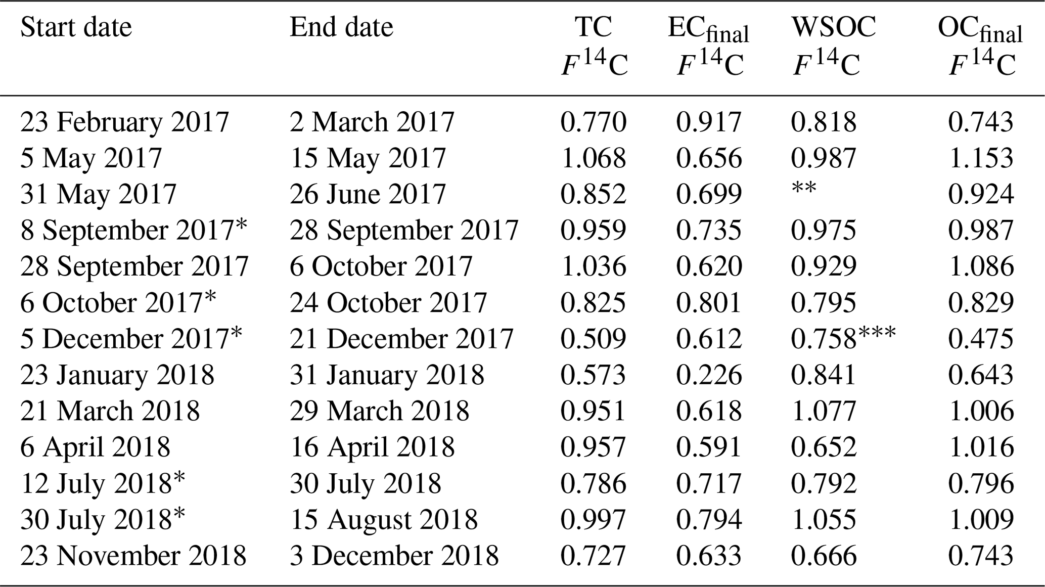
^* Pooled filters.
${}^{**}$ Not measurable due to too low WSOC amount.
${}^{***}$ Only one of the pooled samples (i.e. 5–13 December 2017) was considered as the other one (i.e. 13–21 December 2017) was not measurable due to too low WSOC amount.

Some ¹⁴C measurements of EC have already been performed at the Zeppelin Observatory. Winiger et al. (2015) investigated 14 winter samples from January–March 2009 and observed an average fraction of biomass burning (f_bb) of 0.60±0.21. Later, Winiger et al. (2019) analysed 11 samples from late 2012 to late 2013, which can be classified into 6 winter samples from November 2012 to March 2013 as well as November to December 2013 and 3 summer samples from April to early November 2013. Whereas the winter samples showed f_bb values of 0.37±0.03, indicating a much higher fossil contribution compared to their results from 4 years before and a small variability between the samples, the summer samples revealed a larger scatter with f_bb values of 0.54±0.11. In order to compare our measurement with these two studies, we converted ¹⁴C(EC) results into f_bb values using conversion factors of 1.084 and 1.080 for 2017 and 2018, respectively, based on the approach described in Zotter et al. (2014), providing 0.59±0.24 and 0.63±0.06 for winter and summer, respectively. Our values for summer (i.e. April–October) correspond very well with the summer data from 2013 by Winiger et al. (2019). For the winter data, our results from November to March compare well with the measurements for 2009 from Winiger et al. (2015), whereas there is a large discrepancy of the dataset from 2012/13 from Winiger et al. (2019) with both our outcome and the study of Winiger et al. (2015). This comparison suggests that two substantial changes have occurred from 2009 to 2012/2013 from wood-burning-dominated to fossil-fuel-combustion-dominated EC sources and from 2012/13 to 2017–2018 back to wood-burning-dominated emissions. The discussion and interpretation of this result are beyond the scope of this work. We nevertheless emphasise that the EC isolation procedure of Winiger et al. (2015, 2019) neither involved water extraction nor applied oxygen in the OC removal steps, so these datasets should be compared with caution with our results.

4 Conclusions

In the current study, we present an optimised separation procedure for radiocarbon measurements of TC, EC, and WSOC. Prior to thermal–optical $\mathrm{OC}/\mathrm{EC}$ separation, a water extraction step was used to minimise charring and to provide eluates for ¹⁴C(WSOC) measurement. Our method enables radiocarbon source apportionment of the EC and WSOC fraction in addition to TC and, when sufficiently loaded filters are available, also the WINSOC fraction. Furthermore, the fraction modern of the OC can be calculated from these values. Prior to AMS ¹⁴C analysis, combustion of TC, EC, and WINSOC are all performed with a Sunset $\mathrm{OC}/\mathrm{EC}$ analyser, simplifying the measurement by using a single hyphenation device for multiple carbonaceous fractions. Lacking standard reference material for atmospheric EC on filters, we chose thoroughly analysed and well-homogenised high-volume filters for method validation. As demonstrated for low-loaded Arctic filters, chemical wet oxidation is a simple and reliable method for measurement of the WSOC fraction, providing low procedural blanks. Intercomparison with other methodologies is pending. Furthermore, complete method validation is not feasible due to the unavailability of suitable reference material. Due to this situation, method validation may still be more effective today if based on thoroughly analysed and well-homogenised high-volume filters.

We have developed a web tool for calculation of both amount and EC yield, named Sunset-calc, allowing an EC yield calculation after each run and providing the fraction of charring for each step in the Swiss_3S protocol. Sunset-calc enables rapid protocol optimisations for a low fraction of charring while avoiding too large EC losses before the S4 step.

Our thermal-desorption model approach for EC yield extrapolation provides a filter-specific non-linear correction based on the underlying physical properties of the $\mathrm{OC}/\mathrm{EC}$ mixture and OC composition. The present method is a major leap forward in ¹⁴C(EC) correction calculation and supersedes the currently used linear approach for EC yield extrapolation. Radiocarbon measurements using filters with deliberately lowered EC yields are no longer necessary. Our approach is independent of season and does not require additional filter material for EC yield extrapolation, which is crucial when only limited amounts of sample material are available.