Understanding the potential of Sentinel-2 for monitoring methane point emissions

The use of satellite instruments to detect and quantify methane emissions from fossil fuel production activities is highly beneficial to support climate change mitigation. Different hyperspectral and multispectral satellite sensors have recently shown potential to detect and quantify point-source emissions from space. The Sentinel-2 (S2) mission, despite its limited spectral design, supports the detection of large emissions with global coverage and high revisit frequency thanks to coarse spectral coverage of methane absorption lines in the shortwave infrared. Validation of S2 methane retrieval algorithms is instrumental in accelerating the development of a systematic and global monitoring system for methane point sources. Here, we develop a benchmarking framework for such validation. We first develop a methodology to generate simulated S2 datasets including methane point-source plumes. These benchmark datasets have been created for scenes in three oil and gas basins (Hassi Messaoud, Algeria; Korpeje, Turkmenistan; Permian Basin, USA) under different scene heterogeneity conditions and for simulated methane plumes with different spatial distributions. We use the simulated methane plumes to validate the retrieval for different flux rate levels and define a minimum detection threshold for each case study. The results suggest that for homogeneous and temporally invariant surfaces, the detection limit of the proposed S2 methane retrieval ranges from 1000 to 2000 kg h⁻¹, whereas for areas with large surface heterogeneity and temporal variations, the retrieval can only detect plumes in excess of 500 kg h⁻¹. The different sources of uncertainty in the flux rate estimates have also been examined. Dominant quantification errors are either wind-related or plume mask-related, depending on the surface type. Uncertainty in wind speed, both in the 10 m wind (U₁₀) and in mapping U₁₀ to the effective wind (U_eff) driving plume transport, is the dominant source of error for quantifying individual plumes in homogeneous scenes. For heterogeneous and temporally variant scenes, the surface structure underlying the methane plume affects the plume masking and can become a dominant source of uncertainty.

1 Introduction

Methane (CH₄) is the second most important anthropogenic greenhouse gas after carbon dioxide (CO₂). Its global warming potential is 86 times that of CO₂ over 20 years, and it has a relatively short lifetime in the atmosphere (9 ± 1 years) (Etminan et al., 2016). Fossil fuel production activities represent between 30 % and 42 % of the total global anthropogenic emissions (Saunois et al., 2020). These emissions come from oil and gas (O&G) production infrastructure (e.g., wells, compressor stations) (Lyon et al., 2016) and coal mines. The facility typically emits a gas plume of highly concentrated methane from a small source area (referred to as “point emissions”) (Duren et al., 2019). The mitigation of a large fraction of these emissions is technically feasible and cost effective and represents a key means to reduce the amount of greenhouse gases in the atmosphere (CCAC, 2021; IPCC, 2021).

Satellites measuring backscattered solar radiation in the short-wave infrared (SWIR) spectral region can detect subtle signal variations linked to methane absorption (Jacob et al., 2022). Area flux mappers such as GOSAT and TROPOMI provide daily mapping of methane concentrations at a large spatial scale (Qu et al., 2021). This provides long-term methane trends at a global and regional scales, the latter being instrumental in identifying hotspot areas of anthropogenic methane emissions. At a finer spatial resolution (3.7 to 100 m), several studies have demonstrated that point-source imager satellites can identify individual emissions with detection thresholds from 100 to 10 000 kg h⁻¹. For example, Varon et al. (2018) described a set of algorithms to detect and quantify methane point sources focusing on the private GHGSat constellation. More recent studies have shown the feasibility of quantifying methane point sources from hyperspectral and multispectral missions such as PRISMA (Guanter et al., 2021), Sentinel-2 (S2) (Varon et al., 2021), Landsat-8 (Ehret et al., 2022) and WorldView-3 (Sánchez-García et al., 2022). These recent advances have revealed the existence of large point emissions from O&G production regions (Irakulis-Loitxate et al., 2021, 2022b), coal carbon mines (Guanter et al., 2021) and O&G offshore platforms (Irakulis-Loitxate et al., 2022a).

Hyperspectral satellite imagery (e.g., PRISMA) is capable of resolving fine methane absorption features in the SWIR and typically provides a detection limit from roughly 100 to 500 kg h⁻¹ (Jacob et al., 2022). However, current hyperspectral missions have a low revisit frequency that limits their usefulness for monitoring on a global scale. By contrast, the S2 and Landsat missions provide a unique combination of global coverage, detailed instrument characterization and a 5 d temporal revisit (Gascon et al., 2017; ESA, 2022; Micijevic et al., 2022), but the sensitivity of their coarse SWIR bands to methane absorption is limited, so that expected detection thresholds can be slightly over 2000 kg h⁻¹ as first suggested by Varon et al. (2021) or slightly lower (at 1800 kg h⁻¹) under favorable conditions as suggested by Irakulis-Loitxate et al. (2022b). The usefulness of the S2 mission for mapping point-source emissions has already been demonstrated at the Korpeje O&G region in Turkmenistan by Varon et al. (2021) and Irakulis-Loitxate et al. (2022b) and at a set of O&G basins across the globe by Ehret et al. (2022).

The development of global and systematic monitoring of methane point sources requires the accurate validation of the retrieval algorithm in different conditions, such as solar illumination, surface heterogeneity or atmospheric composition. These validation exercises can be either based on in situ controlled emissions or simulated analysis. The former approach provides the most accurate benchmark and real conditions but is limited to a small set of data points due to high logistic costs and the negative impact on the atmosphere (Sherwin et al., 2022). The latter approach, despite its challenging reproduction of real scene conditions, can provide validation scenarios of methane point-source emissions for any satellite at a global level.

These simulated approaches can be based on an end-to-end framework that covers the solar irradiance, atmosphere, surface and satellite characteristics (Jongaramrungruang et al., 2021). This is a convenient method to study the sensitivity of different satellite characteristics such as sensor noise or spectral resolution. However, the more subtle specifications of the instrument (e.g., per-pixel viewing dependence) or scene characteristics might be difficult to reproduce. Cusworth et al. (2019) introduced a detailed study of the detection and quantification of methane point sources from several hyperspectral missions based on their spectral and noise characteristics. This alternative approach used simulated methane plumes and incorporated their transmittance into simulated satellite acquisitions. By doing so, the satellite radiance observations were not altered while the plume enhancement was integrated into the scene. We adopt this latter methodology here and refine it in Sect. 3 to account for a compensation term that corrects for the convolution of the methane transmittance signal after its band integration. This error is present for every type of instrument at different levels, but for multispectral missions with a large bandwidth such as S2, a larger impact is expected.

Our simulated datasets validate the retrieval algorithm proposed in Sect. 4 for a set of sites and methane plumes presented in Sect. 2. These plumes represent the temporal evolution of a point source plume with changing spatial distribution. The selected sites are representative of well-known O&G basins with different scene heterogeneity.

The validation process presented in Sect. 6.2 generates several datasets at different flux levels. This methodology validates the methane flux rate at different levels and, at the same time, defines the detection limit of the instrument for a set of sites and methane plumes. Section 6.3 expands this analysis to cover a large number of plumes and different periods of the year. The results highlight several uncertainty contributions associated with the methane flux that we disentangle into different sources in Sect. 6.4.

2 Sentinel-2 data and sites of study

The first satellite unit (S2A) of the S2 mission was launched in 2015 and, together with the second satellite unit S2B launched in 2017, provides continuous monitoring of terrestrial surfaces and coastal waters at a global scale with better than a 5-day revisit. Both satellites carry on-board the Multi-Spectral Instrument (MSI) with 13 spectral bands in the visible and near-infrared (VNIR) and the shortwave infrared (SWIR) at spatial resolutions of 10, 20 or 60 m. Top-of-atmosphere (TOA) reflectance images are delivered to the public after geometric and radiometric calibration (L1C products) Products are free open-access from the Sentinels Scientific Data Hub in a set of ortho-images (in UTM/WGS84 projection) of about 100 × 100 kg h⁻¹ (Gascon et al., 2017).

The bands in the SWIR region, B11 and B12, measure the TOA radiance at an approximate 20 m spatial resolution. Although they were not designed to detect and quantify methane point-source emissions, these two bands are sensitive to methane absorption and have shown that they have the capability to monitor large emissions at a global scale (Varon et al., 2021; Ehret et al., 2022). Figure 1 illustrates the spectral response of bands B11 and B12 for both satellite units together with the methane transmittance for a surface concentration of 1904 ppm and air–mass factor (AMF) of 2.

Figure 1 S2A and S2B spectral response functions of bands B11 and B12 combined with the methane transmittance for a surface concentration of 1904 ppm and AMF of 2.

Both of these bands cover a small spectral region of methane absorption. In the case of B12, it is significantly wider than B11. Despite carrying the same MSI instrument, S2A and S2B do not exactly match the same spectral response. Although the differences are within the specifications, it shows that the S2A B12 is slightly more sensitive to methane absorption as compared to S2B satellite unit.

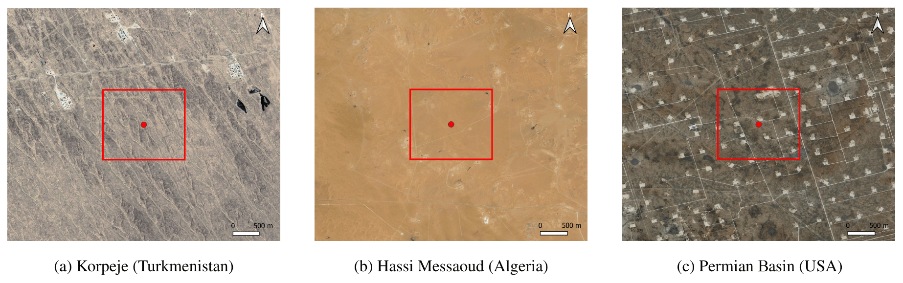
Figure 2 RGB image of the selected areas of (a) Korpeje (Turkmenistan), (b) Hassi Messaoud (Algeria), and (c) Permian Basin (USA). The selected area (red box) corresponds to 1500 × 1500 m² centered at the latitude and longitude 38.493918^∘, 54.216550^∘​​​​​​​ (Korpeje), 31.82652^∘, 6.15011^∘ (Hassi Messaoud), and 31.72070^∘, −102.28663^∘ (Permian Basin). Source map from © Google Earth and © Microsoft Bing.

Figure 2 shows the selected areas of study: Korpeje in Turkmenistan, Hassi Messaoud in Algeria and the Permian Basin in the USA. The specific locations correspond to an area of 1500 × 1500 m² centered at the latitude and longitude 38.493918^∘, 54.216550^∘ (Korpeje), 31.82652^∘, 6.15011^∘ (Hassi Messaoud) and 31.72070^∘, −102.28663^∘​​​​​​​ (Permian Basin).

These areas have been selected (1) for being well-known O&G activity locations, (2) for showing persistent high methane concentrations as observed by TROPOMI for years and (3) because they are well-studied reference sites in the literature (Varon et al., 2019; Zhang et al., 2020; Varon et al., 2021; Cusworth et al., 2021; Guanter et al., 2021; Irakulis-Loitxate et al., 2022b; Lauvaux et al., 2022). In the case of Korpeje, the selected location is near a compressor station with high emission fluxes and frequency but far enough away so that no real plumes contaminate the test images. In Algeria, the Hassi Messaoud oil field is located in a desert area with extremely uniform spatiotemporal conditions. Finally, the location selected in the Permian Basin is characterized by including a high number of wells and pipeline crossings. In addition, the scene might suffer from temporal variations that include atmospheric conditions, vegetation changes or human activities in the area. In the literature, other study areas widely known for high emission rates or high emission potential can be found, such as the Shanxi region in China (Guanter et al., 2021) or the O&G fields in Canada (Chan et al., 2020; Williams et al., 2021; Tyner and Johnson, 2021). However, the high surface heterogeneity and cloud cover throughout the year over these areas limits the application of methane retrieval methods with multispectral instruments with coarse spectral resolution such as S2.

The selected S2 acquisitions for the simulation of methane plumes are the S2A tile 40SBH acquired on 18 July 2021 for the Korpeje site, the S2A tile 32SKA acquired on 2 July 2021 for Hassi Messaoud and the S2A tile 13SGR on 4 July 2021 for the Permian Basin. A temporal normalization selection searches for the closest cloud-free overpass with the same viewing overpass (see Sect. 4). If the closest cloud-free overpass is selected, this will typically correspond to a different satellite unit (due to orbit phase differences between S2A and S2B satellite units) with slightly different spectral responses. Thus, this corresponds to S2B acquisitions on 13 July 2021 (Korpeje), 27 June 2021 (Hassi Messaoud) and 9 July 2021 (Permian Basin).

3 Simulating Sentinel-2 observations of methane plumes

We used the Weather and Research Forecasting Model in large-eddy simulation mode (WRF-LES) to generate realistic methane plumes (three-dimensional mass distributions) in the atmospheric boundary layer over time, following the approach of Varon et al. (2018). The simulation was conducted at 30 × 30 m² spatial resolution with an initial geostrophic wind field of 3.5 m s⁻¹ and a sensible heat flux H=300 W m⁻².

The original resolution of the simulation was resampled to the 20 m spatial resolution of S2. This resampling is performed at each layer of the vertical grid to minimize interpolation error. The simulation is performed under a reference flux that is then scaled linearly to the desired level following Guanter et al. (2021) and Sánchez-García et al. (2022).

The resulting 3-D methane distributions can be vertically integrated in order to obtain a 2D mass field of column mass enhancement ΔΩ in kg m⁻². These maps are further converted into column-averaged dry molar mixing ratio $\mathrm{\Delta }{X}_{{\mathrm{CH}}_{\mathrm{4}}}$ (unitless) maps following the relationship

$$\begin{array}{}\text{(1)}& \mathrm{\Delta }\mathrm{\Omega }={\displaystyle \frac{M_{{\mathrm{CH}}_{\mathrm{4}}}}{M_{\mathrm{a}}}}{\mathrm{\Omega }}_{\mathrm{a}}\mathrm{\Delta }{X}_{{\mathrm{CH}}_{\mathrm{4}}},\end{array}$$

where M_a and $M_{{\mathrm{CH}}_{\mathrm{4}}}$ refer to the molar mass of dry air and methane, respectively (kg mol⁻¹), and Ω_a refers to the column of dry air (kg m⁻²).

Figure 3 Methane enhancement map $\mathrm{\Delta }{X}_{{\mathrm{CH}}_{\mathrm{4}}}$ of the five plumes considered for the simulations scaled at a flux rate Q=1000 kg h⁻¹ after resampling to 20 m resolution.

From the WRF-LES simulations, we selected five different snapshots that were used as representative shapes of methane plumes for the simulations (see Fig. 3).

The methane plume transmittance map as a function of wavelength, T_plume(λ), can be modeled at a fine spectral resolution. Similarly to Cusworth et al. (2019), the spectral optical depth τ(λ) of each atmospheric layer can be described as the multiplication of the HITRAN absorption cross-sections (σ_H; Kochanov et al., 2016), the vertical column density of dry air and the methane volume mixing ratio enhancement (ΔVMR) from the LES.

On the other hand, the resulting map of $\mathrm{\Delta }{X}_{{\mathrm{CH}}_{\mathrm{4}}}$ can be directly converted into T_plume(λ) by using a predefined look-up table (LUT) that establishes the relationship between the two quantities at different AMF values with MODTRAN (Berk et al., 2014). This alternative approach has been proven to produce similar results with a much lower computational cost. Thus, this is the method proposed when a large number of simulations are required and implemented for the datasets in Gorroño et al. (2021).

Once the transmittance of the methane plumes has been calculated, it is convolved with the S2 spectral response to obtain a methane plume transmittance map for each spectral band. This can be directly multiplied with the original S2 TOA radiance maps. This approach has the largest advantage since it reproduces the exact same observation conditions as the original observation. The resulting simulation incorporates a real scene from S2, meaning that effects such as instrument noise or angular pixel dependencies are already included in the simulation. The drawback of this approach is that it becomes mathematically impossible to convolve a signal that corresponds to an already band-integrated quantity. The correct implementation would weight the methane transmittance of each infinitesimal wavelength with the S2 band response. Introducing a weighting afterward, results in an error with respect to the correct implementation that must be considered.

Recent work by Guanter et al. (2021) and Sánchez-García et al. (2022) included a compensation term in the calculated total atmospheric transmittance capable of partially correcting for the bias introduced by this a-posteriori convolution of the methane transmittance for PRISMA and WV-3 simulations, respectively. In those two cases, a simplified approach was selected by considering the total transmittance of the atmosphere T_atm(λ) rather than reconstructing the full TOA radiance. This approach can be sufficient for an instrument that measures in narrow bands where it can be assumed that the surface reflectance and downwelling irradiance are not rapidly changing across them. However, this assumption might not hold for highly heterogeneous surfaces and spectral bands that span through a larger portion of the SWIR spectrum, such as S2 B12 (bandwidth of 180 nm). In that case, it is advisable to include a reconstructed top-of-atmosphere radiance L_TOA in the correction. Here, we will test the implications and their correction by including a term that not only includes the total transmittance but also a reconstructed L_TOA. The corrected L_TOA for the B12 band can be written as

$$\begin{array}{}\text{(2)}& L_{\mathrm{B}\mathrm{12}}^{\mathrm{plume}}=L_{\mathrm{B}\mathrm{12}}\left(\underset{\mathrm{B}\mathrm{12}}{\int }{T}_{\mathrm{plume}}\left(\mathit{\lambda }\right)\mathrm{d}\mathit{\lambda }\right){\mathit{ϵ}}_{\mathrm{convolution}},\end{array}$$

where T_plume indicates the transmittance of the methane plume and ϵ_convolution refers to the bias introduced by the a-posteriori convolution. The term L_B12 corresponds to the original S2 B12 radiance that is integrated at the instrument focal plane as

$$\begin{array}{}\text{(3)}& L_{\mathrm{B}\mathrm{12}}=\underset{\mathrm{B}\mathrm{12}}{\int }{L}_{\mathrm{TOA}}\left(\mathit{\lambda }\right)\mathrm{d}\mathit{\lambda }.\end{array}$$

The correction term ϵ_convolution can be modeled as

$$\begin{array}{}\text{(4)}& {\mathit{ϵ}}_{\mathrm{convolution}}={\displaystyle \frac{{\int }_{\mathrm{B}\mathrm{12}}{L}_{\mathrm{TOA}}\left(\mathit{\lambda }\right)T_{\mathrm{plume}}\left(\mathit{\lambda }\right)\mathrm{d}\mathit{\lambda }}{\left({\int }_{\mathrm{B}\mathrm{12}}{L}_{\mathrm{TOA}}\left(\mathit{\lambda }\right)\mathrm{d}\mathit{\lambda }\right)\left({\int }_{\mathrm{B}\mathrm{12}}{T}_{\mathrm{plume}}\left(\mathit{\lambda }\right)\mathrm{d}\mathit{\lambda }\right)}},\end{array}$$

with the L_TOA(λ) modeled as

$$\begin{array}{}\text{(5)}& L_{\mathrm{TOA}}\left(\mathit{\lambda }\right)=T_{\mathrm{atm}}\left(\mathit{\lambda }\right){\mathit{\rho }}_{\mathrm{surface}}\left(\mathit{\lambda }\right)E_{\mathrm{g}}\left(\mathit{\lambda }\right);\end{array}$$

T_atm refers to the total transmittance through the atmosphere, ρ_surface represents the surface reflectance and E_g is the downwelling irradiance at the ground level. The path radiance and spherical albedo are not considered in this case since their impact in the SWIR region can be considered negligible in the correction.

Combining Eqs. (2) and (4), the term ∫_B12T_plume(λ)dλ is canceled, and we can also reconsider the equation as a simulated plume transmittance convolved with a simulated hyperspectral TOA radiance.

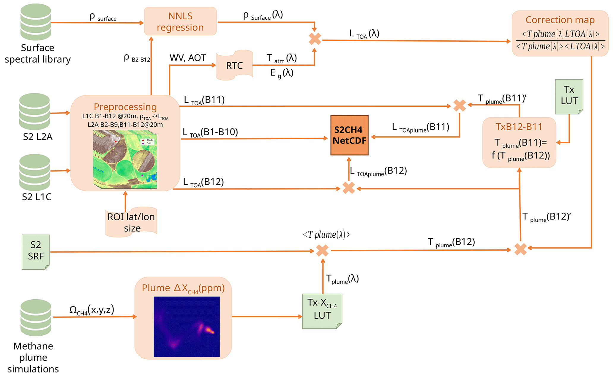
Figure 4 Flow diagram describing the process to generate S2 datasets with embedded methane plume simulations. The diagram contains Copernicus Sentinel-2 images provided by ESA.

This mathematical framework has been implemented in a software capable of producing S2 datasets with simulated methane plumes (Gorroño et al., 2021). Its flow diagram is presented in Fig. 4.

The lower part of the diagram describes the calculation of the methane plume transmittance. The software implementation simplifies the process by only considering the S2 B12 band. The impact over the rest of the bands can be considered negligible except for the B11. At this spectral region, there is a smaller area of methane absorption that must be correctly captured in the simulation. Rather than a direct calculation, it was found that a pre-compiled relationship between the methane plume transmittance of B12 and B11 was more efficient. Using the radiative transfer software MODTRAN (Berk et al., 2014), we generated different methane transmittances at different concentration values. Further convolution of the transmittance by the B11 and B12 spectral response established the mathematical dependency.

The upper part of Fig. 4 captures the calculation process of L_TOA. This requires the processing of the S2 L2A product and obtains the values for surface reflectance, water vapor and AOT. The latter two are used to parameterize a radiative transfer model based on Libradtran (Emde et al., 2016; Mayer and Kylling, 2005) that results in an estimated total transmittance through the atmosphere T_atm and downwelling irradiance E_g. Although the simulation can be performed at a pixel level, to reduce the computational cost, the radiative transfer is only run for a mean value over the area of interest under the assumption that atmospheric variations are small in the vicinity area. The surface reflectance for each S2 band is combined with a set of spectral signatures from the USGS speclib (Kokaly et al., 2017). A non-negative linear regression (NNLS) estimates the hyperspectral surface reflectance.

4 Retrieval methodology

The estimation of methane concentration enhancement is typically based on the fitting of high-spectral-resolution observations in the SWIR spectral region against a modeled radiance spectrum in a single overpass (Thorpe et al., 2014; Jacob et al., 2016).

For multispectral instruments, the SWIR spectral region cannot be resolved in detail, but it is still possible to retrieve methane concentration enhancements from an estimated methane transmittance image. This methane transmittance is calculated as the ratio between the radiance at a spectral channel affected by methane absorption and a methane-free reference band. Mathematically the plume transmittance can be described as

$$\begin{array}{}\text{(6)}& T_{\mathrm{plume}}\left(\mathit{\lambda }\right)\sim {\displaystyle \frac{L}{L_{\mathrm{ref}}}}=e^{-\mathrm{AMF}\cdot {\mathit{\sigma }}_{{\mathrm{CH}}_{\mathrm{4}}}\cdot \mathrm{\Delta }{X}_{{\mathrm{CH}}_{\mathrm{4}}}},\end{array}$$

where L and L_ref represent the radiance of the methane-sensitive band and the methane-free reference band, respectively. AMF refers to the air–mass factor. The methane concentration enhancement $\mathrm{\Delta }{X}_{{\mathrm{CH}}_{\mathrm{4}}}$ is the quantity of interest and expresses the increment produced by the plume from the background methane present in the atmospheric column.

Thus, the proposed rationale to detect methane plumes for the S2 mission is based on an estimation of the plume transmission defined by the ratio

$$\begin{array}{}\text{(7)}& {\displaystyle \frac{\mathit{\rho }}{{\mathit{\rho }}_{\mathrm{ref}}}}={\displaystyle \frac{{\mathit{\rho }}_{\mathrm{B}\mathrm{12}\mathrm{plume}}/{\mathit{\rho }}_{\mathrm{B}\mathrm{11}\mathrm{plume}}}{{\mathit{\rho }}_{\mathrm{B}\mathrm{12}\mathrm{plumefree}}/{\mathit{\rho }}_{\mathrm{B}\mathrm{11}\mathrm{plumefree}}}},\end{array}$$

where the subscript plume and plumefree refer to the overpasses with methane plume emissions and without it, respectively, and ρ refers to the TOA reflectance.

The methane plume quantification can be obtained by establishing a relationship between the term $\mathrm{\Delta }{X}_{{\mathrm{CH}}_{\mathrm{4}}}$ and T_plume(λ) in Eq. (6). An LUT with the relationship between these two quantities and the methane enhancement is established. This LUT incorporates the small but non-negligible effect of methane absorption in B11. The LUT is a function of the AMF and the radiance ratio proposed in Eq. (7). The transmittance in Eq. (7) was calculated as the ratio of the transmittance between B12 and B11 bands due to different methane concentrations.

In order to test the validity of this approach, the retrieval method was tested on the datasets generated in Sect. 3 (Gorroño et al., 2021). The test has set the temporal normalization against the same observation without plume emission. This cancels the noise of the sensor, and an ideal scenario can be tested. Figure 5 shows the test of such an ideal scenario with plume 2 (see Fig. 3b) and Q of 5000 kg h⁻¹. In the absence of noise, only the linear regression between retrieved and reference methane enhancement pixels is shown. The figure includes a simulation with no correction (i.e., ϵ_convolution=1), another with the correction of the T_atm(λ) and a last one with the L_TOA(λ) correction as explained above.

Figure 5 Linear regression of retrieved pixel values versus reference methane enhancement for the Korpeje site (see Fig. 2a), plume 2 (see Fig. 3b) and Q of 5000 kg h⁻¹. The reference acquisition is the same as the target one with no excess methane to simulate an ideal scenario.

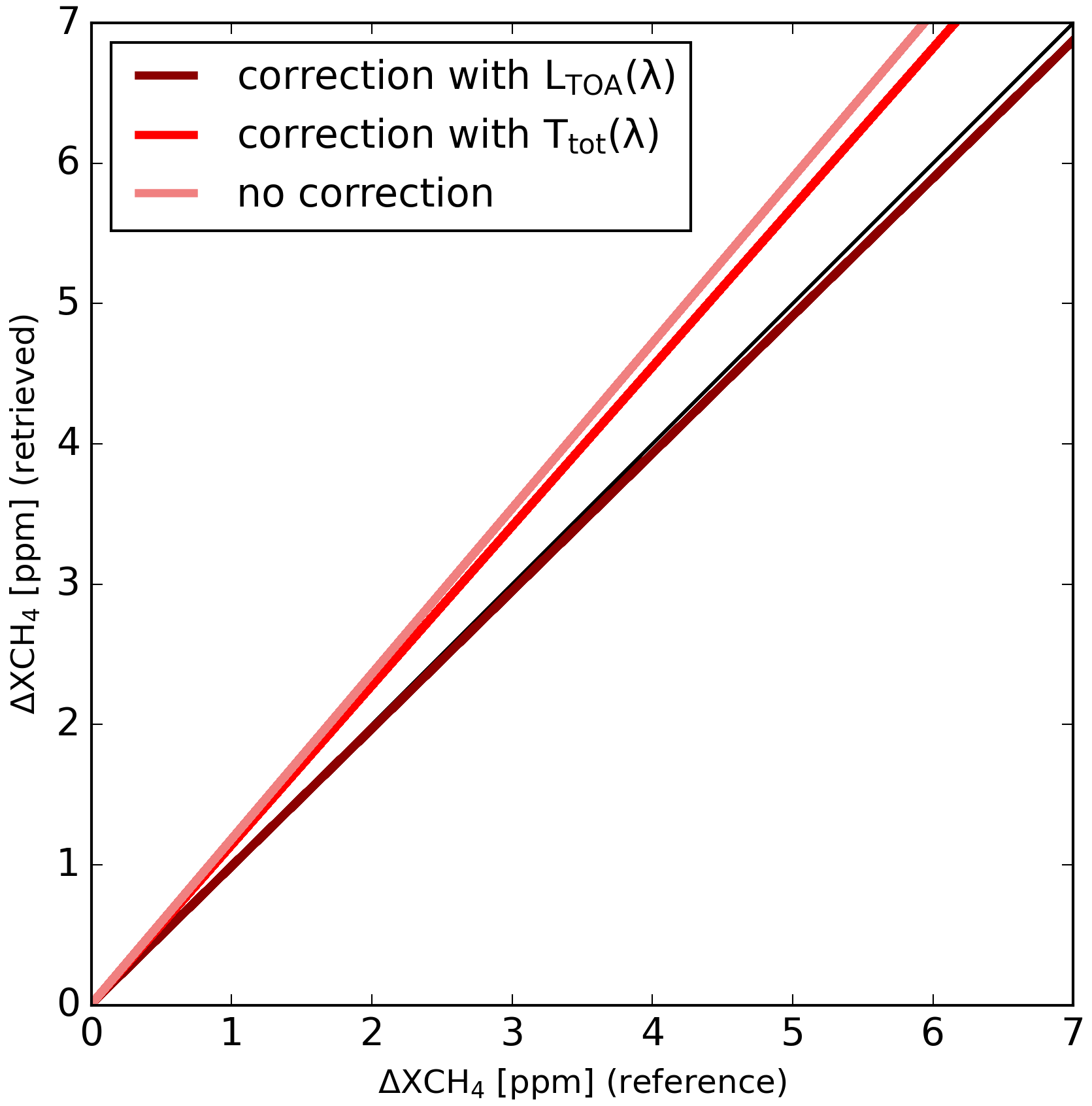
This plot shows that the methodology proposed in Fig. 4 results in simulated datasets with a large agreement. The uncertainty on the methane retrieval algorithm, and especially the flux rate quantification, is expected to be considerably higher. Therefore, the potential uncertainty on the simulated reference (here better than 3 %) will have a negligible impact on the validation. The results also show how the correction methodology largely improves the simulation as compared with no correction applied. From the three elements considered in the TOA model in Eq. (5), the term E_g plays a major role here. The S2 B12 spans from 2100 to 2300 nm, and the downwelling irradiance in this region rapidly decreases with higher wavelengths. Thus, the direct multiplication of the methane transmittance shows an overestimation if no weighting is applied (the S2 B12 band is more sensitive to methane in the 2200–2300 nm region). The term T_atm(λ) improves the correction but at a minor scale similarly to ρ_surface. However, this latter term is scene dependent, and its impact could be considerable for other type of surfaces such as snow at different granule levels.

Once the methane enhancement map has been generated, a median filter with a 3-pixel window is applied for smoothing before the masking process. The standard deviation σ of a region not affected by the methane plume is calculated and the 2σ (95 % confidence interval) is applied as the masking threshold. The selected region for the noise threshold calculation of the plumes in Fig. 3 corresponds to the right-hand area of 300 × 1500 m² out of the plume emission. This masking process is slightly different to the one proposed by Varon et al. (2018) since it applies a median filter before masking rather than masking with the background noise and applying a median filter over the Boolean result. Although this masking process alters the original enhancement map, it is helpful to reduce the significant noise levels present in the S2 methane retrievals, and the resulting mask is applied to the original concentration map. A median filter (or other high-frequency filtering process) is expected to have a low impact on the plume signal since this is distributed in the atmosphere as a low-frequency signal. Nonetheless, this process could remove the signal for very narrow plumes (just one or two pixels' width).

The result of the process is a masked image that flags the potential pixels with a plume emission. The actual plume detection is achieved with an automated cluster detection algorithm based on labels and regionprops methods in the scikit-image Python package (van der Walt et al., 2014), which searches for clusters of at least 40 masked pixels. This is a slightly conservative approach (hereafter referred to as “conservative masking”) since the plume can be detected with a lower threshold if a supervised approach or other techniques are used. Thus, we proposed a second scenario (hereafter referred to “supervised masking”) where the masking threshold and normalization reference observation can be changed and optimized to improve this detection limit. In this second scenario, the number of masked pixels is reduced to 20, and the reference observation can be the average of the two closest acquisitions separated by 5 d. For both Korpeje site (see Fig. 2a) and the Permian Basin (see Fig. 2c), the number of reference observations was not increased. In Korpeje, the average of two products resulted into almost and identical results (the retrieval noise improvement across the scene was lower than 5 ppm) whereas in the Permian one of the closest images was contaminated by clouds. On the contrary, for Hassi Messaoud (see Fig. 2b), the reference observation is the average of 27 June and 7 July 2021 overpasses. The use of these two acquisitions resulted in a scene noise improvement over 20 ppm. By reducing the number of pixels to 20, the masking process might include retrieval artifacts in addition to true methane plumes. By examining the retrieved methane enhancement maps $\mathrm{\Delta }{X}_{{\mathrm{CH}}_{\mathrm{4}}}$, we can manually discard those areas that cannot be attributed to emissions. For example, this was the case for the roads in the Permian Basin (see Fig. 2c) or the O&G facilities close to border of the selected region in Hassi Messaoud (see Fig. 2b).

The method to convert the methane enhancement maps $\mathrm{\Delta }{X}_{{\mathrm{CH}}_{\mathrm{4}}}$ into methane flux rates Q is the integrated mass enhancement (IME) model, which refers to the measure of the total excess mass of observed methane (Frankenberg et al., 2016; Varon et al., 2018). The $\mathrm{\Delta }{X}_{{\mathrm{CH}}_{\mathrm{4}}}$ values are converted from ppm units to kg (Thompson et al., 2016; Duren et al., 2019) by considering the 20 m S2 pixel resolution, the Avogadro's law where 1 mole of gas occupies 22.4 L, and $M_{{\mathrm{CH}}_{\mathrm{4}}}$ (see Eq. 1). Then, the IME is computed as the sum of the $\mathrm{\Delta }{X}_{{\mathrm{CH}}_{\mathrm{4}}}$ pixels defined by the plume mask. Finally, the emission flux rate is calculated following this expression

$$\begin{array}{}\text{(8)}& Q={\displaystyle \frac{U_{\mathrm{eff}}\cdot \mathrm{IME}\cdot \mathrm{3600}}{L}},\end{array}$$

where L is a plume length scale in m (the square root of the entire area covered by the plume pixels), and U_eff is the effective wind speed derived from WRF-LES simulations by Varon et al. (2021) for S2 observations of Korpeje and Hassi Messaoud oil fields in Algeria.

5 Real case results

The methodology described in Sect. 4 has been applied to methane point sources of known O&G activity in the areas described in Sect. 2. The location of each source is 38.493966^∘, 54.197664^∘​​​​​​​ in Korpeje, 31.805489^∘, 6.154881^∘ in Hassi Messaoud and 31.731557^∘, −102.042006^∘ in the Permian Basin. The overpass for the emission detection is 23 June 2022, 31 August 2021 and 11 July 2020, respectively.

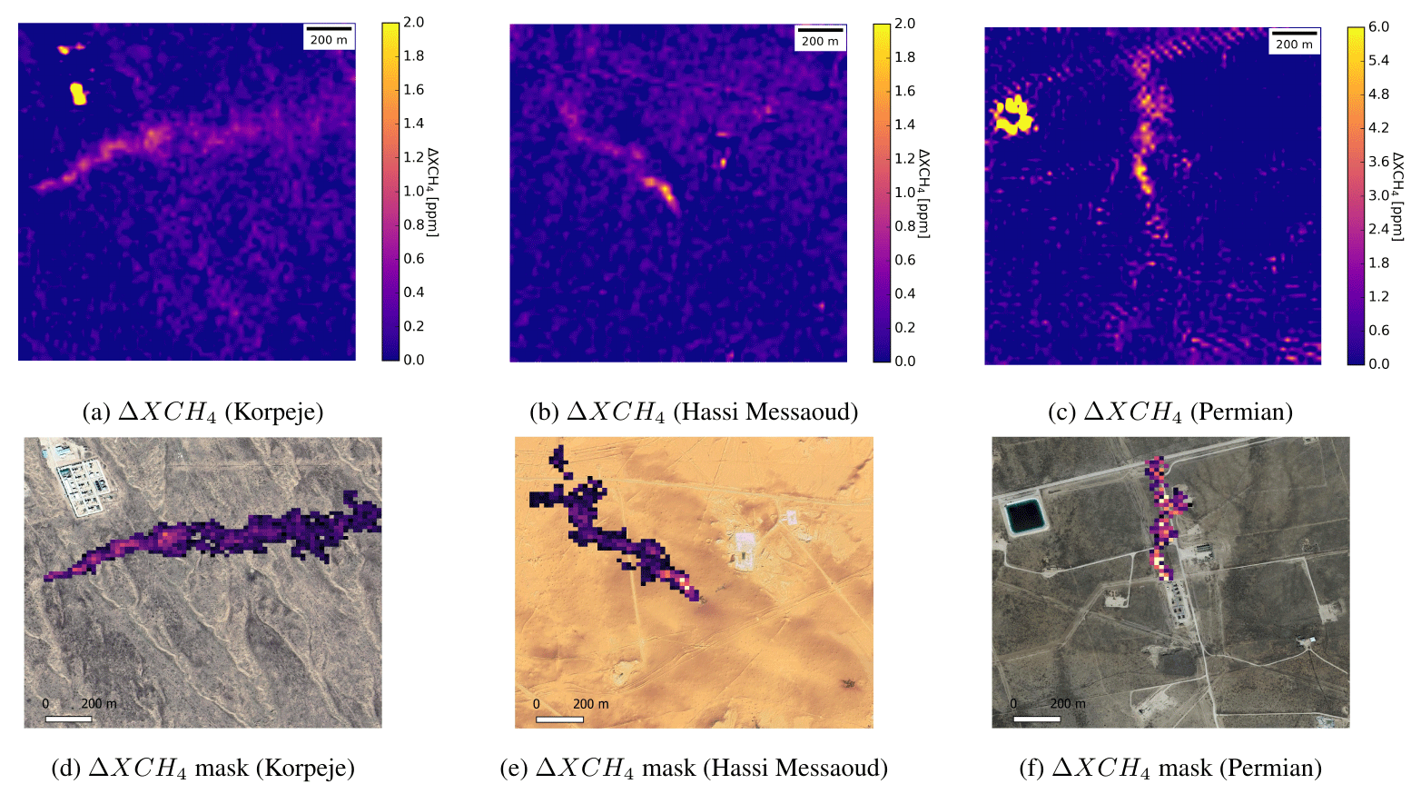
Figure 6 $\mathrm{\Delta }{X}_{{\mathrm{CH}}_{\mathrm{4}}}$ maps for the known methane point sources in Korpeje (a), Hassi Messaoud (b), and Permian Basin (c) O&G production regions. Panels (d), (e) and (f) background map from © Google Earth and © Microsoft Bing.

Figure 6 presents the $\mathrm{\Delta }{X}_{{\mathrm{CH}}_{\mathrm{4}}}$ map for each one of the three real emissions described here.

The maps show clear methane emissions at each one of the three sites combined with some outliers coming from different facilities and roads in the area. Figure 6f includes a granularity pattern that might be the result of inter-band and/or product registration. These enhancement maps have been converted into Q estimates as presented in Sect. 4. For the estimation of U_eff the average 10 m wind U₁₀ is required (Varon et al., 2021). We downloaded data from the NASA GEOS-FP meteorological reanalysis product at 0.25^∘ × 0.3125^∘ resolution (Molod et al., 2012) with values of 8.53174 m s⁻¹ for Korpeje, 5.589153 m s⁻¹ for Hassi Messaoud and 4.46345 m s⁻¹ for the Permian Basin. The flux rates Q estimated in each case were 12 091 ± 5220, 5453 ± 2200, and 19 698 ± 7585 kg h⁻¹, respectively.

Both the enhancement maps and the flux rates presented here indicate that the algorithm is capable of detecting methane and provide a quantification estimate within the expected range. However, this qualitative assessment cannot provide an accurate assessment of the algorithm's performance. The comparison against an accurate reference is recommended to understand the level of flux rate errors, the retrieved methane enhancement at a pixel level, and highlight potential algorithm improvements.

6 Simulation results

6.1 Retrieval results

The simulations for the three sites described in Sect. 3 were used to test the methane retrieval methodology described in Sect. 4.

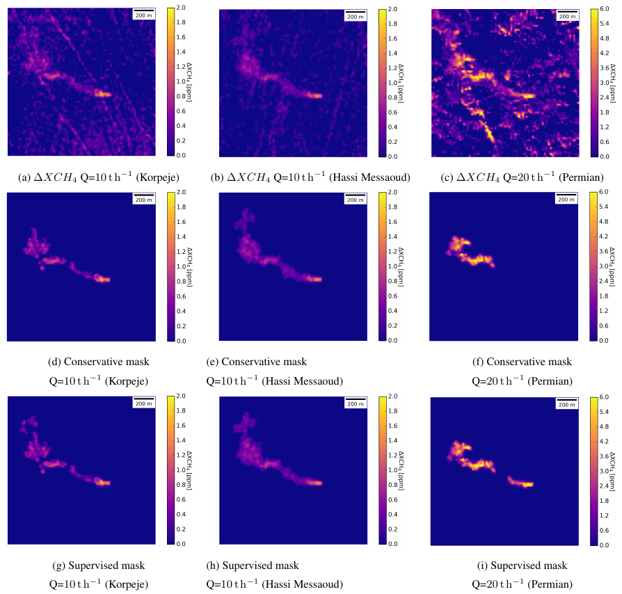
Figure 7 Results of the retrieval for the simulated datasets that include the map of $\mathrm{\Delta }{X}_{{\mathrm{CH}}_{\mathrm{4}}}$ values (a, b, c), the masked plumes obtained under a conservative masking criteria (d, e, f) and a supervised masking criteria (g, h, i). The selected simulations include the methane plume 2 (see Fig. 3b) with a flux rate Q=5000 kg h⁻¹ for Korpeje and Hassi Messaoud and Q = 20 000 kg h⁻¹ for the Permian Basin. Note the different color bar bounds for the Permian scene than for the Korpeje and Hassi Messaoud scenes.

Figure 7 illustrates an example of the map of $\mathrm{\Delta }{X}_{{\mathrm{CH}}_{\mathrm{4}}}$ values and the detection masked plumes (based on either a conservative or supervised criteria as defined in Sect. 4) against the validation reference obtained for a simulated dataset. This includes the methane plume 2 (see Fig. 3b) with a flux rate Q=5000 kg h⁻¹ for the Korpeje and Hassi Messaoud sites. A value of Q = 20 000 kg h⁻¹ was used for the map of $\mathrm{\Delta }{X}_{{\mathrm{CH}}_{\mathrm{4}}}$ values in the Permian Basin due to its higher surface heterogeneity.

For the Korpeje site, the methane plume with a flux rate Q = 10 000 kg h⁻¹ is clearly visible in the enhancement map in Fig. 7a. The major structure visible in the image is the dunes that follow a northwest to southeast direction. Similarly, Fig. 7b shows a visible plume in Hassi Messaoud over a similar dune structure but with slightly lower intensity. On the contrary, the enhancement map in the Permian Basin (Fig. 7c) presents a visible methane plume, but this is mixed with outliers despite its larger flux rate (Q = 20 000 kg h⁻¹).

The masking process shows positive results for the Korpeje and Hassi Messaoud sites (see Fig. 7d and g for Korpeje and Fig. 7e and h for Hassi Messaoud, respectively). Only the effect of the dune seems to have a small impact on the masking process with a slightly better detection for Hassi Messaoud with respect to Korpeje. The mask in Fig. 7d is smaller compared to Fig. 7g. By reducing the threshold of pixels required for detection changes between criteria (see Sect. 4) more pixels can be detected further along the plume. In the case of Hassi Messaoud, the average of two observations results in a smoother mask, and the plume shape is better defined.

When the process is repeated for the simulated plume over the Permian Basin, the masking process is still successful; however, it is highly affected by outliers in the surrounding area (e.g., oil rigs and roads in Fig. 2c). Figure 7f shows an example of this masking process where a significant area of the plume is detected. However, it does not include the pixels near the point source. By reducing the required number of pixels threshold to 20, those pixels near the source are detected (see Fig. 7i). Nevertheless, by setting this criteria several parts of the road crossing the entire image from north to south were also detected (see Fig. 2c). They were removed by masking the detected cluster that approximately defines the road.

The retrieval noise over the 300 × 1500 m² to the right of the plume (see Sect. 4) was for a conservative masking criteria of 251.7, 151.5 and 1488.2 ppb, respectively, for the Korpeje, Hassi Messaoud, and Permian Basin sites. These are the noise values that define the threshold in the masking process (see Sect. 4). The difference in the noise levels reported for each site closely correlates with the results presented in Fig. 7. When a supervised masking criteria is applied, the noise levels do not vary in the Korpeje and Permian Basin sites since the same normalization reference is used. However, the selection of the two closest S2 overpasses as a normalization for Hassi Messaoud reduces the noise down to 139.1 ppb.

The retrieval noise in the Korpeje and Hassi Messaoud sites is lower than the 21 %–49 % of an 1875 ppb methane background reported by Varon et al. (2021) (assuming an 1800 ppb background level, those noise levels correspond to 378–882 ppb). The lower value obtained here is likely the result of differences in retrieval methodology, location, scene size, outliers and temporal references. Nevertheless, the retrieval noise for the Permian Basin scene is much higher because that scene is much more heterogeneous.

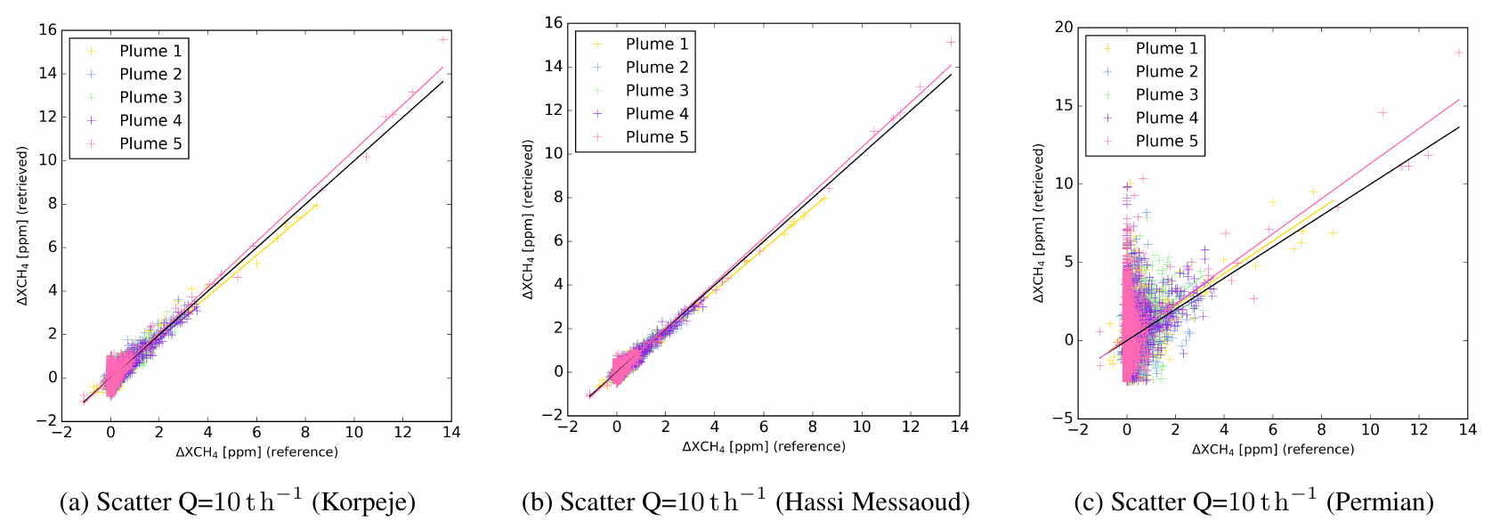
Figure 8 Scatter plots of the retrieval results against the validation reference at a pixel level for Korpeje (a), Hassi Messaoud (b) and the Permian Basin (c) for a simulation that includes the methane plume 2 (see Fig. 3b) scaled to a flux rate Q = 10 000 kg h⁻¹.

In addition to the retrieval maps and masked areas, Fig. 8 presents the scatter plot that compares the retrieved results against the methane enhancement reference at a pixel level:

Similarly to the ideal case shown in Fig. 5, the scatter plot of the retrieved $\mathrm{\Delta }{X}_{{\mathrm{CH}}_{\mathrm{4}}}$ values against the reference enhancement map presents a good agreement for Fig. 8a, b and c. The data points are more sparse in this case, as a consequence of the considerable noise levels of the S2 methane retrievals.

6.2 Flux rate validation

As was previously explained in Sect. 3, the methane plumes can be scaled at different flux rates and cover a wide range of possible emission levels. For both the Korpeje and Hassi Messaoud scenes, the Gorroño et al. (2021) datasets have been scaled to different flux rates from 0 to 20 000 kg h⁻¹. A step of 100 kg h⁻¹ is set from 600 to 3000 kg h⁻¹ so that the expected range of detection limits in the area can be accurately defined (Irakulis-Loitxate et al., 2022b). Larger steps of 500 and 1000 kg h⁻¹ define the rest of the covered range. For the Permian scene, the covered range goes from 0 to 50 000 kg h⁻¹. Due to the larger potential range of detection limits, a step of 200 kg h⁻¹ is set from 5000 to 15 000 kg h⁻¹. The step above 15 000 kg h⁻¹ is relaxed to 1000 kg h⁻¹.

For each one of the flux rates at each site, we obtained the Q value following the methodology in Sect. 4. Comparing the retrieved flux level against the simulation flux rate reference at each step defines a curve as a function of the flux rate that indicates the performance of the retrieval against our benchmark.

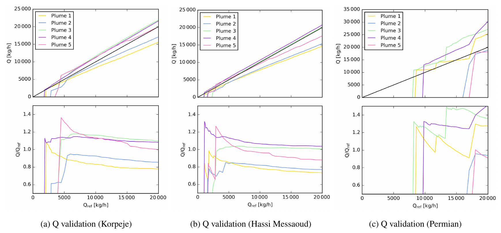
Figure 9 Q validation against reference values for a variety of plume shapes with a conservative detection masking criteria as detailed in Sect. 4.

Figure 9 shows the result of this procedure for the Korpeje, Hassi Messaoud and Permian Basin sites and the methane plume snapshots illustrated in Fig. 3. Here, a conservative detection masking criteria has been applied as detailed in Sect. 4.

The flux rate validation in Fig. 9a and b evidence a better than 20 % error in general. The bias is consistent across the different methane flux rates with a positive peak in some plumes near the detection limit. This effect is mainly visible in both plume 1 and plume 5 (see Fig. 3a and e), representing the most concentrated plumes.

Figure 9c presents the results for the Permian Basin. Due to its larger heterogeneity, the detection limit is considerably higher. Moreover, the curves present larger disagreement and a non-stable behavior. This can be explained by a large number of outliers in the image (see the blob-like shapes in Fig. 7c) that interfere with the plume mask.

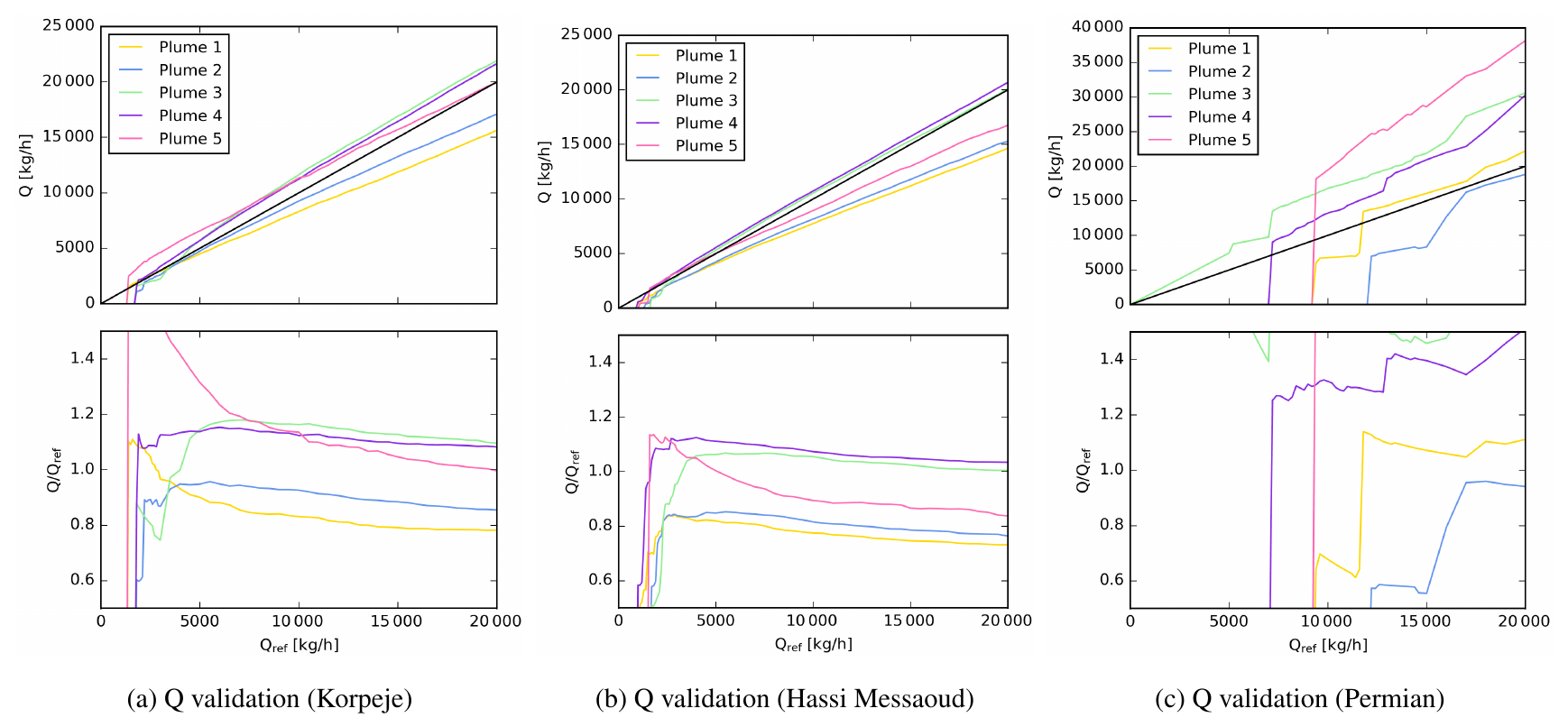
Figure 10 Q validation against reference values for a variety of plume shapes with a supervised detection masking criteria as detailed in Sect. 4.

Figure 10 shows the analogous results to Fig. 9 but with a supervised masking criteria as detailed in Sect. 4.

The results in Korpeje (see Fig. 10a) are highly similar to those in Fig. 9a. The lower threshold in the number of pixels also reduces the detection threshold leading to an increase in the peak levels in the relative error. Nonetheless, the opposite occurs in Hassi Messaoud (Fig. 10b), where the detection threshold is reduced together with the peaks close to it. In this case, the noise is lower (see Sect. 6.1) and suggests that these peaks are generated by the background noise below the masked area. Indeed, the comparison of the masked areas in the two cases showed that the lower noise was translated into a smoother background retrieval pattern and eventually into a better plume masking.

For the Permian site, the use of supervised masks significantly decreases the detection limit but at the expense of larger disagreements and non-stable trends (some of the trends are above the 50 % error limit). The first sampling of the flux rate jumps from 0 to 5000 kg h⁻¹. At this level, plume 3 can already be partially detected (the jump in the graph is the consequence of this sampling and not produced by an outlier detection). These results suggest that the significant disagreements are the consequence of an important effect of the background. For relatively small plume lengths, the underlying background is not only composed of noise but of a structure with blob-like features mixing with the methane signal. Thus, quantifying methane plumes becomes highly challenging for these heterogeneous and temporally variant sites, and specific management of these background features might be needed.

Interestingly, this validation is also helpful to provide an estimation of the detection limit for each site and plume. From Figs. 9 and 10 we can identify the first flux values at which the plume can be captured.

Table 1 Methane flux rate detection limit for the selected sites at Korpeje (Turkmenistan) (see Fig. 2a), Hassi Messaoud (Algeria) (see Fig. 2b) and the Permian Basin (USA) (see Fig. 2c) under two different detection masking criteria (conservative and supervised) detailed in Section 4.

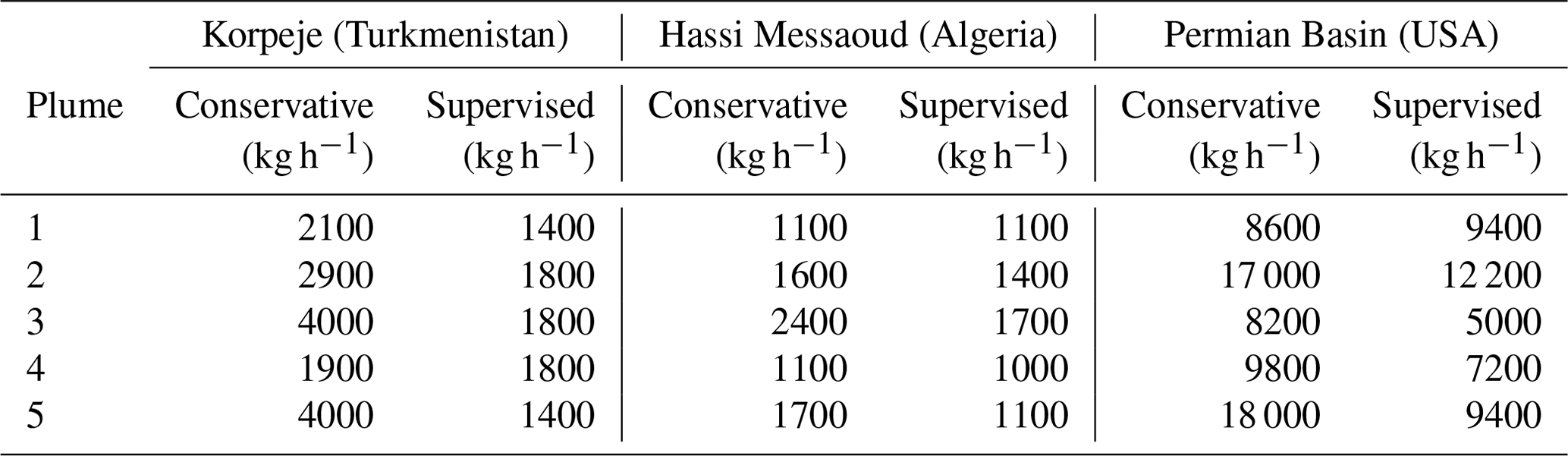
Table 1 includes the detection limit for the masking criteria proposed and the three sites considered in Sect. 2.

The validation for Korpeje in Fig. 9a shows a detection limit that ranges from 1900 to 4000 kg h⁻¹ with a conservative masking criteria. They are significantly reduced to levels from 1400 to 1800 kg h⁻¹ using supervised masking. Similarly, the results in Hassi Messaoud span from 1100 to 2400 kg h⁻¹ with a conservative masking criteria and from 1100 to 1700 kg h⁻¹ under supervised masking criteria.

These results are coherent with the thresholds reported by Varon et al. (2021) (2600 kg h⁻¹ for an approximately 500 ppm retrieval noise). In the specific case of Korpeje, the reported value of 1800 kg h⁻¹ in Irakulis-Loitxate et al. (2022b) is in the same ranges as those presented in Table 1. For the Permian Basin, the results suggest that the detection limit varies highly depending on the plume shape (in combination with the underlying structure). The values are typically in the order of 10 000 kg h⁻¹ down to 5000 kg h⁻¹ under the best conditions.

6.3 Extending the validation to a large plume dataset and season changes

Section 6.2 has shown a detailed validation for five plumes at three different O&G facilities. This subsection intends to complement the previous analysis by expanding the number of methane plume snapshots and considering a different time of year. The former is extended by considering 221 plume snapshots and are obtained from the same LES simulation as in Fig. 3 sampled every 2.5 min within plumes 1 and 5. The latter includes observations around the winter solstice in contrast to the ones studied in Sect. 6.2, which correspond to observations close to the summer solstice in the Northern Hemisphere. This selection should reflect maximum changes in the solar angle in addition to phenological and atmospheric changes.

In order to reduce the amount of processed data, the methane flux rate is only scaled to six different values. Those are 500, 1000, 1500, 2000, 2500 and 3000 kg h⁻¹ for Korpeje and Hassi Messaoud and 1500, 2500, 5000, 7500, 10 000 and 12 500 kg h⁻¹ for the Permian Basin. Rather than producing a validation curve, this exercise will generate an error distribution at each one of the flux rate levels. Instead of an specific detection limit, the result will be a percentage of plumes detected for each flux rate level.

Figure 11 Q validation against reference values for 221 plume shapes with supervised detection masking criteria as detailed in Sect. 4. The graph also includes the mean and standard deviation of the errors at the selected flux rate levels.

Table 2 Statistics associated to Fig. 11. This includes the percentage of plumes detected, the mean error and standard deviation against simulated benchmarks for the selected sites at Korpeje (Turkmenistan) (see Fig. 2a), Hassi Messaoud (Algeria) (see Fig. 2b) and the Permian Basin (USA) (see Fig. 2c) under the supervised masking criteria detailed in Sect. 4.

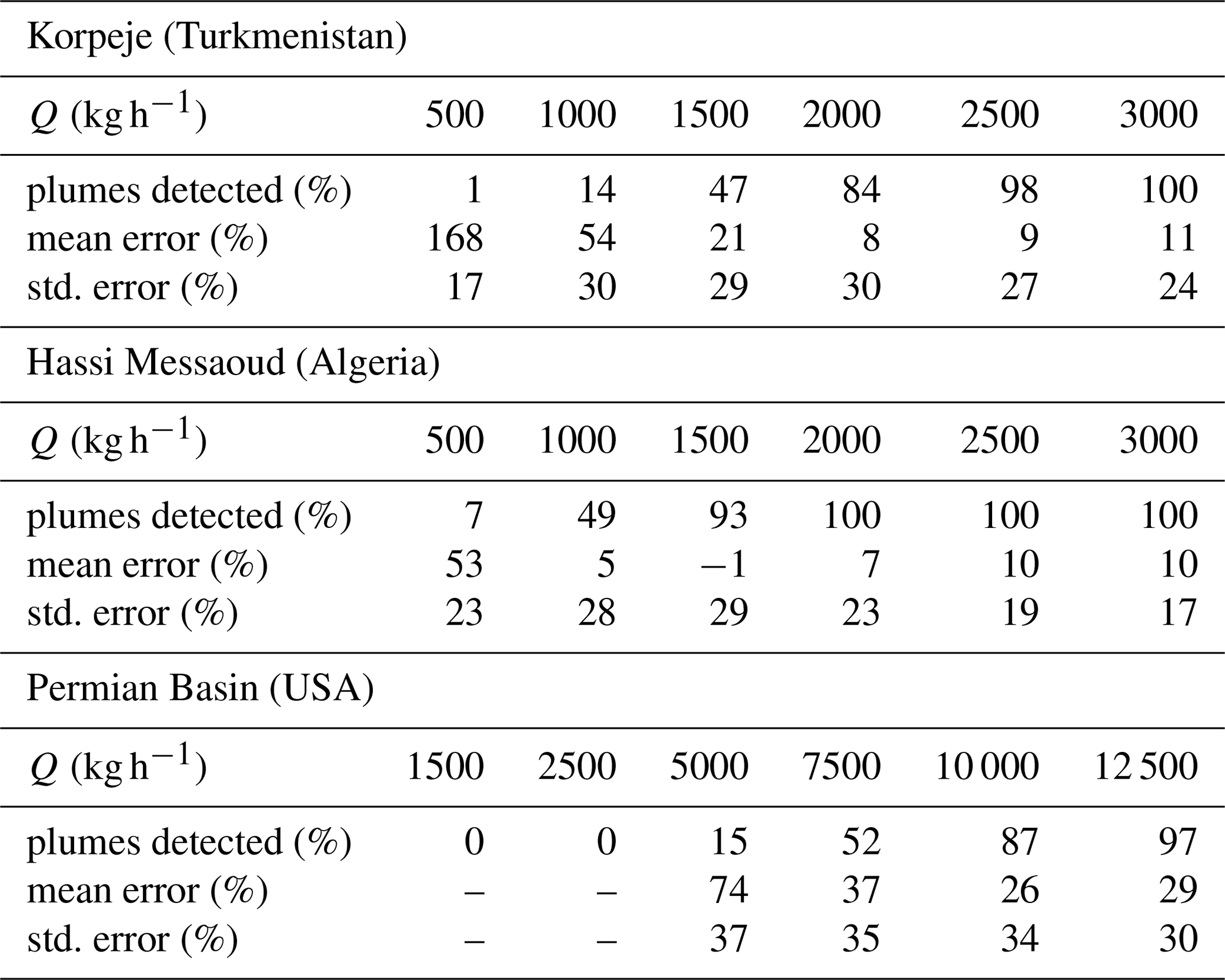
Figure 11 includes the results at the specified flux rate levels. It includes the error for each of the 221 snapshots as well as the mean and standard deviation error at each one of the specified flux rates. Table 2 summarizes these mean and standard deviation metrics in addition to the percentage of methane plumes detected. The products and sites are equivalent to those in Sect. 6.2. A supervised detection masking criteria as detailed in Sect. 4 has been selected for this exercise.

In terms of detection limit, these results support the previous estimates. Around half of the methane plumes are detected at Korpeje over 1500 kg h⁻¹. This is reduced to just 1000 kg h⁻¹ in Hassi Messaoud and scaled up to 7500 kg h⁻¹ in the Permian Basin. The mean error fluctuates when the percentage of plumes detected is small. At these flux rates, the algorithm tends to detect those plumes with a more concentrated emission and does not fully represent a general trend. For a flux rate of 3000 kg h⁻¹ in Korpeje and Hassi Messaoud, the mean error is around 10 %, whereas this is up to 30 % for a flux rate of 12 500 kg h⁻¹ in the Permian Basin. The latter was discussed in Sect. 6.2 and can be attributed to the large noise patterns in the methane enhancement retrieved. The small general overestimation at Korpeje and Hassi Messaoud slowly declines with larger flux rates, as illustrated in Fig. 10. The dispersion of the results is reduced in relative terms with increasing flux rates with values ranging in the 20 to 30 % in Korpeje and Hassi Messaoud and 30 % to 40 % in the Permian Basin.

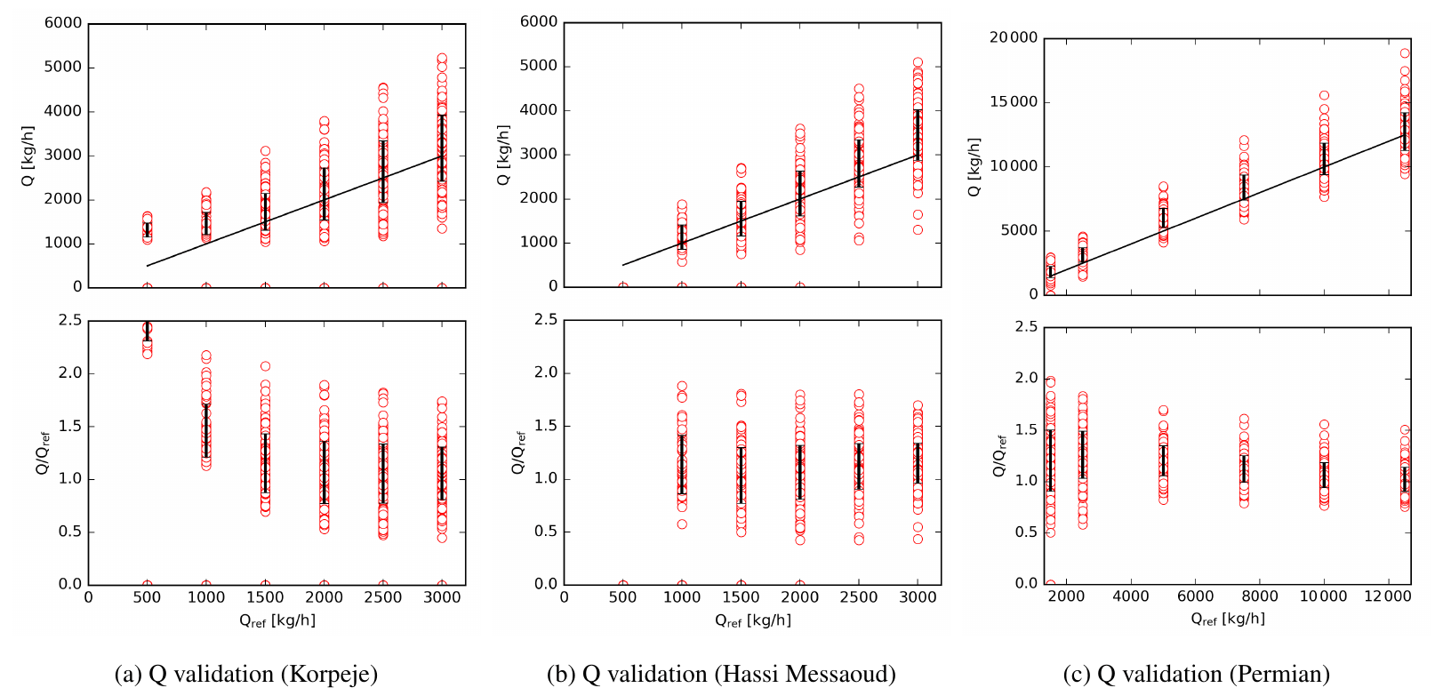
Figure 12 Q validation against reference values for acquisitions near the winter solstice. Similarly to Fig. 11, the validation is set for 221 plume shapes with a supervised detection masking criteria as detailed in Sect. 4. The graph also includes the mean and standard deviation of the errors at the selected flux rate levels.

Table 3 Methane flux rate detection limit for the selected sites at Korpeje (Turkmenistan) (see Fig. 2a), Hassi Messaoud (Algeria) (see Fig. 2b) and the Permian Basin (USA) (see Fig. 2c) under the two different detection masking criteria (conservative and supervised) detailed in Sect. 4.

The selected dates in the previous examples are close to the summer solstice in the Northern Hemisphere. Figure 12 and Table 3 summarize analogous results to those in Fig. 11 and Table 2 but for acquisitions close to the winter solstice. The selected overpasses were S2A on the 9 January 2021, S2A on 13 January 2021 and 16 December 2020 for Korpeje, Hassi Messaoud and the Permian Basin, respectively. For the temporal normalization, we selected the S2A acquisitions on 20 December 2020 and 19 January 2021 for Korpeje, the S2B acquisitions on 8 and 18 January 2021 for Hassi Messaoud and the S2A acquisitions on 6 and 26 December 2020 for the Permian Basin.

The detection limit increases slightly for Hassi Messaoud (around half of the plumes are detected from 1000 to 1500 kg h⁻¹ as compared to 1000 kg h⁻¹ in the summer case). The result is expected since the higher sun zenith angle reduces the reflected radiance and increases the anisotropic effects of the surface. This situation does not occur in Korpeje with very similar results, if not better, in the winter solstice. Temporal normalization in Hassi Messaoud is analogous both in winter and summer conditions with a mean of the two closest S2B acquisitions. On the contrary, the temporal normalization for Korpeje differs with just one S2B observation for the summer case and the mean of the closest S2A acquisitions in the winter case.

The results for the Permian Basin show very large differences between the summer and winter cases. The temporal normalization in this case selected the two closest S2A acquisitions, whereas only one S2B acquisition was selected during the summer due to cloud conditions and large temporal variations. Indeed, the temporal variations due to phenology changes and atmospheric conditions, determine the detection capabilities to a large extent in this site. The scene classification of the S2 L2A products indicated no vegetation for almost all the pixels in the selected area, while the summer case presented a mixture of vegetated and non-vegetated ones. The winter scenario registers a higher sun zenith angle, but the vegetation largely disappears. Combined with cloud-free conditions as in the example, the detection limit can improve significantly.

6.4 Understanding the flux rate uncertainty sources

The results in Figs. 9 and 10 show generally good agreement between retrieved and benchmarked emission rates. The disagreement can arise from either the retrieval of the $\mathrm{\Delta }{X}_{{\mathrm{CH}}_{\mathrm{4}}}$ map, its masking process or the IME to Q conversion. The first of these might be generated by the limited accuracy of the LUT (see Sect. 6.1) or the underlying structure and noise below the masked area (see Sect. 6.2).

The validation results in Korpeje and Hassi Messaoud (see Fig. 10a and b) show that the error for each individual plume lies approximately between ±20 % of the reference flux rate. This is confirmed by the results in Sect. 6.3, which resulted in typical dispersion levels of 20 %–30 % (see Tables 2 and 3). This is a correlated error among the different methane flux rate levels but is apparently uncorrelated among each individual plume. In this case, neither the $\mathrm{\Delta }{X}_{{\mathrm{CH}}_{\mathrm{4}}}$ retrieval map nor the underlying background features are expected to constitute a major source of error. Thus, these systematic errors are expected to arise from the U_eff associated with the IME-to-Q conversion.

Here, all the snapshots in the WRF-LES simulation were considered, and a specific U_eff was generated based on the dataset considered for the simulations (see Sect. 3). Each plume has been scaled to 10 000 kg h⁻¹, and the relationship between the U_eff and U₁₀ was established with a Huber regressor (Huber and Ronchetti, 2011). Figure 13 reports the specific U_eff regression curve and compares it to the U_eff calibration reported in Varon et al. (2021).

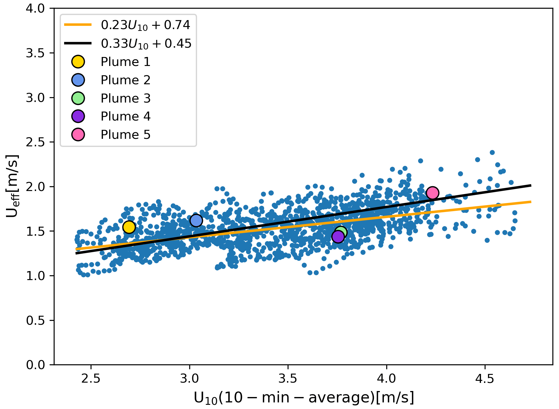
Figure 13 U_eff calibration for the specific simulation dataset (see Sect. 3) at a flux rate of 10 000 kg h⁻¹. The yellow line fits a Huber regressor to the data. The black line shows the U_eff fit of Varon et al. (2021) based on a set of 25 m LES.

The results indicate that the uncertainty on the U_eff calibration depends not only on that of U₁₀ but also on the fitting knowledge. This fitting knowledge can be further separated into a systematic component and a random one. The former depends on the WRF-LES simulation and its specific parameterization: emission altitude, surface roughness, turbulence, …. These simulation datasets and the retrieval methodology will generate different relationships between the U_eff and U₁₀. This error is relatively small for this specific example (0 %–9 % error for the five plumes considered) with higher disagreement the higher U₁₀ is for a linear fitting. However, it is a critical source of uncertainty for the assessment of emissions over O&G areas since these errors will largely remain correlated under similar atmospheric conditions and, consequently, largely remain in the uncertainty budget for the area studied.

The latter effect is the consequence of differences in the U_eff value between snapshots, and it results in an uncorrelated error between methane plume snapshots. The root mean squared error between the U_eff calibration and the individual snapshots in Fig. 13 is 0.20. This represents a substantial error in relative terms that ranges from 10 % to 20 %. This uncertainty source generally dominates for a single plume emission estimation, especially at lower U₁₀ values. However, its uncorrelated nature with other methane plume emissions means its impact will decrease when an O&G area of several point-source emissions is studied. Large levels of turbulence will impact on the dispersion of the U_eff calibration values due to larger dispersion of the $\mathrm{\Delta }{X}_{{\mathrm{CH}}_{\mathrm{4}}}$ snapshots and the averaged U₁₀ values. This error would ideally be zero if the dissipation of the plume occurred by uniform transport downwind of the source. The oscillation error between each plume in Figs. 9 and 10 is inversely correlated to the specific plume deviations in Fig. 13.

Thus, the major sources of uncertainty for the reported flux rates are the U₁₀ uncertainty (∼ 50 % when using a meteorological reanalysis product (Varon et al., 2018)), a systematic uncertainty of U_eff in the range 0 %–9 % and a random fitting uncertainty between 10 % and 20 %, a $\mathrm{\Delta }{X}_{{\mathrm{CH}}_{\mathrm{4}}}$ retrieval accuracy (typically below 10 %) and the impact of background features under the detection mask mainly applicable to heterogeneous and temporally variant scenes.

7 Conclusions and further work

This work presents a methodology and implementation to generate Sentinel-2 benchmark products with simulated methane plumes. The method keeps the original S2 observations and adds the simulated methane plume transmittance over the reflectance map. It also includes a compensation term in the calculated total atmospheric transmittance capable of correcting, with a negligible residual, for the bias introduced by convolving a signal that corresponds to an already band-integrated quantity.

The proposed algorithm for the generation of a Sentinel-2 $\mathrm{\Delta }{X}_{{\mathrm{CH}}_{\mathrm{4}}}$ map retrieves methane concentration enhancements from an estimated methane transmittance image. This methane transmittance is calculated as the ratio between the reflectance at a spectral channel affected by methane absorption and a methane-free reference band. This algorithm has been validated against the Sentinel-2 benchmark products in a real context, where it was also possible to define a minimum emission detection threshold for specific sites and methane plumes. The scaling of these products and a comparison against reference source magnitudes results in the validation of the retrieval at different flux rate levels and conditions. We find that for homogeneous and temporally invariant surface types, a detection limit of 1000 to 2000 kg h⁻¹ is feasible for S2. For these types of surface, the validation resulted in an excellent agreement (within ±20 %) largely depending on the plume shape. For areas with a large surface heterogeneity and temporally variant, the detection limit rises considerably over 5000 kg h⁻¹. In these cases, the masking process becomes very sensitive to small variations due to the surface structure underlying the methane point sources. That results in a larger spread of disagreements depending on the plume shape and masked area.

The study was also capable of separating the different uncertainty sources associated to the flux rate estimates. The effective wind speed (U_eff) calibration has been tuned with the specific LES simulation and, in addition to the uncertainty associated to the 10 m wind speed (U₁₀), it describes both a systematic and a random fitting error. The former effect largely depends on the WRF-LES simulation dataset and fitting method. The disagreement between fitting curves here was relatively small for this specific example (0 %–9 % error for the five plumes considered) with higher disagreement the higher U₁₀ is. The latter effect represents the departures from the U_eff calibration between snapshots, for which we found a root mean squared error of 0.20, representing a substantial error in relative terms that ranges from 10 % to 20 %. However, when considering its effect over multiple plumes across an O&G area its impact will largely decrease due to the uncorrelated nature of the error between individual methane plume snapshots. In contrast, the systematic component might be highly correlated under similar atmospheric conditions and, consequently, largely remain in the uncertainty budget for the studied O&G area. Finally, the study of heterogeneous and temporally variant scenes indicates the large impact of background features under the detection mask. In these cases, it is possible that this uncertainty contribution becomes relevant, or even dominates the uncertainty budget.

The study presented here can be rapidly applied to any other mission, including Landsat, CHIME, or EnMAP. For each specific mission, a set of simplifications might reduce the computational costs, such as the assumption of a spectrally constant surface reflectance ρ_surface. For example, this simplification could significantly reduce the computational time with a minor error on the benchmark products.

Further evolutions of the methodology might seek to refine the link between the modeled WRF-LES plumes and the reference $\mathrm{\Delta }{X}_{{\mathrm{CH}}_{\mathrm{4}}}$ map. Among different improvements we can include the consideration of the scene altitude to provide a better estimation of the column of dry air Ω_a (see Eq. 1), the selection of WRF-LES plumes with finer spatial resolution or the possibility to consider the point spread function of the instrument to generate a more realistic total transmittance map.

The accuracy of the retrieved $\mathrm{\Delta }{X}_{{\mathrm{CH}}_{\mathrm{4}}}$ map largely depends on the selected observations for acquisition and normalization. Figure 1 highlights the better positioning of S2A B12 with respect to S2B B12 for methane detection. The examples selected here considered detections using S2A satellite unit. Preliminary tests over Hassi Messaoud indicate a small difference between S2A and S2B. However, it requires a large dataset study to precisely evaluate those differences. For the temporal normalization, we have seen how the noise was reduced from 151.5 ppb down to 139.1 ppb in Hassi Messaoud when the temporal normalization selects the two closest S2 overpasses. The results for the Permian Basin evidence how understanding the phenology of the site might determine large variation in detection thresholds based on rapid temporal changes and surface heterogeneity. General guidelines for temporal normalization can be extracted at this point, such as the selection of the closest acquisitions if the site rapidly changes or the selection of the same viewing configuration if the site presents a strong surface directionality. However, temporal normalization must be assessed on a case-by-case basis where possible since it requires a complex understanding of different effects that involve the consideration of different orbit viewing overpasses, satellite spectral and geometric differences, as well as the site temporal variation itself.

The development of these simulations is expected to be helpful in testing novel approaches for upcoming temporal normalization methodologies, such as in Ehret et al. (2022). Furthermore, the generation of realistic and accurate simulated datasets might be helpful to train upcoming machine learning methodologies, such as the one presented in Jongaramrungruang et al. (2022).

The use of complementary methodologies and the continuous validation of the methane emissions is key for the generation of robust estimates that contribute to the development of a global and systematic monitoring of methane emission from the O&G sector. For example, the results presented here are consistent with those reported by Sherwin et al. (2022) based on an in situ campaign in Arizona where controlled methane releases validated several missions and retrieval algorithms.