Derivation of depolarization ratios of aerosol fluorescence and water vapor Raman backscatters from lidar measurements

Polarization properties of the fluorescence induced by polarized laser radiation are widely considered in laboratory studies. In lidar observations, however, only the total backscattered power of fluorescence is analyzed. In this paper we present results obtained with a modified Mie–Raman–fluorescence lidar operated at the ATOLL observatory, Laboratoire d'Optique Atmosphérique, University of Lille, France, allowing us to measure depolarization ratios of fluorescence at 466 nm (δ_F) and of water vapor Raman backscatter. Measurements were performed in May–June 2023 during the Alberta forest fires season when smoke plumes were almost continuously transported over the Atlantic Ocean towards Europe. During the same period, smoke plumes from the same sources were also detected and analyzed in Moscow, at the General Physics Institute (GPI), with a five-channel fluorescence lidar able to measure fluorescence backscattering at 438, 472, 513, 560 and 614 nm. Results demonstrate that, inside the planetary boundary layer (PBL), the urban aerosol fluorescence is maximal at 438 nm, and then it gradually decreases with the increase in wavelength. The smoke layers observed within 4–6 km height present a maximum fluorescence at 513 nm, while in the upper troposphere, fluorescence maximum shifts to 560 nm. Regarding the fluorescence depolarization ratio, for smoke its value typically varies within the 45 %–55 % range.

The depolarization ratio of the water vapor Raman backscattering at 408 nm is shown to be quite low (2±0.5 %) in the absence of fluorescence because the narrowband interference filter (0.3 nm) in the water vapor channel selects only the strongest vibrational lines of the Raman spectrum. As a result, the depolarization ratio at the water vapor Raman channel is sensitive to the presence of strongly depolarized fluorescence backscattering and can be used for the evaluation of the aerosol fluorescence contribution to measured water vapor mixing ratio.

1 Introduction

The possibility to measure the laser-induced fluorescence becomes an important added value to existing Mie–Raman lidars because fluorescence measurements provide new independent information about aerosol properties. Nowadays, the spectroscopic lidars based on 32-channel PMT combined with spectrograph proved the ability to measure the fluorescence spectrum (Sugimoto et al., 2012; Reichardt, 2014; Reichardt et al., 2018, 2023; Richardson et al., 2019; Liu et al., 2022). On the other hand, lidars, with a single fluorescence channel, can be widespread due to their simplicity (Rao et al., 2018; Veselovskii et al., 2020). Such single-channel fluorescence lidars, combined with depolarization measurements at the elastic wavelength, provide new independent information about aerosol type (Veselovskii et al., 2022). However, in all lidar studies, only the total scattered power was analyzed, while the polarization properties of the fluorescence were ignored. At the same time, fluorescence depolarization measurements are widely used in laboratory research (Lakowicz, 2006). When polarized laser radiation is used for excitation, the fluorescence emission is also partly polarized and the degree of its depolarization (anisotropy) depends on the fluorescence lifetime, on the angle between excitation and emission dipoles, and on the rotational mobility of molecules (Lakowicz, 2006). In the fluorescence spectroscopy, the polarization state of emission is described by the anisotropy (Lakowicz, 2006), introduced as

$$\begin{array}{}\text{(1)}& r={\displaystyle \frac{P_{\mathrm{F}}^{\parallel }-P_{\mathrm{F}}^{\perp }}{P_{\mathrm{F}}^{\parallel }+\mathrm{2}{P}_{\mathrm{F}}^{\perp }}},\end{array}$$

where $P_{\mathrm{F}}^{\parallel }$ and $P_{\mathrm{F}}^{\perp }$ are the powers of co- and cross-polarized fluorescence components. In lidar measurements, however, the fluorescence depolarization ratio, δ_F, is given as

$$\begin{array}{}\text{(2)}& {\mathit{\delta }}_{\mathrm{F}}={\displaystyle \frac{P_{\mathrm{F}}^{\perp }}{P_{\mathrm{F}}^{\parallel }}}.\end{array}$$

Therefore, the anisotropy is expressed as a function of the δ_F as follows:

$$\begin{array}{}\text{(3)}& r={\displaystyle \frac{\mathrm{1}-{\mathit{\delta }}_{\mathrm{F}}}{\mathrm{1}+\mathrm{2}{\mathit{\delta }}_{\mathrm{F}}}}.\end{array}$$

For randomly oriented fluorophores with collinear absorption and emission dipoles, in the absence of rotational motion, the anisotropy r=0.4 (Lakowicz, 2006), which corresponds to δ_F= 33 %. This is the minimal value one can expect in lidar measurements. The existence of any angle between absorption and emission dipoles, as well as molecule rotation in the process of emission, will increase δ_F (Lakowicz, 2006). Thus, measurement of fluorescence depolarization ratio may bring additional information about atmospheric aerosol, as we will show below.

Water vapor is a key atmospheric component playing an essential role in the planet's radiative balance, and Raman lidars today are widely used for such observations (Whiteman, 2003; Chouza et al., 2022, and references therein). However, when the UV laser beam passes through a smoke layer, the broadband fluorescence signal is induced and its spectrum includes the region of water vapor Raman lines. Thus, the signal in the water vapor channel (around 407.5 nm, when 354.7 nm laser radiation is emitted) becomes contaminated by the fluorescence backscatter signal (Immler et al., 2005; Immler and Schrems, 2005). This contamination can be reduced by decreasing the width of the transmission band in the water vapor channel down to 10ths of nanometers. However, as was shown recently, fluorescence still remains the source of uncertainties, especially when the water vapor mixing ratio (WVMR) is measured inside the smoke layers in the upper troposphere (Chouza et al., 2022; Reichardt et al., 2023).

Depolarization measurements provide an opportunity to monitor the presence of fluorescence signals in the Raman channel. The Q branch of water vapor Raman lines (near 407.5 nm) provides a weakly depolarized backscatter, while fluorescence is strongly depolarized. Thus, the presence of fluorescence should increase the depolarization ratio of the signal in the water vapor channel. Moreover, if the depolarization ratios of water vapor and fluorescence are known, the contribution of fluorescence to the measured WVMR can be evaluated.

In this article, we report and analyze, for the first time, the depolarization ratio of aerosol fluorescence and of water vapor Raman backscatter from lidar observations performed at the ATOLL observatory (ATmospheric Observation at liLLe), Laboratoire d'Optique Atmosphérique, University of Lille, during dense smoke events occurring in May–June 2023. We start with a description of the experimental setup in Sect. 2.1 and derive, in Sect. 2.2, the main equations for estimating the fluorescence contribution to the water vapor Raman channel. In the first part of the results section (Sect. 3.1), the fluorescence depolarization ratios over ATOLL are analyzed for different aerosol types. The measurements of fluorescence spectra performed with a new five-channel fluorescence lidar, operated in Moscow, are presented in Sect. 3.2. In Sect. 3.3, we analyze the depolarization ratio in the water vapor Raman channel and estimate the contamination of fluorescence in the derived WVMR profiles. Finally, in Sect. 4 we present our conclusions.

2 Experimental setup and data analysis

2.1 Lidar system

In our study, two lidar systems are considered. The first one, LILAS (LIlle Lidar AtmosphereS), is a multiwavelength Mie–Raman–fluorescence lidar, whereas the second one is a multiwavelength fluorescence lidar operated by the General Physics Institute (GPI), Moscow (Veselovskii et al., 2023). Both systems are based on a tripled Nd:YAG laser (Q-smart 450) with a 20 Hz repetition rate and pulse energy about of 100 mJ at 355 nm. The backscattered laser light in both systems is collected by a 40 cm aperture telescope, and the lidar signals are digitized with transient recorders (Licel) with 7.5 m range resolution, allowing simultaneous detection in the analog and photon counting modes.

LILAS allows the so-called $\mathrm{3}\mathit{\beta }+\mathrm{2}\mathit{\alpha }+\mathrm{3}\mathit{\delta }$ configuration, including three particle backscattering (β₃₅₅, β₅₃₂, β₁₀₆₄), two extinction (α₃₅₅, α₅₃₂) coefficients, and three particle depolarization ratios (δ₃₅₅, δ₅₃₂, δ₁₀₆₄). The Raman channel with a $\mathrm{407.54}/\mathrm{0.3}$ nm spectral width interference filter allows also water vapor profiling. At the end of 2019, the lidar was modified to enable fluorescence measurements. A part of the fluorescence spectrum is selected by a wideband interference filter of 44 nm width centered at 466 nm (Veselovskii et al., 2020).

In the fluorescence lidar of GPI only a 355 nm wavelength is emitted, while fluorescence is measured in five spectral intervals. The central wavelengths and widths of spectral transmission bands (in parentheses) are 438 (29), 472 (32), 513 (29), 560 (40) and 614 (54) nm (Veselovskii et al., 2023). Thus, the fluorescence spectrum could be sampled at five different wavelengths. The transmission bands of the fluorescence channels (Fig. 1 in Veselovskii et al., 2023) are separated, and there are no cross-talks between the channels. At GPI, the measurements were performed at an angle of 48 ^∘ to the horizon. The strong sunlight background restricts the fluorescence observations of both systems to only the nighttime hours.

Several aerosol properties can be derived from fluorescence. The fluorescence backscattering coefficient, β_Fλ, at wavelength λ_F, is calculated from the ratio of fluorescence and nitrogen Raman backscattering signals, as described in Veselovskii et al. (2020). Remember that β_Fλ is related to fluorescence signals integrated over the filter transmission band D_λ. In Moscow measurements are performed at five wavelengths, and to compare β_Fλ between different channels one makes use of the “fluorescence spectral backscattering coefficient” $B_{\mathit{\lambda }}=\frac{{\mathit{\beta }}_{\mathrm{F}\mathit{\lambda }}}{D_{\mathit{\lambda }}}$ (fluorescence backscattering per spectral interval). LILAS has only one single fluorescence channel; therefore, when presenting data from LILAS, for the sake of simplicity, one uses the notation β_F466=β_F. The intensive property characterizing aerosol fluorescence is the fluorescence capacity G_Fλ, which is the ratio of the fluorescence backscattering at wavelength λ_F to the backscattering coefficient at laser wavelength $G_{\mathrm{F}\mathit{\lambda }}=\frac{{\mathit{\beta }}_{\mathrm{F}}}{{\mathit{\beta }}_{\mathit{\lambda }}}$. This ratio, in principle, can be calculated for any laser wavelength. For LILAS observations G_Fλ is calculated with respect to β₅₃₂, as β₅₃₂ is derived with rotational Raman scattering and it does not depend on assumption about the Ångström exponent (Veselovskii et al., 2015). Again, when presenting LILAS data, for simplicity one will use the notation G_Fλ=G_F. In this work, all profiles of aerosol properties are smoothed with the Savitzky–Golay method, using second-order polynomials with eight points in the spatial window.

Additional information about the atmospheric thermodynamic state was available from radiosonde measurements performed at Herstmonceux (UK) and Beauvechain (Belgium) stations, located 160 and 80 km away from the ATOLL observatory, respectively. When calculating the relative humidity, the water vapor profiles measured by Raman lidar and temperature profiles provided by the radiosonde were used.

As discussed in Sect. 1, measurements of the fluorescence depolarization ratio and the depolarization of water vapor Raman backscatter are expected to bring new information about aerosol properties and fluorescence contamination in the water vapor Raman channel. In 2023, LILAS was upgraded to allow depolarization measurements at both 466 and 408 nm. The corresponding optical layout is shown in Fig. 1. Dichroic mirrors (DMs) separate the 387, 408 and 466 nm components, while polarizing cubes split the components with polarizations oriented parallel and perpendicular to the emitted polarized laser beam. For both channels, the polarizing cube PBS251 from Thorlabs was used. The fluorescence depolarization ratio, δ_F, and the water vapor Raman scattering depolarization ratio, δw, are both defined and calculated as a ratio of the perpendicular to the respective parallel components. The calibration of both ratios was performed as described in Freudenthaler et al. (2009). The uncertainty of calibration is estimated to be below 15 % for both 466 and 408 nm channels.

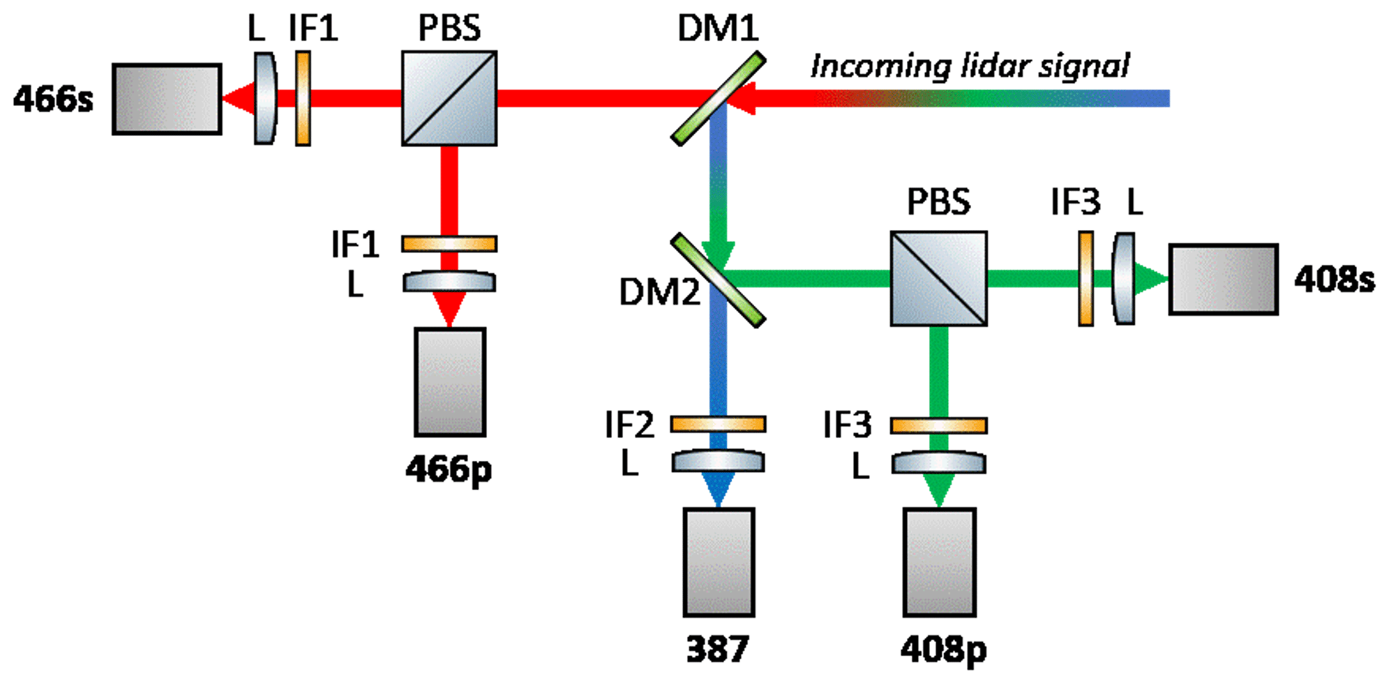
Figure 1 Optical layout of depolarization measurements at 408 nm and 466 nm wavelengths. L – lens; IF1–IF3 – interference filters; DM1 and DM2 – dichroic mirrors; PBS – polarizing cube.

2.2 Expressions for estimating fluorescence impact on water vapor measurements

As discussed in the recent work of Chouza et al. (2022) and Reichardt et al. (2023), the broadband aerosol fluorescence is expected to contribute to the signal measured at the water vapor Raman channel. Below, we provide the basic equations for estimating this contribution, based on the measurements of the depolarization ratio in the water vapor Raman channel. The elastic backscattered radiative power, at the laser wavelength λ_L from distance z, can be modeled, after background subtraction, by writing the following lidar equation:

$$\begin{array}{}\text{(4)}& P_{\mathrm{L}}=O\left(z\right){\displaystyle \frac{\mathrm{1}}{z^{\mathrm{2}}}}{C}_{\mathrm{L}}\mathit{\beta }{T}_{\mathrm{L}}^{\mathrm{2}},\end{array}$$

where O(z) is the geometrical overlap factor, which is assumed to be the same for all channels. C_L is a range-independent constant, including efficiency of the detection channel, the emitted laser power and the receiving telescope diameter. T_L is the one-way atmospheric transmission, describing light losses on the way from the lidar to distance z at wavelength λ_L.

$$\begin{array}{}\text{(5)}& T_{\mathrm{L}}=\exp \left\{-\underset{\mathrm{0}}{\overset{z}{\int }}\left[{\mathit{\alpha }}^{\mathrm{a}}({\mathit{\lambda }}_{\mathrm{L}},z^{\prime })+{\mathit{\alpha }}^{\mathrm{m}}({\mathit{\lambda }}_{\mathrm{L}},z^{\prime })\right]\mathrm{d}{z}^{\prime }\right\}\end{array}$$

The backscattering and extinction coefficients contain the aerosol (a) and molecular (m) contributions: ${\mathit{\beta }}_{{\mathit{\lambda }}_{\mathrm{L}}}={\mathit{\beta }}_{{\mathit{\lambda }}_{\mathrm{L}}}^{\mathrm{a}}+{\mathit{\beta }}_{{\mathit{\lambda }}_{\mathrm{L}}}^{\mathrm{m}}$ and ${\mathit{\alpha }}_{{\mathit{\lambda }}_{\mathrm{L}}}={\mathit{\alpha }}_{{\mathit{\lambda }}_{\mathrm{L}}}^{\mathrm{a}}+{\mathit{\alpha }}_{{\mathit{\lambda }}_{\mathrm{L}}}^{\mathrm{m}}$.

Radiative power in nitrogen Raman, water vapor Raman and fluorescence channels can be written in a similar way.

$$\begin{array}{}\text{(6)}& P_{\mathrm{R}}=O\left(z\right){\displaystyle \frac{\mathrm{1}}{z^{\mathrm{2}}}}{C}_{\mathrm{R}}{\mathit{\sigma }}_{\mathrm{R}}{N}_{\mathrm{R}}{T}_{\mathrm{L}}{T}_{\mathrm{R}},\end{array}$$

$$\begin{array}{}\text{(7)}& {\displaystyle }{P}_{\mathrm{W}}=O\left(z\right){\displaystyle \frac{\mathrm{1}}{z^{\mathrm{2}}}}{C}_{\mathrm{W}}{N}_{\mathrm{W}}{\mathit{\sigma }}_{\mathrm{W}}{T}_{\mathrm{W}}{T}_{\mathrm{L}},\text{(8)}& {\displaystyle }{P}_{\mathrm{F}}=O\left(z\right){\displaystyle \frac{\mathrm{1}}{z^{\mathrm{2}}}}{C}_{\mathrm{F}}{\mathit{\beta }}_{\mathrm{F}}{T}_{\mathrm{F}}{T}_{\mathrm{L}},\end{array}$$

where C_R, C_W and C_F are the corresponding range-independent constants. T_R, T_W and T_F are the one-way transmissions at wavelengths λ_R, λ_W and λ_F corresponding to the centers of transmission bands of the channels. N_R and N_W are the concentrations in nitrogen and water vapor molecules, while σ_R and σ_W are their Raman differential scattering cross sections, respectively. The fluorescence backscattering coefficient, β_F, is introduced the same way, as described in Veselovskii et al. (2020).

The received power of the fluorescence signal that leaks to the water vapor channel is

$$\begin{array}{}\text{(9)}& P_{\mathrm{FW}}=O\left(z\right){\displaystyle \frac{\mathrm{1}}{z^{\mathrm{2}}}}{C}_{\mathrm{W}}{\mathit{\beta }}_{\mathrm{FW}}{T}_{\mathrm{W}}{T}_{\mathrm{L}},\end{array}$$

where β_FW is the fluorescence backscattering coefficient at wavelength λ_W. The WVMR, n_W, can be obtained from Eqs. (6) and (7) if the calibration constant $K_{\mathrm{W}}=\frac{C_{\mathrm{R}}}{C_{\mathrm{W}}}\frac{{\mathit{\sigma }}_{\mathrm{R}}}{{\mathit{\sigma }}_{\mathrm{W}}}$ is known:

$$\begin{array}{}\text{(10)}& n_{\mathrm{W}}=K_{\mathrm{W}}{\displaystyle \frac{P_{\mathrm{W}}}{P_{\mathrm{R}}}}{\displaystyle \frac{T_{\mathrm{R}}}{T_{\mathrm{W}}}}.\end{array}$$

The fluorescence backscattering coefficient, β_F, derived from Eqs. (6) and (8), also contains the calibration constant K_F. The procedure of calibration is described in Veselovskii et al. (2020). Finally, β_F reads as

$$\begin{array}{}\text{(11)}& {\mathit{\beta }}_{\mathrm{F}}=K_{\mathrm{F}}{n}_{\mathrm{R}}{\displaystyle \frac{P_{\mathrm{F}}}{P_{\mathrm{R}}}}{\displaystyle \frac{T_{\mathrm{R}}}{T_{\mathrm{F}}}},\end{array}$$

where $n_{\mathrm{R}}=\frac{N_{\mathrm{R}}\left(z\right)}{N_{\mathrm{R}}(z=\mathrm{0})}$ is the relative change in number density of nitrogen molecules with height.

The fluorescence signal P_FW in the water vapor channel can be expressed from P_F using parameter η, which depends on the ratio of fluorescence cross sections at wavelengths λ_W and λ_F, on the filter's width, and on the efficiency of both channels, as follows:

$$\begin{array}{}\text{(12)}& P_{\mathrm{FW}}=P_{\mathrm{F}}\mathit{\eta }{\displaystyle \frac{T_{\mathrm{W}}}{T_{\mathrm{F}}}}.\end{array}$$

The total signal measured in the water vapor channel, ${\stackrel{\mathrm{̃}}{P}}_{\mathrm{W}}$, is the addition of both water vapor backscatter, P_W, and the fluorescence backscatter, P_FW:

$$\begin{array}{}\text{(13)}& {\stackrel{\mathrm{̃}}{P}}_{\mathrm{W}}=P_{\mathrm{W}}+P_{\mathrm{FW}}=P_{\mathrm{W}}+P_{\mathrm{F}}\mathit{\eta }{\displaystyle \frac{T_{\mathrm{W}}}{T_{\mathrm{F}}}}.\end{array}$$

One should remember that the fluorescence spectrum, even for the same type of aerosols, can vary with altitude and from observation to observation, which finally influences η. To minimize this influence it is desirable to keep λ_W and λ_F as close as possible.

If the received lidar signals at the water vapor Raman and fluorescence channels are separated into co-polarized (∥) and cross-polarized (⊥) components, with respect to the polarization of the emitted laser beam, their powers at the water vapor Raman channel are given, respectively, as

$$\begin{array}{}\text{(14)}& {\stackrel{\mathrm{̃}}{P}}_{\mathrm{W}}^{\parallel }=P_{\mathrm{W}}^{\parallel }+P_{\mathrm{F}}^{\parallel }\mathit{\eta }{\displaystyle \frac{T_{\mathrm{W}}}{T_{\mathrm{F}}}},\end{array}$$

$$\begin{array}{}\text{(15)}& {\stackrel{\mathrm{̃}}{P}}_{\mathrm{W}}^{\perp }=P_{\mathrm{W}}^{\perp }+P_{\mathrm{F}}^{\perp }\mathit{\eta }{\displaystyle \frac{T_{\mathrm{W}}}{T_{\mathrm{F}}}}={\mathit{\delta }}_{\mathrm{W}}{P}_{\mathrm{W}}^{\parallel }+{\mathit{\delta }}_{\mathrm{F}}{P}_{\mathrm{F}}^{\parallel }\mathit{\eta }{\displaystyle \frac{T_{\mathrm{W}}}{T_{\mathrm{F}}}},\end{array}$$

where δ_F and δ_W are the fluorescence and water vapor Raman depolarization ratios, defined as

$$\begin{array}{}\text{(16)}& {\mathit{\delta }}_{\mathrm{F}}={\displaystyle \frac{P_{\mathrm{F}}^{\perp }}{P_{\mathrm{F}}^{\parallel }}}\text{and}{\mathit{\delta }}_{\mathrm{W}}={\displaystyle \frac{P_{\mathrm{W}}^{\perp }}{P_{\mathrm{W}}^{\parallel }}}.\end{array}$$

Here we assume that the depolarization ratio of fluorescence is the same at the wavelengths λ_W and λ_F. This assumption is usually valid because fluorescence emission is normally from the lowest singlet state, so the depolarization ratio is spectrally independent (Lakowicz, 2006).

Due to the presence of fluorescence, the depolarization ratio measured at the water vapor Raman channel is

$$\begin{array}{}\text{(17)}& {\stackrel{\mathrm{̃}}{\mathit{\delta }}}_{\mathrm{W}}={\displaystyle \frac{{\stackrel{\mathrm{̃}}{P}}_{\mathrm{W}}^{\perp }}{{\stackrel{\mathrm{̃}}{P}}_{\mathrm{W}}^{\parallel }}}={\displaystyle \frac{{\mathit{\delta }}_{\mathrm{W}}{P}_{\mathrm{W}}^{\parallel }+{\mathit{\delta }}_{\mathrm{F}}{P}_{\mathrm{F}}^{\parallel }\mathit{\eta }\frac{T_{\mathrm{W}}}{T_{\mathrm{F}}}}{P_{\mathrm{W}}^{\parallel }+P_{\mathrm{F}}^{\parallel }\mathit{\eta }\frac{T_{\mathrm{W}}}{T_{\mathrm{F}}}}}.\end{array}$$

Here δ_W is the depolarization ratio that would be measured at the water vapor Raman channel in the absence of atmospheric fluorescence. From Eqs. (9), (10), (14), (15) and (17) the parameter η can be derived using the lidar-measured values, such as the water vapor mixing ratio ${\stackrel{\mathrm{̃}}{n}}_{\mathrm{W}}$, depolarization ratio ${\stackrel{\mathrm{̃}}{\mathit{\delta }}}_{\mathrm{W}}$ and fluorescence backscattering β_F:

$$\begin{array}{}\text{(18)}& \mathit{\eta }={\displaystyle \frac{{\stackrel{\mathrm{̃}}{n}}_{\mathrm{W}}}{{\mathit{\beta }}_{\mathrm{F}}}}{\displaystyle \frac{K_{\mathrm{F}}}{K_{\mathrm{W}}}}{n}_{\mathrm{R}}{\displaystyle \frac{\left(\mathrm{1}+{\mathit{\delta }}_{\mathrm{F}}\right)\left({\stackrel{\mathrm{̃}}{\mathit{\delta }}}_{\mathrm{W}}-{\mathit{\delta }}_{\mathrm{W}}\right)}{\left(\mathrm{1}+{\stackrel{\mathrm{̃}}{\mathit{\delta }}}_{\mathrm{W}}\right)\left({\mathit{\delta }}_{\mathrm{F}}-{\mathit{\delta }}_{\mathrm{W}}\right)}},\end{array}$$

where ${\stackrel{\mathrm{̃}}{n}}_{\mathrm{W}}$ is the WVMR containing the fluorescence contribution.

It should be noted that the choice of calibration constants K_F and K_W does not influence η because ${\stackrel{\mathrm{̃}}{n}}_{\mathrm{W}}$ and β_F are calculated using the same calibration constants. Finally, the increase in WVMR Δn_W induced by the fluorescence can be calculated as

$$\begin{array}{}\text{(19)}& \mathrm{\Delta }{n}_{\mathrm{W}}=K_{\mathrm{W}}{\displaystyle \frac{P_{\mathrm{F}}\mathit{\eta }\frac{T_{\mathrm{W}}}{T_{\mathrm{F}}}}{P_{\mathrm{R}}}}{\displaystyle \frac{T_{\mathrm{R}}}{T_{\mathrm{W}}}}={\displaystyle \frac{K_{\mathrm{W}}}{K_{\mathrm{F}}}}\mathit{\eta }{\mathit{\beta }}_{\mathrm{F}}{\displaystyle \frac{\mathrm{1}}{n_{\mathrm{R}}}}.\end{array}$$

As soon as the parameter η is calculated from Eq. (18), we can estimate the relevant error Δn_W from β_F, which in the case of LILAS is measured at 466 nm (Veselovskii et al., 2020). In such estimation we have to assume that the relationship between fluorescence at 466 and 408 nm remains constant with height. A possibility to perform correction from single-channel fluorescence measurements was discussed by Reichardt et al. (2023), where it was shown that for 466 and 408 nm channels, the correction actually may depend on height. The corresponding analysis based on our measurements will be presented in Sect. 3.2.

We should mention that when the depolarization at the water vapor Raman channel is available, the contribution of fluorescence to WVMR can be obtained without using η. From Eqs. (18) and (19) we obtain

$$\begin{array}{}\text{(20)}& \mathrm{\Delta }{n}_{\mathrm{W}}={\stackrel{\mathrm{̃}}{n}}_{\mathrm{W}}{\displaystyle \frac{\left(\mathrm{1}+{\mathit{\delta }}_{\mathrm{F}}\right)\left({\stackrel{\mathrm{̃}}{\mathit{\delta }}}_{\mathrm{W}}-{\mathit{\delta }}_{\mathrm{W}}\right)}{\left(\mathrm{1}+{\stackrel{\mathrm{̃}}{\mathit{\delta }}}_{\mathrm{W}}\right)\left({\mathit{\delta }}_{\mathrm{F}}-{\mathit{\delta }}_{\mathrm{W}}\right)}}.\end{array}$$

However, such correction can be performed only at low altitudes, where the signal-to-noise ratio at the cross-polarized water vapor channel is sufficient for the calculation of ${\stackrel{\mathrm{̃}}{\mathit{\delta }}}_{\mathrm{W}}$.

3 Experimental results

In May–June 2023, the Canadian forest fires were the origin of numerous smoke layer observations in a wide range of altitudes, ranging from the planetary boundary layer (PBL) to the tropopause. The boreal wildfire season in 2023 started anomalously early. A wildfire in Alberta, Canada, at 53.2^∘ N, 115.7^∘ W produced an intense pyrocumulonimbus (PyroCb) cloud on 5 May with the minimum satellite-derived infrared brightness temperature of −66 ^∘C, which should correspond to 10–11 km altitude according to local radiosoundings. In order to describe the long-range transport of the smoke plume produced by this event, we use UV absorbing Aerosol Index (AI) measurements by the Ozone Monitoring and Profiling Suite (OMPS) Nadir Mapper (NM) instrument on board the Suomi National Polar-orbiting Partnership (NPP) satellite mission (Flynn et al., 2014). AI is widely used as a proxy for the amount of absorbing aerosols (e.g., smoke, dust, ash), and its dimensionless value is proportional to the altitude of the aerosol layers. AI values above 15 are usually associated with smoke plumes at or above the tropopause (Peterson et al., 2018, and references therein), whereas the maximum AI value reported by the OMPS NM instrument for the Alberta event reached a value of 19.9.

Figure 2 displays the spatiotemporal evolution of the smoke plume from the Alberta event represented by the areas of enhanced AI observed between 5 and 21 May. The smoke in the upper troposphere and lower stratosphere (UTLS) is advected by the westerly winds, crossing the Atlantic about 1 week before reaching Moscow on 15 May. On that date, the Moscow lidar detected the smoke layer at 10–11 km (see Sect. 3.2). The plume was then further advected across Eurasia towards northeastern Siberia. By 22 May the smoke plume completed its first circumnavigation (not shown) and passed over Lille on 23 May and then over Moscow for the second time around 27 May. Thus, we can expect that the smoke layers observed over Lille and Moscow have the same source.

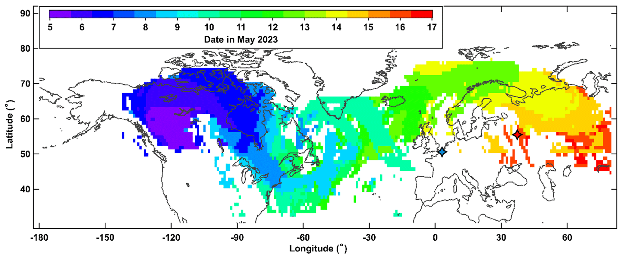
Figure 2 Spatiotemporal evolution of the smoke plume from the wildfire event in Alberta, Canada, on 5 May 2023. Color-filled time-coded areas indicate the Aerosol Index (AI) values from the OMPS NPP instrument exceeding 0.5. The blue- and red-filled stars indicate the location of Lille and Moscow lidar stations, respectively.

3.1 Variability in fluorescence depolarization ratio

At the first stage of our research we focused on the variability in the fluorescence depolarization ratio for aerosol types. The main attention was paid to smoke particles because they provide the strongest impact on the water vapor Raman measurements due to their high fluorescence capacity (Veselovskii et al., 2022).

Spatiotemporal distributions of the aerosol elastic and fluorescence backscattering coefficients (β₅₃₂ and β_F), on the night of 26–27 June 2023, are shown in Fig. 3. A dense smoke layer with β_F as high as $\mathrm{7.0}\times {\mathrm{10}}^{-\mathrm{4}}$ Mm⁻¹ sr⁻¹ occurred within the 4.0–10.0 km height range. The HYSPLIT back trajectories show that the air masses were transported from North America. The relative humidity increased from 40 % at 4 km to > 90 % at 7 km, where the formation of ice crystals started. Vertical profiles of aerosol elastic and fluorescence backscattering coefficients (β₅₃₂ and β_F), together with fluorescence capacity, are shown in Fig. 3c. Inside the smoke layer, G_F is about $\mathrm{3}\times {\mathrm{10}}^{-\mathrm{4}}$, which is a typical value for smoke (Veselovskii et al., 2022), whereas, above 6 km, it decreases due to ice formation. The presence of ice crystals increased the particle depolarization ratio δ₅₃₂ from 3 % at 6 km to 20 % at 8 km. Fluorescence signals are strongly depolarized. Inside the PBL, δ_F was about 60 % whereas above 2 km it dropped to approximately 45 %. The processes of hygroscopic growth and ice formation do not provide a noticeable impact on the δ_F value. During May–June observations, the depolarization ratio of smoke varied mainly inside the 45 %–55 % range.

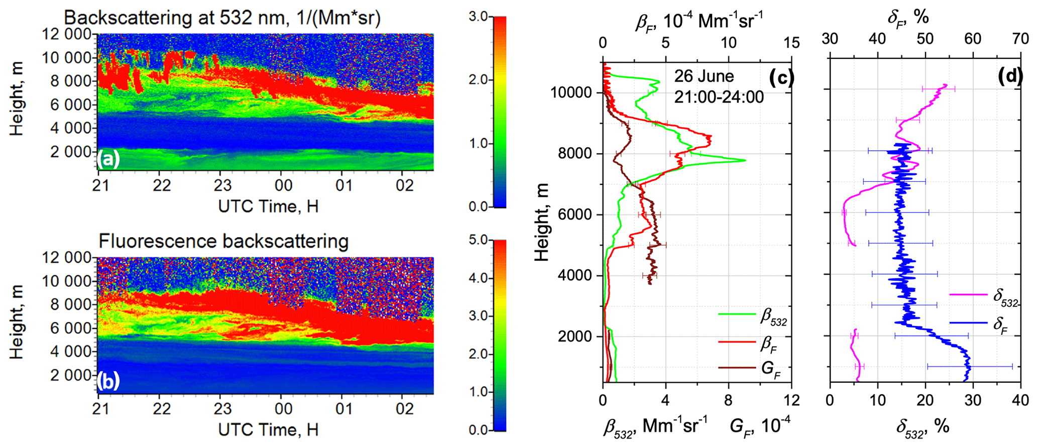
Figure 3 Smoke event on the night of 26–27 June 2023 over Lille. Spatiotemporal distributions of (a) aerosol backscattering coefficient β₅₃₂ and (b) fluorescence backscattering β_F (in 10⁻⁴ Mm⁻¹ sr⁻¹). Vertical profiles of (c) the aerosol β₅₃₂ and fluorescence β_F backscattering coefficients and the fluorescence capacity G_F, as well as (d) the particle δ₅₃₂ and the fluorescence δ_F depolarization ratios.

As discussed in our previous publications (Veselovskii et al., 2022; Hu et al., 2022), the fluorescence capacity of aged smoke varies inside the (2.5–5.5) $\times {\mathrm{10}}^{-\mathrm{4}}$ range, probably due to the changes in smoke composition and conditions of atmospheric transport. However, during the Alberta fires, several smoke plumes with high G_F have been observed. The highest fluorescence capacity was observed on the night of 16–17 June 2023. Vertical profiles of the aerosol properties for this episode are shown in Fig. 4. A dense smoke layers with fluorescence backscattering exceeding $\mathrm{10.0}\times {\mathrm{10}}^{-\mathrm{4}}$ Mm⁻¹ sr⁻¹ occurred within the 7.0–9.0 km height range. In this case, the maximal value of the fluorescence capacity reached $\mathrm{10.0}\times {\mathrm{10}}^{-\mathrm{4}}$. The fluorescence depolarization ratio was measured about 50 % through the entire smoke layer, and the process of ice formation (just like in Fig. 3d) does not influence δ_F. Thus, in May–June 2023 strong variations in G_F in the (2.5–10.0) $\times {\mathrm{10}}^{-\mathrm{4}}$ range were accompanied by relatively small variations in δ_F remaining in the 45 %–55 % interval.

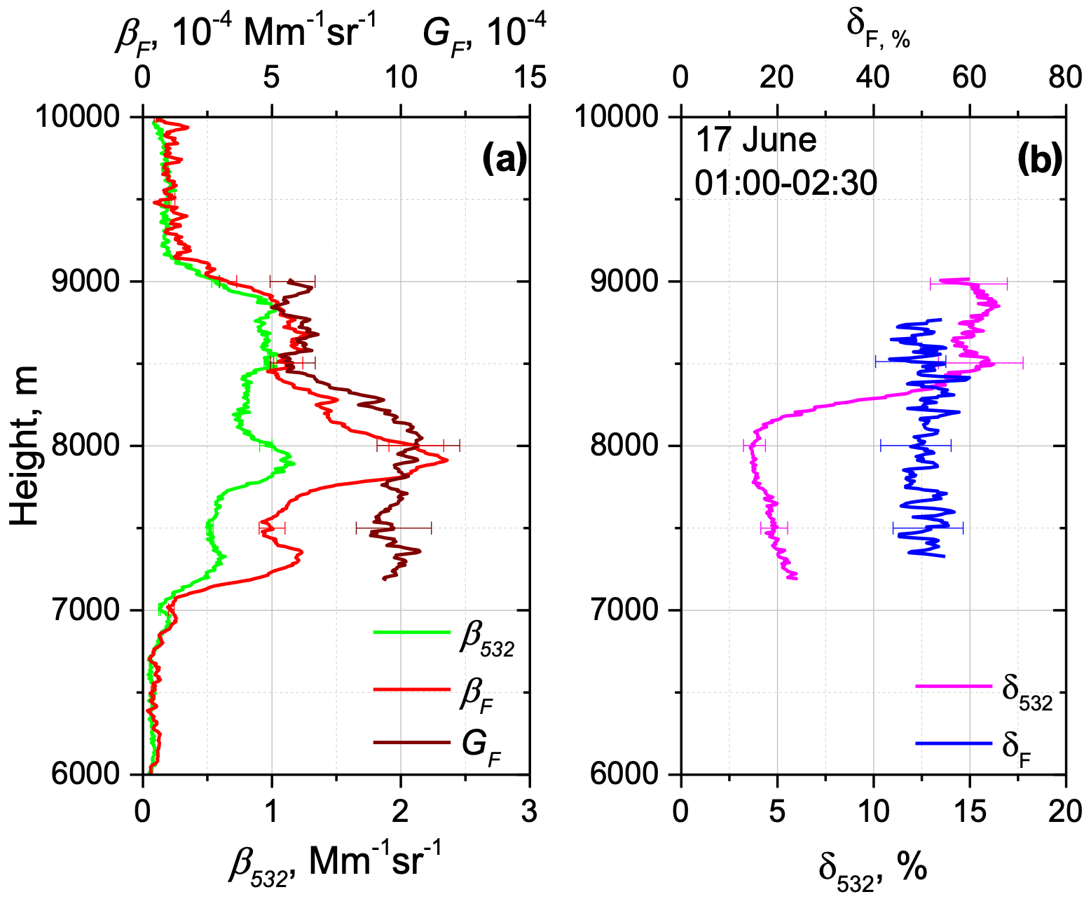
Figure 4 Vertical profiles of (a) aerosol β₅₃₂ and fluorescence β_F backscattering coefficients, fluorescence capacity G_F, and (b) particle δ₅₃₂ and fluorescence δ_F depolarization ratios on the night of 16–17 June 2023 for the period 01:00–02:30 UTC over Lille.

It is known that in the UTLS smoke particles can reach a depolarization ratio, δ₅₃₂, as high as 15 %–20 % (Burton et al., 2015; Haarig et al., 2018; Hu et al., 2019; Baars et al., 2019; Ohneiser et al., 2020). High values of the particle depolarization ratio are usually attributed to the complex internal structure of smoke particles (Mishchenko et al., 2016). Two smoke events in the UTLS, characterized by enhanced δ₅₃₂ on 28–29 May and 3–4 June 2023, are illustrated in Fig. 5. On 28–29 May, three smoke layers, at ∼ 3.5, 6.5 and 11.5 km, can be distinguished. High depolarization ratios, reaching 40 % at altitudes of 9.8–10.5 km, are due to ice clouds. In the lower smoke plumes ranging between 3.5 and 6.5 km, the particle depolarization did not exceed 8 %, whereas above 11 km δ₅₃₂ increased to 15 %. High values of δ₅₃₂ observed in the UTLS correlate with an increase in G_F and with fluorescence depolarization, δ_F, up to $\mathrm{7.0}\times {\mathrm{10}}^{-\mathrm{4}}$ and 70 %, respectively. Similar behavior was observed on 3–4 June, when the depolarization ratio, δ₅₃₂, above 11.5 km increased up to 15 %, simultaneously with an increase in G_F and δ_F up to $\mathrm{9.5}\times {\mathrm{10}}^{-\mathrm{4}}$ and 70 %, respectively. Thus, the change in particle morphology may affect the depolarization ratio at the fluorescence channel. Another possibility is that, in the UTLS, not only the particle structure can change, but the composition can as well. At the current stage of analysis, we are not yet able to draw conclusions about the mechanisms explaining the increase in fluorescence depolarization in the UTLS.

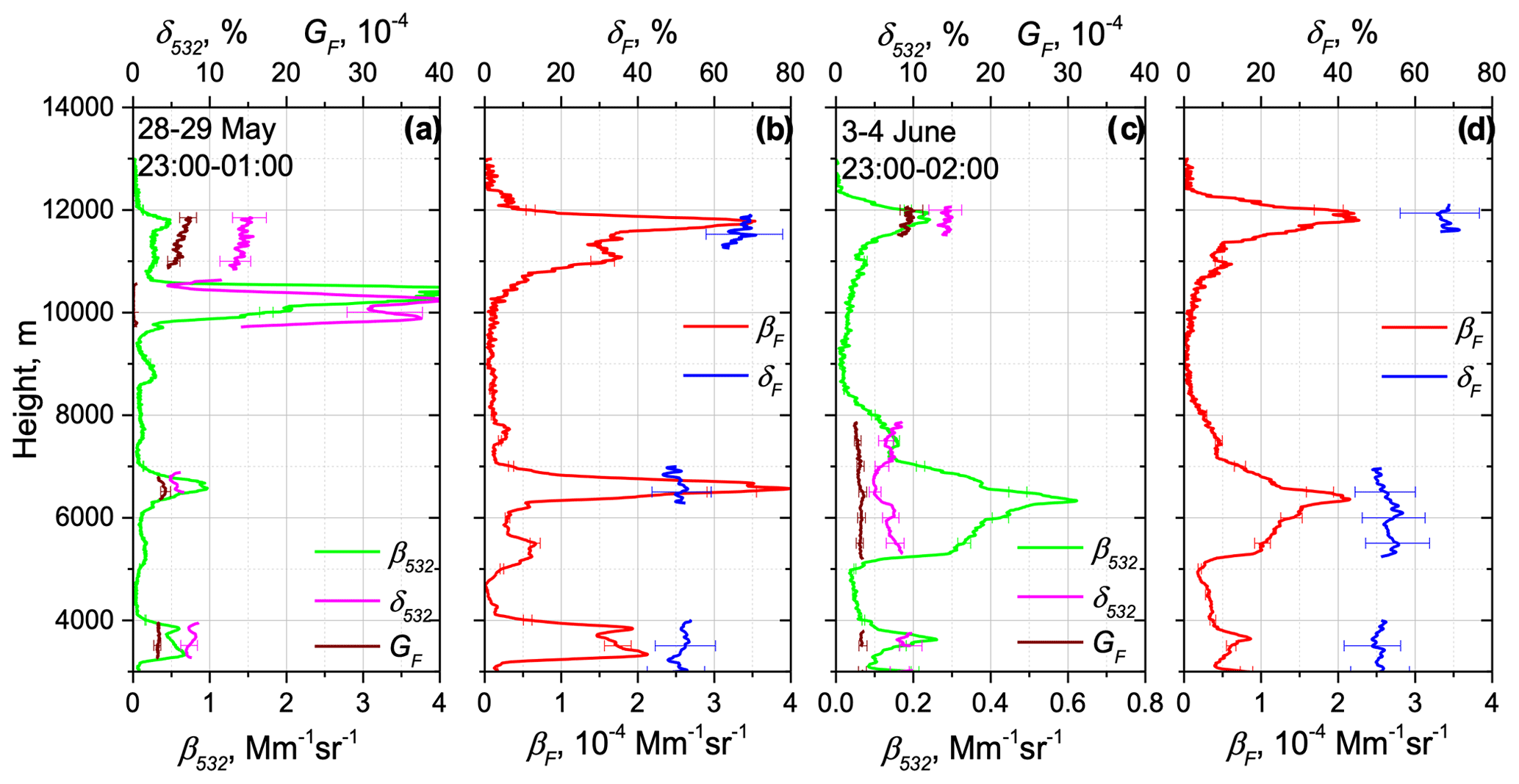
Figure 5 Vertical profiles of (a, c) backscattering coefficient β₅₃₂, particle depolarization ratio δ₅₃₂ and fluorescence capacity G_F, as well as (b, d) fluorescence backscattering β_F and fluorescence depolarization ratio δ_F, for two smoke episodes on the nights of 28–29 May and 3–4 June 2023 over Lille.

Furthermore, we did not observe the effect of atmospheric humidity on smoke fluorescence depolarization. However, inside the PBL the observed hygroscopic growth was accompanied by an increase in δ_F. During the 9–16 June 2023 period numerous particle hygroscopic growth cases were observed in the PBL. One such case, on the night of 12–13 June, is shown in Fig. 6. The relative humidity increased inside the PBL from 50 % to 90 % causing an increase in β₅₃₂ near the PBL top. Depolarization ratio δ₅₃₂ decreased with height, since the particles in the process of hygroscopic growth became more spherical. The fluorescence depolarization ratio, however, increased inside the PBL from 50 % to 70 %.

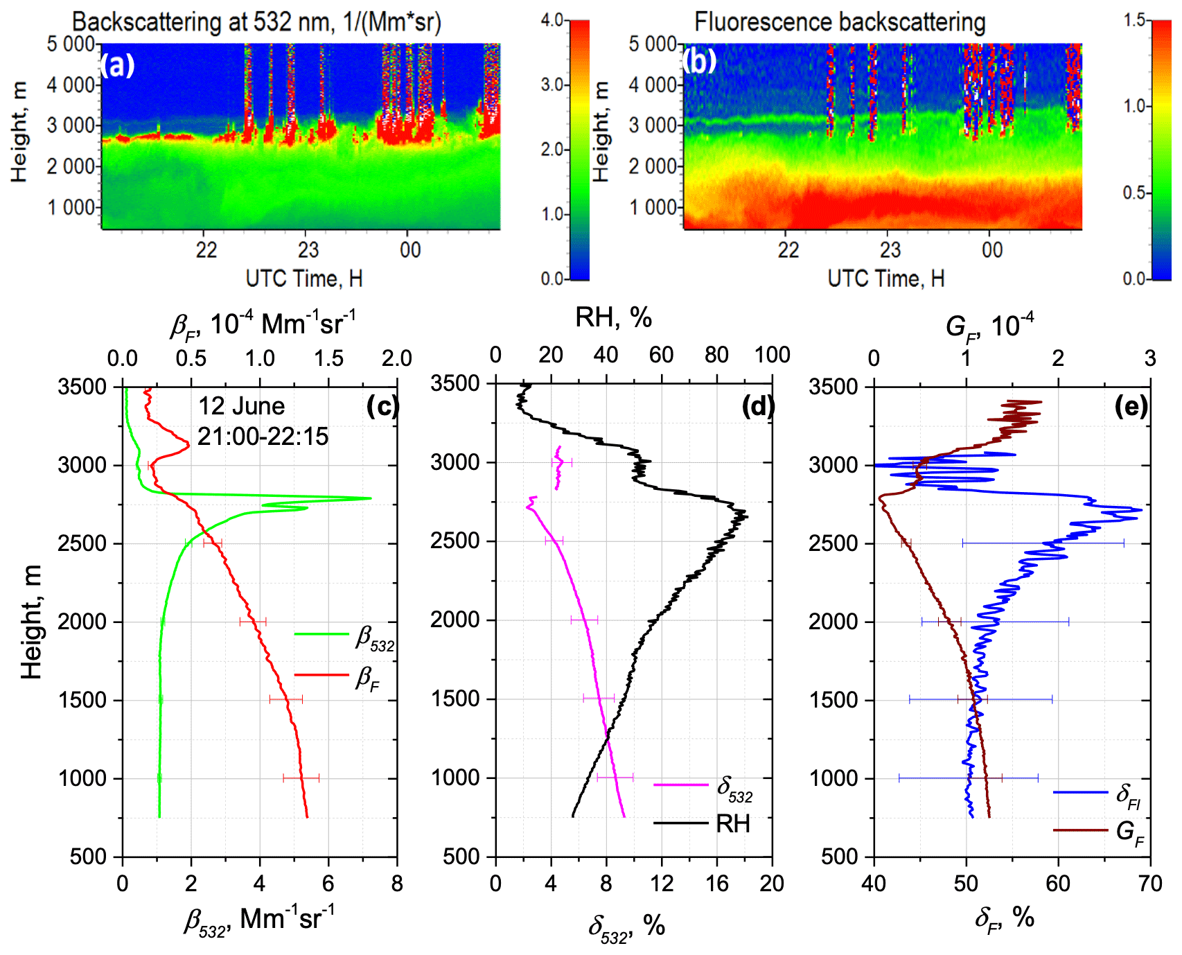
Figure 6 Particle hygroscopic growth in the PBL on the night of 12–13 June 2023 over Lille. Spatiotemporal distributions of (a) aerosol backscattering coefficient β₅₃₂ and (b) fluorescence backscattering β_F (in 10⁻⁴ Mm⁻¹ sr⁻¹). Vertical profiles of (c) aerosol β₅₃₂ and fluorescence β_F backscattering coefficients, (d) particle depolarization ratio δ₅₃₂ and the relative humidity RH, and (e) fluorescence depolarization ratio δ_F and fluorescence capacity G_F for the time period 21:00–22:15 UTC.

All results obtained during 9–16 June, showing the dependence of δ_F and δ₅₃₂ on the relative humidity, are summarized in Fig. 7. Particle depolarization δ₅₃₂ systematically decreased with relative humidity (RH), but, on 16 June, this dependence was not monotonic, which could be due to the change in aerosol composition with height. At low RH (below 30 %), the fluorescence depolarization ratio was about 50 %. However, at RH of about 90 %, δ_F increased up to 70 %. One of the possible explanations for that behavior could be an increase in rotational mobility of the molecules in the process of particle water uptake.

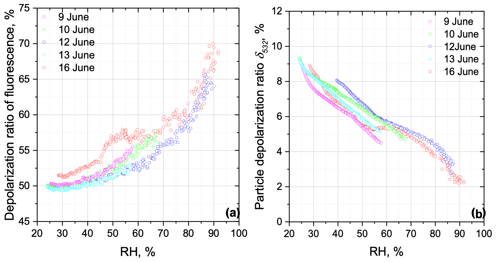
Figure 7 (a) Fluorescence depolarization ratio and (b) particle depolarization ratio δ₅₃₂ as a function of the relative humidity in the PBL for the measurements on 9, 10, 12, 13 and 16 June 2023 over Lille.

3.2 Fluorescence spectrum sampled with a five-channel lidar

The results presented in the previous section were obtained with a single-channel fluorescence lidar. However, for analyzing the variability in smoke properties (for example, increase in the fluorescence capacity with height), it is important to have information about a wider fluorescence spectrum. Moreover, to estimate the fluorescence contamination in the water vapor Raman channel, a relationship between fluorescence backscattering at 466 and 408 nm is used. Thus, we need to know the variability in the fluorescence spectrum in the short wavelength region. In our recent work (Veselovskii et al., 2023) we presented the first results obtained with a five-channel fluorescence lidar in operation at the GPI. This lidar is able to measure the fluorescence backscattering profiles at five spectral intervals centered at 438, 472, 513, 560 and 614 nm. During May–June 2023, several smoke plumes originating from Alberta fires were transported over Moscow. Although Lille and Moscow are very distant from each other (above 2200 km), the smoke plumes observed have the same origin; hence the fluorescence spectra measured over Moscow are quite helpful for the analysis of the Lille data.

Figure 8a, b and c present the fluorescence spectral backscattering coefficients, B_λ, for three smoke events detected in the UTLS above 10, 8 and 10 km for 15 May, 31 May and 20 June 2023, respectively. On 15 and 31 May smoke layers were also present inside the 4–6 km range. Inside the PBL the strongest fluorescence was systematically detected at the 438 nm channel, while, at higher altitudes, the maxima shifted to 560 nm. As follows from Figs. 8d–f, the ratio $B_{\mathrm{560}}/B_{\mathrm{438}}$ remained in the range 0.4–0.7 inside the PBL, whereas this ratio increased above 2.0 in the UTLS. Thus, for smoke events the maxima of the fluorescence spectrum shifted with height towards longer wavelengths. The ratio $B_{\mathrm{513}}/{\mathit{\beta }}_{\mathrm{355}}$ also increased with height, and, above 10 km, it reached the values of $\mathrm{1}\times {\mathrm{10}}^{-\mathrm{5}}$ nm⁻¹. In the UTLS, the maximal fluorescence capacity, G_F, measured by LILAS at 466 nm (with 44 nm bandwidth filter) was about $\mathrm{10}\times {\mathrm{10}}^{-\mathrm{4}}$. In the smoke layer, the ratio of backscattering coefficients ${\mathit{\beta }}_{\mathrm{355}}/{\mathit{\beta }}_{\mathrm{532}}$ is about 2, so the maximal ratio $B_{\mathrm{466}}/{\mathit{\beta }}_{\mathrm{355}}$ derived from LILAS measurements was about $\mathrm{1.1}\times {\mathrm{10}}^{-\mathrm{5}}$ nm⁻¹. Thus, values obtained over Lille and over Moscow are in good agreement.

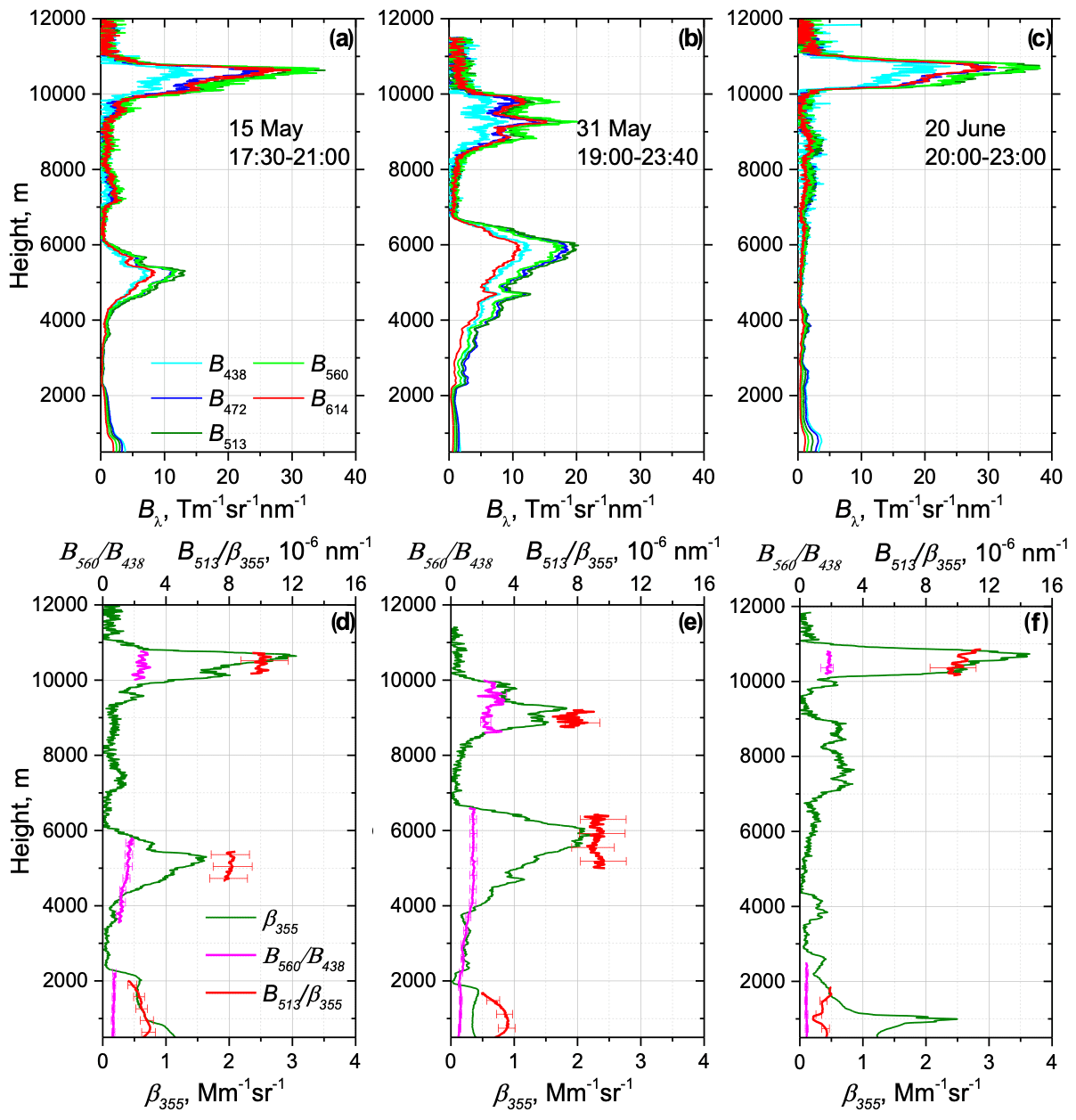
Figure 8 Fluorescence measurements over Moscow on 15 May, 31 May and 20 June 2023. Vertical profiles of (a–c) fluorescence spectral backscattering coefficients B_λ at 438, 472, 513, 560 and 614 nm and (d–f) aerosol backscattering coefficient β₃₅₅, the ratio $B_{\mathrm{560}}/B_{\mathrm{438}}$ and the ratio $B_{\mathrm{513}}/{\mathit{\beta }}_{\mathrm{355}}$. Measurements were performed at an angle of 48^∘ to the horizon.

The fluorescence spectra obtained for the above-mentioned smoke plumes are shown in Fig. 9. The values of B_λ are normalized to B₄₃₈. Inside the PBL, the maximum of fluorescence was measured at 438 nm, and it decreased with wavelength. In the smoke layers within 4–6 km, the maximum of fluorescence is observed at 513 nm, while, in the UTLS, the maximum shifted to 560 nm.

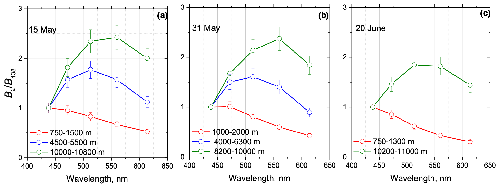
Figure 9 Fluorescence spectra $B_{\mathit{\lambda }}/B_{\mathrm{438}}$ at different height intervals measured during smoke episodes on 15 May, 31 May and 20 June 2023 over Moscow for the same temporal intervals as in Fig. 8.

When applying Eq. (19) to estimate the contribution of smoke fluorescence into the water vapor Raman channel of LILAS, we assumed that the ratio of the fluorescence backscattering at 466–408 nm ($B_{\mathrm{466}}/B_{\mathrm{408}}$) was constant. For the lidar in operation at GPI, the shortest available wavelength was 438 nm; therefore, at least, one can estimate the variability in the ratio $B_{\mathrm{472}}/B_{\mathrm{438}}$. Figure 10 presents the vertical profiles of $B_{\mathrm{472}}/B_{\mathrm{438}}$ for 11 smoke events occurring during the 15 May–20 June 2023 period. Inside the PBL, this ratio varied in the 0.6–1.0 range. The lowest values correspond to urban aerosols, while values of $B_{\mathrm{472}}/B_{\mathrm{438}}$ close to 1.0 probably indicate the presence of smoke particles inside the PBL. Smoke layers were observed mainly above 4.0 km and $B_{\mathrm{472}}/B_{\mathrm{438}}$ showed a tendency to increase in the UT. It is interesting that, for the period 15 May–1 June, the ratio was close to 1.5, whereas after 1 June, it became close to 1.0, which can be related to changes in the smoke source. The mean value of $B_{\mathrm{472}}/B_{\mathrm{438}}$ in the 4.0–11.0 km range over all observations is 1.38 with a standard deviation of 0.23 (relative variation is about 17 %). For the 466 and 408 nm channels the wavelength separation is larger, so one can expect a variation in $B_{\mathrm{466}}/B_{\mathrm{408}}$ in the smoke layer to be above that value. It points out the difficulties faced when the estimation of the fluorescence contamination in the water vapor Raman channel is performed from a single fluorescence channel at 466 nm. This issue was also discussed by Reichardt et al. (2023).

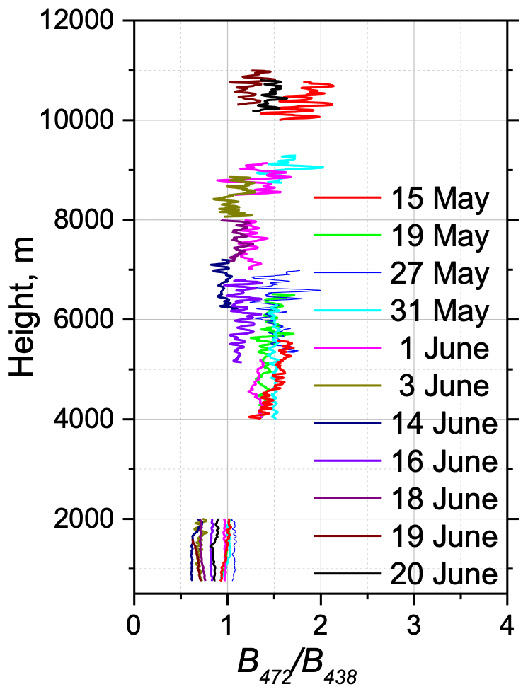
Figure 10 Height profiles of the ratio $B_{\mathrm{472}}/B_{\mathrm{438}}$ for smoke episodes during 15 May–20 June 2023 over Moscow. Smoke layers start above 4 km and go up to 11 km.

3.3 Estimation of fluorescence impact on water vapor Raman measurements

Measuring the depolarization ratio at the water vapor Raman channel provides an opportunity to control/evaluate the presence of a fluorescence leak in this channel. These depolarization measurements were performed over Lille during May–June 2023. Vertical profiles of water vapor depolarization ratio ${\stackrel{\mathrm{̃}}{\mathit{\delta }}}_{\mathrm{W}}$, together with ${\stackrel{\mathrm{̃}}{n}}_{\mathrm{W}}$, β₅₃₂, β_F and G_F, are shown in Fig. 11 for the nights of 8–9 and 10–11 June 2023. On 8–9 June the aerosols were confined mainly below 5 km. The fluorescence capacity was about $\mathrm{1.0}\times {\mathrm{10}}^{-\mathrm{4}}$ below 3.0 km, but above, G_F increased up to $\mathrm{2.5}\times {\mathrm{10}}^{-\mathrm{4}}$, indicating the presence of smoke particles. The depolarization ratio in the water vapor channel was about 2 % in the height range 1.5–3.5 km, where the values of ${\stackrel{\mathrm{̃}}{\mathit{\delta }}}_{\mathrm{W}}$ ranging within 1.8 %–2.0 % were observed at this height range, where the contribution of fluorescence was insignificant. The depolarization ratio δ_W was low because the interference filter at the water vapor channel selects only the strongest Q-branch lines and most of the rotational lines are blocked. The contribution of fluorescence becomes noticeable above 3.5 km where n_W dropped, resulting in an increase in ${\stackrel{\mathrm{̃}}{\mathit{\delta }}}_{\mathrm{W}}$ of up to ∼ 3 %. Below 1 km height we also observed an increase in ${\stackrel{\mathrm{̃}}{\mathit{\delta }}}_{\mathrm{W}}$ up to 2.2 %, where fluorescence backscattering is enhanced. Similar values of ${\stackrel{\mathrm{̃}}{\mathit{\delta }}}_{\mathrm{W}}$ were observed on 10–11 June, where the depolarization ratio increased up to 2.5 % inside the smoke layer observed at ∼ 3.75 km and below 2.0 km.

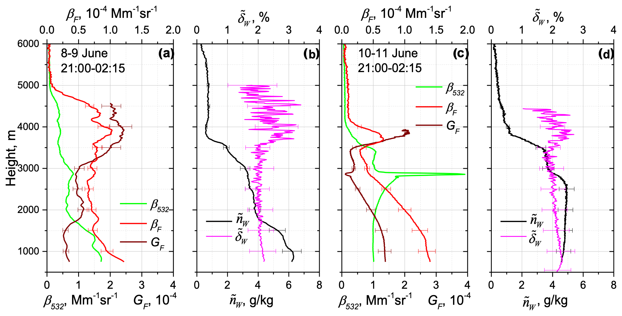
Figure 11 Impact of the aerosol fluorescence on the depolarization ratio in the water vapor Raman channel on the nights of 8–9 and 10–11 June 2023 over Lille. Vertical profiles of (a, c) particle backscattering β₅₃₂, fluorescence backscattering β_F and fluorescence capacity G_F, as well as (b, d) depolarization ratio ${\stackrel{\mathrm{̃}}{\mathit{\delta }}}_{\mathrm{W}}$ of the water vapor Raman signal and the water vapor mixing ratio ${\stackrel{\mathrm{̃}}{n}}_{\mathrm{W}}$.

As discussed in Sect. 2.2, the contribution of fluorescence to the WVMR channel can be derived from Eq. (20) if ${\stackrel{\mathrm{̃}}{\mathit{\delta }}}_{\mathrm{W}}$ and δ_F are measured simultaneously. Figure 12 presents the modeling of the relative error $\frac{\mathrm{\Delta }{n}_{\mathrm{W}}}{{\stackrel{\mathrm{̃}}{n}}_{\mathrm{W}}}$ introduced by the fluorescence to the WVMR channel as a function of ${\stackrel{\mathrm{̃}}{\mathit{\delta }}}_{\mathrm{W}}$. The computations are performed for different fluorescence depolarization ratios δ_F= 50 %, 60 % and 70 % to include both smoke and urban particles. A depolarization ratio in the water vapor Raman channel in the absence of fluorescence was assumed to be δ_W= 2 %. For a depolarization ratio ${\stackrel{\mathrm{̃}}{\mathit{\delta }}}_{\mathrm{W}}$ below 3 % the relative error $\frac{\mathrm{\Delta }{n}_{\mathrm{W}}}{{\stackrel{\mathrm{̃}}{n}}_{\mathrm{W}}}$ did not exceed 3 %. As follows from the fluorescence spectra in Fig. 9, the fluorescence of urban particles increases towards shorter wavelengths; thus, one can expect an impact of the urban aerosol fluorescence on the water vapor measurements. In practice, however, we did not observe values of ${\stackrel{\mathrm{̃}}{\mathit{\delta }}}_{\mathrm{W}}$ exceeding 3 % in the PBL; thus, the contribution of aerosol in the PBL is not critical. The reason is due to the low fluorescence capacity (about one order lower than that of smoke) and higher water vapor content compared to the free troposphere.

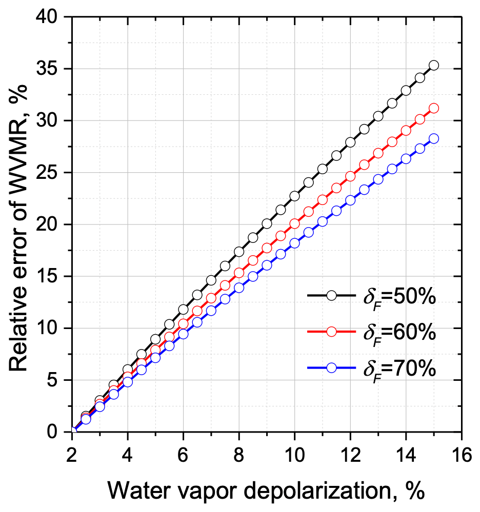
Figure 12 Relative error in water vapor mixing ratio (WVMR) $\frac{\mathrm{\Delta }{n}_{\mathrm{W}}}{{\stackrel{\mathrm{̃}}{n}}_{\mathrm{W}}}$ induced by the fluorescence as a function of depolarization ratio ${\stackrel{\mathrm{̃}}{\mathit{\delta }}}_{\mathrm{W}}$ in the water vapor Raman channel for three values of fluorescence depolarization ratio: δ_F= 50 %, 60 %, 70 %. The depolarization ratio of water vapor Raman backscatter in the absence of fluorescence is assumed to be δ_W= 2 %.

Vertical profiles of ${\stackrel{\mathrm{̃}}{\mathit{\delta }}}_{\mathrm{W}}$ shown in Fig. 11 become noisy at heights where n_W is low, and thus ${\stackrel{\mathrm{̃}}{\mathit{\delta }}}_{\mathrm{W}}$ cannot be used for the correction of the fluorescence effect in the upper troposphere. To overcome this, we derived the parameter η from Eq. (18) at low altitudes where ${\stackrel{\mathrm{̃}}{\mathit{\delta }}}_{\mathrm{W}}$ values are available, and, thus, these η values can be used to calculate Δn_W from Eq. (19) in the entire height range. In such an approach, however, one has to assume that the relationship between fluorescence cross sections at 466 and 408 nm remains constant with height. As discussed in Sect. 3.2, such an assumption can yield significant bias in the calculation of Δn_W, and, at this stage, we do not provide corrected profiles of the WVMR.

For the accurate calculation of η one needs smoke events with strongly enhanced ${\stackrel{\mathrm{̃}}{\mathit{\delta }}}_{\mathrm{W}}$ values, which are usually observed in the smoke layers with low WVMR. Such suitable events are shown on the nights of 26–27 May and 5–6 June 2023 in Fig. 13. On 26–27 May a smoke layer characterized by high fluorescence (β_F up to $\mathrm{5}\times {\mathrm{10}}^{-\mathrm{4}}$ Mm⁻¹ sr⁻¹) and low ${\stackrel{\mathrm{̃}}{n}}_{\mathrm{W}}$ (below 0.2 g kg⁻¹) values is observed at 3.5 km. The relevant fluorescence depolarization ratio was about 47 %, and ${\stackrel{\mathrm{̃}}{\mathit{\delta }}}_{\mathrm{W}}$ increased from 2 % up to 12 % in the middle of this layer. The parameter η calculated from Eq. (18) inside this smoke layer was about $\mathrm{2}\times {\mathrm{10}}^{-\mathrm{3}}$ (g kg⁻¹) (Mm⁻¹ sr⁻¹)⁻¹. On 5–6 June the depolarization ratio ${\stackrel{\mathrm{̃}}{\mathit{\delta }}}_{\mathrm{W}}$ in the smoke layer increased up to 10 %, and the value of η was very similar. The values of η derived for several smoke episodes varied in the range (2–2.5) $\times {\mathrm{10}}^{-\mathrm{3}}$ (g kg⁻¹) (Mm⁻¹ sr⁻¹)⁻¹. To estimate Δn_W we used the mean value of $\mathit{\eta }=\mathrm{2.25}\times {\mathrm{10}}^{-\mathrm{3}}$ (g kg⁻¹) (Mm⁻¹ sr⁻¹)⁻¹, which is suitable only for smoke, while for particles in the PBL, η can have a different value. However, in the PBL, the low depolarization ratios of ${\stackrel{\mathrm{̃}}{\mathit{\delta }}}_{\mathrm{W}}$ prevented us from calculating η.

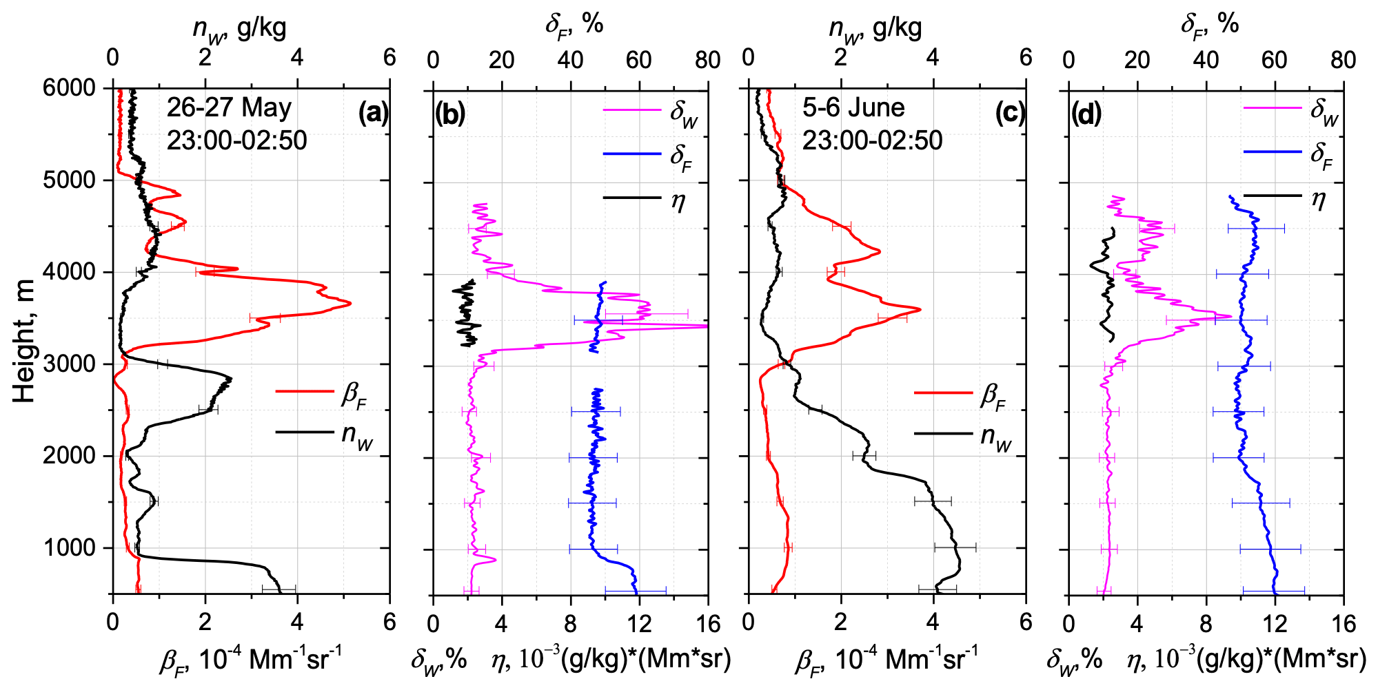
Figure 13 Fluorescence measurements over Lille on the night of 26–27 May and 5–6 June 2023. (a, c) Vertical profiles of the fluorescence backscattering β_F, the water vapor mixing ratio ${\stackrel{\mathrm{̃}}{n}}_{\mathrm{W}}$, (b, d) the depolarization ratio of the water vapor Raman signal ${\stackrel{\mathrm{̃}}{\mathit{\delta }}}_{\mathrm{W}}$, the fluorescence depolarization ratio δ_F and parameter η, describing the contribution of the fluorescence to the water vapor channel.

Figure 14 presents the vertical profiles of WVMR, the fluorescence backscattering and the error Δn_W introduced by the fluorescence in WVMR on 26–27 May, 28–29 May and 16–17 June. Smoke layers with strong fluorescence occurred systematically in our upper-tropospheric observations. The current LILAS system is not powerful enough to derive accurate water vapor measurements above 10 km; however, an increase in ${\stackrel{\mathrm{̃}}{n}}_{\mathrm{W}}$ in the fluorescent smoke layers is visible. Remember that Eq. (19) for Δn_W contains the factor $\frac{\mathrm{1}}{n_{\mathrm{R}}}$ (inverse relative change in nitrogen number density); thus, the fluorescence impact on WVMR will increase with height. The uncertainties $\frac{\mathrm{\Delta }{n}_{\mathrm{W}}}{{\stackrel{\mathrm{̃}}{n}}_{\mathrm{W}}}$ for all events considered are shown in Fig. 14d. On 26–27 and 28–29 May the uncertainty of $\frac{\mathrm{\Delta }{n}_{\mathrm{W}}}{{\stackrel{\mathrm{̃}}{n}}_{\mathrm{W}}}$ at 11 km is of the order of 100 %. On 16 June the smoke layer is lower (at 9 km), and the uncertainty is about 50 %. Our demonstration shows that smoke fluorescence can significantly impact the water vapor measurements. The proposed approach, based on the analysis of the depolarization ratio of the water vapor signal, has the potential for the estimation and correction of this impact.

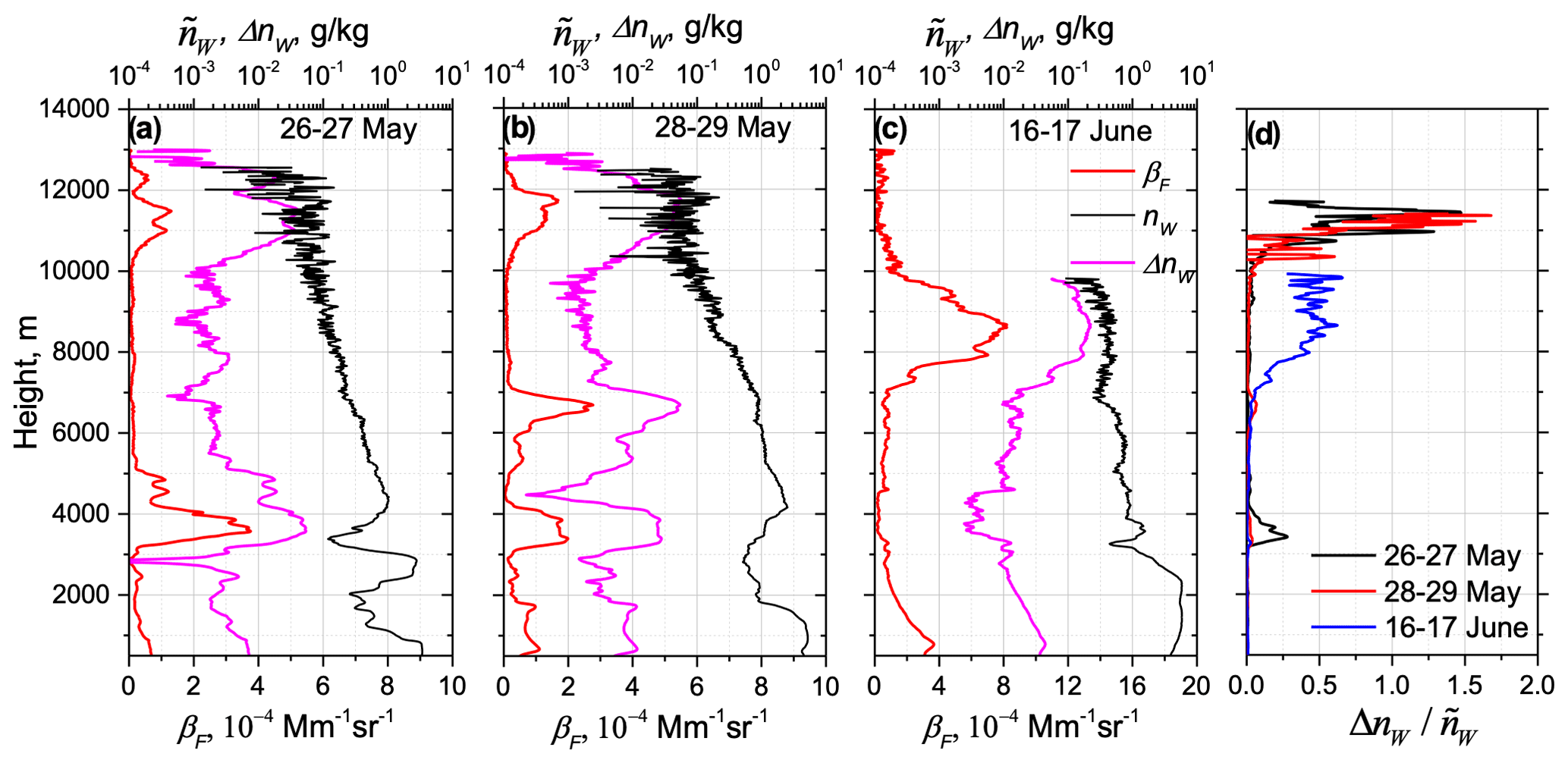
Figure 14 Impact of smoke fluorescence on the water vapor measurements. Vertical profiles of the fluorescence backscattering β_F, water vapor mixing ratio ${\stackrel{\mathrm{̃}}{n}}_{\mathrm{W}}$ and bias in water vapor channel Δn_W provided by the fluorescence of smoke for episodes on the nights of (a) 26–27 May, (b) 28–29 May and (c) 16–17 June 2023 for the time interval 21:00–02:30 UTC over Lille. (d) Error $\frac{\mathrm{\Delta }{n}_{\mathrm{W}}}{{\stackrel{\mathrm{̃}}{n}}_{\mathrm{W}}}$ introduced by smoke fluorescence for the three episodes.

4 Conclusion

This study is one of the first efforts to measure the depolarization ratio of the fluorescence of the atmospheric aerosols. Analysis of more than 30 spring and summer smoke events allows the evaluation of the main aerosol intensive properties, including fluorescence capacity and the particle and fluorescence depolarization ratios. The fluorescence capacity of smoke in the troposphere varied within (2.5–10.0) $\times {\mathrm{10}}^{-\mathrm{4}}$; however, in spite of strong G_F variation, δ_F remained within a relatively narrow interval of 45 %–55 %. Additional observations revealed that for smoke plumes in the upper troposphere the fluorescence depolarization ratio increased up to 70 %. At the moment, we cannot fully explain the mechanism responsible for this δ_F increase. It can be related to complex particle internal structure at high altitudes, as well as to the change in the chemical composition, revealed by the shift in the maximum of the fluorescence spectra to longer wavelengths in the upper troposphere (Fig. 9).

Inside the PBL, the fluorescence depolarization ratio was higher than that of smoke and varied within the 50 %–70 % range. Moreover, the fluorescence depolarization ratio of urban particles strongly depends on the relative humidity, and, in contrast to the elastic scattering, the depolarization of fluorescence increases with RH. One possible origin of this phenomena could be attributed to an increase in the rotational mobility of the molecules involved in the process of water uptake.

The depolarization ratio of the water vapor Raman backscatter, in the absence of fluorescence, appeared to be quite low (${\mathit{\delta }}_{\mathrm{W}}=\mathrm{2}\pm \mathrm{0.5}$ %). As a result, the depolarization ratio of the water vapor Raman backscatter is sensitive to the presence of strongly depolarized fluorescence signals, and the contribution of fluorescence to the WVMR can be calculated from the measured value ${\stackrel{\mathrm{̃}}{\mathit{\delta }}}_{\mathrm{W}}$. However, with the lidar used in this work, measurements of ${\stackrel{\mathrm{̃}}{\mathit{\delta }}}_{\mathrm{W}}$ are only possible up to the middle troposphere, while the problem of the fluorescence interference is the most crucial in UTLS. To estimate the impact of fluorescence on the WVMR in UTLS, the height-independent parameter η, linking fluorescence at 466 and at 408 nm, was used. Such an approach relies on the assumption that η remains constant and allows only a rough estimation of the correction term for the WVMR, Δn_W. One possible solution to increase the accuracy of Δn_W is to implement an additional shorter wavelength channel (438 nm or even shorter). Another technical approach worth considering is equipping the 408 nm channel with a polarizing cube, given the low depolarization ratio of Raman water vapor backscatter. Thus, the depolarized channel at 408 nm can be used for fluorescence measurements. As the polarizing cubes work in a wide spectral range, one can select a spectral region outside of the water vapor spectrum (400–418 nm) for fluorescence monitoring. We plan this experiment, as well as other innovative approaches, with our future high-power fluorescence lidar, LIFE (Laser Induced Fluorescence Explorer), whose start of operation is scheduled for the beginning of 2024.