A method for estimating localized CO₂ emissions from co-located satellite XCO₂ and NO₂ images

Carbon dioxide (CO₂) is the most important anthropogenic greenhouse gas. Its atmospheric concentration has increased by almost 50 % since the beginning of the industrial era, causing climate change. Fossil fuel combustion is responsible for most of the atmospheric CO₂ increase, which originates to a large extent from localized sources such as power stations. Independent estimates of the emissions from these sources are key to tracking the effectiveness of implemented climate policies to mitigate climate change. We developed an automatic procedure to quantify CO₂ emissions from localized sources based on a cross-sectional mass-balance approach and applied it to infer CO₂ emissions from the Bełchatów Power Station (Poland) using atmospheric observations from the Orbiting Carbon Observatory 3 (OCO-3) in its snapshot area map (SAM) mode. As a result of the challenge of identifying CO₂ emission plumes from satellite data with adequate accuracy, we located and constrained the shape of emission plumes using TROPOspheric Monitoring Instrument (TROPOMI) NO₂ column densities. We automatically analysed all available OCO-3 overpasses over the Bełchatów Power Station from July 2019 to November 2022 and found a total of nine that were suitable for the estimation of CO₂ emissions using our method. The mean uncertainty in the obtained estimates was 5.8 Mt CO₂ yr⁻¹ (22.0 %), mainly driven by the dispersion of the cross-sectional fluxes downwind of the source, e.g. due to turbulence. This dispersion uncertainty was characterized using a semivariogram, made possible by the OCO-3 imaging capability over a target region in SAM mode, which provides observations containing plume information up to several tens of kilometres downwind of the source. A bottom-up emission estimate was computed based on the hourly power-plant-generated power and emission factors to validate the satellite-based estimates. We found that the two independent estimates agree within their 1σ uncertainty in eight out of nine analysed overpasses and have a high Pearson's correlation coefficient of 0.92. Our results confirm the potential to monitor large localized CO₂ emission sources from space-based observations and the usefulness of NO₂ estimates for plume detection. They also illustrate the potential to improve CO₂ monitoring capabilities with the planned Copernicus Anthropogenic CO₂ Monitoring (CO2M) satellite constellation, which will provide simultaneously retrieved XCO₂ and NO₂ maps.

1 Introduction

CO₂ is the most important anthropogenic greenhouse gas, and its cumulative atmospheric concentration increase plays a major role in global warming and climate change (Chen et al., 2021). In 2015, the Paris Agreement was adopted to limit global warming to well below 2 ^∘C and pursue “efforts to limit the temperature increase to 1.5 ^∘C above pre-industrial levels” (UNFCCC, 2015). To meet these objectives, net greenhouse gas emissions need to be rapidly reduced (IPCC, 2023; Rockström et al., 2017). Under this agreement and as part of the mitigation strategy, the parties report their national greenhouse gas inventories, usually computed using bottom-up methods based on statistical activity data and emission factors (IPCC, 2006). Top-down approaches, based on atmospheric observations, can complement these inventories and verify their accuracy (Bergamaschi et al., 2018).

Most of the CO₂ emissions result from the combustion of fossil fuels. About one-third of the total fossil fuel emissions happen at localized sources, such as power plants (Oda and Maksyutov, 2011; IEA, 2019; Crippa et al., 2022). Therefore, monitoring the CO₂ emissions from these targets is key to tracking the correct application and effectiveness of the reduction policies and supporting the assessment of the global stocktake implemented by the United Nations. Satellite observations have the advantages of providing periodical data and having potential global coverage. Furthermore, as initially proposed by Bovensmann et al. (2010) and Velazco et al. (2011), analysis of space-based observations of XCO₂, the column-averaged dry-air mole fraction of CO₂, provides independent estimates of CO₂ emissions from localized sources like power plants (e.g. Reuter et al., 2019; Nassar et al., 2017, 2022.

The detection of CO₂ emission plumes from localized sources is challenging due to the small anomaly in XCO₂ due to these emissions in the atmosphere, which are typically in the order of 1 ppm and of the same order of magnitude as the instrument noise (Bovensmann et al., 2010). As net atmospheric CO₂ has a long lifetime, ranging from years to millennia (e.g. Ciais et al., 2013), and large fluxes of natural origin, these enhancements are also much smaller than CO₂ background values and natural variability. Therefore, to quantify the CO₂ emission plumes from localized sources, further assumptions are usually needed, e.g. a Gaussian plume shape considering steady state (e.g. Nassar et al., 2017).

Nitric oxide (NO) is co-emitted with CO₂ during the combustion of fossil fuels. It rapidly reacts with ozone (O₃) to form nitrogen dioxide (NO₂). During the day, NO₂ is photolysed to produce NO and atomic oxygen. Therefore, NO and NO₂ are coupled during the daytime, and their sum is referred to as NO_x. Unlike CO₂, NO_x has a lifetime in the order of hours in the daytime boundary layer. As a result, NO₂ vertical column densities in plumes released from fossil fuel combustion exceed background values and sensor noise, typically by orders of magnitude. This makes NO₂ a suitable tracer for recently emitted CO₂. The approach of using NO₂ as a proxy for recent CO₂ emissions for the combustion of fossil fuels has been successfully used previously, both to estimate the CO₂ emissions from NO_x-to-CO₂ emission ratios (e.g. Reuter et al., 2014; Hakkarainen et al., 2021) and to detect and constrain the spatial extent of the emission plume, using observed data (e.g. Reuter et al., 2019) as well as synthetic observations (e.g. Kuhlmann et al., 2019, 2021). The use of NO₂ as a proxy for CO₂ profits from less-noisy data at the expense of required knowledge about the source-dependent NO_x-to-CO₂ emission ratios as well as about the NO₂-to-NO_x ratios, which are determined by the chemistry of NO_x within the plume. A more cautious approach is the use of NO₂ to constrain the spatial extent of the emission plume, e.g. fitting simultaneously observations of NO₂ and CO₂ along a plume cross section, so that the width (and possibly the location) of the CO₂ is constrained by that of NO₂ (Reuter et al., 2019; Hakkarainen et al., 2023; Kuhlmann et al., 2021). This latter approach profits from simultaneous observations of both gases for an increased correlation in the spatial structures and is, therefore, less applicable in the case of significant changes in the meteorological conditions in the time between the CO₂ and NO₂ measurements. We investigated a technique based on NO₂ data to constrain the region containing the CO₂ emission plume without simultaneously fitting both datasets. We used currently available observations of XCO₂ and column densities of NO₂, retrieved from the Orbiting Carbon Observatory 3 (OCO-3) and the TROPOspheric Monitoring Instrument (TROPOMI), respectively. This is partly in preparation for the planned extensive exploitation of this approach to observations from the upcoming Copernicus Anthropogenic CO₂ Monitoring (CO2M) mission, which aims to quantify anthropogenic CO₂ emissions and will simultaneously retrieve XCO₂ and NO₂ column densities (Bézy et al., 2019). The CO2M builds on the heritage of the preparatory work undertaken in the CarbonSat concept studies (Buchwitz et al., 2013; Bovensmann et al., 2010) and the SCanning Imaging Absorption spectroMeter for Atmospheric CHartographY (SCIAMACHY) observations (Burrows et al., 1995; Bovensmann et al., 1999) on the European Space Agency (ESA) Environmental Satellite (ENVISAT), the Thermal And Near infrared Sensor for carbon Observations – Fourier Transform Spectrometer (TANSO-FTS) observations on the Greenhouse Gases Observing Satellite (GOSAT) (Kuze et al., 2009, 2016), and the Orbiting Carbon Observatory observations (Crisp et al., 2004; Eldering et al., 2019).

Several methods exist to quantify the emissions from localized sources using satellite data, as described by studies such as Varon et al. (2018). The Gaussian plume inversion method, based on the simulation of a Gaussian plume which is then fitted to the observations, has been used to quantify power plant emissions from both OCO-2 and OCO-3 data (Nassar et al., 2022, 2017; Chevallier et al., 2022). The Gaussian model describes a plume in steady state; therefore, it does not account for eddies but rather relies on the assumption that their effects are negligible for multi-kilometre spatial scales. We have used a mass-balance cross-sectional flux method on XCO₂ retrievals from OCO-3. The cross-sectional flux method, along with the imaging capabilities of OCO-3, allowed us to analyse plume structures and estimate the magnitude of random errors affecting the computed emission rate. A cross-sectional method was also used by Hakkarainen et al. (2023) to derive CO₂ emissions of localized sources in the South African Highveld from OCO-3 data. We focused on the Bełchatów Power Station (Poland), which is among the power plants with the highest CO₂ emissions in the world. This power station was also the object of the study by Nassar et al. (2022), who quantified its emissions using OCO-3 data.

This paper is structured as follows. Our cross-sectional flux method for the top-down quantification of the CO₂ emissions from localized sources is described in Sect. 2. The datasets used are presented in Sect. 2.1. The plume detection and characterization algorithm, based on TROPOMI NO₂ data, is described in Sect. 2.2.1. Section 2.2.2 describes the processing of the XCO₂ data to estimate the emission rate, as detailed in Sect. 2.2.3. The estimation of the uncertainties is explained in Sect. 2.3. We briefly describe the scene selection procedure (Sect. 2.5) and the method to compute bottom-up emission estimates (Sect. 2.6) to verify the top-down computed emission rates. Finally, the results are shown in Sect. 3 and discussed in Sect. 4 along with the conclusions.

2 Datasets and methods

2.1 Datasets

2.1.1 XCO₂

NASA's OCO-3 XCO₂ retrievals were the main input data used to derive the CO₂ emissions. NASA's OCO-3 instrument, located on board the International Space Station (ISS) since May 2019, measures reflected sunlight in three bands, centred on the molecular oxygen-A band at 0.76 µm and the two CO₂ bands at 1.6 and 2.0 µm. The instrument has eight footprints, each of 1.6 km, and it sweeps about 2.2 km in the 0.33 s integration time. As a result of the ISS precessing orbit, the local overpass time of OCO-3 varies each day and it views latitudes between approximately ±52^∘. In its snapshot area map (SAM) mode, it can scan almost adjacent swaths over CO₂ emission hotspots and other targets. These SAMs are scans of a region of about 80 km × 80 km, taken in approximately 2 min (Eldering et al., 2019; Payne et al., 2022).

We utilized observations taken in SAM mode from the Level-2 Lite XCO₂ OCO-3 product (Taylor et al., 2023; O’Dell et al., 2018) in its version 10.4r, based on the Atmospheric Carbon Observations from Space (ACOS) retrieval algorithm (O’Dell et al., 2012; Crisp et al., 2012). These XCO₂ estimates are geolocated, bias-corrected and contain a quality flag, which we have used to filter out estimates that are less likely to be accurate. This quality filtering is derived from thresholds on single retrieval variables that are identified to cause the largest differences in the retrieved XCO₂ compared with truth proxies (Payne et al., 2022; O’Dell et al., 2018).

2.1.2 NO₂

We used TROPOMI NO₂ retrievals to detect the shape and location of the NO₂ enhancement due to the power plant emission plume. TROPOMI, on board the ESA Sentinel-5 Precursor (S5P) satellite, provides observations on NO₂, among other atmospheric constituents (Veefkind et al., 2012). It has a swath of approximately 2600 km across the track of the satellite, divided into 450 ground pixels of about 5.6 km (along the track) × 3.6 km (across the track) at nadir. It has a nadir-viewing grating spectrometer with four detectors for the different spectral bands: UV and VIS (ultraviolet and visible, respectively, 270–500 nm), NIR (near-infrared, 710–770 nm), and SWIR (short-wave infrared, 2314–2382 nm) (Eskes et al., 2022). S5P has a sun-synchronous orbit with a mean local solar time at the ascending node of 13:30. It performs 14 orbits per day with a repeat cycle of 16 d, and its revisit time is approximately 1 d.

We used slant column densities (SCDs) obtained with a differential optical absorption spectroscopy (DOAS) retrieval in the region from 425 to 497 nm (Richter et al., 2011). The SCD of a trace gas is a measure of its density along the average light path from the Sun to the instrument after reflection at the Earth's surface. Consequently, it depends on the viewing and solar geometry, as well as on other factors like the presence of clouds and aerosols. The vertical column densities (VCDs) are related to SCDs via the air mass factor, AMF, as follows: VCD $=\frac{\text{SCD}}{\text{AMF}}$. The accuracy of the absolute VCDs is less relevant for our application, as we do not use them for emission quantification but rather for detecting enhanced anomalies with respect to background values and, thus, quantifying the spatial extent of the emission plume from a localized source. Therefore, we neglected multiple scattering in the atmosphere by the electromagnetic radiation in the spectral region used for the retrieval and approximated the VCDs considering a geometrical AMF from the viewing zenith angle (θ_v) and the solar zenith angle (θ_s) as follows: AMF $=\text{sec}{\mathit{\theta }}_{\mathrm{v}}+\text{sec}{\mathit{\theta }}_{\mathrm{s}}$.

2.1.3 Meteorological data

We obtained meteorological information from the ERA5 dataset, the fifth-generation atmospheric reanalysis of the global climate covering the period from 1940 to present (Hersbach et al., 2017, 2020), produced by the European Centre for Medium Range Weather Forecast (ECMWF) and provided by the Copernicus Climate Change Service (C3S). We used instantaneous hourly estimates of a number of atmospheric variables in a 0.25^∘ × 0.25^∘ grid and at 137 hybrid sigma-pressure vertical levels.

From ERA5, we obtained, for the different vertical layers, the horizontal wind speed components, u and v. We also computed the number of dry-air molecules in the vertical column from meteorological profiles. Assuming that the emission plume is well mixed within the boundary layer, we computed, at each location and time, an average of each wind component within the boundary layer weighted by the number of dry-air molecules in the corresponding vertical layer. Brunner et al. (2023) found, with their simulations over the Bełchatów and Jänschwalde power plants in May and June 2018 and in consistency with flight observations, that this assumption of a well-mixed emission plume within the boundary layer is a good approximation during the daytime.

2.2 Top-down CO₂ emission quantification method

We estimated the net emission rate, f, from a localized source using a cross-sectional flux method. This method is based on mass balance so that f is the flux through any cross section (CS) downwind of the source.

Let ρ (kg m⁻²) be a map of the CO₂ vertical column mass density at each spatial pixel and ρ_bg be the CO₂ vertical column mass density map for the background, i.e. the corresponding ρ in the absence of the source under analysis. The anomaly in the vertical column mass density, Δρ, resulting from the emissions of the source with emission rate f, is given by $\mathrm{\Delta }\mathit{\rho }=\mathit{\rho }-{\mathit{\rho }}_{\mathrm{bg}}$ at each spatial pixel. Let $\mathit{w}=(u,v)$ (m s⁻¹) be the horizontal wind vector field at plume height and let us consider a CS of infinite length (or whose length is larger than or equal to the plume width) through this map and downwind of the source, as sketched in Fig. 1. The normal vector to the CS, n, forms an angle θ with w. The mass flux density field is then given by F=wΔρ. Let us also consider a positively oriented closed curve C enclosing the emission source (and no other sources), with normal vector n_C at each point and with one side coincident to the CS. Under stationary conditions and assuming that all of the emitted CO₂ mass was transported downwind, the only non-zero flux through this curve is given by the flux through the CS, which is, by mass balance, a measure of the net emission rate:

$$\begin{array}{}\text{(1)}& f=\underset{\mathrm{C}}{\oint }\mathit{F}{\mathit{n}}_{\mathrm{C}}\mathrm{d}l=\underset{-\mathrm{\infty }}{\overset{+\mathrm{\infty }}{\int }}\mathit{F}\mathit{n}\mathrm{d}l=\underset{-\mathrm{\infty }}{\overset{+\mathrm{\infty }}{\int }}{w}_{⟂}\mathrm{\Delta }\mathit{\rho }\mathrm{d}l,\end{array}$$

where dl is a length differential along the CS and $w_{⟂}=w\cos \mathit{\theta }$ is the projection of w onto the direction of n.

Figure 1 Sketch of the cross-sectional flux method. The location of the emission source is marked using a black cross. Several CSs are depicted using blue lines.

The CO₂ quantity retrieved by the OCO-3 instrument, XCO₂ (ppm), is transformed to vertical column mass density (kg m⁻²) using the following formula: $\mathrm{\Delta }\mathit{\rho }=\frac{M_{{\mathrm{CO}}_{\mathrm{2}}}}{N_{\mathrm{A}}}\mathrm{\Delta }{\mathrm{XCO}}_{\mathrm{2}}{n}_{\mathrm{d}}$, where $M_{{\mathrm{CO}}_{\mathrm{2}}}$ is the molar mass of CO₂ (44.009 g mol⁻¹), N_A is the Avogadro number (6.02214076×10²³ mol⁻¹) and n_d is the number of dry-air molecules per unit area (estimated from ERA5 meteorological vertical profiles). We then discretized the flux integral in Eq. (1) as the sum over each spatial pixel i along the CS. With this, we rewrote the expression for the cross-sectional flux as follows:

$$\begin{array}{}\text{(2)}& f={\displaystyle \frac{M_{{\mathrm{CO}}_{\mathrm{2}}}}{N_{\mathrm{A}}}}\sum _i{w}_{⟂,i}\mathrm{\Delta }{\mathrm{XCO}}_{\mathrm{2},i}{n}_{\mathrm{d},i}\mathrm{\Delta }{l}_i,\end{array}$$

where Δl_i stands for the length of each spatial pixel along a given CS.

The steps carried out to quantify the emission rate with our cross-sectional flux method are outlined in Fig. 2, and each of the three main blocks is detailed below. The described analysis was carried out automatically. It used the mentioned datasets, as illustrated in Fig. 2. The emission source coordinates were considered to be known and taken as an input. Additionally, a set of predefined parameters (explained below along with the method) were used. The potential plume detection uses TROPOMI NO₂ column densities to identify a region containing the emission plume. The XCO₂ processing initially comprises the determination of the XCO₂ anomaly and a second step that refines the shape of the emission plume. Subsequently, for the emission rate estimation, a set of cross-sectional fluxes is computed to estimate the mean emission rate and its uncertainty.

Figure 2 Diagram sketching the main steps in the top-down emission quantification algorithm. Each coloured block corresponds to a distinct step, whose output is shown in a grey box at the bottom. The input data points to the steps where they are used. Sub-steps are numbered and shown in boxes within the parent step. For details, the reader is referred to Sect. 2.2.1 for step “Potential plume detection”, Sect. 2.2.2 for “XCO₂ processing” and Sect. 2.2.3 for “Emission rate estimation”.

2.2.1 Potential CO₂ plume detection using NO₂ data

The potential CO₂ plume detection algorithm essentially defines a region in space that contains the detected NO₂ emission plume and is expected to enclose the CO₂ emission plume from the source of interest. The algorithm, sketched in the left block in Fig. 2, relies on the TROPOMI NO₂ VCD (described in Sect. 2.1.2), co-located with the OCO-3 SAM under analysis, and on a time difference between the S5P and OCO-3 overpasses of less than 5 h. For the potential plume detection, we also need horizontal wind data (Sect. 2.1.3).

The spatial extent of the scene is defined using the OCO-3 SAM. We defined the SAM region as the rectangle enclosing the SAM observations, with a cut-off in latitude and longitude at 2^∘ from the coordinates of the source. This is shown as a dashed grey line in Fig. 3a. We also considered a frame of 0.75^∘ around this SAM region. Due to the larger swath of TROPOMI compared with that of OCO-3, the NO₂ VCD image allows us to inspect the surroundings of the XCO₂ SAM and identify other potential sources of CO₂ around the SAM, thereby excluding sources other than that targeted in the analysis.

Figure 3 Steps in the potential plume detection method using TROPOMI NO₂ data for a SAM over the Bełchatów Power Plant on 10 April 2020. The times (in local time) refer to the beginning of the overpass for both OCO-3 and S5P. The location of the source is marked using a black cross. The black arrows show the mean horizontal wind direction within the potential plume at the OCO-3 overpass time. The borders of the SAM footprints are depicted using white polygons. Panel (a) displays the smoothed NO₂ VCD. The SAM region is depicted using a dashed grey line and the solid red line encloses the background region. Panel (b) shows the modelled background. Panel (c) presents the vertical column density anomaly, ΔVCD. The observations with enhanced ΔVCD, as obtained from the significance test, are enclosed by orange polygons. The dashed red line surrounds the cluster closest to the source and the solid red line stands for the potential plume.

We first smoothed the NO₂ data to reduce random noise by means of a two-dimensional convolution with a binary kernel. This kernel has the shape of a von Neumann neighbourhood, consisting of the pixel itself and its four nearest neighbouring pixels. In the TROPOMI spatial resolution, this neighbourhood size is often similar to the width of the emission plume close to the source. Its result is essentially the replacement of the VCD in each pixel by the average over a neighbourhood around it, similar to the approach suggested by Kuhlmann et al. (2019) and Varon et al. (2018).

For the background (bg) subtraction, we first defined the NO₂ background region (i.e. a sector of the scene expected to contain a representative sample of background observations within the SAM area and no signal due to the NO₂ emissions). After taking the averaged horizontal wind speed components at the centre of each TROPOMI pixel within the SAM region at the time of the S5P overpass, we defined a wedge centred along this horizontal wind direction, with its centre slightly displaced upwind of the source, an angular amplitude of 90^∘ and a radius long enough to cover the scene. The NO₂ background region is the area containing the observations within the SAM region that lie outside this wedge. An example is shown in Fig. 3a as the region enclosed by the solid red line.

Emission plumes reside in the troposphere, while the VCD refers to the whole vertical column. To remove the stratospheric component of the VCD as well as large-scale tropospheric background patterns, we assumed that these VCD components exhibit smooth variations within the scene compared with the portion resulting from anthropogenic emissions from localized sources (Leue et al., 2001). Therefore, to model the background, we fitted the VCD values within the background region to a linear function of longitude and latitude. We subtracted this modelled background from the VCD to obtain the vertical column anomaly, ΔVCD. Figure 3b shows an example of the modelled background; the corresponding ΔVCD is displayed in Fig. 3c.

Using a one-tailed Welch test, we selected the observations with an enhanced ΔVCD with respect to the background. The null hypothesis is the equality of the background and ΔVCD means. The combined standard error of the mean was computed for each pixel from the background standard deviation and the reported NO₂ uncertainty. The observations for which the null hypothesis was rejected at a significance level, p, of 5 % were marked as enhancements, enclosed by orange boundaries in Fig. 3c. These enhancements were clustered by Moore neighbourhoods. The NO₂ plume is the cluster located closest to the source location, depicted as a dashed red line in Fig. 3c.

The time difference between the S5P and OCO-3 retrievals leads to a decreased correlation in the spatial structures (Lei et al., 2022; Hakkarainen et al., 2023). In that time between overpasses, the atmospheric conditions can vary, which can cause displacements in the emission plume or alter its shape, disrupting the congruence and overlap between the detected NO₂ plume shape and the CO₂ plume. This congruence might be further disrupted by the different spatial resolution of OCO-3 and TROPOMI. To obtain a detected potential plume that encloses the CO₂ plume, we performed a spatial extension of the NO₂ plume mask by binary dilation. For that, we re-gridded the TROPOMI pixels to a high-resolution 0.001^∘ × 0.001^∘ grid. The magnitude of this extension was computed as proportional to the time difference between overpasses, with a minimum of 0.03^∘ in the case of simultaneous overpasses and 0.08^∘ for a time difference of 5 h. This extension increases the likelihood of the CO₂ plume being contained within the potential plume. However, the CO₂ plume might extend beyond the borders of the potential plume if the wind was highly variable in the time between overpasses. The extended plume, whose boundary is shown as a solid red line in Fig. 3c, is the detected potential plume, which is expected to contain the signal due to the CO₂ emissions as well as a fraction of the background observations.

2.2.2 XCO₂ processing

The processing of the XCO₂ to later estimate the emission rate is sketched in the middle block of Fig. 2. We first estimated the XCO₂ anomaly, ΔXCO₂, from the quality-filtered OCO-3 XCO₂ data. We defined a CO₂ background region using an extension of the potential plume by binary dilation by about 0.35^∘ and excluding the potential plume. This region is depicted in Fig. 4a enclosed by a solid black line and outside the potential plume (solid red contour). We modelled the OCO-3 background as a fit of the XCO₂ observations within the background region to a linear function of longitude, λ, and latitude, ϕ. Some SAMs have been observed to present biases between adjacent swaths, likely arising from an interplay between viewing geometry and the presence of aerosols (Bell et al., 2023). This swath bias was accounted for in the linear background model by including an extra term in the equation, s_j, for each swath $j=\mathrm{1},\mathrm{2},\mathrm{\dots },n-\mathrm{1}$, where n is the number of swaths of the SAM, so that the XCO₂ background model is a follows:

$$\begin{array}{}\text{(3)}& b_j=a_{\mathrm{0}}+a_{\mathrm{1}}\mathit{\lambda }+a_{\mathrm{2}}\mathit{\varphi }+s_j,\end{array}$$

having a total of n−1 equations. An example of a modelled background is shown in Fig. 4b. For each observation, the corresponding background value from the model was subtracted to obtain the XCO₂ anomalies, ΔXCO₂, shown in Fig. 4c.

Figure 4 Steps in the XCO₂ processing for the flux computation for an OCO-3 SAM over the Bełchatów Power Plant on 10 April 2020. The location of the source is marked using a black cross. The black arrows show the mean wind direction within the potential plume at the OCO-3 overpass time. The potential plume is enclosed by a solid red line. Panel (a) displays the XCO₂ footprints (colour-coded) over the NO₂ VDC in the background (greyscale). The dashed purple line delimits the SAM region. The XCO₂ background area is enclosed by the black line and outside the potential plume. The dashed red line encircles the NO₂ detected plume. Panel (b) shows the modelled XCO₂ background according to Eq. (3). Panel (c) presents the ΔXCO₂. The refined plume is enclosed by the solid orange line within the potential plume. Other clusters with enhanced ΔXCO₂ are enclosed by dashed orange boundaries. A number of valid CSs along the track are shown as grey lines. The straight red line that traverses the potential plume is the computed plume track.

The horizontal wind components and the number of dry-air molecules were obtained, as described in Sect. 2.1.3, at the centre of each OCO-3 footprint within the potential plume at the time of the overpass. The resulting averaged wind vector is shown in Figs. 3 and 4 as a black arrow. We re-gridded the ΔXCO₂ values and the meteorological information to the same high-resolution 0.001^∘ × 0.001^∘ grid as for NO₂ and filled in the missing ΔXCO₂ footprints in the grid using inverse squared-distance weighting interpolation for observations within a region of radius 0.05^∘ centred on each missing footprint.

This method relies on the spatial correlation between the NO₂ and CO₂ emission plumes, which is typically not perfect, mainly due to changes in the meteorological conditions and, consequently, also in the plume shape and location in the time between the S5P and OCO-3 overpasses. The plume extension performed as the last step in the potential plume detection considers possible mismatches between the detected NO₂ plume and the CO₂ plume due to these changes at the expense of a larger potential plume, which includes more background observations. This is, in theory, not critical because the ΔXCO₂ within the potential plume should contain only the signal due to the emission plume and random noise that averages out to zero. However, in cases where the background has small-scale structures that have not been characterized by our background model, the background observations within the potential plume might not average to zero, thus adding a bias. To minimize this bias, we performed a refinement of the potential plume following a similar approach to the plume detection described in Sect. 2.2.1. We first masked the footprints with enhanced ΔXCO₂ values with respect to the background by means of a one-tailed z test with a p value of 5 %. After a binary closing operation that merges any enhancements separated by less than about 0.06^∘ to obtain a coherent mask, we clustered the enhancements. These clusters are shown within dashed orange boundaries in Fig. 4c. Any isolated cluster of about the size of an OCO-3 footprint or less (disregarding any filled data) was neglected, as it is most likely to be the result of random noise in the ΔXCO₂. With a second binary closing operation, we merged clusters separated by less than about 0.14^∘. This second closing operation provides us with a coherent mask, even if there are relatively large blocks of missing observations within the potential plume. We selected the cluster closest to the source and extended it by 0.015^∘ (about the shortest side of an OCO-3 footprint) via binary dilation, thereby obtaining the refined plume, shown enclosed by a solid orange line in Fig. 4c.

2.2.3 Emission rate estimation

From the refined plume shape and the XCO₂ anomalies, we estimated the mean CO₂ emission rate following the steps outlined in the right-hand block in Fig. 2.

We first transformed the high-resolution grid to the local tangent plane (LTP) at the location of the source considering the Earth's geometry to be a World Geodetic System 1984 (WGS84) ellipsoid. For the footprints within the refined plume, we carried out a linear regression of their coordinates to define the plume track, shown as a red straight line traversing the refined plume and passing through the source coordinates in Fig. 4c. Along this track and perpendicular to it, we defined a number N of equidistant CSs separated by a distance, Δx, of approximately 0.2 km. This track, along with its perpendicular CSs on the LTP, spans a new coordinate system, hereinafter referred to as the “track coordinate system”, whose resolution is determined by the distance between consecutive CSs on the x axis (along the plume track) and is set to about 0.1 km along the given CS on the y axis. The transformation between the high-resolution grid and the track coordinate system comprises a rotation of the coordinate axes followed by an undersampling procedure, where only the footprints that are crossed by a CS are taken into account. This undersampling with respect to the high-resolution grid does not lead to a loss of information, as the resolution of the track coordinate system is still about 1 order of magnitude higher than the original OCO-3 resolution. In this transformation, the refined plume mask was slightly modified insofar that, if the mask has any hole along a CS, it is filled. The resulting ΔXCO₂ data transformed to this coordinate system are shown in Fig. 5a.

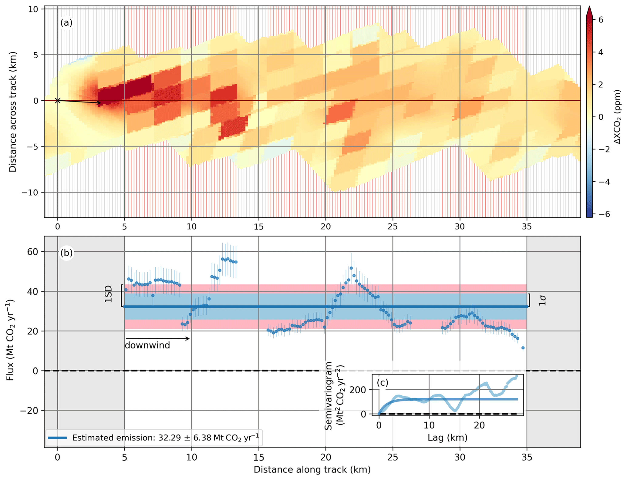
Figure 5 Example of the emission rate estimation procedure, as explained in Sect. 2.2.3, for the scene on 10 April 2020. The x axis represents the distance of the CSs from the source (at the origin) along the plume track. Panel (a) displays ΔXCO₂ within the refined plume in the track coordinate system. The black arrow shows the mean horizontal wind direction within the potential plume. The red lines denote valid CSs and the grey lines denote invalid CSs. The filled ΔXCO₂ gaps are shown together with the observations. Panel (b) shows the estimated fluxes across each valid CS along the plume track. The blue dots account for the cross-sectional fluxes used for the estimation of the mean emission rate, shown as a solid blue line. The standard deviation of the data is shown as a pink area on both sides of the mean line, and the 1σ error, calculated as described in Sect. 2.3, appears as a light-blue area. The vertical bars on each dot account for the propagation uncertainty (see Sect. 2.3.2). The fluxes through valid CSs at distances from the source outside the plume range are plotted using blue crosses. Panel (c) presents the semivariogram used to compute the dispersion uncertainty (see Sect. 2.3.1). The dots stand for the empirical semivariogram, computed using Eq. (5). The model resulting from the exponential fit (Eq. 6) is depicted using a solid line.

We accepted only the subset of CSs at distances downwind of the source larger than 5 km and smaller than 35 km. We refer to the span in between as the plume range. The lower threshold avoids errors due to both the OCO-3 product geolocation error, typically of less than 1 km and reaching up to 3 km for a fraction of the data (Payne et al., 2022), and due to the exact location of the stacks, which can be about 1 km apart. Furthermore, it accounts for the fact that the assumption of good vertical mixing of the plume within the boundary layer is realistic only after about the height of the boundary layer downwind of the source, typically in the order of 1–2 km (Matheou and Bowman, 2016). For larger distances downwind of the source, diffusion causes the dilution of the plume, reducing the XCO₂ enhancement, which can lead to the detection of only a fraction of the plume extent and, therefore, an underestimation of the computed cross-sectional fluxes. This was avoided with the upper limit of the plume range.

In addition, we filtered out CSs that are likely to yield biased estimates of the emission rate. We considered the CSs to be valid if they fulfilled all of the following conditions: (a) less than 40 % of the XCO₂ observations within the refined plume along the CS are missing, to avoid considering CSs with too many interpolated data added to fill gaps, and (b) the width of the refined plume along the CS is larger than 4 km, which ensures that the CS spans over more than one SAM footprint. After filtering out CSs outside the plume range and applying conditions (a) and (b), we are left with a subset of n^′ CSs.

With this, we computed, using Eq. (2), a set of values {f_j}, for $j=\mathrm{1},\mathrm{2},\mathrm{\dots },N$, corresponding to the CO₂ flux through each CS at distance, x_j, from the source along the plume track, where only a subset of n^′ valid CSs was considered. An example of these cross-sectional fluxes is shown as scattered blue dots along the plume track in Fig. 5b. We expect the obtained cross-sectional fluxes to vary along the track of the plume. These fluctuations partly originated from the experimental error in the quantities used in Eq. (2) but were also due to the turbulent nature of the process.

In addition, the CO₂ molecules observed in the SAM were released at different times. The farther away the CS is from the source, the longer the CO₂ molecules were released before the OCO-3 overpass time. Let us define the “plume characteristic time”, Δt, as the time that the CO₂ molecules would have needed to travel, at the mean horizontal wind speed within the potential plume, the distance between the source and the valid CS within the plume range situated the farthest away from the source. If the power plant emissions vary within this Δt, they will add another source of fluctuations to the cross-sectional fluxes. We calculated this plume characteristic time and rounded it to the nearest hour integer. For a typical plume length along its track of about 30 km, the characteristic time ranges from approximately 1 to 3 h for wind speeds between 3 and 7 m s⁻¹.

To describe the process leading to the flux fluctuations, we took a stochastic approach. Let each f_j be a realization of a random variable F(x_j) at points $x_j,j=\mathrm{1},\mathrm{2},\mathrm{\dots },N$ along the plume track. To characterize F, we assume second-order or weak stationarity (WS), which means that (a) the mean of F is constant for all x_j, which allows us to estimate the mean of the process by treating the f_j at different locations as realizations of the same random variable. This assumption is realistic as long as both the emissions from the power plant and the wind vector have no significant trend within the characteristic time interval. Furthermore, WS means that (b) the covariance, $\text{Cov}\left(F\left(x_j\right),F\left(x_{j+\mathit{\delta }}\right)\right)$, of the random variables at points x_j and x_j+δ, where $\forall \mathit{\delta }=\mathrm{0},\mathrm{1},\mathrm{2},\mathrm{\dots },N-\mathrm{1}$, depends only on the distance between two points along the plume track, $d=\left|x_{j+\mathit{\delta }}-x_j\right|$, not on their absolute positions. As all of the x_j are equally spaced, the distance between any pair of consecutive locations will be constant and given by $\mathrm{\Delta }x=x_{j+\mathrm{1}}-x_j$. Therefore, we can write the lag distance as d=δΔx, where δ is the “lag index” and, consequently, $\text{Cov}\left(F\left(x_j\right),F\left(x_{j+\mathit{\delta }}\right)\right)=C\left(\mathit{\delta }\right)$, where C is the covariance function. On account of the first assumption, we can estimate the mean emission rate, $\stackrel{\mathrm{‾}}{f}$, from the mean of the computed cross-sectional fluxes. The obtained results are detailed in Sect. 3.2 and Table 1. With the second assumption, we can also estimate its uncertainty.

2.3 Uncertainty

To estimate the uncertainty in the obtained mean emission rate, we considered three contributions:

1. The dispersion uncertainty, s_disp, includes all random effects that cause cross-sectional fluxes to oscillate about their mean. These effects have different origins, such as the inherent variability in the cross-sectional fluxes due to turbulence, variations in the emissions within the plume characteristic time or random errors in the quantities used to compute the cross-sectional fluxes.

2. The wind uncertainty, s_wind, refers to the impact on the emission rate estimate of a possible bias in the horizontal wind speed.

3. The sensitivity uncertainty, s_sens, includes the effect of different choices of the analysis parameters on the emission estimate.

Considering that all three sources of uncertainty are uncorrelated, the standard error (1σ) of the mean emission rate, $s\left(\stackrel{\mathrm{‾}}{f}\right)$, is therefore given by $s^{\mathrm{2}}\left(\stackrel{\mathrm{‾}}{f}\right)=s_{\text{disp}}^{\mathrm{2}}+s_{\text{wind}}^{\mathrm{2}}+s_{\text{sens}}^{\mathrm{2}}$. Each of the aforementioned contributions to the uncertainty is explained below, and the corresponding results are shown in Table 1.

We did not explicitly consider an XCO₂ measurement error under the assumption that, at the relatively small spatial scales of the analysed scenes, any bias in the XCO₂ data is corrected for when subtracting the background. Random errors in the XCO₂ values are included in the dispersion uncertainty.

2.3.1 Dispersion uncertainty

The dispersion uncertainty is given by the variance of the mean:

$$\begin{array}{}\text{(4)}& \begin{array}{rl}{s}_{\mathrm{disp}}^{\mathrm{2}}& =\text{Var}\left(\stackrel{\mathrm{‾}}{f}\right)={\displaystyle \frac{\mathrm{1}}{n^{\mathrm{2}}}}\sum _{j=\mathrm{1}}^n\sum _{k=\mathrm{1}}^n\text{Cov}\left(F\left(x_j\right),F\left(x_k\right)\right)\\ & \underset{\text{WS}}{=}{\displaystyle \frac{\mathrm{1}}{n}}\left(C\left(\mathrm{0}\right)+\mathrm{2}{\sum }_{\mathit{\delta }=\mathrm{1}}^{n-\mathrm{1}}\left(\mathrm{1}-{\displaystyle \frac{\mathit{\delta }}{n}}\right)C\left(\mathit{\delta }\right)\right),\end{array}\end{array}$$

where the last term is the explicit sum over the elements of the covariance matrix for a weakly stationary process divided by n² (Storch and Zwiers, 1999). Thus, we can compute the dispersion uncertainty provided that we have knowledge of the shape of the covariance function.

For uncorrelated data, C(δ)=0 for δ≥1; thus, Eq. (4) reduces to $s_{\mathrm{disp}}^{\mathrm{2}}=\frac{\mathrm{1}}{n}C\left(\mathrm{0}\right)$. However, the cross-sectional fluxes are spatially correlated, especially due to the close spacing between consecutive CSs compared with the OCO-3 spatial resolution. As the effective number of independent CSs is unknown, we performed a correlation analysis to estimate the covariance function, C(δ), which we used to estimate the dispersion uncertainty using Eq. (4).

We used a semivariogram, defined as $\mathit{\gamma }(x_j-x_k)=\frac{\mathrm{1}}{\mathrm{2}}\text{Var}\left[F\left(x_j\right)-F\left(x_k\right)\right]$, to estimate the covariance function. For a weakly stationary process, it can be written as $\mathit{\gamma }\left(\mathit{\delta }\right)=\frac{\mathrm{1}}{\mathrm{2}}\text{Var}\left[F\left(x_{j+\mathit{\delta }}\right)-F\left(x_j\right)\right]$ and fulfils that $\mathit{\gamma }\left(\mathit{\delta }\right)=C\left(\mathrm{0}\right)-C\left(\mathit{\delta }\right)$, showing, in this case, the equivalence between the semivariogram and the covariogram. When estimated from the data, the semivariogram is preferred because it does not require knowledge of the mean and is, therefore, an unbiased estimator (Montero et al., 2015). We can empirically estimate the semivariogram as follows:

$$\begin{array}{}\text{(5)}& \widehat{\mathit{\gamma }}\left(\mathit{\delta }\right)={\displaystyle \frac{\mathrm{1}}{\mathrm{2}m\left(\mathit{\delta }\right)}}\sum _{j=\mathrm{1}}^{m\left(\mathit{\delta }\right)}{\left(f_{j+\mathit{\delta }}-f_j\right)}^{\mathrm{2}},\end{array}$$

where m(δ) is the number of pairs of data, $\left\{f_{j+\mathit{\delta }},f_j\right\}$, used for the estimation. For a pair to be taken into account, both f_j+δ and f_j must correspond to valid CSs. Therefore, m decreases for larger lags, δ, and depends on the number and distribution of valid CSs.

The empirical semivariogram is only defined for a subset of the total N lags and might exhibit an erratic behaviour. A widely used solution is to use a model to fit the estimated semivariogram. A suitable model should represent some basic features, like a monotonic increase with increasing lag, which shows a decreasing correlation until the sill (horizontal asymptote) is reached, and a positive intercept that accounts for the “nugget effect”, i.e. a discontinuity at the origin (Webster and Oliver, 2007). We use an exponential model of the shape:

$$\begin{array}{}\text{(6)}& \mathit{\gamma }\left(\mathit{\delta }\right)=C\left(\mathrm{0}\right)\left(\mathrm{1}-e^{-\mathit{\delta }\mathrm{\Delta }x/l}\right),\end{array}$$

where C(0) is the variance of the process. The parameter l is a measure of the correlation length and the only free parameter to be determined by the fit. This model assumes that there is no nugget effect because we expect a smooth variation in the semivariances due to the close spacing between CSs. As the estimation of the empirical semivariances is less reliable for larger lag distances and smaller numbers of pairs, m, used for the computation, we considered only the empirical semivariances computed from a number of pairs m≥10.

With the modelled semivariogram, we computed the covariance function for each lag, δ, as $C\left(\mathit{\delta }\right)=C\left(\mathrm{0}\right)-\mathit{\gamma }\left(\mathit{\delta }\right)$, which we used to compute the dispersion uncertainty making use of Eq. (4).

The effective number of independent CSs within the plume range was estimated as follows:

$$\begin{array}{}\text{(7)}& n_{\mathrm{eff}}^{\prime }={\displaystyle \frac{C\left(\mathrm{0}\right)}{s_{\mathrm{disp}}^{\mathrm{2}}}}.\end{array}$$

For a typical plume range of 30 km and an approximate 2 km footprint width, we would expect a maximum of about 15 independent CSs. Further correlation among CSs derived from spatial structures would lead to $n_{\mathrm{eff}}^{\prime }\le \mathrm{15}$. Therefore, n^′ provides us with an intuitive check of the computed dispersion uncertainty. It is worth noting that $n_{\mathrm{eff}}^{\prime }$ is independent of the number, n^′, of valid CSs within the plume range, provided n^′ was large enough to perform the correlation analysis.

2.3.2 Wind uncertainty

The wind uncertainty, s_wind, includes the effect of a possible bias in the horizontal wind used to compute the cross-sectional fluxes on the estimated emission rate. This is a purely systematic component, as any fluctuations in the wind along the plume track are accounted for in the dispersion uncertainty.

We considered an uncertainty in the horizontal wind speed perpendicular to the CSs of $s\left(w_{⟂}\right)=\mathrm{0.5}$ m s⁻¹. This value is representative of the ERA5 ensemble spread zonal wind component close to the surface (Hersbach et al., 2020). A different approach was taken by e.g. Nassar et al. (2017), who obtained the uncertainty in the horizontal wind speed from a comparison between MERRA-2 (Modern-Era Retrospective Analysis for Research and Applications-2) and ERA5 data. However, an ensemble approach of only two methods might be insufficient to determine the wind speed uncertainty, as it would be affected by random errors from both data products.

Using Eq. (2) and substituting w_⟂ by its uncertainty, we obtain a value of the effect of the wind uncertainty on each cross-sectional flux, b_w,j. These uncertainties (b_w,j) are shown as blue bars about the flux estimates in Fig. 5b. The wind uncertainty is the mean effect of the wind bias on the emission rate estimate, i.e. the mean of b_w,j.

2.3.3 Uncertainty from sensitivity

The sensitivity uncertainty, s_sens, is a measure of the effect of different choices of the parameters used for the analysis on the emission estimate.

We estimated a measure of this uncertainty contribution from the variation in a number of parameters used for the analysis of each scene within plausible ranges:

1. the p values for the detection of the potential plume and plume refinement, in both cases ranging from 0.03 to 0.1;

2. the radius of the circle and power of the inverse distance to fill the SAM gaps within the refined plume – the radius varied from 0.05 to 0.1^∘ for inverse distance weighting and from 0.05 to 0.2^∘ for inverse squared-distance weighting;

3. the limits of the plume range, for which we varied the lower limit from 3 to 10 km and the upper limit from 30 to 40 km from the source;

4. the function used to fit the background, for which we considered three cases – linear dependence on longitude and latitude with a possible swath bias (given by Eq. 3), an analogous model also allowing for a possible footprint bias (f_k for $k=\mathrm{1},\mathrm{2},\mathrm{\dots },\mathrm{7}$), and a model considering only the linear dependence on longitude and latitude (i.e. setting $s_j=\mathrm{0}\forall j$ in Eq. 3).

For each parameter, we computed the standard deviation of the emission estimates for each scene and took its mean as a measure of the sensitivity uncertainty for that parameter. Assuming uncorrelated errors, we added them quadratically to compute an estimate of s_sens.

2.4 Sensitivity tests

In addition to the sensitivity analysis performed to obtain an uncertainty estimate, we have performed other sensitivity tests. These tests are explained in the following, and the results are presented in Sect. 3.3. The modifications evaluated in these tests have been shown to either have no significant influence on the results or lead to biased emission estimates. Therefore, we have not included the outcome of these tests in the sensitivity uncertainty. These sensitivity tests are as follows:

• a.

  In the computation of the cross-sectional fluxes, the wind speed and direction from ERA5 were used. It is common practice to rotate the wind vector to match the direction of the observed plume (e.g. Reuter et al., 2019; Nassar et al., 2017; Varon et al., 2018). Therefore, we have tested the influence of the wind rotation to match the direction of the detected plume track.

• b.

  The OCO-3 L2 XCO₂ product includes a quality flag, allowing us to filter out those observations tagged as having poorer quality. Omitting the quality filtering has the advantage of a denser coverage, and thus fewer missing SAM observations, at the expense of higher bias risk.

• c.

  We used the NO₂ VCD to obtain the shape of the potential plume, which constrains the CO₂ plume region. We tested the applicability of the method without using NO₂ measurements but constraining the CO₂ plume region by a wedge downwind of the source (as described in Sect. 2.2.1) to define the NO₂ region.

2.5 Scene selection

The analysed scenes were selected using an automatic procedure. It comprises searching for SAMs with more than 800 soundings (after quality filtering) and co-located TROPOMI NO₂ overpasses with a time difference with respect to the OCO-3 overpass that is smaller than 5 h.

We also applied additional filters in the emission quantification procedure. A scene was discarded according to the following criteria:

1. If there were less than 20 OCO-3 observations within the detected potential plume or less than 50 in the background, the scene was not included. This condition discards scenes with too few observations for our emission estimation procedure.

2. The width of TROPOMI pixels increases in the across-flight direction due to the increasing viewing angle, from about 3.6 km at nadir to about 14 km at the edges. A larger pixel size can result in an underestimation of the extent of the detected NO₂ plume with the statistical test due to the dilution of the signal; this is further intensified due to smoothing. In cases with strong NO₂ emissions, the larger pixel size can also lead to an overestimation of the detected plume, underconstraining the CO₂ plume and leading to a possible inclusion of background structures in the CO₂ plume. To avoid such cases, we omitted a scene if more than 50 % of the TROPOMI observations with an enhanced VCD belonged to the outer 50 pixels of the swath (on any side).

3. If the angle between the plume track and the wind direction was wider than 45^∘, the scene was not included. This provides an additional check on the wind direction as obtained from ERA5 and avoids the analysis of scenes in which there was an abrupt change in the wind direction shortly before the overpass.

4. If the highest computed lag distance was smaller than 2 km (about the size of an OCO-3 footprint), the scene was omitted. With this criterion, we avoid characterizing the dispersion of the fluxes along the plume track with an insufficient number of independent CSs.

2.6 Bottom-up emission estimation

To validate our top-down emission estimates, we computed the CO₂ emissions of the Bełchatów Power Station for the selected scenes at approximately the OCO-3 overpass time using a bottom-up approach based on the power plant activity.

First, an hourly bottom-up estimate of the CO₂ emissions was computed as the product of the hourly generated power and the emission intensity (mass of emitted CO₂ per unit of generated power). We used information on the hourly net generated power per generation unit of ≥100 MW installed capacity, provided by the European Network of Transmission System Operators for Electricity (ENTSO-E) on its Transparency Platform (https://transparency.entsoe.eu/, last access: 3 February 2023). The emission intensity was computed from the total CO₂ emissions divided by the net generated power by the power plant in 2018. That year, the CO₂ emissions were 38.4 Mt CO₂, as reported by the European Industrial Emissions Portal (https://industry.eea.europa.eu, last access: 20 February 2023). The European Industrial Emissions Portal collects information from the EU Registry on Industrial Sites and the European Pollutant Release and Transfer Register (E-PRTR). The net generated power in that year, according to the power plant operator (PGE, 2023), was 32.535 TW h. That yields a CO₂ intensity of $\mathrm{1.18}\times {\mathrm{10}}^{-\mathrm{6}}$ Mt CO₂ (MW h)⁻¹, which we assumed to have remained approximately constant up until 2022.

Power plant emissions have strong daily and day-to-day variations (Velazco et al., 2011). For this reason, despite providing our top-down emission estimates in units of Mt CO₂ yr⁻¹, they are not annual averages. They are up-scaled and represent the emissions within the approximate plume characteristic time, Δt, before the OCO-3 overpass. Therefore, we averaged the reported hourly generated power within that Δt before the OCO-3 overpass to compute the bottom-up emission estimates, which we can directly compare with our top-down estimates. This approach is similar to the “dynamic value” described by Nassar et al. (2021).

We estimated the uncertainty in the bottom-up emission estimates by taking two contributions into account: the “intensity uncertainty” and the “characteristic time uncertainty”. The former refers to the uncertainty in the estimated emission intensity, subject to the uncertainty in the data used in its computation. Gurney et al. (2016) analysed two emission datasets for power plants in the US, finding monthly emission differences of about 6 % for about half of the facilities. For such a large power plant, we would not expect the uncertainty to belong to the top 50th percentile. Despite that, we considered a conservative 6 % uncertainty in the CO₂ emissions from EIEP (2020), and consequently in the emission intensity computed from it. We assumed that this includes changes in the intensity over the years, the different emission intensities that the various units in the power plant have, and possible mismatches between the net generated power as reported by ENTSO-E and the power plant operator. With respect to the characteristic time uncertainty, this contribution to the uncertainty refers to the mentioned emission variations within Δt, which we account for by taking half the maximum difference in the hourly generated power times the emission intensity. The total uncertainty in our bottom-up estimates is the root sum of squares of the characteristic time and the intensity uncertainties.

Our bottom-up emission estimates are shown in Table 1, along with their corresponding uncertainties.

3 Results

3.1 Scene selection

In the period from the beginning of the OCO-3 XCO₂ dataset in July 2019 until November 2022 inclusive, we found a total of 94 SAMs over the Bełchatów Power Plant, 14 of which have more than 800 soundings (after quality filtering). All 14 of these SAMs have at least one co-located S5P overpass with a time difference smaller than 5 h. After applying the scene selection filters mentioned in Sect. 2.5, we were left with nine scenes, corresponding to nine different SAMs.

3.2 CO₂ emission estimates

The results for these nine scenes obtained from the scene selection are detailed below, illustrated in Fig. 9 and summarized in Table 1 (along with the meteorological information for each scene and several other parameters that characterize the scene). The correlation between our top-down (TD) and bottom-up (BU) estimates is 0.92, and the results obtained using these two methods agree in eight out of nine cases within their 1σ uncertainty range. Their mean difference (TD − BU) is −2.8 Mt CO₂ yr⁻¹ and their standard deviation is 3.7 Mt CO₂ yr⁻¹. The mean uncertainty for these nine scenes is 5.8 Mt CO₂ yr⁻¹ (22.0 %), and it is dominated by the dispersion uncertainty, which is on average about 1.8 times higher than the wind uncertainty and slightly larger (on average 1.3 times higher) than the sensitivity uncertainty.

The results obtained for the nine analysed scenes are detailed below. They are illustrated in Figs. 3–8 for some of the overpasses and in Figs. A1–A5 in Appendix A for those overpasses not shown in this text. We refer to overpass times in local time (LT), as determined by the corresponding time zone. All of the overpass times for the analysed scenes for the Bełchatów power station refer to Central European Summer Time (CEST). The results for each scene are as follows:

10 April 2020

The OCO-3 overpass began at 15:35 LT (CEST), while the co-located S5P overpass began at 12:57 LT. Our TD CO₂ emissions are estimated to be 32.29±6.38 Mt CO₂ yr⁻¹. The mean horizontal wind speed within the potential plume was 3.39 m s⁻¹ with an angle relative to the plume track of about −4.7^∘. The characteristic time was estimated to be about 3 h. Within that characteristic time before the OCO-3 overpass, all of the units were operative and the BU estimated emissions decreased by 3.51 Mt CO₂ yr⁻¹. Within that time, there was a gradual 1.5 m s⁻¹ increase in the wind speed and an angle shift of 13.94^∘ about the plume track. The steps to compute the emission estimate and the results are shown in Figs. 3–5.

17 April 2020

The OCO-3 overpass was at 11:42 LT, while the S5P overpass began at 14:06 LT. Our TD emission estimate is 32.04±10.27 Mt CO₂ yr⁻¹, as illustrated in Fig. 6. The averaged wind speed within the potential plume at the OCO-3 overpass time was 5.86 m s⁻¹, with an angle of 18.4^∘ with respect to the detected plume track. We estimated a characteristic time of approximately 2 h. Within that characteristic time before the OCO-3 overpass, the wind speed slightly increased to then decreased by a total amount of about 0.79 m s⁻¹, while its angle remained approximately constant. We refer to an approximately constant wind speed or wind direction if its change within the characteristic time is less than 0.5 m s⁻¹ or 10^∘, respectively. The power plant activity slightly decreased within the characteristic time, from 3381 to 3041 MW h, leading to a BU age uncertainty of 1.63 Mt CO₂ yr⁻¹. The dispersion uncertainty of 9.28 Mt CO₂ yr⁻¹ is the largest among all of the analysed scenes. In Fig. 6c and d, we can appreciate the oscillations in the cross-sectional fluxes, with a CO₂ accumulation at higher distances from the source.

18 June 2021

Figure 7 shows the results for this overpass. The TD emission estimate is 32.77±5.40 Mt CO₂ yr⁻¹. Within the 2 h characteristic time prior to the overpass, the wind speed increased by 0.71 m s⁻¹, while the wind direction remained approximately constant. The generated power also remained approximately constant, as shown by the relatively small age uncertainty (0.12 Mt CO₂ yr⁻¹).

19 June 2021

The potential plume extends, in this case, to areas without OCO-3 observations. Therefore, we have obtained cross-sectional fluxes only up to a distance from the source of about 23 km. Our TD emission estimate is 41.94±6.99 Mt CO₂ yr⁻¹. The results for this overpass are shown in Fig. A1.

20 June 2021

The low power plant activity (operating at less than 40 % of its maximum capacity) and the relatively high wind speed of 6.80 m s⁻¹ resulted in enhancements over the background of the same order of magnitude as the background structures; thus, the emission plume is hardly perceptible at first sight (see Fig. A2). The estimated TD emissions are 17.96±3.83 Mt CO₂ yr⁻¹. Within the 1 h (characteristic time) prior to the OCO-3 overpass, the wind speed decreased by about 0.61 m s⁻¹, while the wind direction and the power-plant-generated power remained approximately constant. The large fraction of missing OCO-3 observations within the refined plume led to the omission of about two-thirds of the defined CSs within the plume range, especially at distances of between 14 and 23 km from the source. The low number of valid CSs, distributed in blocks spanning over less than 5 km and with gaps reaching 10 km, led to a likely incomplete characterization of the correlation of the cross-sectional fluxes and, thus, to an underestimation of the dispersion uncertainty (1.88 Mt CO₂ yr⁻¹). The inference of an underestimated dispersion uncertainty can also be reached when looking at the unexpectedly high computed effective number of independent CSs.

8 October 2021

The large fraction of missing (quality-filtered) SAM observations led to the near absence of valid CSs to compute the fluxes for distances less than about 23 km downwind of the source. We observed (Fig. A3) a near-monotonic increase in the fluxes with distance downwind of the source over about 10 km. This increase could be attributed, at the first instance, to a violation of the stationarity assumption that we made to estimate the mean emission rate and its uncertainty. However, the change in the generated power within the characteristic time is in the order of 10 %, while the fluctuations in the cross-sectional fluxes are at least 1 order of magnitude larger. The wind speed and the power plant activity remained approximately constant within the characteristic time of 1 h before the overpass. Therefore, a plausible cause of the apparent monotonic change in the cross-sectional fluxes is the turbulent flow, where we missed part of the oscillating behaviour due to the cut-off of 35 km along the plume track. This explanation seems consistent with Fig. A3d, where we observe a decrease in the cross-sectional fluxes at distances greater than 35 km downwind.

9 October 2021

The results for the 9 October 2021 scene are shown in Fig. 8. The wind speed and power generation are comparable to those determined for the scene on 20 June 2021. The relatively large fraction of gaps within the potential plume and the low enhanced ΔXCO₂ led to an apparent underestimation of the refined plume extent before about 18 km downwind of the source. This is the only case where the obtained TD estimate (11.59±4.12 Mt CO₂ yr⁻¹) does not agree with our BU estimate (19.54±1.48 Mt CO₂ yr⁻¹) within the uncertainty ranges.

24 June 2022

The OCO-3 overpass took place at 09:01 LT and is the earliest of all of the scenes investigated. Despite the 4 h time difference with the TROPOMI overpass, which is the largest of the analysed scenes, the detected potential plume seems to well-constrain the OCO-3 plume (see Fig. A4). The wind was highly variable during this scene. In the characteristic time of 1 h before the OCO-3 overpass, the wind speed increased by 3.73 m s⁻¹ and its direction changed by 13.35^∘.

13 October 2022

The TD emission estimate is 27.75±6.08 Mt CO₂ yr⁻¹. Within the 1 h characteristic time before the overpass, the wind speed and direction remained constant, and there was a drop in the generated power, from 3045 to 2464 MW, resulting in a higher age uncertainty than for other scenes, although it was smaller than the dispersion uncertainty. This overpass is illustrated in Fig. A5.

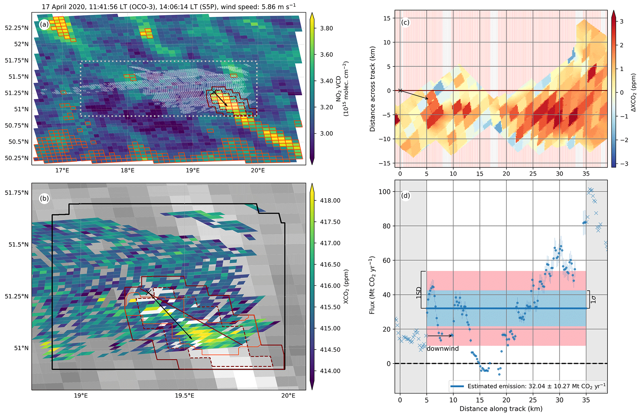
Figure 6 Overview of the top-down emission rate estimation steps for the scene on 17 April 2020. Panel (a) displays the NO₂ VCD. The SAM footprints are enclosed by grey polygons. As in Fig. 3, the observations with enhanced ΔVCD, as obtained from the t test, are enclosed by orange polygons. The SAM region is depicted using a dashed grey line. The dashed red line surrounds the cluster closest to the source and the solid red line accounts for the potential plume. Panel (b) shows XCO₂ over NO₂ VDC in the background (greyscale). The solid black line encloses the XCO₂ background area (excluding the potential plume). The refined plume is enclosed by the solid orange line within the potential plume. The straight line that traverses the potential plume is the computed track. Panel (c) is analogous to Fig. 5a. Panel (d) is analogous to Fig. 5b. The black arrows in panels (a)–(c) depict the mean horizontal wind within the potential plume. The black cross represents the source location.

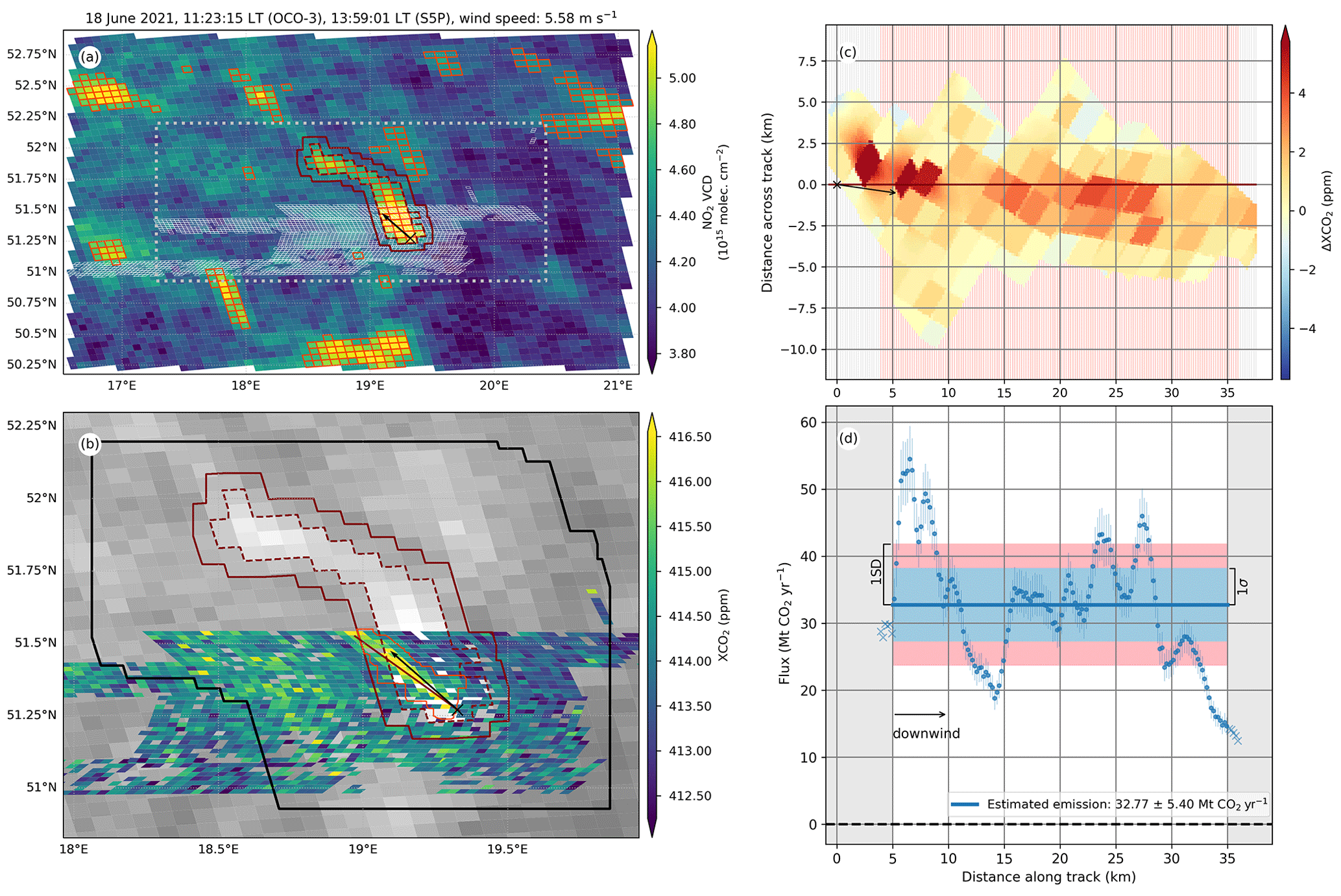
Figure 7 Overview of the top-down emission rate estimation steps for the scene on 18 June 2021. The panels are analogous to those in Fig. 6.

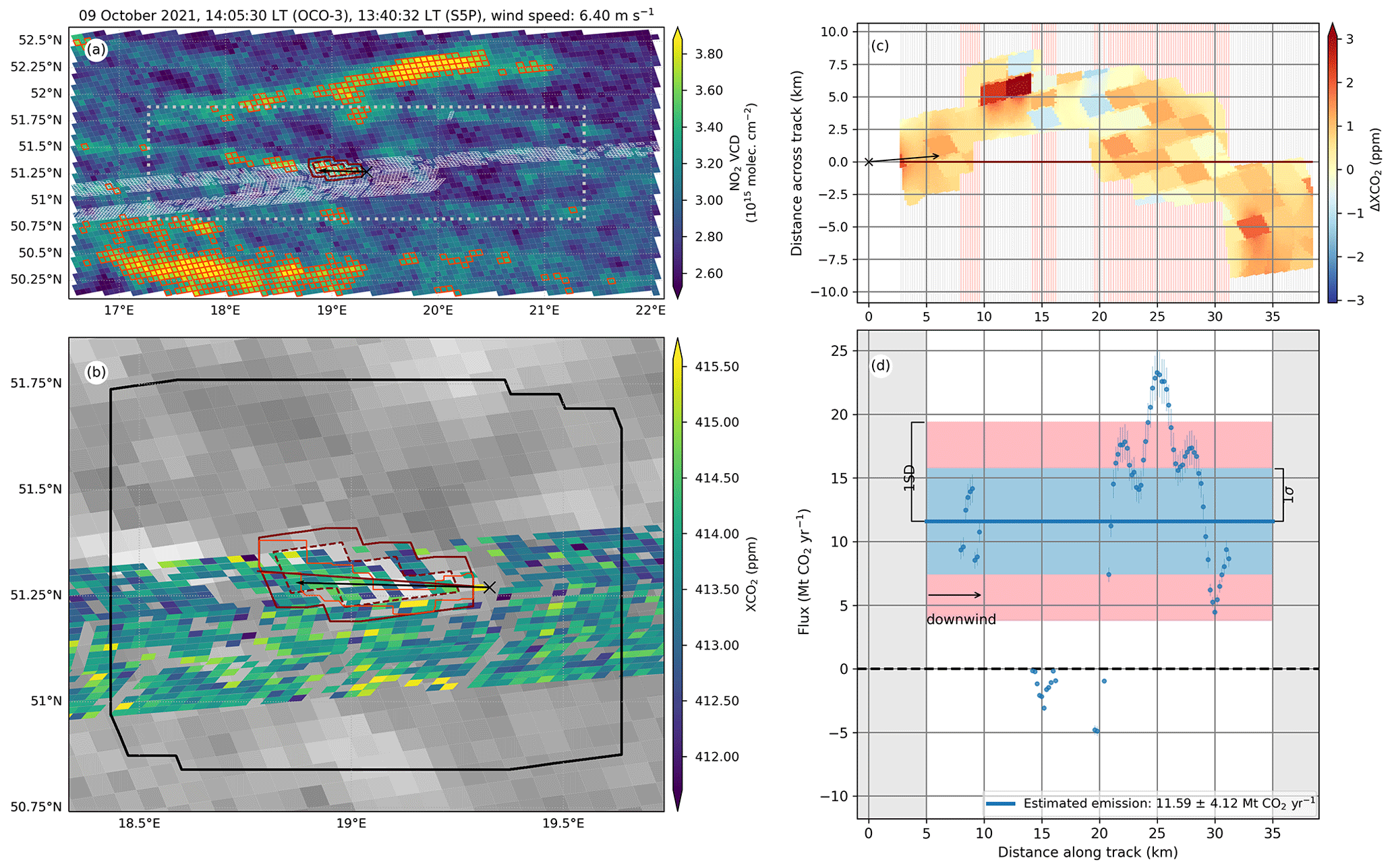
Figure 8 Overview of the top-down emission rate estimation steps for the scene on 9 October 2021. The panels are analogous to those in Fig. 6.

(Nassar et al., 2022)(Nassar et al., 2022)(Nassar et al., 2022)(Nassar et al., 2022)

Table 1 Parameters characterizing each of the analysed scenes including CO₂ emission estimates. The satellite overpass times (local time) and the meteorological information at the OCO-3 overpass time are shown. The angle refers to that between the wind vector and the north-to-south direction, positive in the clockwise direction. The top-down and bottom-up emission estimates are shown along with their corresponding uncertainties, broken down into their components as described in Sect. 2.3. The sensitivity uncertainty of 3.11 Mt CO₂ yr⁻¹ is included in the total top-down uncertainty estimates.

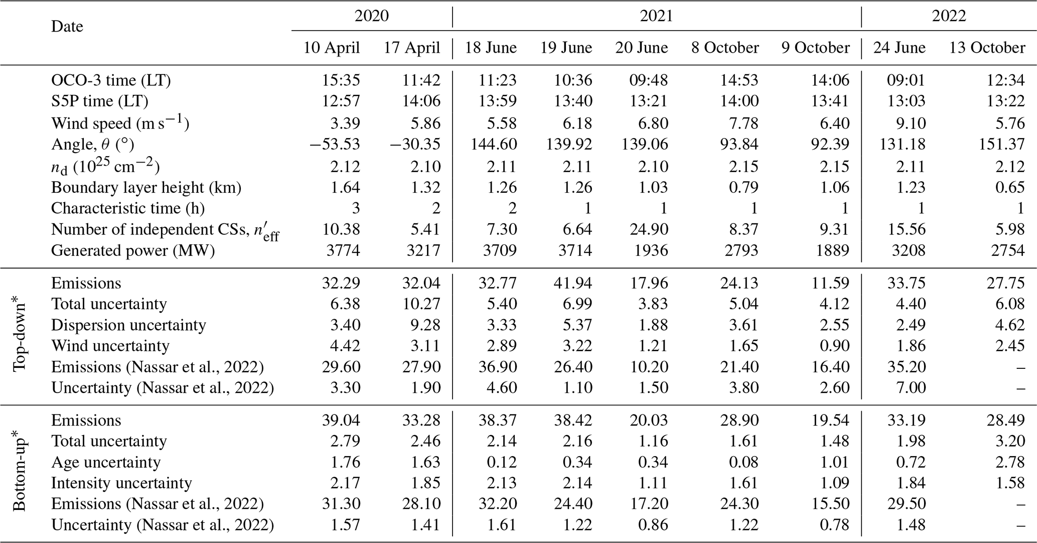
^* All quantities expressed in Mt CO₂ yr⁻¹.

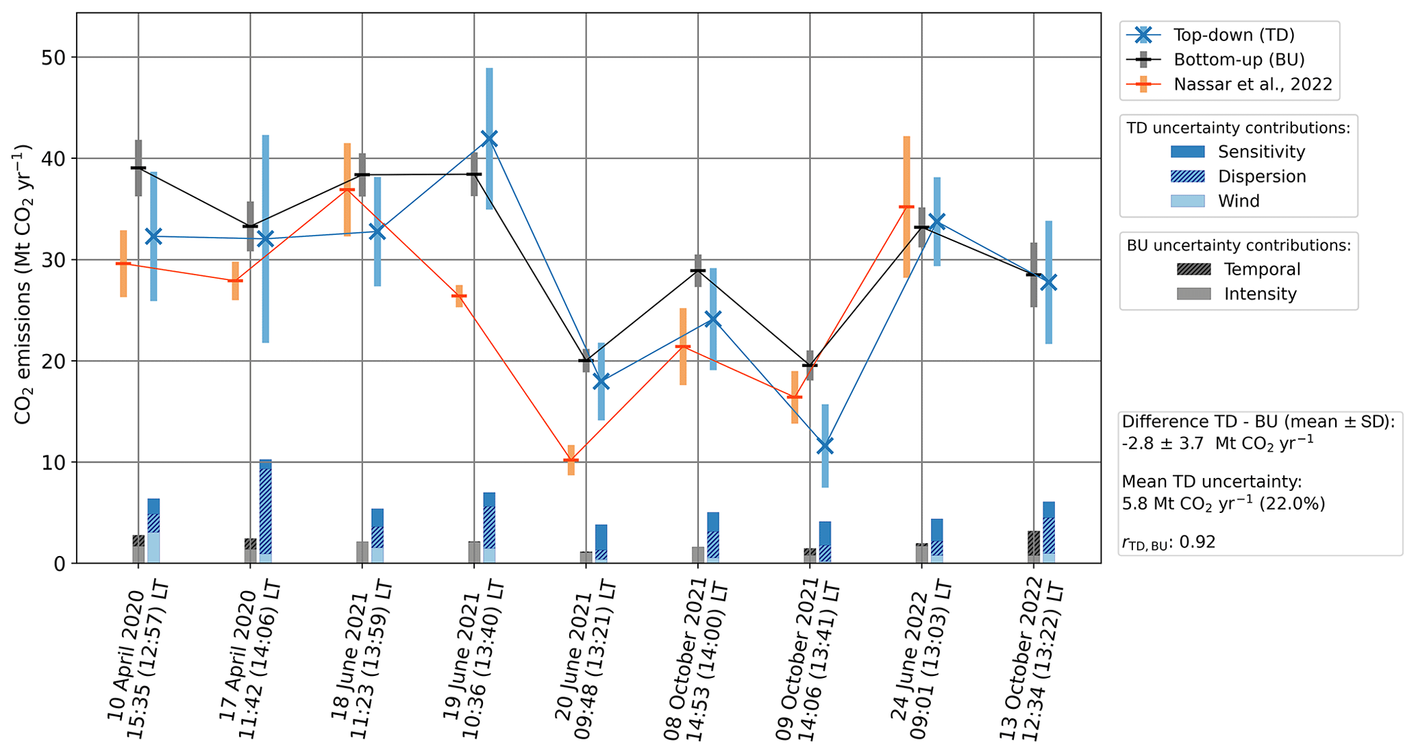
Figure 9 Bottom-up (black), top-down (blue) and Nassar et al. (2022) (orange) emission estimates for the analysed scenes. The 1σ uncertainties are displayed as bars about the corresponding emission estimate. The same uncertainties are shown at the bottom, revealing the relative contributions to the bottom-up and top-down emission estimates, where the bar's length is the respective uncertainty contribution quadratically scaled with respect to the total uncertainty.

3.3 Sensitivity analysis

As a result of the sensitivity analysis explained in Sect. 2.3.3, we obtained a measure of the sensitivity uncertainty, which is included in the total uncertainties in our TD estimates. We obtained sensitivity uncertainties of (1) 1.24 and 1.36 Mt CO₂ yr⁻¹ for the p-value sensitivity for the potential plume detection and plume refinement, respectively; (2) 0.74 Mt CO₂ yr⁻¹ for the filling parameter sensitivity; (3) 0.70 and 1.24 Mt CO₂ yr⁻¹ for the lower and upper limit of the plume range, respectively; and (4) 1.94 Mt CO₂ yr⁻¹ for the background model. Assuming uncorrelated uncertainty contributions, this results in a total s_sens of 3.11 Mt CO₂ yr⁻¹.

In the sensitivity tests (a)–(c), described in Sect. 2.4, we analysed (a) wind rotation to match the detected plume track, (b) omission of quality filtering of XCO₂ data and (c) omission of the use of NO₂ data to detect the potential plume. The results that we obtained for these tests are shown in Fig. A7 in Appendix A and summarized in the following:

• a.

  When automatically rotating the wind direction to match that of the detected plume track, we did not observe significant differences in the obtained emission rates (see Fig. A7a) because the angle that the mean wind speed forms with the detected plume track was, for the analysed scenes, between 1.4 and 18.4^∘. The absolute mean difference between BU and TD estimations slightly decreased (from −2.8 to −2.4 Mt CO₂ yr⁻¹) and its standard deviation increased by 0.3 Mt CO₂ yr⁻¹.

• b.

  A larger disparity was found when switching off the quality filtering in the XCO₂ data. In this case, as summarized in Fig. A7b, we found that running the same analysis including the XCO₂ observations considered to have a poor quality results in a correlation coefficient of about 0.45 and a standard deviation of the difference (BU − TD) of 14.7 Mt CO₂ yr⁻¹. This discrepancy was especially remarkable in the scenes where the emission plume is close to the lignite pit, situated just a few kilometres south-west of the Bełchatów power plant, where a region of elevated ΔXCO₂ is noticeable in most of the SAMs. In these scenes, the observations with elevated ΔXCO₂ were masked as belonging to the plume. If we discard the scenes in which the wind blows towards the pit region (about 90^∘), i.e. the scenes on 8 and 9 October 2021, we obtain a correlation coefficient of 0.86 and the difference (TD − BU) becomes $-\mathrm{3.50}\pm \mathrm{5.91}$ Mt CO₂ yr⁻¹. Two additional scenes passed our scene selection filters in this case – 27 June and 10 October 2022.

• c.

  Omitting the use of NO₂ data to detect the potential plume also led to a noticeable decrease in the correlation coefficient (to 0.26) and a TD − BU difference of $-\mathrm{2.2}\pm \mathrm{10.1}$ Mt CO₂ yr⁻¹, as we can see in Fig. A7c. The main reason for the decreased correlation is the larger potential plume, which underconstrained the CO₂ plume region, thereby resulting in the inclusion of neighbouring background structures of enhanced ΔXCO₂ in the detected plume, e.g. on the SAMs on 18 June 2021 (shown in Fig. A8) and 24 June 2022. In addition, no CO₂ plume was detected for the SAM on 20 June 2021 using the same p value employed for the NO₂ data. A higher p value leads to the detection of the CO₂ plume in this case, although it can also result in the further inclusion of background structures in the detected plume. A higher sensitivity (2.77 Mt CO₂ yr⁻¹) to the chosen p value was found.

4 Discussion and conclusions

With our data-driven cross-sectional flux method using co-located CO₂ and NO₂ satellite data, we were able to quantify the CO₂ emissions from the Bełchatów Power Station. We estimated the power plant CO₂ emissions for nine automatically identified different OCO-3 overpasses and compared the results with bottom-up (BU) emission estimates, finding a good correlation (0.92). The results obtained using these two methods agree in eight out of nine analysed cases within their uncertainty range.

Nassar et al. (2022) also analysed eight of our nine scenes. Their results are shown in Fig. 9 and Table 1 along with our results. We analysed an additional scene on 13 October 2022, not shown by Nassar et al. (2022). Conversely, Nassar et al. (2022) showed a SAM corresponding to 27 June 2022 that was discarded by our filtering algorithm (Sect. 2.5) due to the lack of plume observations left after dumping the OCO-3 retrievals flagged as being of poor quality. Our top-down (TD) estimates agree with those obtained from Nassar et al. (2022) in six out of eight cases. The emission estimates of Nassar et al. (2022) (NA) have a correlation coefficient of 0.85 with our BU estimates, and the NA − BU difference (mean ± standard deviation) is $-\mathrm{5.8}\pm \mathrm{4.8}$ Mt CO₂ yr⁻¹. The correlation coefficient between NA and TD is 0.76, with a mean NA − TD difference (mean ± standard deviation) of $-\mathrm{2.8}\pm \mathrm{6.7}$ Mt CO₂ yr⁻¹. Nassar et al. (2022) also computed BU emission estimates based on the generated power by the power plant. However, their BU estimates are scaled by their mean TD emission estimates. Therefore, we have not performed any comparisons with the BU estimates of Nassar et al. (2022).

The relative uncertainties for individual overpasses lie between 13 % and 32 % (22.0 % on average), higher than those of 3.8 %–19.7 % (12.2 % on average) obtained by Nassar et al. (2022). The obtained relative uncertainties are of the same order of magnitude as the uncertainty levels to be achieved with the CarbonSat mission (Buchwitz et al., 2013; Bovensmann et al., 2010), which aimed for about 20 % uncertainty in the CO₂ emission estimate for individual overpasses (ESA, 2015). The dispersion uncertainty dominates over that of wind and sensitivity, as it accounts for the large fluctuations in the cross-sectional fluxes. Using simulated plumes, Brunner et al. (2023) showed that estimated individual (2 km wide) cross-sectional fluxes fluctuate about 20 %–30 % due to turbulence, even with perfect knowledge of the ΔXCO₂ map and wind speed. A similar outcome was obtained by Wolff et al. (2021). We have observed more pronounced fluctuations, with standard deviations ranging from 27 % to 67 % of the corresponding mean emission estimate. We expect these larger fluctuations to arise from the use of modelled data in the mentioned studies, as opposed to our measurement-based analysis. Despite the large fluctuations in individual cross-sectional fluxes, having multiple CSs downwind of the source enabled their correlation to be investigated, which led to dispersion uncertainties between about 1.88 and 9.28 Mt CO₂ yr⁻¹. To obtain a qualitative check on the obtained dispersion uncertainties, we computed the effective number of CSs for each scene using Eq. (7), as shown in Table 1. In agreement with the reasoning made in Sect. 2.3.1, we obtained typical effective numbers of about 15 CSs or less. A noticeable exception is the unexpectedly high effective number of CSs (24.90) obtained for the scene on 20 June 2021 (Fig. A2). This is probably a consequence of the low number of valid CSs, distributed in blocks of about 5 km or less, with gaps between the blocks reaching 10 km, which likely led to an incomplete characterization of the correlation of the cross-sectional fluxes and, in this case, to an underestimation of the dispersion uncertainty.

The sensitivity uncertainty (3.11 Mt CO₂ yr⁻¹) shows fair stability of the method over the used parameters. All of the contributions to the sensitivity uncertainty that are accounted for are of the same order of magnitude. The choice of the p value was of little influence for most of the analysed scenes, for both the plume detection and the refinement, as long as it was large enough to detect the full extent of the actual emission plume and there were no other structures with elevated ΔXCO₂ close to the plume. The choice of the p value only had a significant effect (about 5–6 Mt CO₂ yr⁻¹) for plume detection in the 20 June 2021 scene (Fig. A2), due to the structures with elevated ΔXCO₂ in the vicinity of the plume, included within the potential and refined plume for higher p values. We encountered a similar situation when setting the upper limit of the plume range along its track, with very small fluctuations for every scene except that on 17 April 2020 (Fig. 6), for which the estimated emission rate increased about 10 Mt CO₂ yr⁻¹ when varying the parameter from 30 to 40 km. This results from an accumulation of CO₂ at those distances along the plume track.

In some of the analysed scenes there seemed to be deviations from our assumption of stationarity. For example, we observed significant wind speed variability within the characteristic time for the overpass on 24 June 2022 and less-notable variability on 10 April 2020, 17 April 2020 and 18 June 2021. We also observed noticeable changes in the power-plant-generated power, as occurred on 13 October 2022. These deviations are partly considered in the dispersion uncertainty because they can enhance or reduce the fluctuations and be partly masked by them. For example, a monotonic decrease in the wind speed would lead to an underestimation of the cross-sectional fluxes that becomes more pronounced with distance from the source. For a relatively large decrease of 1 m s⁻¹ in the wind speed, from a typical wind speed of about 6 m s⁻¹ and emissions of 30 Mt CO₂ yr⁻¹, variations of less than about 5 Mt CO₂ yr⁻¹ would be expected for individual CSs, which are much smaller values than the oscillations observed in the cross-sectional fluxes.

We have identified no significant difference between considering the wind direction obtained from ERA5 and rotating it to match the detected plume track. For this reason, we have used the ERA5 wind speed, as this has the advantage of being able to account for variable wind directions along the plume track. In addition, it is independent of any assumption regarding the shape of the plume track (in our case linear) and any possible difference between our detected plume track and the plume centreline. An advantage of the wind rotation would be a potential increase in the number of analysed scenes, as we have discarded scenes with an angle larger than 45^∘ between the detected track and the mean wind direction (see Sect. 2.5). However, such a large difference between the detected track and the mean wind direction may indicate a bias in the wind vector; therefore, discarding that scene is the most prudent option.

We have observed significant disagreement between BU and TD estimates when using the XCO₂ observations flagged as having poor quality. Nevertheless, after discarding the scenes in which the emission plume was close to the lignite pit, the disagreement between performing or non-performing quality filtering was significantly smaller. The better agreement between TD and BU estimates when disregarding these scenes suggests the presence of possible artefacts in the XCO₂ estimates over the pit regions as well as the importance (for the application of our method) of accurate XCO₂ measurements and reliable quality filtering in the case of potential biases in the XCO₂. However, an analysis with more scenes is needed for a more conclusive result. A larger number of scenes were successfully analysed using our method, at the cost of a reduced correlation between BU and TD estimates.

The TD − BU difference had a large standard deviation when the potential plume was not detected using NO₂ data but rather through a wedge centred on the mean wind vector. This disagreement appears to result from the inclusion of background structures with enhanced ΔXCO₂ (of about the same order of magnitude as the ΔXCO₂ resulting from the power plant emissions) close to the source in the detected plume. The reason for this is that the potential plume defined through this wedge downwind has a greater extent than that detected using NO₂; therefore, it constrains less of the region for CO₂ plume detection. Some examples of this inclusion of background structures in the refined plume happened for the overpasses on 18 June 2021 (shown in Fig. A8) and 24 June 2022. In these cases, the discrimination between background features and signal due to the source emissions is difficult without ancillary data. In addition, no CO₂ plume was detected for the SAM on 20 June 2021 without the aid of NO₂ data. With this, we confirmed the usefulness of NO₂ data to constrain the CO₂ plume region. These data helped us define a CO₂ background region and exclude false positives, i.e. pixels wrongly assigned as belonging to the plume.

The presented method has some limitations. It can only quantify CO₂ emissions from isolated sources. The use of NO₂ allows us to identify scenes and targets whose emission plumes might be affected by other emission sources, but no decoupling has been attempted. In addition, the method relies on the confinement of the CO₂ plume to the detected potential plume. In general, we found good agreement. However, we might encounter cases, such as the scene on 18 June 2021 (Fig. 7), in which the CO₂ plume seems to extend beyond the potential plume boundaries. In the aforementioned case, the part of the CO₂ plume that we miss is mostly beyond the plume range, having only a small effect on the final result, but it could lead to a significant underestimation of the emissions in other cases. This mismatch is due to a change in the wind direction in the time between the OCO-3 and S5P overpasses and will be solved with the use of simultaneously retrieved XCO₂ and NO₂ maps (at the same spatial resolution) from the future CO2M, from which we expect to detect potential plumes with a higher congruity with the CO₂ one.

Furthermore, we have focused on one of the power plants with the highest emissions in the world. We have obtained successful TD estimates for individual overpasses with estimated BU emissions as low as about 19–20 Mt CO₂ yr⁻¹. This suggests the feasibility of tracking power plants whose emissions are of about that magnitude. Power plants emitting over 20 Mt CO₂ yr⁻¹ are responsible for roughly 5 % of the total annual power plant CO₂ emissions (Strandgren et al., 2020). The uncertainty in the presented method is expected to scale with the source emissions. The dispersion uncertainty includes terms that are expected to be proportional to the emissions, e.g. those resulting from turbulence effects, as well as other terms that are independent of the emissions, such as those derived from XCO₂ random error. The sensitivity uncertainty also has terms proportional to the emissions, resulting from factors such as the uncertainty derived from the gap-filling method, and terms that are independent of the emissions, such as those resulting from the uncertainty derived from the function used to fit the XCO₂ background. The wind uncertainty is proportional to ΔXCO₂; thus, we can assume that this component of the total uncertainty will also be directly proportional to the emissions. Therefore, we would expect uncertainties with a similar proportionality factor to that obtained in the present study (22 % of the emission rate) for power plants whose emissions are comparable to those of Bełchatów. For power plants with lower CO₂ emissions, the absolute total uncertainty is expected to decrease accordingly, with a lower threshold determined by the terms independent of the emissions. These terms will presumably lead to a higher relative uncertainty for power plants with lower CO₂ emissions.

With our cross-sectional flux method, we have shown the potential to monitor CO₂ emissions from individual power plants by employing OCO-3 XCO₂ observations. Using such a method, we can obtain independent emission estimates, which are crucial for facilities with limited or missing information on activity data. The TROPOMI NO₂ column densities have proven useful to detect the emission plume in scenes with other neighbouring sources or small-scale background structures with enhanced XCO₂. The application of our method to observations from the planned CO2M is expected to have many advantages. The simultaneous CO2M measurements of NO₂ and XCO₂ at the same spatial resolution, which is similar to that of OCO-3, will increase the spatial correlation between NO₂ and XCO₂ images, and thus allow us to constrain the CO₂ plume better, which will lead to an increase in the accuracy of the emission estimates as well as reduced uncertainty.

Appendix A: Additional figures

In Sect. 3 of the main text of this paper, we described each of the analysed scenes and detail the results obtained for each of them. Some of these scenes are also displayed in Figs. 3–8. Figures A1–A5 illustrate the obtained results for the scenes mentioned in Sect. 3 but not shown there.

The sensitivity analysis performed to obtain the uncertainty from sensitivity is described in Sect. 2.3.3. The obtained results are shown in Sect. 3.3 and also illustrated in Fig. A6, which shows the sensitivity analysis with respect to the considered parameters, as described in Sect. 2.3.3.

The semivariograms used to compute the dispersion uncertainty according to Sect. 2.3.1 are shown in Fig. A9.

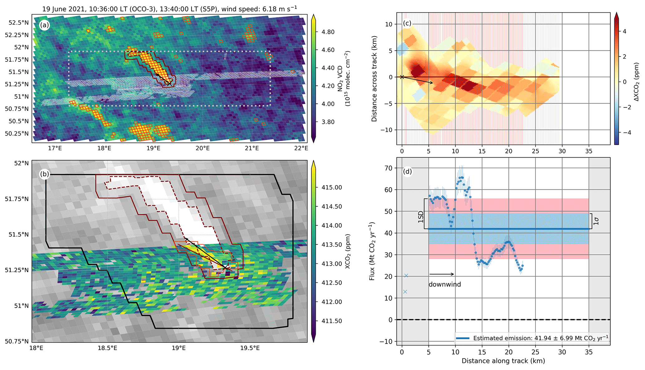
Figure A1 Overview of the top-down emission rate estimation steps for the scene on 19 June 2021. The panels are analogous to those in Fig. 6 in the main text.

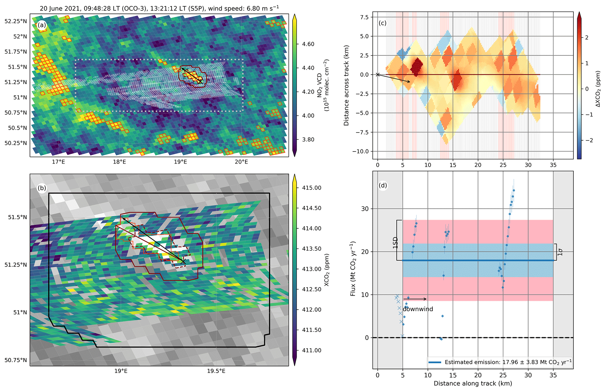
Figure A2 Overview of the top-down emission rate estimation steps for the scene on 20 June 2021. The panels are analogous to those in Fig. 6 in the main text.

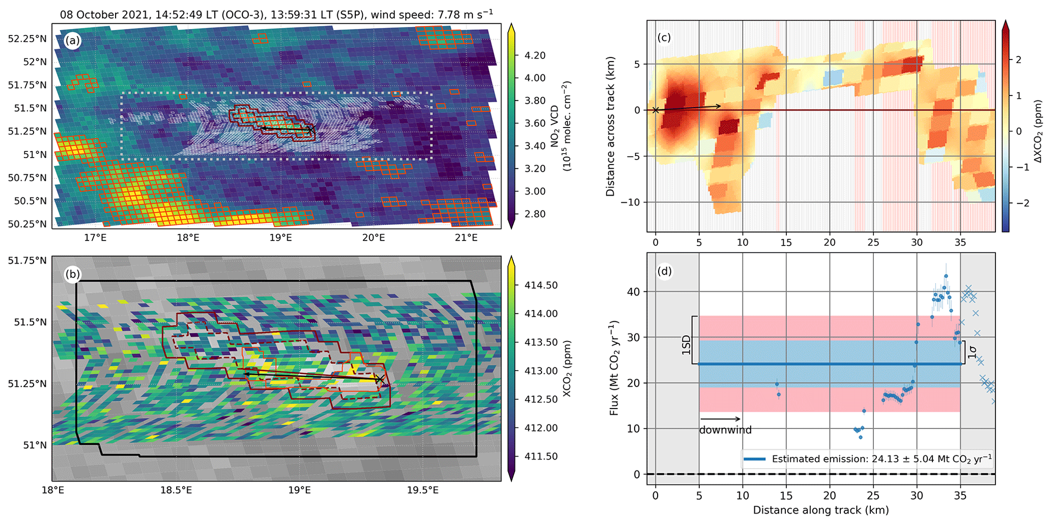
Figure A3 Overview of the top-down emission rate estimation steps for the scene on 8 October 2021. The panels are analogous to those in Fig. 6 in the main text.

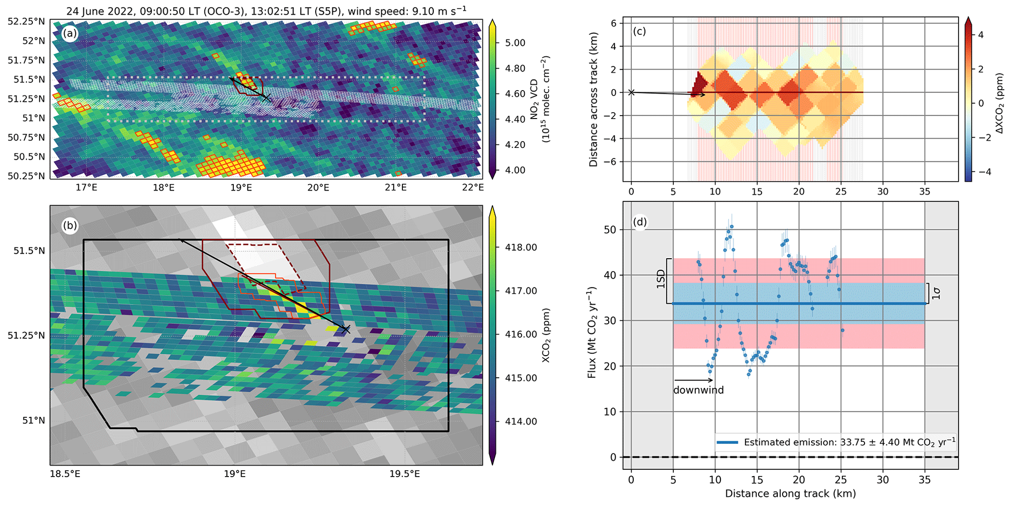
Figure A4 Overview of the top-down emission rate estimation steps for the scene on 24 June 2022. The panels are analogous to those in Fig. 6 in the main text.

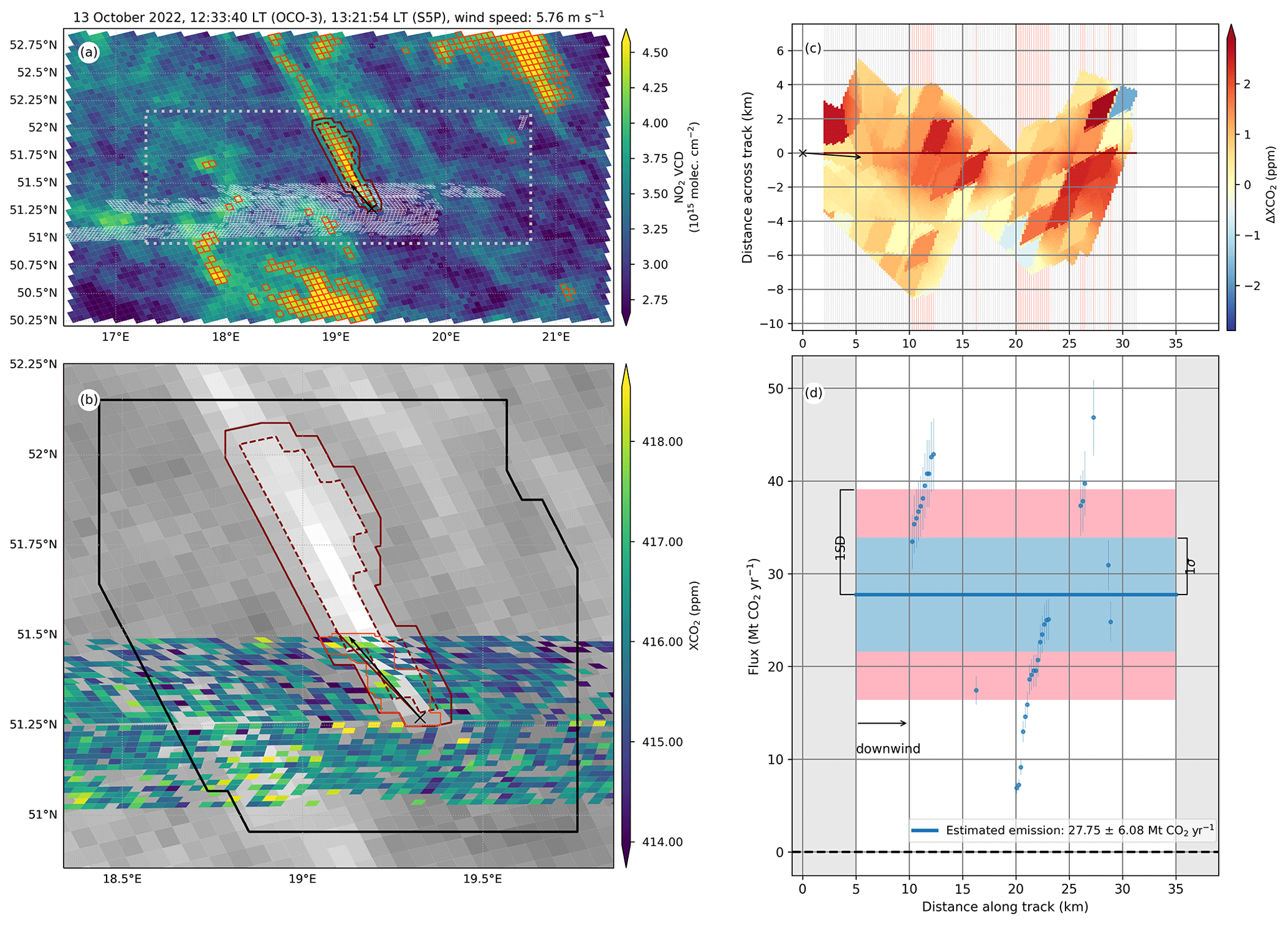
Figure A5 Overview of the top-down emission rate estimation steps for the scene on 13 October 2022. The panels are analogous to those in Fig. 6 in the main text.

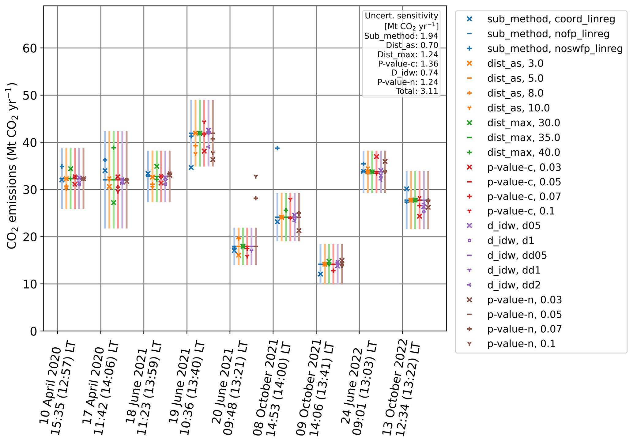
Figure A6 Sensitivity analysis performed to estimate a measure of the sensitivity uncertainty. The legend shows the names of the parameters taken into account and the values considered in each case. The p values for the detection of the potential plume (p-value-n) and for plume refinement (p-value-c) are calculated by taking values from 0.03 to 0.1 in both cases. The area and weighting of the distance weighting interpolation (d_idw) are shown, where “d” indicates inverse distance weighting interpolation, “dd” indicates the squared inverse distance weighting interpolation and the numbers refer to the radius of the used area (in tenths of degrees). The limits of the plume range (dist_as and dist_max for the lower and upper thresholds, respectively) are also shown; the values are in kilometres. The functions used to fit the XCO₂ background (sub_method) are given: linear dependence on longitude and latitude with a possible swath bias (nofp_linreg), linear dependence on longitude and latitude with a possible swath and footprint biases (coord_linreg), and only linear dependence on longitude and latitude (noswfp_linreg). Each data point stands for the result of the analysis using the value indicated by the marker for each considered parameter. The dashes stand for the values used for the main analysis. The bars show, for each scene, the total uncertainty obtained using the parameters selected for the main analysis.

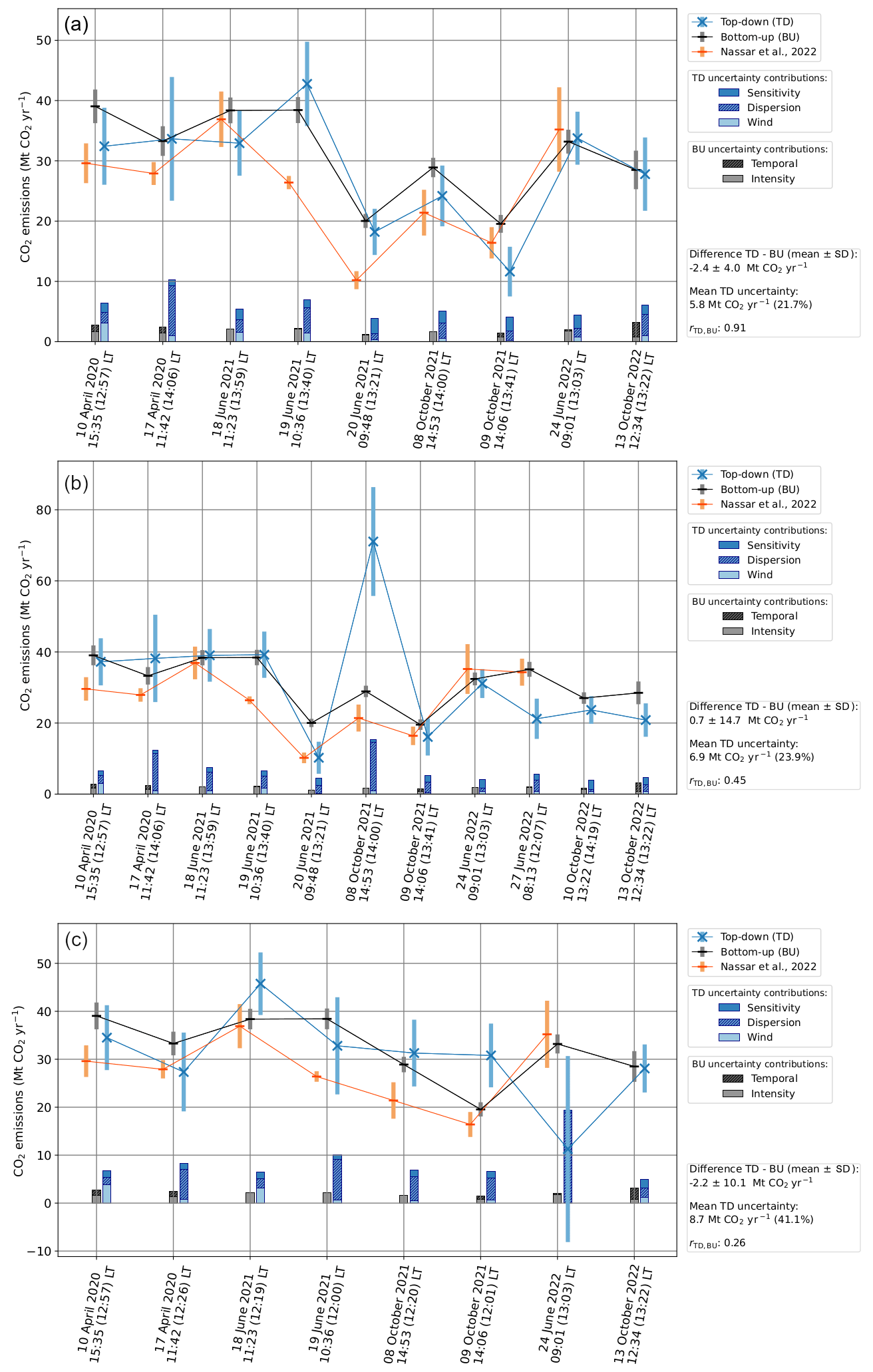
Figure A7 Summary of the results, analogous to Fig. 9, for the sensitivity tests: (a) rotation of the wind direction to match the plume track, (b) no quality filtering of the XCO₂ data and (c) potential plume definition through a wedge downwind of the source instead of NO₂ VCD.

Figure A8 Overview of the top-down emission rate estimation steps for the scene on 18 June 2022. The panels are analogous to those in Fig. 6 in the main tex. Instead of NO₂ data, a wedge downwind of the source was used to define the potential plume NO₂ (as described in Sect. 2.4).

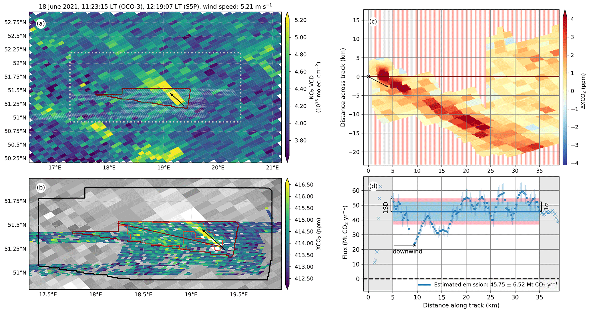
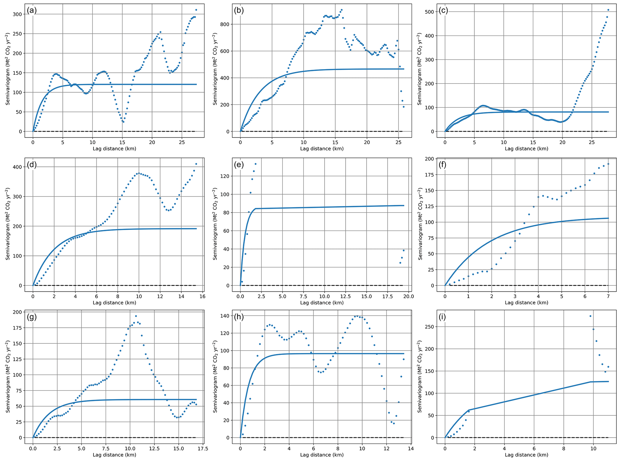
Figure A9 Semivariograms used to compute the dispersion uncertainty (see Sect. 2.3.1), analogous to Fig. 5c, for each of the nine analysed scenes. The blue dots stand for the empirical semivariogram, computed using Eq. (5). The exponential fit according to Eq. (6) is shown as a solid line for (a) 10 April 2020, (b) 17 April 2020, (c) 18 June 2021, (d) 19 June 2021, (e) 20 June 2021, (f) 8 October 2021, (g) 9 October 2021, (h) 24 June 2022 and (i) 13 October 2022.