the Creative Commons Attribution 4.0 License.
the Creative Commons Attribution 4.0 License.
 | 22 Feb 2024
A novel probabilistic source apportionment approach: Bayesian auto-correlated matrix factorization
Anton Björklund
Manousos I. Manousakas
Jianhui Jiang
Markku T. Kulmala
Kai Puolamäki
Kaspar R. Daellenbach
The concentrations of atmospheric particulate matter and many of its constituents are temporally auto-correlated. However, this information has not been utilized in source apportionment methods. Here, we present a Bayesian matrix factorization model (BAMF) that considers the temporal auto-correlation of the components (sources) and provides a direct error estimation. The performance of BAMF is compared with positive matrix factorization (PMF) using synthetic Time-of-Flight Aerosol Chemical Speciation Monitor data, representing different urban environments from typical European towns to megacities. We find that BAMF resolves sources with overall higher factorization performance (temporal behavior and bias) than PMF on all datasets with temporally auto-correlated components. Highly correlated components continue to be challenging and ancillary information is still required to reach good factorizations. However, we demonstrate that adding even partial prior information about the chemical composition of the components to BAMF improves the factorization. Overall, BAMF-type models are promising tools for source apportionment and merit further research.
- Article
(13510 KB) - Full-text XML
- BibTeX
- EndNote


Air pollution in the form of particulate matter (PM) has a substantial impact on the earth's climate (IPCC, 2023) and severe adverse effects on human health (Lelieveld et al., 2015; Daellenbach et al., 2020). The noxiousness of PM could strongly depend on the chemical composition of the particles, which is governed by their origin (Bates et al., 2019; Daellenbach et al., 2020). PM is affected by many emission sources and dynamic atmospheric processes, making PM a poorly understood complex mixture, especially the organic aerosol (OA) fraction of PM. Typically, directly emitted OA (primary OA – POA) is distinguished from OA formed in the atmosphere from emitted vapors by nucleation or condensation (secondary OA – SOA). Identifying and quantifying the sources of PM is, therefore, essential for designing effective and efficient air pollution reduction strategies. Such analyses (called “source apportionment”) combine chemical characterization data with non-negative matrix factorization methods. The idea is to use the variation in the chemical composition of a set of measurements, such as outputs from mass spectrometers, to decompose the measurements into “source terms” using non-negative matrix factorization. The underlying assumption is that the measurement is a linear combination of strictly non-negative source terms.
Multiple methods for weighted non-negative matrix factorization exist (Wang and Zhang, 2012). A widely used method in atmospheric sciences is positive matrix factorization (PMF) (Paatero and Tapper, 1994), which has been used in over 1000 papers (Hopke, 2016). In earlier studies, chemical mass balance (CMB) was a popular method, but it has the drawback that factor profiles must be defined beforehand (see, e.g., Watson et al., 2001). This introduced significant uncertainty since these factor profiles are usually not known beforehand or only with considerable uncertainty. PMF improved on this by optimizing the source profiles (Canonaco et al., 2013).
Previous studies have revealed that chemical data from the Aerosol Mass Spectrometer family (Aerodyne Aerosol Mass Spectrometer, Canagaratna et al., 2007; Aerosol Chemical Speciation Monitor, Ng et al., 2011; Fröhlich et al., 2013) retain sufficient information for the resolution of some sources (Zhang et al., 2007, 2011; Daellenbach et al., 2017). However, distinguishing factors with chemical or temporal similarities or accurately resolving low-concentration factors is often challenging (Ulbrich et al., 2009; Canonaco et al., 2013; Zhang et al., 2011; Heikkinen et al., 2021). Several studies have shown that utilizing a priori information to constrain the chemical composition or time series of POA sources is usually required to accurately estimate their contribution to OA (Canonaco et al., 2013; Crippa et al., 2014; Reyes-Villegas et al., 2016; Schlag et al., 2017; Zhang et al., 2018; Huang et al., 2019; Zhu et al., 2018; Chazeau et al., 2022). In addition, different statistical data reduction methods applied to mass spectrometry data extract different components (Isokääntä et al., 2020). This demonstrates that the problem does not have one unique solution, and the choice of method can emphasize different features of the resolved components.
While developments related to source apportionment, in atmospheric science, focused on different ways to pre- and post-process data (Zhang et al., 2019), the underlying solver algorithm mainly remained the same: PMF. Rolling PMF (Canonaco et al., 2021) refers to a pre-processing strategy feeding only subsets of data (e.g., 7 or 14 d) to the PMF solver. This allows for a temporal variation of the chemical composition of sources (particularly relevant for SOA), even if their profiles remain static within each PMF run (Canonaco et al., 2021).
The commonly used optimization goal Q in PMF only accounts for reconstruction of the data (Wang and Zhang, 2012; Paatero and Tapper, 1994). It lacks time information, which is a drawback considering some atmospheric measurements exhibit strong temporal auto-correlation (see, e.g., Fig. 1). Earlier studies have also found sources with longer cycles due to emissions, such as traffic, and meteorological conditions (Daellenbach et al., 2020; Chen et al., 2022). Here, we present a probabilistic matrix factorization method that accounts for auto-correlation. We evaluate the model performance in resolving air pollution sources based on realistic synthetic chemical data.
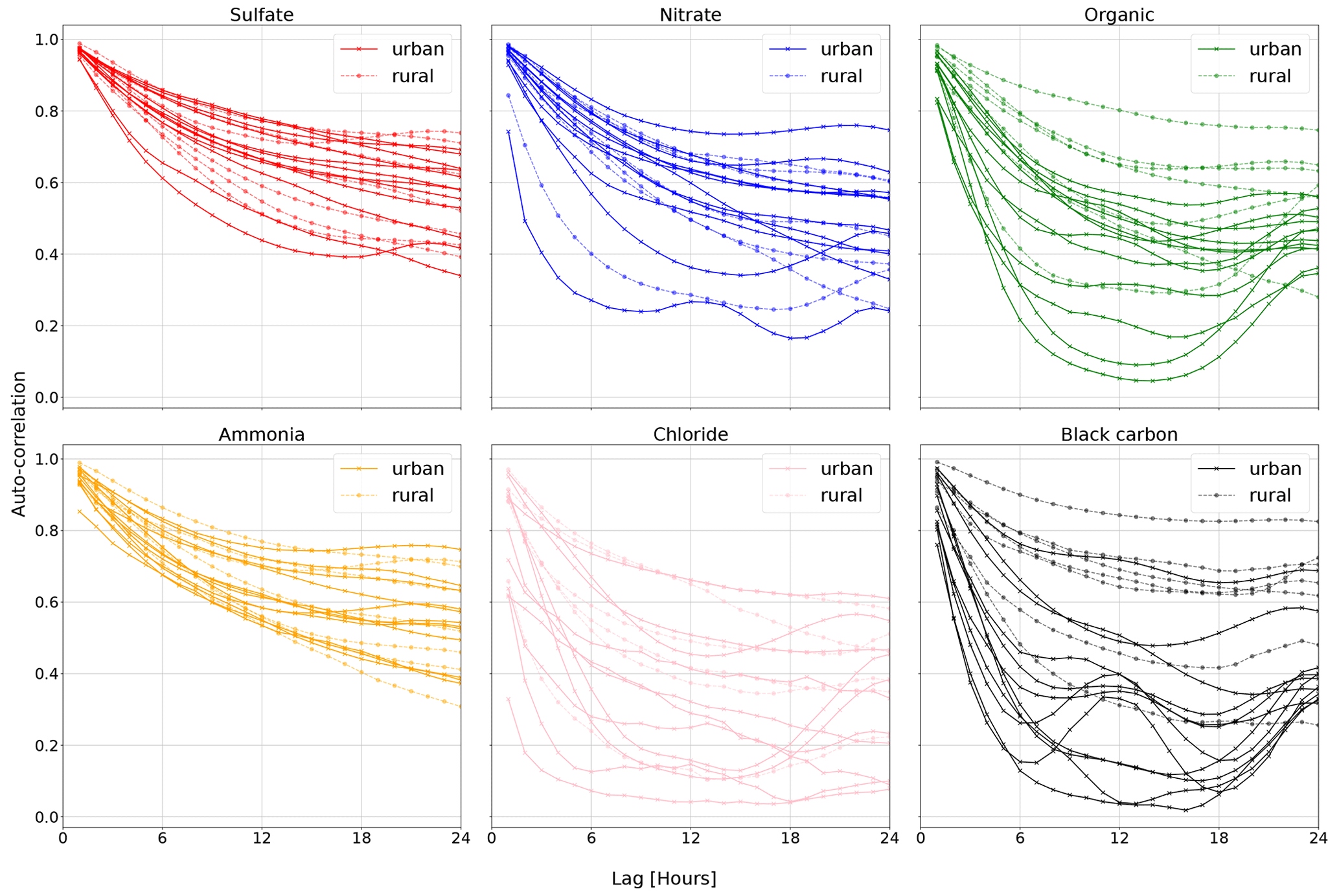
Figure 1The auto-correlations of the hourly means of several aerosol constituents measured at 19 different sites in Europe. The auto-correlation is the Pearson correlation coefficient between the original and the delayed time series. Auto-correlations at a lag of 1 and 2 h are very high in most cases. These data show that particulate matter constituents exhibit strong lag-1 auto-correlation, consistent with earlier such statements in the literature (e.g., Hirtzel et al., 1982). Auto-correlations calculated on data from Chen (2022).
In this section we discuss the methods used in the paper, starting with notation in Sect. 2.1. We define the BAMF model in Sect. 2.2 and describe how we find solutions in Sect. 2.3 using the pre- and post-processing steps in Sect. 2.4. In Sect. 2.5 we describe how we compare BAMF with PMF, which is defined in Sect. 2.6.
2.1 Notation
In this paper, we describe the data by , where the rows correspond to measurements taken at consecutive times ti. The columns correspond to the different dimensions of the measurement. Our objective is to find a lower dimensional non-negative decomposition X≈GF with p factors such that and , where . In other words, the objective is to present the data as a multiplication of two much smaller matrices. The rows of Fi⋅ contain the time-independent components of the decomposition, which we call factor profiles. Factor profiles are defined to sum to unity in order to facilitate comparisons between different datasets and models. The columns of G⋅i contain the time dependency of each of the rows of F; we will call these the factor time series. Simply put, the factor profiles represent the concentration and time-independent chemical composition of the sources, and the factor time series describes the time-dependent concentration of the sources. Note that the ordering of these profiles is arbitrary for the overall solution.
2.2 Bayesian auto-correlated matrix factorization, BAMF
We define a Bayesian probabilistic model that captures our prior assumptions of the process that generated the measurements. The only observed variables in our model are the data matrix and the uncertainty estimate . Together they define the probability distribution of the observed concentration of each at any point in time with the data matrix being the average and the uncertainty matrix the standard deviation of the distribution, here the Gaussian distribution. In addition to these observed variables, there are several latent variables. These include the matrices G and F mentioned above, vectors and which determine the auto-correlation behavior of the model, as well the “noise-free data matrix” . We define the probabilistic model as
where Normal corresponds to the normal probability distribution with a given mean and standard deviation, and Dirichlet to the Dirichlet distribution parameterized by a unit vector 1m. The model specification implies that the components of Fi⋅ can have values from [0,1] with equal likelihood, but all rows must sum to unity. Cauchy is the Cauchy probability distribution, with the width depending on the time difference between the ith and (i+1)th observation (). Essentially our model describes the data as a non-negative matrix decomposition (NMF) with a lag-1 auto-correlation term and a Gaussian error term for the reconstruction of X.
We chose the Cauchy distribution for the auto-correlation term because the long tails make large jumps between the ith and (i+1)th observation more probable than, e.g., a Gaussian distribution. Other choices are possible, but the experiments in this paper suggest the Cauchy distribution works as an approximation for real data. Choosing the distribution shape also implicitly influences the weight of the G auto-correlation. The αkΔti+βk determines the scale of the Cauchy distribution. The α terms allow the model to deal with time steps of different lengths and missing data, since it forms a simple linear model for the scale. It has a minimum width βk and increases linearly as Δt increases (with αk). Thus, for arbitrarily large time steps the Cauchy approaches a uniform distribution. In physical terms this means that at short time steps we expect the values of G to stay close to the previous value, and at large time steps larger deviations have higher probability. It is possible to use other formulations for the width, which would be appropriate if one wishes to include a more complex and computationally intensive description of auto-correlation. It is also possible to consider more than lag-1 auto-correlation.
2.2.1 Uncorrelated Bayesian matrix factorization, BAMF-0
For comparison, we created a version of the BAMF model without the lag-1 auto-correlation terms of Eq. (4). In other words, the model consist entirely of Eqs. (1)–(3). The model is otherwise identical to the BAMF model. This variation is essentially a probabilistic weighted NMF model, making it possible to assess the impact of the auto-correlation terms on the solution.
2.2.2 Bayesian matrix factorization with additional constraints, BAMF-C
In source apportionment analyses, it is common to utilize reference spectra as boundary conditions for the factor analysis – to find components with, e.g., previously observed chemical compositions. We include this scenario in another model, called “BAMF-C”, by adding peak intensity ratios to the BAMF model,
where ii, jj and kk, ll are the indices of matrix F indicating the peak pair to constrain. The ratio is the desired intensity ratio, and width is a free parameter describing the width of the distribution, i.e., the uncertainty of the intensity ratio. This approach makes it possible to constrain the range of F for arbitrarily many pairs, which is currently not done in the other models. A similar concept could constrain G to have a similar time behavior as an external ancillary measurement, e.g., of a source tracer. The constraint is similar to the widely used a value (anchor value) approach in Source Finder coupled to PMF (Canonaco et al., 2013, SoFi/PMF) with two notable differences. Firstly, the intensity ratio of the peaks is constrained in BAMF-C, while the a-value constraint approach in SoFi/PMF uses the peak intensity. Secondly, BAMF-C has a soft-boundary, with increasing penalty term as distance from the anchor grows. SoFi/PMF employs a hard boundary (defined as a relative deviation from the a value), without additional penalty on the object function Q for deviation from the anchor. In the present study, we evaluate the performance of the PMF and BAMF algorithm itself without discarding sub-optimal solutions (PMF) or samples (BAMF) during post-processing. Appendix F lists the profiles used for constraints in this work.
2.3 Solver
We use Stan (Carpenter et al., 2017) to compile and run the probabilistic models. Stan solves the probabilistic inference problem with a Markov chain Monte Carlo (MCMC) method. Instead of obtaining a single solution for the latent variables, e.g., by finding the model with the highest likelihood, we get an empirical distribution of possible solutions from which we can infer, e.g., confidence intervals. Stan takes our model and observed variables as input and outputs samples from the posterior distribution of the latent variables. We run multiple MCMC chains, starting from different initial conditions and usually extract a few thousand posterior samples per chain.
The standard way to initialize the model in Stan is by randomly sampling from the prior distributions. However, our model has many parameters with fairly strict distributions. Consequently, we found this starting point to be poor, sometimes causing Stan to markedly slow down, or even fail. Hence, we initialize the model with a point solution. We utilize Stan's capability to find a single maximum a posteriori (MAP) point solution for the parameters, which we use as the initialization. Note, however, that the solutions typically have several local optima, in which case the point solution is only one such local optimum.
Hamiltonian Markov chain Monte Carlo
Stan (Carpenter et al., 2017) uses a Hamiltonian MCMC method to draw samples from the posterior distribution of our model (Eqs. 1–4) given the data. We go through the basic idea here, but direct readers to Carpenter et al. (2017), Gelman et al. (2014) and references therein for a more detailed explanation.
The samples are drawn in proportion to the posterior probability of each sample. Obtaining samples from a multidimensional posterior distribution is a non-trivial task. For effective sampling, we use Hamiltonian Monte Carlo (HMC), a method where the gradient of the distribution and an ancillary variable called momentum are used to direct the chain to explore the typical set (Gelman et al., 2014). Specifically, we use the HMC based No-U-Turn Sampler (NUTS) (Hoffman and Gelman, 2014) from Stan. Stan uses warm-up iterations to estimate the parameters the NUTS sampler needs before drawing the posterior samples used in the computations (Carpenter et al., 2017).
The MAP estimate is used as a starting point for the sampling. It is found with an optimization method on the same probability distribution used by the sampling. We use the LBFGS (Liu and Nocedal, 1989) gradient-based optimization algorithm included in Stan for MAP estimates (Carpenter et al., 2017).
2.4 Pre- and post-processing
Before running our model, we normalize the data such that the mean of the data (X) is 1. The error estimate is scaled with the same scaling factor. The equations to do this are:
where fnorm is a scalar normalization factor, and are the scaled data and error, respectively, which we use as model inputs. This normalization is done so that we can use a consistent scale for priors and posteriors, making the modeling easier, and the denormalization is performed to return the results to familiar units. The normalization is optional, a user can also choose to use non-scaled values.
Stan outputs posterior samples from the two matrices F and G, representing the time-independent chemical composition of the factors and their time-dependent concentration. Since all the magnitude information is in G, G needs to be renormalized by simply multiplying with the normalization factor. The rows of F are constrained to sum to unity, and are, thus, directly comparable to mass spectrometric references, which are normalized similarly (Crippa et al., 2013; Ulbrich et al., 2022).
Sorting the components
The order of the components in F and G is arbitrary in our samples. The problem is not unique to BAMF but inherent to all such matrix decompositions. To be able to compare solutions, we need to be able to sort the components. The contribution of the same component to Z should be similar between two samples. To calculate the contribution for each component, we multiply the row of F with the corresponding column of G and use this to sort the components.
To select the ordering of the components, we take a small number of representative samples, usually the last five, and compute the optimal permutation using the Hungarian algorithm (Kuhn, 1955), which is a cost minimization algorithm that minimizes the cost of assigning values. In this case we are minimizing the Manhattan distances, which is the sum of absolute differences between the Z contributions in the samples. We then select the most common permutation as the ordering of the factors for all samples.
We use this approach for sorting the outputs of all models (BAMF-0/C, BAMF, PMF) to ensure the most direct comparability of the results. Finally, median, 25 %, and 75 % percentiles are computed using the sorted samples. In the comparisons, we use medians for all models, but in some figures, we also show 25 % and 75 % percentiles. The median, or any central estimate, is not guaranteed to be the “best” optimized solution in any metric (probability or root mean square sum of residuals). Still, we use it to represent a reasonable solution inferred from the samples.
2.5 Evaluating model performance
The first metric to check is if the model explains the data well (reconstruction performance). If X is not reconstructed appropriately, the solution is not acceptable. This can mean either that the data cannot be factorized this way (the model assumptions are wrong) or that the solver failed to find a solution. In such cases, the number of iterations should be increased, or solver parameters must be adjusted, such as the number of warm-up samples and parameters influencing the step size.
Even at moderate data sizes, assessing whether the original data falls within the model confidence bounds for every variable individually is not practical. Therefore, we summarized this information by computing the model residual (difference between the model input and output, mean of all samples) normalized with the uncertainty of the model output (standard deviation of all samples); essentially observing whether the original data are inside the sample standard deviation.
Data in S should be centered at 0 and have a standard deviation below 1, which means the data are often less than 1 model standard deviation away from the model mean. In addition, we also use a common evaluation metric in PMF analyses (), where Qm is defined as (Canonaco et al., 2013, notation adapted):
Essentially Qm describes the sum of squared model residuals normalized to the input error. We use the same reduction as Zhang et al. (2011) where Qexp is approximated as data size and denote as .
For synthetic data – with a known ground truth – it is possible to assess how well the methods resolve the actual components in addition to the reconstruction performance. We call this evaluation factorization performance. We compare the median solutions with the corresponding actual components by calculating the average distance, Pearson and Spearman (nonlinear) correlations. Optimal matching between median solutions and true components is obtained using the Hungarian algorithm (Kuhn, 1955). The approach is similar to the sorting above but with the true components defining the order. Direct comparison with true components is only possible in cases where the number of true components matches the number of modeled components. Otherwise, the model must combine multiple components or create additional ones.
2.6 PMF
We use PMF, specifically the multilinear engine 2 (ME-2) controlled by the user interface SoFi (Canonaco et al., 2013; Paatero and Tapper, 1994), as a baseline comparison. PMF solves the decomposition in Eq. (1) by minimizing the sum of the squared residuals normalized with the input error – see Eq. (7) (object function) – given the boundary condition that all values must be positive (Canonaco et al., 2013). Since SoFi finds local optima, we ran it with different random seeds to get multiple solutions for all comparisons. As the runs have varying starting points, they often lead to different local optima, especially in cases with high rotational ambiguity. Thus, PMF provides a collection of local minima, while BAMF tries to sample the posterior distribution of the model, including plausible answers that are not minima. For simplicity, we will refer to the group of PMF solution sets as “samples”, even though PMF is not a sampler.
A priori information in the form of known rows of factor profiles or of known columns of factor time series can be added to the model to reduce the rotational ambiguity. By adding this external information, the user can reduce the space PMF searches for the optimized solution, reducing the rotational ambiguity of the solution. Using external data to run PMF is usually referred to as “constraining the solution”, and external information is used as constraints. Here we used two approaches, (a) entirely unconstrained PMF runs and (b) constrained runs using external source profiles. We rely on the commonly used a-value approach to constrain the PMF runs. In the a-value approach, the user inputs one or more factor profiles or factor time series and defines a relative tolerated deviation from the anchor (termed “a value”) (Canonaco et al., 2013). Constraint strengths are not directly comparable between the hard cut-off approach used in PMF and the softer Gaussian error term approach used in BAMF-C. For the best possible comparability, we first ran BAMF-C (constraint strength 0.001) and determined the equivalent a value by taking the maximum deviation from the anchor value on a constrained component in F (a value of 18 %). See Appendix F for the profiles used to make this comparison.
We generated synthetic datasets mimicking the OA sources in different urban environments. These synthetic datasets mimic mass spectral OA analyses of a Time-of-Flight Aerosol Chemical Speciation Monitor (ToF-ACSM, Fröhlich et al., 2013), a ubiquitous instrument in measuring PM composition with a focus on OA. The instrument measures a signal for several mass-to-charge ratio channels. We model these mass spectra as a sum of 2–5 different mixed sources. The sources are constructed of time-independent chemical fingerprints, in our notation F, from the AMS Spectral Database (Ulbrich et al., 2009, 2022) combined with their time behavior and magnitude, G. The noiseless spectra, Z, are then acquired by matrix multiplication of F and G. We then generate X, as Eq. (2), by applying random Gaussian noise to each data point. The errors are applied to X, which is a sum of all the components, so that individual component error in the original G is undefined.
The ToF-ACSM alternates between measuring particles and air together, called “open signal” (Iopen), and measuring only air, called “closed signal” (Iclosed). The difference signal () represents the signal caused by the measured particles. For computing the error of Idiff, we use an error function based on the signal strength, according to Allan et al. (2003), and Ulbrich et al. (2009):
where topen and tclosed are the open and closed signal measurement times, respectively, is the mass charge ratio of the measurement, Errormin is a lower limit set on the measurement error, and Ibaseline is the baseline signal in the mass spectrometer. Since the organic fragment ions at the values 16, 17, 18, and 28 are computed based on the measurement at 44 and thus contain duplicate information, they are removed before running any of the models and only later reintroduced in the results.
3.1 Synthetic data representing a polluted megacity
First, we generated a synthetic ToF-ACSM OA mass spectral dataset mimicking a polluted megacity environment affected by multiple OA sources. The synthetic datasets used here are based on observations from Beijing, as it is a relatively well-studied environment. In our case, the modeled sources are traffic exhaust (HOA); cooking (COA); biomass burning (BBOA); coal combustion (CCOA); and secondary OA (OOA). In addition, we also constructed more simple datasets generated with fewer factors (two factors: HOA + OOA; three factors: HOA+COA+OOA; and four factors: HOA+COA+BBOA+OOA). F were chemical fingerprints from the literature (Elser et al., 2016; Ulbrich et al., 2009, 2022). G was created as a mix of Gaussian and Cauchy (BBOA Gaussian, others Cauchy), biased, positive random walks, with added typical diurnal concentration cycles (Kulmala et al., 2021) corresponding to the matching OA sources (based on F). A mix of different random walk distributions was chosen to test whether the model approximation of Cauchy auto-correlation works with them. The random walk aims to introduce variability such as one would get from varying transport and mixing. The diurnal cycle was simply summed to the random walk to produce the time series. The overall order of magnitude and diurnal concentration variability of the components (OA sources) were estimated based on previous literature on OA sources in Beijing (Kulmala et al., 2021). For each number of factors, we constructed 10 different datasets amounting to a total of 40 datasets. For reference, one 5-component dataset in its component form is shown in Fig. 2. CCOA and BBOA are very similar in F and G (see Appendix B), making it a challenging dataset. The time series of CCOA and BBOA are also similar in magnitude and have similar diurnal behavior. While the short-term auto-correlation is high, the random walks of the megacity dataset are not as highly auto-correlated as the PM data in Fig. 1. The added diurnal peaks can be seen as the periodic peaks in the correlograms in Fig. 2c and f. See Appendix C for an example of the dependence of the measurement errors on this dataset.
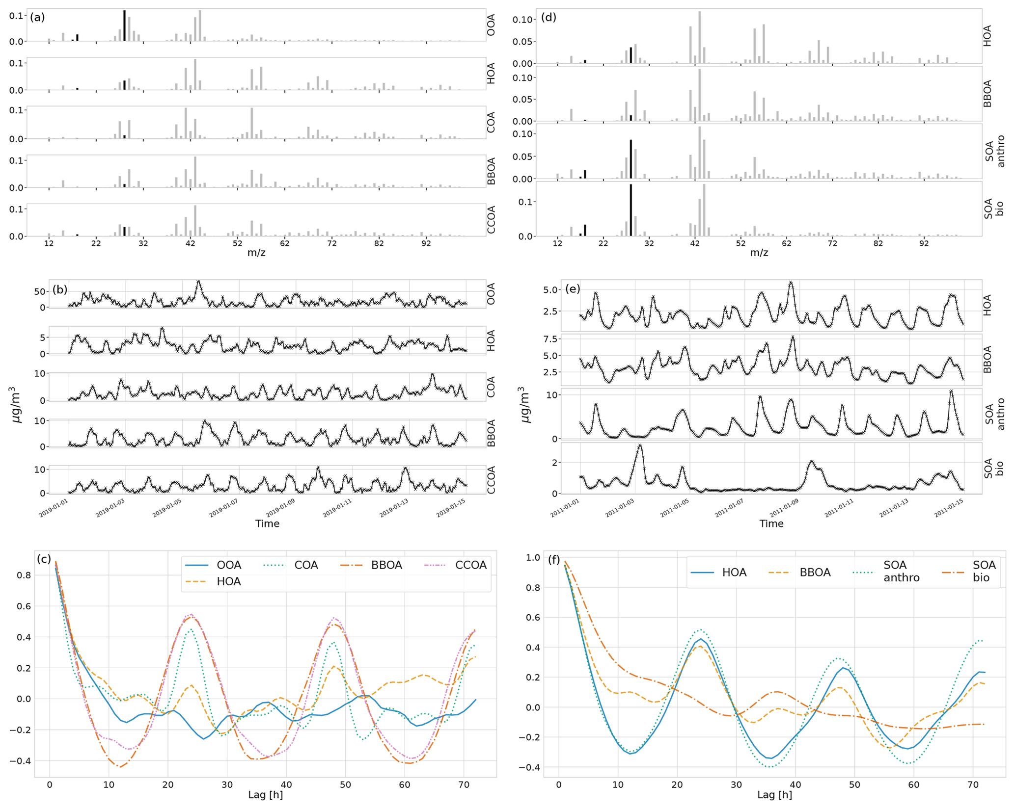
Figure 2Characteristics of the synthetic ToF-ACSM OA datasets. Panels (a) and (d) show the factor profiles (F) used to construct the synthetic datasets. The solid black bars are ions derived from 44 and are only used for converting concentrations. Panels (b) and (e) show the factor time series (G) used to construct each dataset, and the unit for them is µg m−3, and panels (c) and (f) show the temporal auto-correlation for each factor. Auto-correlation refers to the Pearson correlation coefficient of the component with the same component time-shifted by the number of hours. Panels (a), (b), and (c) are for megacity data and panels (d), (e), and (f) are for the European urban environment.
3.2 Synthetic dataset representing a typical European urban environment
As another test, we used chemical transport model data from Jiang et al. (2019) representing approximately 2 weeks of simulated measurements in Zurich, Switzerland. Zurich represents a typical European city with low pollution levels. In this case, the G time series come from the transport model and F is taken from the literature (HOA and BBOA from an ambient analysis presented by Elser et al., 2016; Ulbrich et al., 2009, 2022, biological SOA (SOAbio) from an ambient analysis presented by Daellenbach et al., 2017, anthropogenic SOA, SOAanthro, is represented by laboratory Diesel generator SOA presented by Sage et al., 2008).
This dataset differs from those in Sect. 3.1 in two important ways. Firstly, the concentrations are lower since the environment is less polluted, which affects the error estimation as larger relative measurement errors, median 1.0 % of data magnitude for this dataset and median 0.6 % for one of the datasets described in Sect. 3.1. Secondly, the sources exhibit high correlation in the time series (Appendix B shows that correlations in G are higher than in the dataset described in Sect. 3.1), possibly indicating that meteorological conditions and transport of pollutants are important drivers of the concentration of the components. From a source apportionment analysis perspective, this simulates the worst-case situation with the data having poor separability in G. The components of this dataset compared to the megacity data can be seen in Fig. 2. The auto-correlation behavior of the two datasets is very similar, indicating that our fully synthetic data behave as realistically as the transport model.
In this section we compare the factorizations from BAMF and PMF on simulated megacity data, in Sect. 4.1, and synthetic European data, in Sect. 4.2. We also investigate what happens when we do not know the true number of sources, in Sect. 4.3, and how additional prior information improves the factorization, in Sect. 4.4.
4.1 Simulated megacity source apportionment
In the first experiment, we assess the performance of BAMF, BAMF-0, and PMF on synthetic data mimicking the conditions in a polluted megacity described in Sect. 3.1. First, we assess the reconstruction of the input by the different models. In addition to minimizing the residuals, BAMF also includes a penalty for deviations from auto-correlation in G. Due to this and BAMF being a sampled model instead of an optimizer as described in Sect. 2.3, PMF would be expected to give answers with lower absolute measurement error-weighted residuals compared to BAMF. In other words, PMF is expected to have a better reconstruction performance.
Figure 3 shows the median solution reconstruction across the 10 different datasets as the number of components increases. All models reconstruct the input data well within the error estimate. The similar reconstruction metrics for BAMF and BAMF-0 suggest that the inclusion of the auto-correlation term does not substantially deteriorate the reconstruction accuracy. On the other hand, PMF has, as expected, marginally lower absolute measurement error-weighted residuals than BAMF and BAMF-0. However, they are below unity and within the error estimate, judging by the normalized residuals. Therefore, PMF most likely finds solutions that fit the noise in the data better. All other reconstruction metrics (S mean, S standard deviation, ) are comparable for all models.
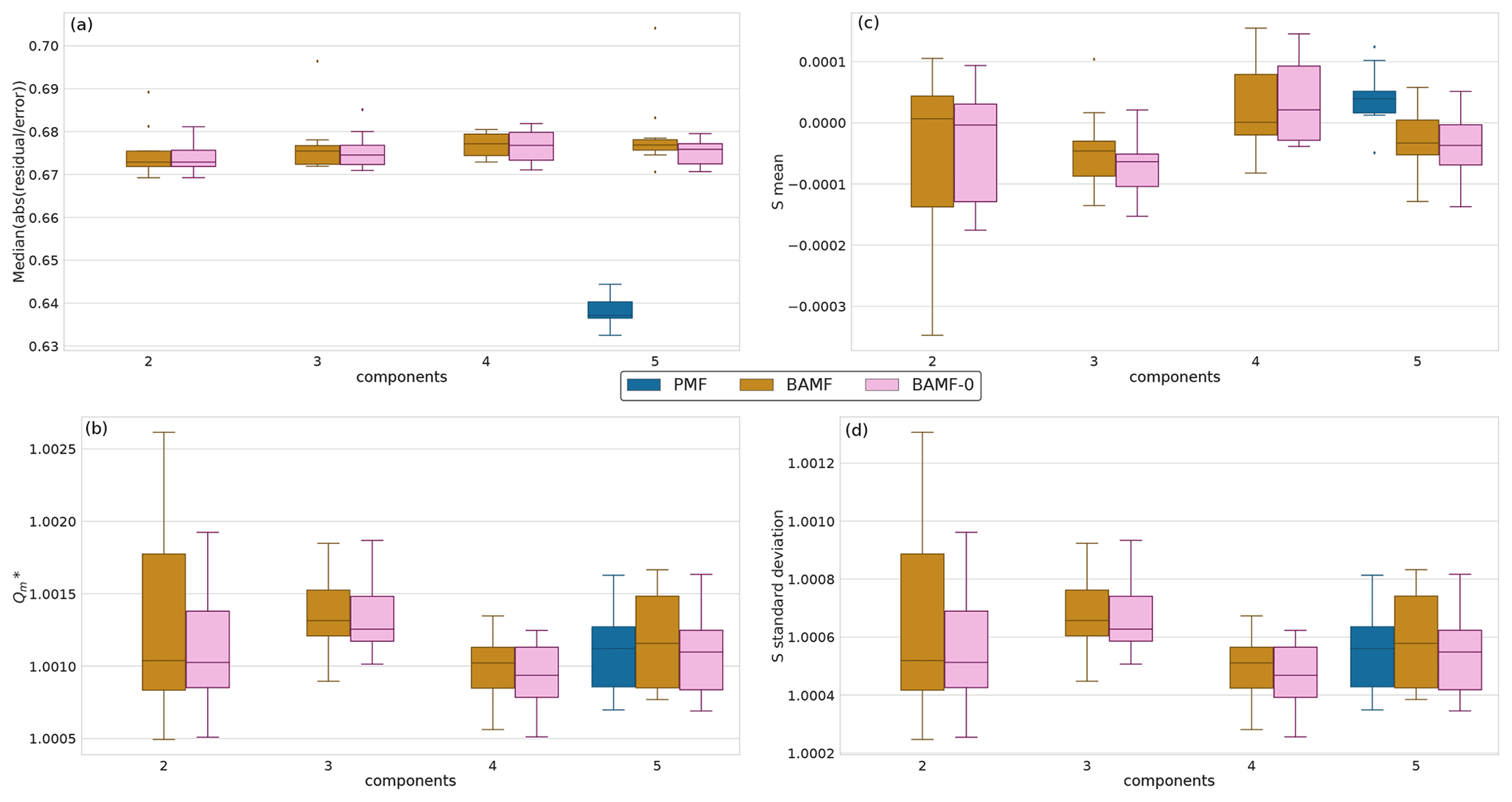
Figure 3Reconstruction metrics for BAMF, BAMF-0, and PMF for synthetic megacity data. Panel (a) shows the relative error of X of the median solution as a function of the number of components for the synthetic megacity data (BAMF and BAMF-0: results from 10 different datasets for each number of factors, PMF: only for the 5-factor cases). Panel (b) shows the statistic, where all models are very similar. Panel (c) shows the mean and panel (d) shows the standard deviation of S, as a function of the number of factors for the synthetic megacity data (the ideal value for the mean is 0 and the ideal value for standard deviation is smaller than 1). S refers to the difference between the original data and the samples normalized with the standard deviation of the samples (uncertainty of the model).
Data reconstruction is essential to get within the error limits. However, source apportionment aims to accurately and precisely resolve the actual components in G and F, i.e., factorization performance. The solution of each model to the example dataset is shown in Fig. 4. For this example, we observe that all models resolve all five components. However, BAMF has a better factorization performance both in F and G than the models not accounting for auto-correlation (BAMF-0, PMF) in Table 1. Similarly, for the diurnal cycles in the example in Fig. 4c, the diurnal concentration of OA sources, as identified by BAMF, closely resembles the ground truth components. While all models capture the time behavior of the diurnals, the absolute magnitude has a bias, with BAMF having a substantially smaller bias than the other models for four out of five components (Table 1).
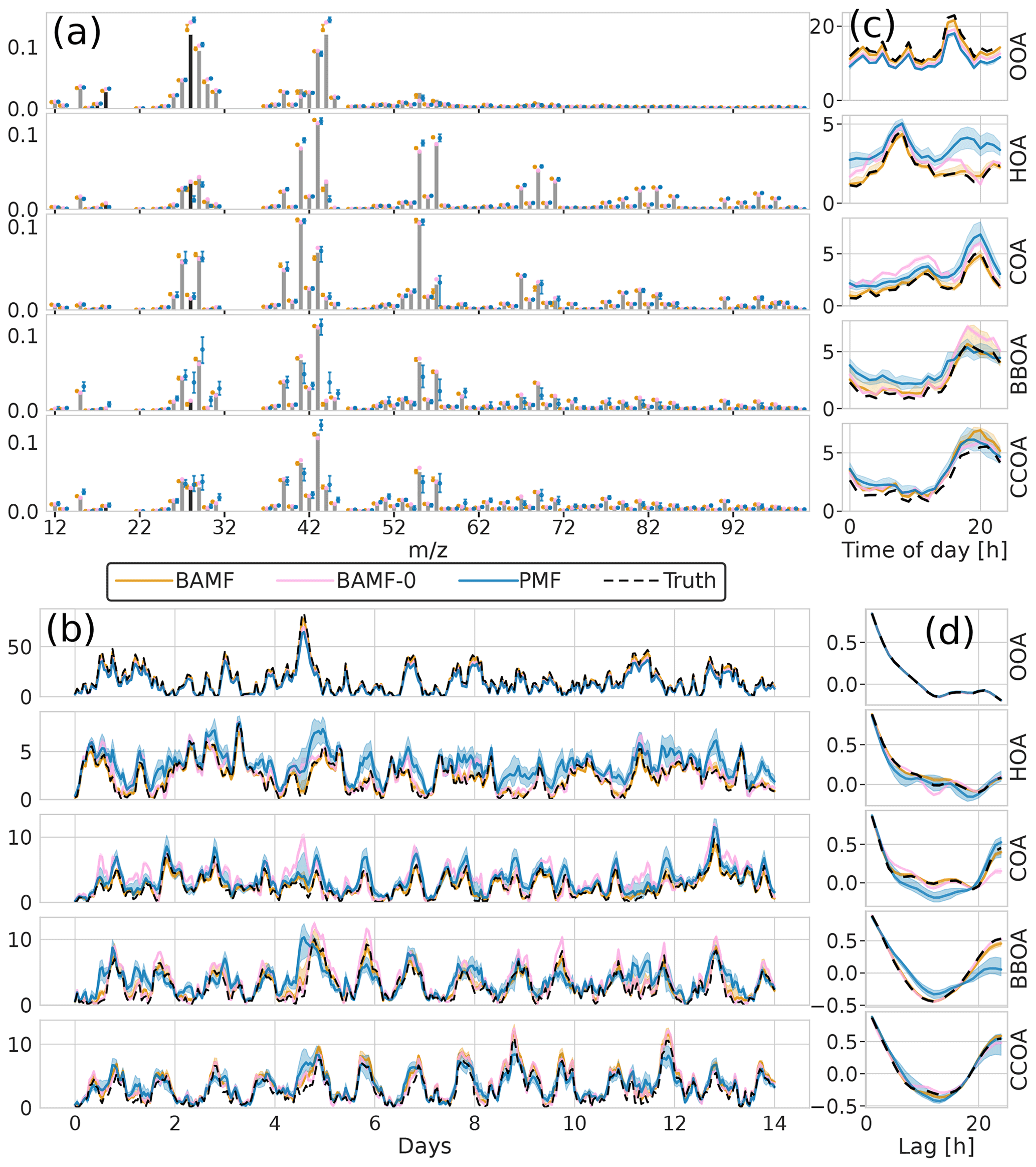
Figure 4Illustration of F and G reconstruction of all models for one of the synthetic megacity ToF-ACSM OA datasets with five components. Panel (a) is F, (b) is G, (c) is the diurnal concentration variation, and (d) is auto-correlation measured as Pearson correlation coefficient. Here, we display the median and the 0.25 and 0.75 quantiles. For all BAMF-type models, these quantities are computed based on the samples and for PMF, based on the 100 solutions.
Table 1Reconstruction and factorization performance of all three models for the synthetic megacity ToF-ACSM OA dataset in Fig. 4. The reconstruction metrics measure the residuals divided by the error estimate. A value closer to 0 is better and a value below 1 is smaller than the error estimate given to the model. The factorization performance is assessed via three metrics: Truth is the average ratio of each factor time series, r is the Pearson correlation coefficient between the factor time series, and ρ is the Spearman correlation coefficient between the factor profiles. For the factorization performance, a value closer to 1 is better. Nonlinear correlation coefficient is used for factor profiles, since they have an additional constraint of summing to unity and thus linear correlation is penalized for small errors disproportionately. For each metric, the best value is highlighted in bold.
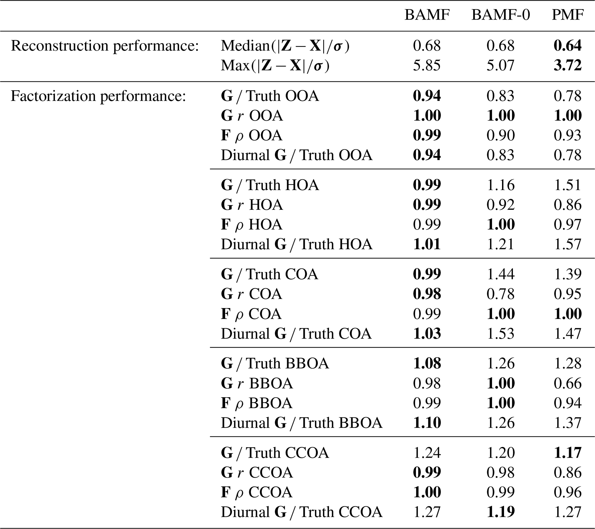
All models slightly underestimate OOA, which results in overestimating the other components (Table 1). For the final component, CCOA, PMF has less bias, but it correlates worse with the truth. BAMF-0 and PMF significantly underestimate OOA, which results in an overestimation of other components to get the reconstruction correct. Some factors have a more pronounced cyclical temporal behavior, as witnessed by high auto-correlation at higher temporal lag (e.g., Fig. 4c CCOA, BBOA, COA). Based on Table 1, some of the factors with pronounced cyclical temporal behavior are better represented by BAMF than PMF (e.g., BBOA, COA), while this is not necessarily the case for others (e.g., CCOA).
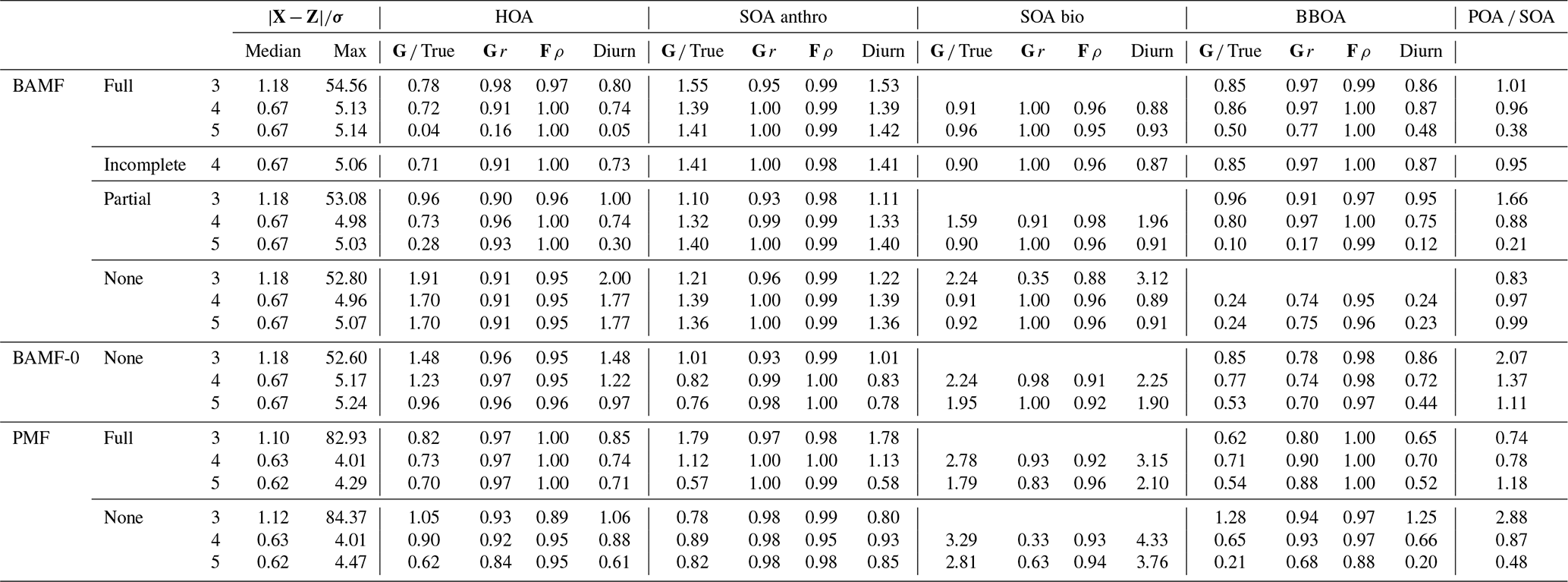
Table 2Reconstruction and factorization performance for the synthetic European city ToF-ACSM OA dataset. True is the average ratio of the component to the true one, r is the Pearson correlation coefficient, and ρ is the Spearman correlation coefficient. Diurn is a factor's average ratio of the diurnal of G to the true diurnal. POA SOA is the ratio of primary (HOA, BBOA) and secondary organic aerosol (anthropogenic SOA, biogenic SOA); for the ground truth, this ratio is 1.55. Unidentified components were not included in this ratio. For the reconstruction metrics, values closer to 0 are better, and values below 1 are within the error given to the model. For factorization metrics, the ideal value is 1.
When considering all 10 synthetic datasets with five components mimicking a polluted megacity, BAMF consistently produces factors closer in magnitude to the truth and which correlate better with the actual factors than the other models (Fig. 5). BAMF is also better correlated with the time behavior of the components, while one of the components (CCOA, strongly correlated with BBOA in terms of G and F) is difficult for all models. We hypothesize BAMF-0 shows better spread in Fig. 5, due to being constrained by the underestimation of OOA and having to include those peaks in the spectra. Figure 5a shows that BAMF can over- and underestimate both BBOA and CCOA depending on the dataset. Appendix A shows the inverse relationship between CCOA and BBOA mass concentration biases and how the profile reconstruction affects the CCOA mass concentration bias for the BAMF model. Overall, using auto-correlation in source apportionment markedly improves the quality of the resolved factors while keeping the overall reconstruction metrics similar.
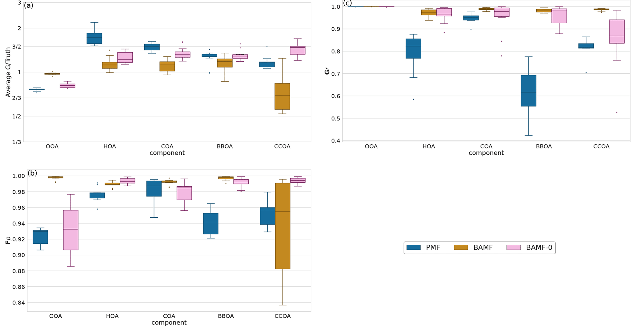
Figure 5Summary of factorization performance of the three models for all synthetic megacity ToF-ACSM OA datasets with five components (10 datasets): Panel (a) shows the mean of the median value of the components of G divided by the true value (ideal value is 1). Panel (b) shows the Spearman correlation coefficient median solution components of F compared to the true value (a value of 1 refers to a perfect correlation). Panel (c) shows the Pearson correlation coefficient of the median solution components of G compared to the true value (a value of 1 refers to a perfect linear correlation).
4.2 Simulated European low-pollution city source apportionment
In a second exercise, we assessed the performance of BAMF, BAMF-0, and PMF on a synthetic dataset mimicking the conditions in a typical European city (Sect. 3.2). In contrast to the fully synthetic dataset in Sect. 3.1, here, the true components G are OA source components computed by an air quality model (Jiang et al., 2019). This provides G time series close to the atmosphere while still knowing the ground truth. While the three models show somewhat different components (Fig. 6), the reconstruction metrics indicate that all models have acceptable solutions (Table 2). In fact, the metrics also show that the European dataset is reconstructed almost within the error limits with even only three components, i.e., one component less than is present in the synthetic dataset (HOA, BBOA, SOAanthro, SOAbio). This could explain why there is significant freedom in acceptable four-component solutions and variation between them.
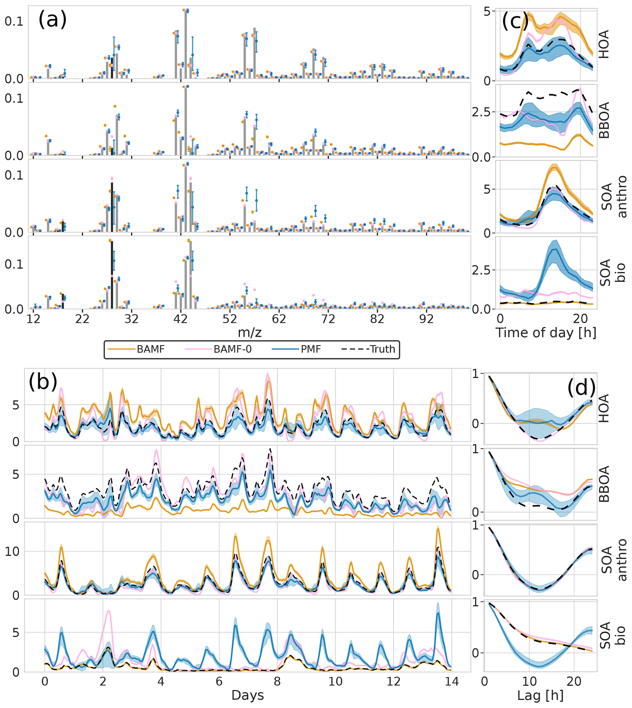
Figure 6Factorization performance of all three models for the synthetic European city ToF-ACSM OA dataset. The shaded area is the interquartile range (0.25–0.75 quantile). Panel (a) is F, (b) is G, (c) is the diurnal, and (d) is auto-correlation measured as Pearson correlation coefficient.
All models show signs of mixing between the components, most likely due to the correlation of the true G components (time behavior is very similar) as well as similar chemical signatures F. PMF mixes the SOA components while BAMF mixes the POA components. However, it is worth noting that BAMF has a significant bias on several components in G as seen in Table 2, but otherwise reflects their time behavior well. Given the recovered POA SOA ratio, BAMF most likely mixes HOA and BBOA explaining that HOA is overestimated while BBOA is underestimated. PMF, on the other hand, produces two almost identical components (both in F and G) for two of the four components, and PMF cannot thus distinguish the components present in the dataset. In Fig. 6d BAMF-0 and BAMF also seem to overestimate higher lag auto-correlation of BBOA in a similar fashion but have a higher bias. It should be noted that even BAMF only considers lag-1 auto-correlation in the model. For HOA, BAMF and PMF do not match the anti-correlated part between lags 5 and 20 and PMF cannot match the behavior of SOA bio. Overall, all models are challenged by the European dataset, with BAMF having the most consistent performance.
4.3 Resolving an unknown number of sources
For real-world source apportionment analyses, the true number of components, i.e., sources, to be resolved via matrix factorization is unknown yet crucial. Despite the importance, accurately determining and specifying the correct number of modeled components is not trivial (see, e.g., Isokääntä et al., 2020; Ulbrich et al., 2009; Zhang et al., 2011). Typical strategies rely on reconstructing X within the measurement error, the absence of structure in the measurement error-weighted residuals and the environmental interpretability of the resolved components. Here, we assess the behavior of the BAMF, BAMF-0, and PMF models as the number of components are changed on the four-component chemical transport model dataset from Sect. 3.2. The model runs were performed both with an underspecified setting using three components and overspecified setting using five components (Figs. 7 and 8). While underspecified, all models extract an SOAanthro component and merge the remaining three components into two. At the same time, BAMF extracts a component similar to SOAbio, while BAMF-0 and PMF extract components similar to HOA and BBOA but lack SOAbio.
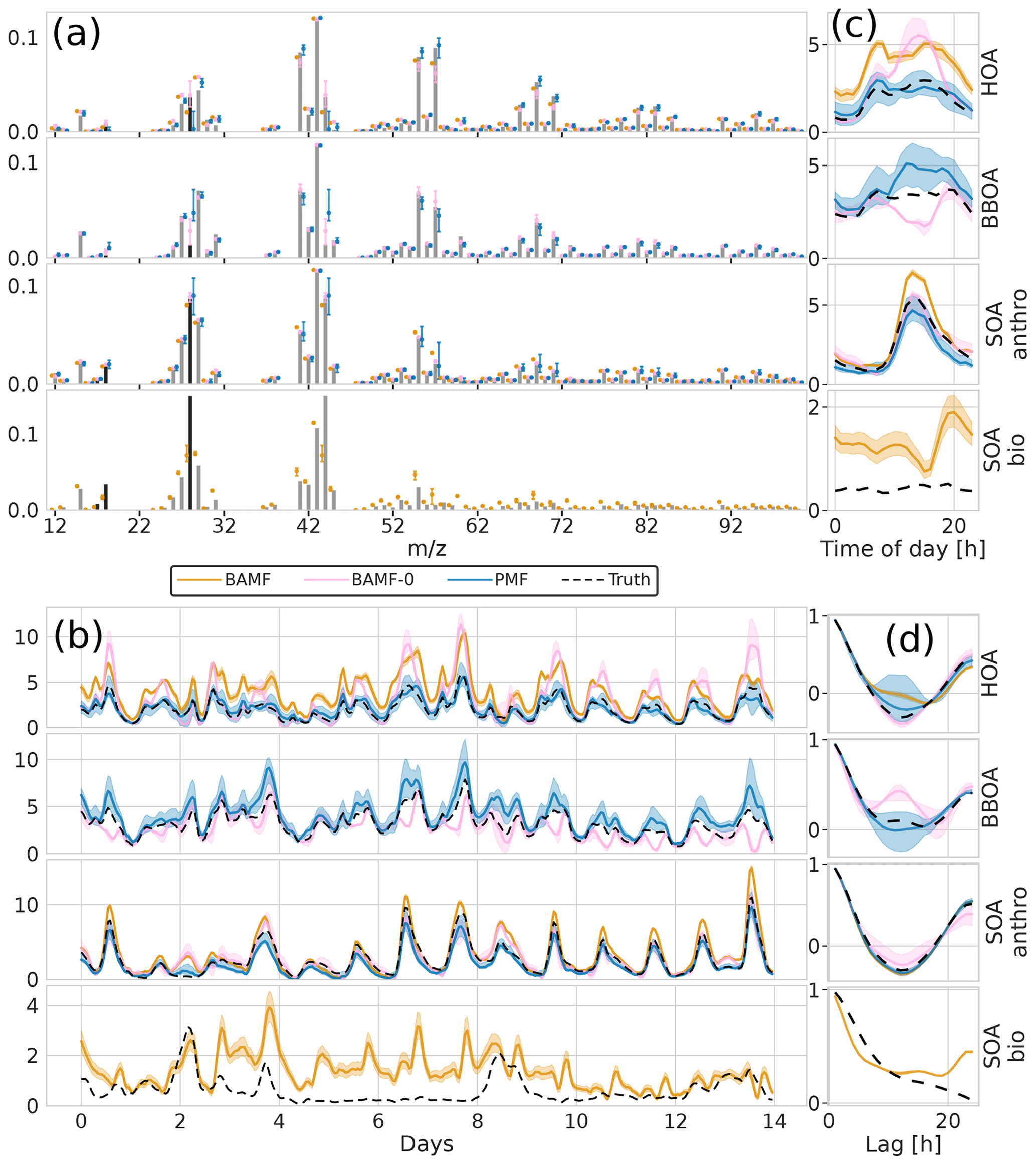
Figure 7Factorization performance of underspecified (three components) models for the synthetic European city ToF-ACSM OA dataset. Panel (a) is F, (b) is G, (c) is the diurnal, and (d) is auto-correlation measured as Pearson correlation coefficient. The models extract different components and they are shown next to the closest original component. This is why there are 4 components shown even though the models extract only 3 components each.
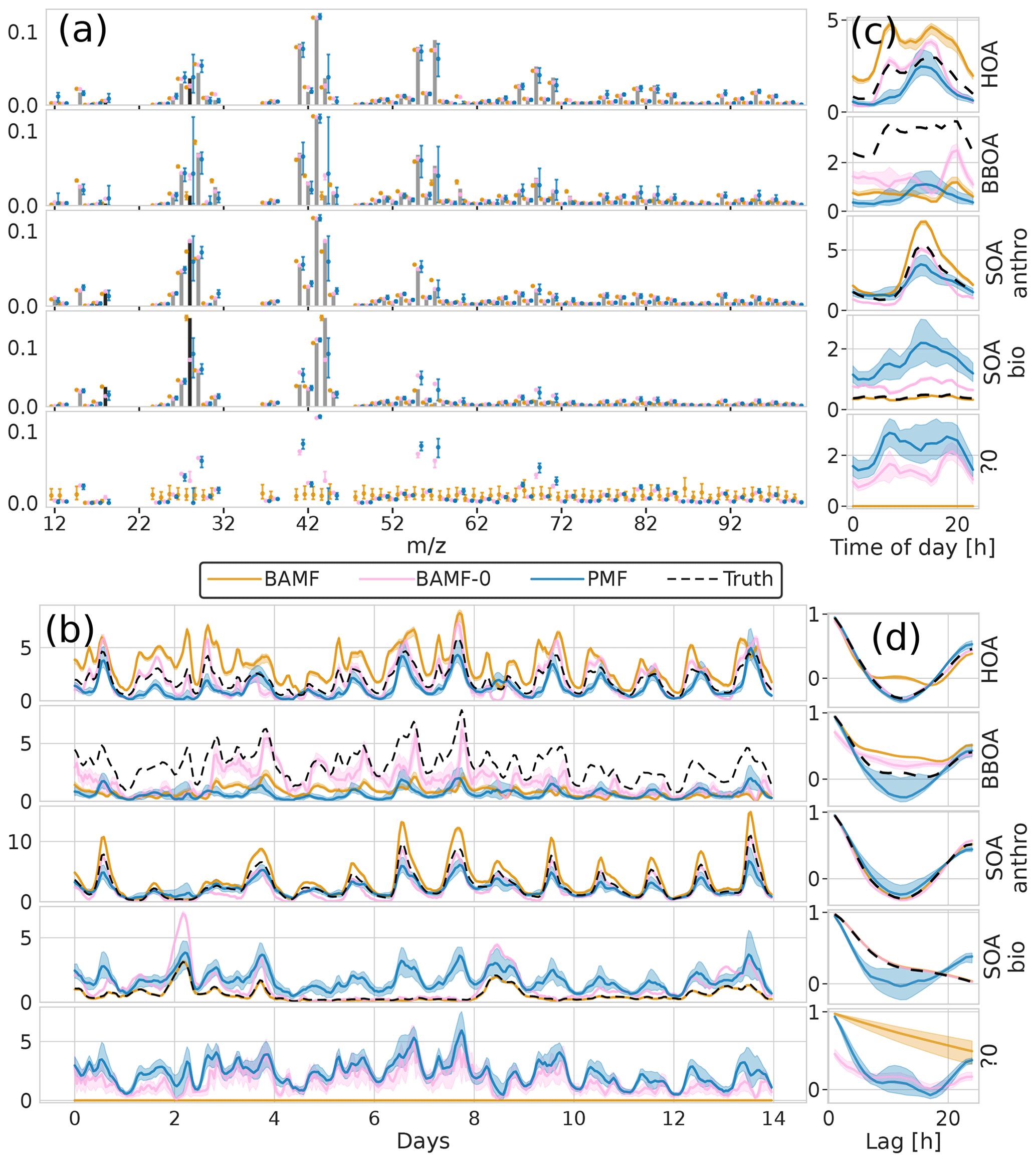
Figure 8Factorization performance of overspecified (five components) models for the synthetic European city ToF-ACSM OA dataset. Panel (a) is F, (b) is G, (c) is the diurnal, and (d) is auto-correlation measured as Pearson correlation coefficient. “?0” denotes an unidentified component.
For the overspecified models (five instead of four components), the results differ (Fig. 8). While the models without the auto-correlation assumption (PMF, BAMF-0) split the true components into multiple sub-components (mostly the POA components, HOA and BBOA), BAMF produces an extra component that is easily identifiable as unnecessary in addition to the four components resolved with four factors. This unnecessary component is characterized by an extremely high auto-correlation and low magnitude, as seen in Fig. 8b, c, and d. For this component the time series is almost constant, and the composition is flat with large uncertainties. The extra component does not affect the factorization performance of the other components of BAMF substantially. At the same time, BAMF-0 and PMF have a reduced factorization performance with too many components (Fig. 8, Table 2). In general use, one would prefer the model to indicate the limits of the factorization as BAMF does, instead of producing duplicate components. It should be noted that the behavior of BAMF can be changed by adding new model terms, such as constraints on F. For example, the model minimizes the constrained component when it is run equally overspecified (five instead of four components) but with a priori information on F as can be seen in Appendix D.
4.4 Using ancillary information to improve resolving sources
As highlighted in Sect. 4.2, all models are challenged by the European dataset. Imperfect matrix factorization results are likewise often observed when using PMF for real-world chemical datasets (see, e.g., Canonaco et al., 2013; Daellenbach et al., 2017). Often, information is available that could help resolve the sources, such as chemical fingerprints of specific components associated with different sources. In current practice, previously observed F profiles are often used as boundary conditions in source apportionment analyses. This approach has significant uncertainty in the general case because true F is unknown. Still, in our specific test case, the a priori information is precisely correct – the known information on F of the true components.
We tested the performance of the models when using a priori information on F using three different approaches on the European dataset (from Sect. 3.2):
-
Full constraint. For BAMF-C and PMF, the two POA components (HOA and BBOA) were fully (for all s) constrained with a roughly 18 % deviation allowed from the anchor (see Sect. 2.2.2 and 2.6 for the determination of this).
-
Incomplete constraint. Knowledge on the entire factor profile is not always available, e.g., not the same range is measured. With the incomplete constraint approach, we test whether a priori information on parts of the factor profile improves the factorization performance and thus whether such information is useful. For the BAMF model, a priori information was only used in a limited arbitrarily chosen range (12–60) instead of for all s ( 12–100), the same deviation allowed from the anchor for the constrained components.
-
Partial constraint. Sometimes, only very little chemical information is available for a specific factor, and it is defined by few key tracers. With the partial constraint, we test whether a priori information on just a few peaks/variables improves the factorization performance. For the BAMF model, a priori information was only used for four arbitrarily chosen peaks out of 74 (s 45, 57, and 60, F[ii,jj], compared to 43, F[kk,ll]) for HOA and BBOA defined with the same deviation allowed from the anchor for constrained components.
The reconstruction and factorization performance of the different models are compared in Table 2. The fully constrained BAMF model (BAMF-C) performs substantially better in extracting BBOA both in F and G compared to BAMF. In fact, the extracted components are very similar to the true components with very similar temporal behavior and reduced biases in G (Fig. 9). Fully constrained PMF performs marginally better than unconstrained PMF but still mixes SOAbio with SOAanthro (Fig. 9). This can be expected since the a priori information is applied to HOA and BBOA, not to the SOA components. Figure 9d shows that PMF-C captures HOA time behavior very well, while BAMF still overestimates some auto-correlation, even though the bias in Fig. 9a is significantly reduced. PMF-C also has some solutions that start to approach correct SOA bio, with solutions falling between unconstrained PMF and BAMF-C. For BAMF-C and BAMF SOA bio is virtually unchanged (Figs. 9a, d and 6a, d). The incompletely constrained BAMF model performs slightly worse than the fully constrained BAMF model. Partially constrained BAMF performs worse but is still on par with the fully constrained PMF (Table 2). The partially constrained BAMF model reduces bias in BBOA but starts mixing SOA bio with the other components (Fig. 10, Table 2). Using a priori information on F improves the factorization performance of both PMF and especially BAMF, with more information leading to solutions closer to the ground truth. This is especially helpful when the additional information is on the components the model mixes when unconstrained. Such prior information is powerful, e.g., constrained PMF does better than unconstrained BAMF for all components except SOA bio. For this dataset and these constraints, BAMF-C fully constrained has the best factorization performance, fully constrained PMF and partially constrained BAMF-C perform slightly worse but about equally good, and unconstrained models fail to resolve one or more components correctly regardless of the model. A comparison of the results of fully constrained PMF and unconstrained BAMF can be seen in Appendix G.
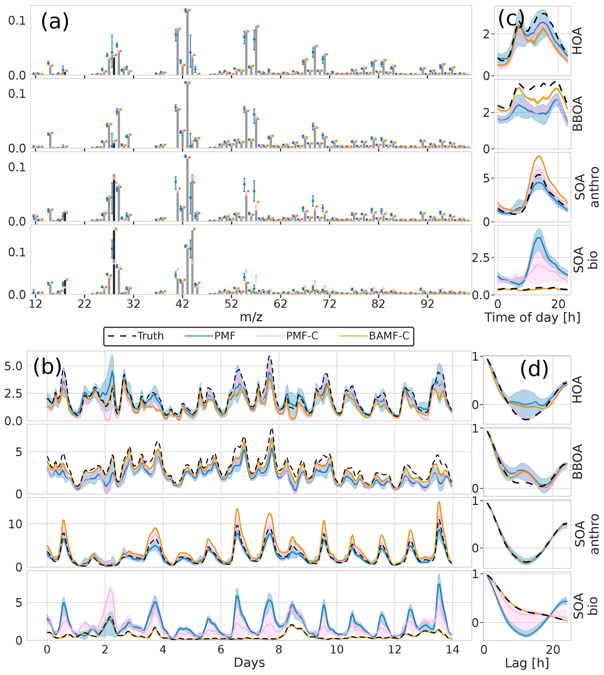
Figure 9Factorization performance of models using a priori information on F for the synthetic European city ToF-ACSM OA dataset, fully constrained BAMF and fully constrained PMF results compared to unconstrained PMF. Panel (a) is F, (b) is G, (c) is the diurnal concentration, and (d) is the auto-correlation behavior.
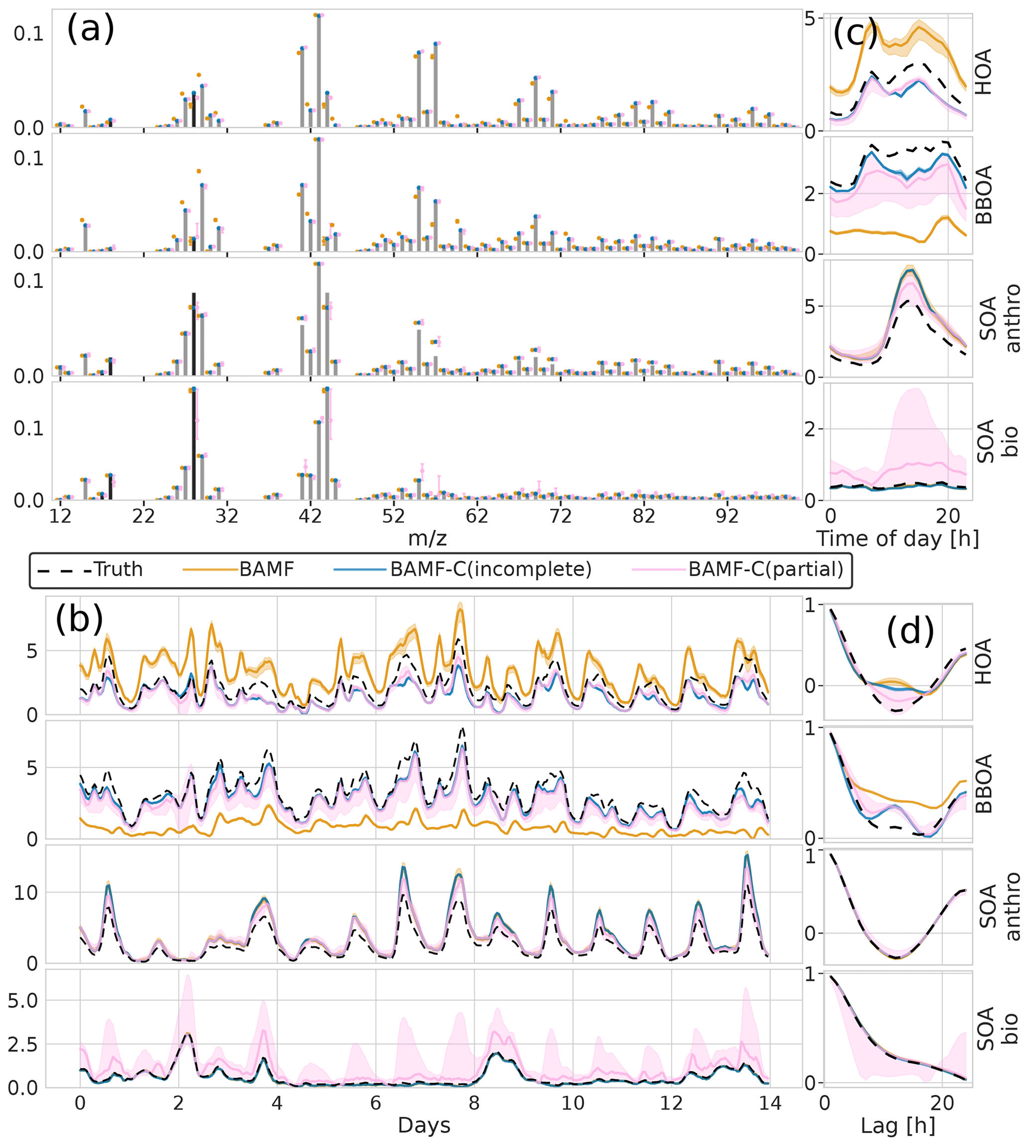
Figure 10Factorization performance of models using a priori information on F for the synthetic European city ToF-ACSM OA dataset, partial and incomplete constraints in BAMF compared to unconstrained BAMF. Panel (a) is F, (b) is G, (c) is the diurnal concentration, and (d) is the auto-correlation behavior. The results for SOA components overlap between BAMF and BAMF-C(incomplete) such that the BAMF results are not visible in panels (b), (c), and (d).
We present a Bayesian matrix factorization model that accounts for temporal auto-correlation of the components (BAMF) and provides direct error estimation. BAMF is built on top of Stan, a freely available, robust, actively developed, open-source framework for statistical modeling with the ability of full Bayesian statistical inference with MCMC sampling. Here, we characterize the BAMF performance on synthetic Time-of-Flight Aerosol Chemical Speciation Monitor mass spectral OA data compared to PMF. This approach allows us to assess the model performance based on input data reconstruction and the ability to accurately model the chemical composition and concentration time series of the components.
All models performed well in reconstruction performance regardless of factorization performance, indicating that reconstructing the data is insufficient for judging how good the extracted factors are. Without strongly correlated components, BAMF resolves temporally auto-correlated components well (synthetic megacity dataset), while PMF performs considerably worse. Both BAMF and PMF are challenged by strongly correlated components (European data).
Further, we show that using a priori information on the chemical composition of the components improves BAMF factorization performance such that all components are well represented. Even adding a priori information for a few peaks significantly reduced component bias, and partially specifying the profile (for 56 % of the peaks) produced comparable results to fully constraining the profile with PMF. This opens up possibilities for using incomplete chemical composition information to improve factorizations.
While we tested BAMF on synthetic OA ToF-ACSM data in this paper, source apportionment analyses of other chemical PM data (e.g., trace elements from either Xact or offline filter analysis) could also profit from accounting for the auto-correlation of components, if the components are auto-correlated. Further testing is especially needed for datasets with temporally sparse sources, i.e., pollution sources occurring only during specific events, which are also challenging for PMF.
Overall, we believe BAMF-type models are promising tools for source apportionment and deserve further research, e.g., improving the separation of the chemical composition of components or the computational speed of BAMF. These models can also be used complementary to current source apportionment methods due to their different emphasis and advantages. One such research topic would be introducing rolling window methods as has been done with PMF, to allow the source profiles to change over time and to act as a basis for real-time source apportionment. Other possible topics are using BAMF with other time series instruments and with real-world data. Another area of development is computational speed – for the dataset sizes discussed here running BAMF takes a few hours on a modern computer (Intel Xeon Silver 4110), but the time increases as the data size increases.
The error in F for CCOA seems to be correlated with BBOA error (Fig. A1) with correlation coefficient −0.5 and the error quickly increases as the component is underestimated as shown in Fig. A2. Thus it seems that the variance in the reconstruction for CCOA in BAMF is due to the mixing of BBOA and CCOA components. This is probably due to these components having very similar G and F profiles as seen in Tables B1 and B2.
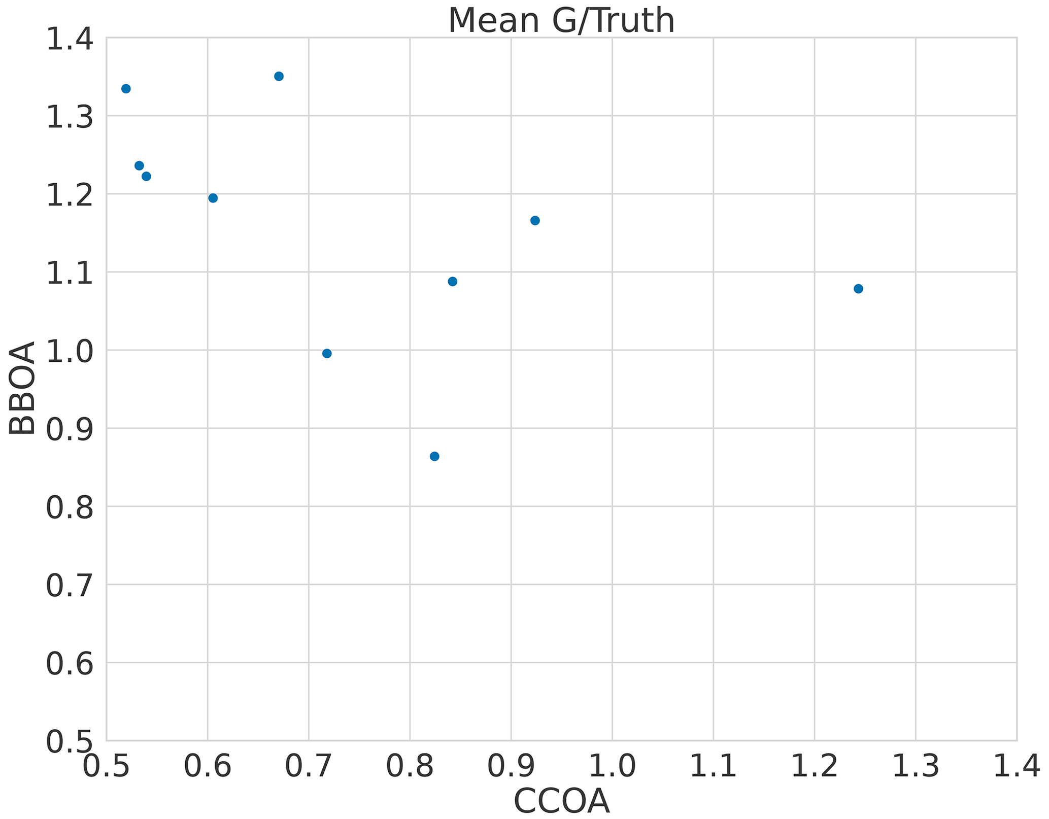
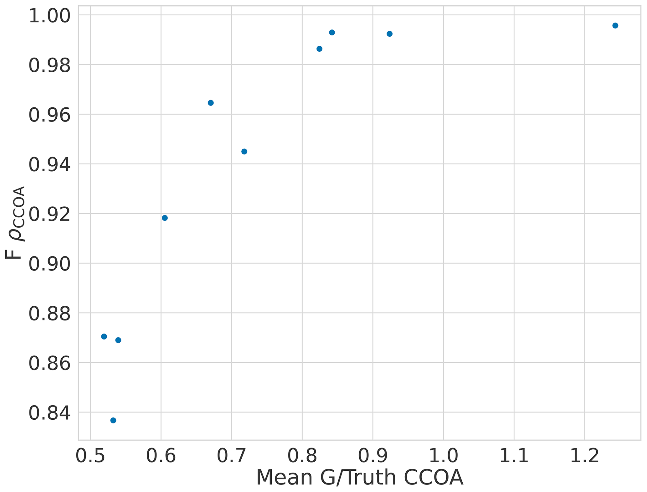
Figure A2The bias of CCOA time series and composition in the five-component megacity datasets.
Comparing the true components of the datasets shows that the European dataset components are much more correlated both in G Tables B1 and B3, as well as F Tables B2 and B4. Overall F components have similar, very high, correlations with each other, while the G components are markedly more correlated with each other in the European dataset than in the megacity datasets, with biological SOA being the exception.
Table B1Pearson correlation and standard deviation of the G components used to construct the 10 five-component megacity datasets.
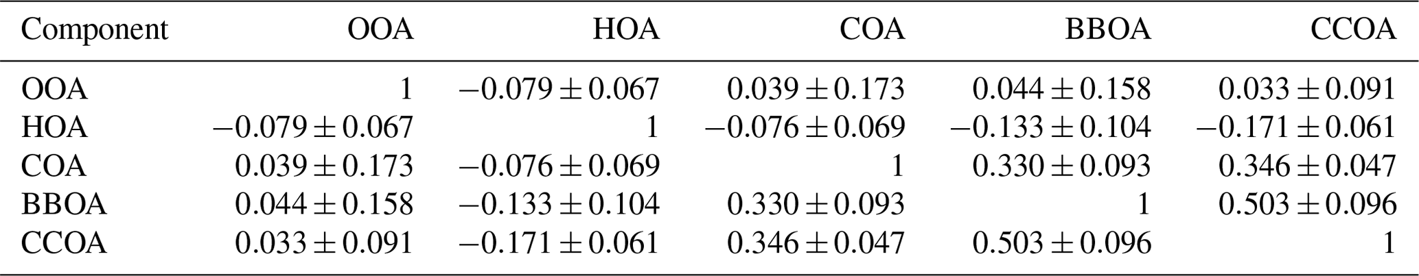
Table B2Spearman correlation of the F components used to construct the five-component megacity datasets. Note that F does not change between datasets, and thus standard deviation is 0.
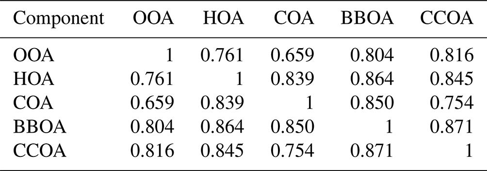
Table B3Pearson correlation of the G components used to construct the European dataset.
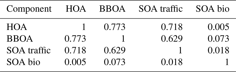
Table B4Spearman correlation of the F components used to construct the European dataset.
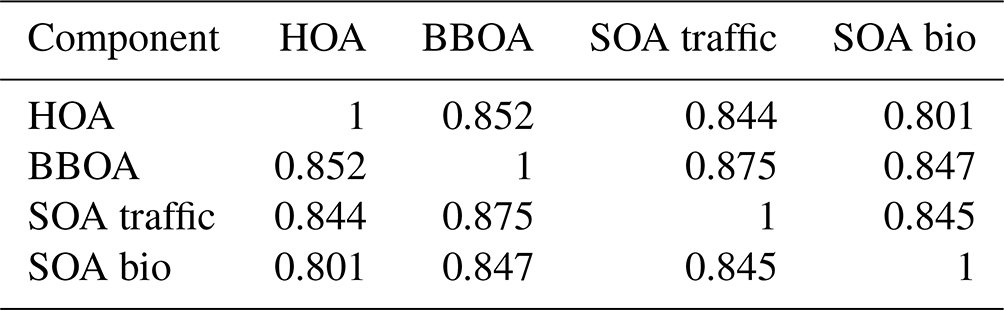
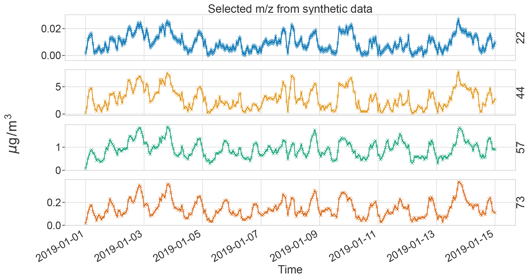
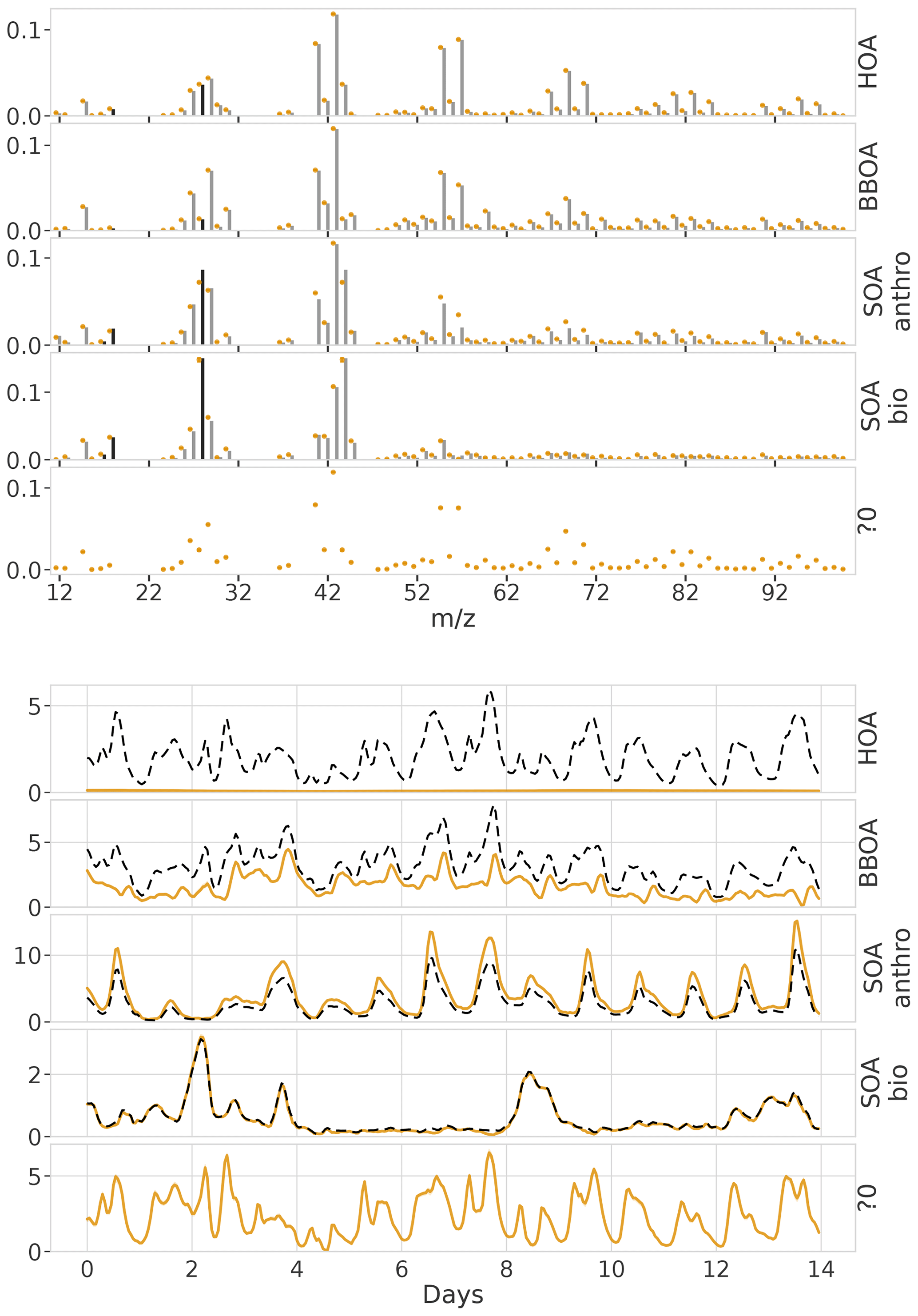
Figure E1 summarizes the steps used to run the BAMF model in this study and their order. In this study the profiles were from the literature (see Appendix F). In general use, the data generation step is not needed.
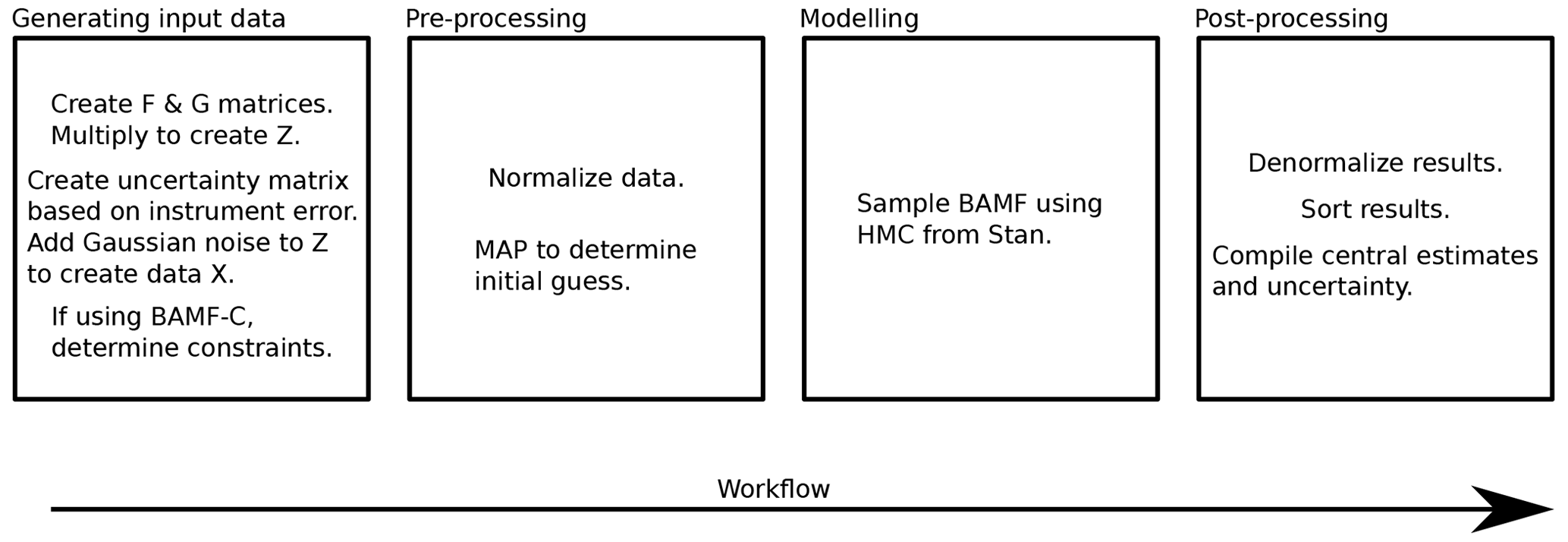
Figure E1Workflow of running the BAMF model in this study. Pre- and post-processing steps are technically optional but help in the convergence and interpretation of the results. With PMF the pre-processing and denormalization are skipped and the modeling box is just PMF, but we still sort the data similarly.
Table F1 summarizes the source profiles and constraints used. Constraints were only applied in the European dataset.
Elser et al. (2016)Elser et al. (2016)Elser et al. (2016)Elser et al. (2016)Elser et al. (2016)Elser et al. (2016)Elser et al. (2016)Daellenbach et al. (2017)Sage et al. (2008)Table F1The source profiles used to construct the datasets. The profiles were restricted to 12–100, summed to unit mass intervals, and normalized to sum to 1.
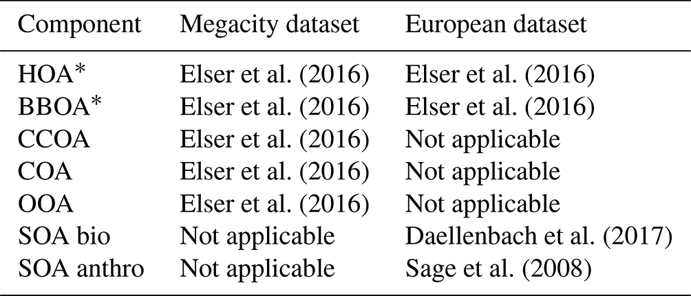
* Indicates the values from this profile were also used as constraints.
Figure G1 compares PMF with constraints to BAMF without them. This represents the absolute best-case scenario for PMF where you know the exact HOA and BBOA profiles beforehand. As mentioned in the main text, this does not fix the inability to resolve SOA bio.
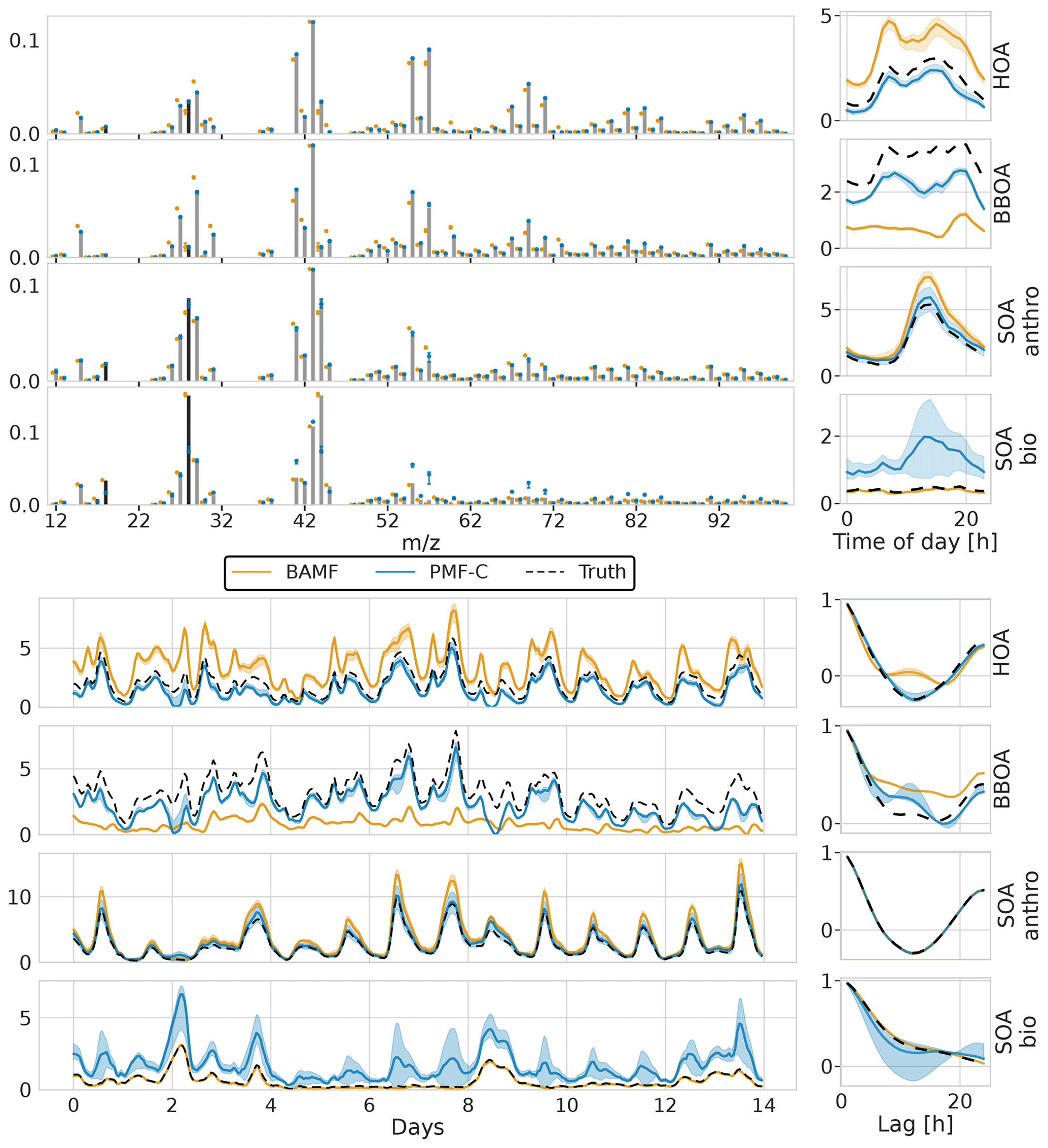
Figure G1Unconstrained BAMF and constrained PMF on the European dataset with four components.
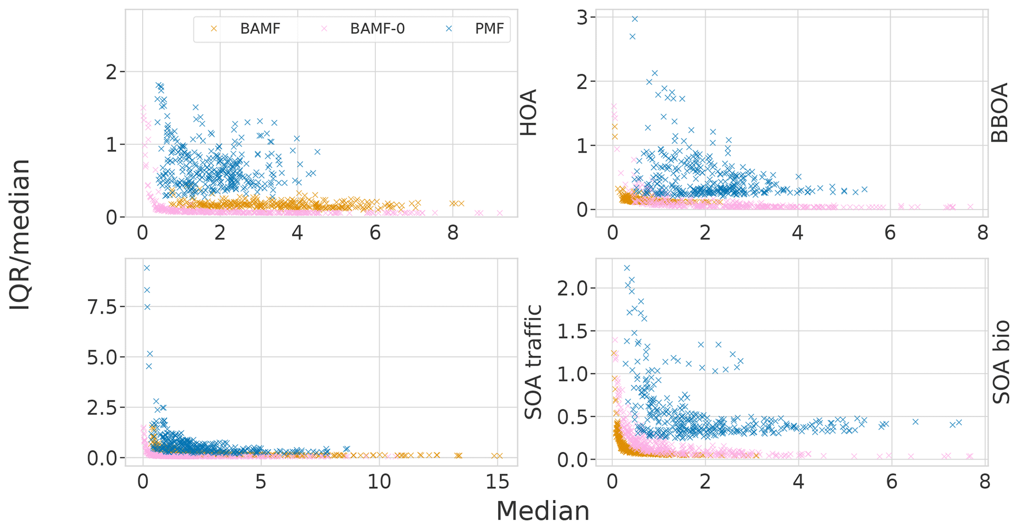
The error bars and the shaded areas in the time series are based on the interquartile ranges (IQR) in the empirical distribution given by the MCMC sampler. This gives us an idea of how accurately we can fix the modeled concentrations and compositions. In these results the error estimation is a bit optimistic, since it does not always cover the true solution. The underestimation is possibly due to the strictness of IQR and it not considering the model choice error. Figure H1 shows how the IQR compares to the median answer, with small concentrations having the most relative uncertainty. It also shows that BAMF-0 and PMF are often more uncertain than BAMF. In the case of PMF this is probably due to the values not being samples but solutions with different random seeds.
The datasets are available at https://doi.org/10.5281/zenodo.10629577 (Rusanen et al., 2024a) and the software at https://doi.org/10.5281/zenodo.10629849 (Rusanen et al., 2024b).
AR, AB, KRD, and KP participated in the model, dataset, and experiment development. AR ran and analyzed the experiments. KRD and MIM contributed to the PMF model solutions. JJ did the transport model runs. KRD, KP and MTK supervised the work. All authors contributed to the writing of the manuscript.
The contact author has declared that none of the authors has any competing interests.
Publisher’s note: Copernicus Publications remains neutral with regard to jurisdictional claims made in the text, published maps, institutional affiliations, or any other geographical representation in this paper. While Copernicus Publications makes every effort to include appropriate place names, the final responsibility lies with the authors.
We thank the Research Council of Finland for its support. Kaspar R. Daellenbach acknowledges support by SNSF Ambizione. Jianhui Jiang acknowledges support by Science and Technology Commission of Shanghai Municipality, China.
This research has been supported by the Research Council of Finland (decision nos. 337549, 345704, and 346376). Kaspar R. Daellenbach has been supported by SNSF Ambizione (grant no. PZPGP2_201992). Jianhui Jiang has been supported by Science and Technology Commission of Shanghai Municipality, China (Shanghai Pujiang Program, grant no. 21PJ1402800).
Open-access funding was provided by the Helsinki University Library.
This paper was edited by Eric C. Apel and reviewed by two anonymous referees.
Allan, J. D., Jimenez, J. L., Williams, P. I., Alfarra, M. R., Bower, K. N., Jayne, J. T., Coe, H., and Worsnop, D. R.: Quantitative sampling using an Aerodyne aerosol mass spectrometer 1. Techniques of data interpretation and error analysis, J. Geophys. Res.-Atmos., 108, 4090, https://doi.org/10.1029/2002JD002358, 2003. a
Bates, J. T., Fang, T., Verma, V., Zeng, L., Weber, R. J., Tolbert, P. E., Abrams, J. Y., Sarnat, S. E., Klein, M., Mulholland, J. A., and Russell, A. G.: Review of Acellular Assays of Ambient Particulate Matter Oxidative Potential: Methods and Relationships with Composition, Sources, and Health Effects, Environ. Sci. Technol., 53, 4003–4019, https://doi.org/10.1021/acs.est.8b03430, 2019. a
Canagaratna, M., Jayne, J., Jimenez, J., Allan, J., Alfarra, M., Zhang, Q., Onasch, T., Drewnick, F., Coe, H., Middlebrook, A., Delia, A., Williams, L., Trimborn, A., Northway, M., DeCarlo, P., Kolb, C., Davidovits, P., and Worsnop, D.: Chemical and microphysical characterization of ambient aerosols with the aerodyne aerosol mass spectrometer, Mass Spectrom. Rev., 26, 185–222, 2007. a
Canonaco, F., Crippa, M., Slowik, J. G., Baltensperger, U., and Prévôt, A. S. H.: SoFi, an IGOR-based interface for the efficient use of the generalized multilinear engine (ME-2) for the source apportionment: ME-2 application to aerosol mass spectrometer data, Atmos. Meas. Tech., 6, 3649–3661, https://doi.org/10.5194/amt-6-3649-2013, 2013. a, b, c, d, e, f, g, h, i
Canonaco, F., Tobler, A., Chen, G., Sosedova, Y., Slowik, J. G., Bozzetti, C., Daellenbach, K. R., El Haddad, I., Crippa, M., Huang, R.-J., Furger, M., Baltensperger, U., and Prévôt, A. S. H.: A new method for long-term source apportionment with time-dependent factor profiles and uncertainty assessment using SoFi Pro: application to 1 year of organic aerosol data, Atmos. Meas. Tech., 14, 923–943, https://doi.org/10.5194/amt-14-923-2021, 2021. a, b
Carpenter, B., Gelman, A., Hoffman, M., Lee, D., Goodrich, B., Betancourt, M., Brubaker, M., Guo, J., Li, P., and Riddell, A.: Stan: A Probabilistic Programming Language, J. Stat. Softw., 76, 1–32, https://doi.org/10.18637/jss.v076.i01, 2017. a, b, c, d, e
Chazeau, B., El Haddad, I., Canonaco, F., Temime-Roussel, B., D'Anna, B., Gille, G., Mesbah, B., Prévôt, A. S., Wortham, H., and Marchand, N.: Organic aerosol source apportionment by using rolling positive matrix factorization: Application to a Mediterranean coastal city, Atmospheric Environment: X, 14, 100176, https://doi.org/10.1016/j.aeaoa.2022.100176, 2022. a
Chen, G.: European Aerosol Phenomenology - 8: Harmonised Source Apportionment of Organic Aerosol using 22 Year-long ACSM/AMS Datasets, Version 2nd, Zenodo [data set], https://doi.org/10.5281/zenodo.6672710, 2022. a
Chen, G., Canonaco, F., Tobler, A., Aas, W., Alastuey, A., Allan, J., Atabakhsh, S., Aurela, M., Baltensperger, U., Bougiatioti, A., De Brito, J. F., Ceburnis, D., Chazeau, B., Chebaicheb, H., Daellenbach, K. R., Ehn, M., El Haddad, I., Eleftheriadis, K., Favez, O., Flentje, H., Font, A., Fossum, K., Freney, E., Gini, M., Green, D. C., Heikkinen, L., Herrmann, H., Kalogridis, A.-C., Keernik, H., Lhotka, R., Lin, C., Lunder, C., Maasikmets, M., Manousakas, M. I., Marchand, N., Marin, C., Marmureanu, L., Mihalopoulos, N., Močnik, G., Nęcki, J., O'Dowd, C., Ovadnevaite, J., Peter, T., Petit, J.-E., Pikridas, M., Matthew Platt, S., Pokorná, P., Poulain, L., Priestman, M., Riffault, V., Rinaldi, M., Różański, K., Schwarz, J., Sciare, J., Simon, L., Skiba, A., Slowik, J. G., Sosedova, Y., Stavroulas, I., Styszko, K., Teinemaa, E., Timonen, H., Tremper, A., Vasilescu, J., Via, M., Vodička, P., Wiedensohler, A., Zografou, O., Cruz Minguillón, M., and Prévôt, A. S.: European aerosol phenomenology - 8: Harmonised source apportionment of organic aerosol using 22 Year-long ACSM/AMS datasets, Environ. Int., 166, 107325, https://doi.org/10.1016/j.envint.2022.107325, 2022. a
Crippa, M., DeCarlo, P. F., Slowik, J. G., Mohr, C., Heringa, M. F., Chirico, R., Poulain, L., Freutel, F., Sciare, J., Cozic, J., Di Marco, C. F., Elsasser, M., Nicolas, J. B., Marchand, N., Abidi, E., Wiedensohler, A., Drewnick, F., Schneider, J., Borrmann, S., Nemitz, E., Zimmermann, R., Jaffrezo, J.-L., Prévôt, A. S. H., and Baltensperger, U.: Wintertime aerosol chemical composition and source apportionment of the organic fraction in the metropolitan area of Paris, Atmos. Chem. Phys., 13, 961–981, https://doi.org/10.5194/acp-13-961-2013, 2013. a
Crippa, M., Canonaco, F., Lanz, V. A., Äijälä, M., Allan, J. D., Carbone, S., Capes, G., Ceburnis, D., Dall'Osto, M., Day, D. A., DeCarlo, P. F., Ehn, M., Eriksson, A., Freney, E., Hildebrandt Ruiz, L., Hillamo, R., Jimenez, J. L., Junninen, H., Kiendler-Scharr, A., Kortelainen, A.-M., Kulmala, M., Laaksonen, A., Mensah, A. A., Mohr, C., Nemitz, E., O'Dowd, C., Ovadnevaite, J., Pandis, S. N., Petäjä, T., Poulain, L., Saarikoski, S., Sellegri, K., Swietlicki, E., Tiitta, P., Worsnop, D. R., Baltensperger, U., and Prévôt, A. S. H.: Organic aerosol components derived from 25 AMS data sets across Europe using a consistent ME-2 based source apportionment approach, Atmos. Chem. Phys., 14, 6159–6176, https://doi.org/10.5194/acp-14-6159-2014, 2014. a
Daellenbach, K. R., Stefenelli, G., Bozzetti, C., Vlachou, A., Fermo, P., Gonzalez, R., Piazzalunga, A., Colombi, C., Canonaco, F., Hueglin, C., Kasper-Giebl, A., Jaffrezo, J.-L., Bianchi, F., Slowik, J. G., Baltensperger, U., El-Haddad, I., and Prévôt, A. S. H.: Long-term chemical analysis and organic aerosol source apportionment at nine sites in central Europe: source identification and uncertainty assessment, Atmos. Chem. Phys., 17, 13265–13282, https://doi.org/10.5194/acp-17-13265-2017, 2017. a, b, c, d
Daellenbach, K. R., Uzu, G., Jiang, J., Cassagnes, L.-E., Leni, Z., Vlachou, A., Stefenelli, G., Canonaco, F., Weber, S., Segers, A., Kuenen, J. J. P., Schaap, M., Favez, O., Albinet, A., Aksoyoglu, S., Dommen, J., Baltensperger, U., Geiser, M., El Haddad, I., Jaffrezo, J.-L., and Prévôt, A. S. H.: Sources of particulate-matter air pollution and its oxidative potential in Europe, Nature, 587, 414–419, 2020. a, b, c
Elser, M., Huang, R.-J., Wolf, R., Slowik, J. G., Wang, Q., Canonaco, F., Li, G., Bozzetti, C., Daellenbach, K. R., Huang, Y., Zhang, R., Li, Z., Cao, J., Baltensperger, U., El-Haddad, I., and Prévôt, A. S. H.: New insights into PM2.5 chemical composition and sources in two major cities in China during extreme haze events using aerosol mass spectrometry, Atmos. Chem. Phys., 16, 3207–3225, https://doi.org/10.5194/acp-16-3207-2016, 2016. a, b, c, d, e, f, g, h, i
Fröhlich, R., Cubison, M. J., Slowik, J. G., Bukowiecki, N., Prévôt, A. S. H., Baltensperger, U., Schneider, J., Kimmel, J. R., Gonin, M., Rohner, U., Worsnop, D. R., and Jayne, J. T.: The ToF-ACSM: a portable aerosol chemical speciation monitor with TOFMS detection, Atmos. Meas. Tech., 6, 3225–3241, https://doi.org/10.5194/amt-6-3225-2013, 2013. a, b
Gelman, A., Carlin, J. B., Stern, H. S., Dunson, D. B., Vehtari, A., and Rubin, D. B.: Bayesian data analysis, 3rd edn., CRC Press, ISBN 9781439898208, 2014. a, b
Heikkinen, L., Äijälä, M., Daellenbach, K. R., Chen, G., Garmash, O., Aliaga, D., Graeffe, F., Räty, M., Luoma, K., Aalto, P., Kulmala, M., Petäjä, T., Worsnop, D., and Ehn, M.: Eight years of sub-micrometre organic aerosol composition data from the boreal forest characterized using a machine-learning approach, Atmos. Chem. Phys., 21, 10081–10109, https://doi.org/10.5194/acp-21-10081-2021, 2021. a
Hirtzel, C., Corotis, R., and Quon, J.: Estimating the maximum value of autocorrelated air quality measurements, Atmospheric Environment (1967), 16, 2603–2608, 1982. a
Hoffman, M. D. and Gelman, A.: The No-U-Turn sampler: adaptively setting path lengths in Hamiltonian Monte Carlo, J. Mach. Learn. Res., 15, 1593–1623, 2014. a
Hopke, P. K.: Review of receptor modeling methods for source apportionment, J. Air Waste Manage., 66, 237–259, https://doi.org/10.1080/10962247.2016.1140693, 2016. a
Huang, R.-J., Wang, Y., Cao, J., Lin, C., Duan, J., Chen, Q., Li, Y., Gu, Y., Yan, J., Xu, W., Fröhlich, R., Canonaco, F., Bozzetti, C., Ovadnevaite, J., Ceburnis, D., Canagaratna, M. R., Jayne, J., Worsnop, D. R., El-Haddad, I., Prévôt, A. S. H., and O'Dowd, C. D.: Primary emissions versus secondary formation of fine particulate matter in the most polluted city (Shijiazhuang) in North China, Atmos. Chem. Phys., 19, 2283–2298, https://doi.org/10.5194/acp-19-2283-2019, 2019. a
IPCC (Intergovernmental Panel on Climate Change): Climate Change 2021 – The Physical Science Basis: Working Group I Contribution to the Sixth Assessment Report of the Intergovernmental Panel on Climate Change, Cambridge University Press, Cambridge, https://doi.org/10.1017/9781009157896, 2023. a
Isokääntä, S., Kari, E., Buchholz, A., Hao, L., Schobesberger, S., Virtanen, A., and Mikkonen, S.: Comparison of dimension reduction techniques in the analysis of mass spectrometry data, Atmos. Meas. Tech., 13, 2995–3022, https://doi.org/10.5194/amt-13-2995-2020, 2020. a, b
Jiang, J., Aksoyoglu, S., El-Haddad, I., Ciarelli, G., Denier van der Gon, H. A. C., Canonaco, F., Gilardoni, S., Paglione, M., Minguillón, M. C., Favez, O., Zhang, Y., Marchand, N., Hao, L., Virtanen, A., Florou, K., O'Dowd, C., Ovadnevaite, J., Baltensperger, U., and Prévôt, A. S. H.: Sources of organic aerosols in Europe: a modeling study using CAMx with modified volatility basis set scheme, Atmos. Chem. Phys., 19, 15247–15270, https://doi.org/10.5194/acp-19-15247-2019, 2019. a, b
Kuhn, H. W.: The Hungarian method for the assignment problem, Naval Res. Logist. Q., 2, 83–97, 1955. a, b
Kulmala, M., Dada, L., Daellenbach, K. R., Yan, C., Stolzenburg, D., Kontkanen, J., Ezhova, E., Hakala, S., Tuovinen, S., Kokkonen, T. V., Kurppa, M., Cai, R., Zhou, Y., Yin, R., Baalbaki, R., Chan, T., Chu, B., Deng, C., Fu, Y., Ge, M., He, H., Heikkinen, L., Junninen, H., Liu, Y., Lu, Y., Nie, W., Rusanen, A., Vakkari, V., Wang, Y., Yang, G., Yao, L., Zheng, J., Kujansuu, J., Kangasluoma, J., Petäjä, T., Paasonen, P., Järvi, L., Worsnop, D., Ding, A., Liu, Y., Wang, L., Jiang, J., Bianchi, F., and Kerminen, V.-M.: Is reducing new particle formation a plausible solution to mitigate particulate air pollution in Beijing and other Chinese megacities?, Faraday Discuss., 226, 334–347, 2021. a, b
Lelieveld, J., Evans, J. S., Fnais, M., Giannadaki, D., and Pozzer, A.: The contribution of outdoor air pollution sources to premature mortality on a global scale, Nature, 525, 367–371, 2015. a
Liu, D. C. and Nocedal, J.: On the Limited Memory BFGS Method for Large Scale Optimization, Math. Program., 45, 503–528, https://doi.org/10.1007/BF01589116, 1989. a
Ng, N. L., Herndon, S. C., Trimborn, A., Canagaratna, M. R., Croteau, P. L., Onasch, T. B., Sueper, D., Worsnop, D. R., Zhang, Q., Sun, Y. L., and Jayne, J. T.: An Aerosol Chemical Speciation Monitor (ACSM) for Routine Monitoring of the Composition and Mass Concentrations of Ambient Aerosol, Aerosol Sci. Tech., 45, 780–794, 2011. a
Paatero, P. and Tapper, U.: Positive matrix factorization: A non-negative factor model with optimal utilization of error estimates of data values, Environmetrics, 5, 111–126, 1994. a, b, c
Reyes-Villegas, E., Green, D. C., Priestman, M., Canonaco, F., Coe, H., Reyes-Villegas, E., Green, D. C., Priestman, M., Canonaco, F., Coe, H., Prévôt, A. S. H., and Allan, J. D.: Organic aerosol source apportionment in London 2013 with ME-2: exploring the solution space with annual and seasonal analysis, Atmos. Chem. Phys., 16, 15545–15559, https://doi.org/10.5194/acp-16-15545-2016, 2016. a
Rusanen, A., Björklund, A., Manousakas, M. I., Jiang, J., Kulmala, M. T., Puolamäki, K., and Daellenbach, K. R.: Bayesian auto-correlated matrix factorization, datasets, Version 1.0.0, Zenodo [data set], https://doi.org/10.5281/zenodo.10629577, 2024a. a
Rusanen, A., Björklund, A., Manousakas, M. I., Jiang, J., Kulmala, M. T., Puolamäki, K., and Daellenbach, K. R.: Bayesian auto-correlated matrix factorization, software, Version 1.0.0, Zenodo [code], https://doi.org/10.5281/zenodo.10629849, 2024b. a
Sage, A. M., Weitkamp, E. A., Robinson, A. L., and Donahue, N. M.: Evolving mass spectra of the oxidized component of organic aerosol: results from aerosol mass spectrometer analyses of aged diesel emissions, Atmos. Chem. Phys., 8, 1139–1152, https://doi.org/10.5194/acp-8-1139-2008, 2008. a, b
Schlag, P., Rubach, F., Mentel, T. F., Reimer, D., Canonaco, F., Henzing, J. S., Moerman, M., Otjes, R., Prévôt, A. S. H., Rohrer, F., Rosati, B., Tillmann, R., Weingartner, E., and Kiendler-Scharr, A.: Ambient and laboratory observations of organic ammonium salts in PM1, Faraday Discuss., 200, 331–351, 2017. a
Ulbrich, I., Handschy, A., Lechner, M., and Jimenez, J.: AMS Spectral Database, http://cires.colorado.edu/jimenez-group/AMSsd/ (last access: 25 April 2022), 2022. a, b, c, d
Ulbrich, I. M., Canagaratna, M. R., Zhang, Q., Worsnop, D. R., and Jimenez, J. L.: Interpretation of organic components from Positive Matrix Factorization of aerosol mass spectrometric data, Atmos. Chem. Phys., 9, 2891–2918, https://doi.org/10.5194/acp-9-2891-2009, 2009. a, b, c, d, e, f
Wang, Y.-X. and Zhang, Y.-J.: Nonnegative matrix factorization: A comprehensive review, IEEE T. Knowl. Data En., 25, 1336–1353, 2012. a, b
Watson, J. G., Chow, J. C., and Fujita, E. M.: Review of volatile organic compound source apportionment by chemical mass balance, Atmos. Environ., 35, 1567–1584, https://doi.org/10.1016/S1352-2310(00)00461-1, 2001. a
Zhang, J., Li, R., Zhang, X., Bai, Y., Cao, P., and Hua, P.: Vehicular contribution of PAHs in size dependent road dust: A source apportionment by PCA-MLR, PMF, and Unmix receptor models, Science Total Environ., 649, 1314–1322, 2019. a
Zhang, Q., Jimenez, J. L., Canagaratna, M. R., Allan, J. D., Coe, H., Ulbrich, I., Alfarra, M. R., Takami, A., Middlebrook, A. M., Sun, Y. L., Dzepina, K., Dunlea, E., Docherty, K., DeCarlo, P. F., Salcedo, D., Onasch, T., Jayne, J. T., Miyoshi, T., Shimono, A., Hatakeyama, S., Takegawa, N., Kondo, Y., Schneider, J., Drewnick, F., Borrmann, S., Weimer, S., Demerjian, K., Williams, P., Bower, K., Bahreini, R., Cottrell, L., Griffin, R. J., Rautiainen, J., Sun, J. Y., Zhang, Y. M., and Worsnop, D. R.: Ubiquity and dominance of oxygenated species in organic aerosols in anthropogenically-influenced Northern Hemisphere midlatitudes, Geophys. Res. Lett., 34, L13801, https://doi.org/10.1029/2007GL029979, 2007. a
Zhang, Q., Jimenez, J. L., Canagaratna, M. R., Ulbrich, I. M., Ng, N. L., Worsnop, D. R., and Sun, Y.: Understanding atmospheric organic aerosols via factor analysis of aerosol mass spectrometry: a review, Anal. Bioanal. Chem., 401, 3045–3067, 2011. a, b, c, d
Zhang, Y., Favez, O., Canonaco, F., Liu, D., Močnik, G., Amodeo, T., Sciare, J., Prévôt, A. S. H., Gros, V., and Albinet, A.: Evidence of major secondary organic aerosol contribution to lensing effect black carbon absorption enhancement, npj Climate and Atmospheric Science, 1, 47, https://doi.org/10.1038/s41612-018-0056-2, 2018. a
Zhu, Q., Huang, X.-F., Cao, L.-M., Wei, L.-T., Zhang, B., He, L.-Y., Elser, M., Canonaco, F., Slowik, J. G., Bozzetti, C., El-Haddad, I., and Prévôt, A. S. H.: Improved source apportionment of organic aerosols in complex urban air pollution using the multilinear engine (ME-2), Atmos. Meas. Tech., 11, 1049–1060, https://doi.org/10.5194/amt-11-1049-2018, 2018. a
- Abstract
- Introduction
- Methods
- Datasets
- Results and discussion
- Conclusions
- Appendix A: The correlation of BAMF CCOA error in the five-component megacity datasets
- Appendix B: Correlation between true components in the datasets
- Appendix C: Concentration and uncertainty at selected zs for synthetic megacity ToF-ACSM OA data
- Appendix D: Overspecified BAMF-C results
- Appendix E: Workflow in this study
- Appendix F: Profiles and constraints used
- Appendix G: Comparison of constrained PMF and BAMF
- Appendix H: Error estimates and interquartile range
- Code and data availability
- Author contributions
- Competing interests
- Disclaimer
- Acknowledgements
- Financial support
- Review statement
- References