First validation of high-resolution satellite-derived methane emissions from an active gas leak in the UK

Atmospheric methane (CH₄) is the second-most-important anthropogenic greenhouse gas and has a 20-year global warming potential 82 times greater than carbon dioxide (CO₂). Anthropogenic sources account for ∼ 60 % of global CH₄ emissions, of which 20 % come from oil and gas exploration, production and distribution. High-resolution satellite-based imaging spectrometers are becoming important tools for detecting and monitoring CH₄ point source emissions, aiding mitigation. However, validation of these satellite measurements, such as those from the commercial GHGSat satellite constellation, has so far not been documented for active leaks. Here we present the monitoring and quantification, by GHGSat's satellites, of the CH₄ emissions from an active gas leak from a downstream natural gas distribution pipeline near Cheltenham, UK, in the spring and summer of 2023 and provide the first validation of the satellite-derived emission estimates using surface-based mobile greenhouse gas surveys. We also use a Lagrangian transport model, the UK Met Office's Numerical Atmospheric-dispersion Modelling Environment (NAME), to estimate the flux from both satellite- and ground-based observation methods and assess the leak's contribution to observed concentrations at a local tall tower site (30 km away). We find GHGSat's emission estimates to be in broad agreement with those made from the in situ measurements. During the study period (March–June 2023) GHGSat's emission estimates are 236–1357 kg CH₄ h⁻¹, whereas the mobile surface measurements are 634–846 kg CH₄ h⁻¹. The large variability is likely down to variations in flow through the pipe and engineering works across the 11-week period. Modelled flux estimates in NAME are 181–1243 kg CH₄ h⁻¹, which are lower than the satellite- and mobile-survey-derived fluxes but are within the uncertainty. After detecting the leak in March 2023, the local utility company was contacted, and the leak was fixed by mid-June 2023. Our results demonstrate that GHGSat's observations can produce flux estimates that broadly agree with surface-based mobile measurements. Validating the accuracy of the information provided by targeted, high-resolution satellite monitoring shows how it can play an important role in identifying emission sources, including unplanned fugitive releases that are inherently challenging to identify, track, and estimate their impact and duration. Rapid, widespread access to such data to inform local action to address fugitive emission sources across the oil and gas supply chain could play a significant role in reducing anthropogenic contributions to climate change.

1 Introduction

Atmospheric methane (CH₄) has a 20-year global warming potential 82 times greater than carbon dioxide (CO₂), and the increase in atmospheric CH₄ concentrations since 1750 has contributed an extra 23 % to the radiative forcing in the troposphere (Forster et al., 2021; Saunois et al., 2020). CH₄ has a mixture of natural and anthropogenic sources. Anthropogenic sources account for ∼ 60 % of global CH₄ emissions, of which 20 % come from oil and gas exploitation and transportation (Saunois et al., 2020). The United Kingdom (UK) contributes 0.48 % (EDGAR, 2022) to global anthropogenic CH₄ emissions and 9 % of UK anthropogenic emissions are from fugitive emissions from fuels (NAEI, 2023). Fugitive emissions of CH₄ from oil and gas distribution in the UK were estimated to be 187.3 kt of CH₄ in 2020 (NAEI, 2023). Natural gas is mostly composed of CH₄ (Bains et al., 2016), and fugitive emissions are unintentional releases of substances, such as natural gas, making them difficult to estimate.

In the UK, fugitive emissions of natural gas from low-pressure distribution, medium-pressure gas mains and above-ground installations are currently estimated by individual utility companies using the industry-wide Shrinkage and Leakage Model (SLM). The model combines parameters including pipeline length, annual leakage rate and average system pressure correction to estimate fugitive emissions, which are then aggregated to give a UK estimate (Marshall, 2023). The leakage rates are determined by sampling pipes during National Leakage Tests commissioned by the UK gas distribution networks (GDNs; Gas Governance, 2020). However, regular monitoring of pipes and detection of leaks through other methods, such as emission identification and source rate quantification from high-resolution satellite observations and in situ monitoring, could be incorporated into leakage estimates to improve frequency of quantification and validate estimates.

The UK currently does not have a system to regularly monitor fugitive emissions of CH₄, but the United Nations Environment Programme (UNEP) International Methane Emissions Observatory (IMEO) has a Methane Alert and Response System (MARS; United Nations Environment Programmes, 2023) to inform governments and organisations of large emissions. MARS uses the TROPOspheric Monitoring Instrument (TROPOMI) on board Sentinel-5P to identify very large methane plumes (> 25 000 kg h⁻¹, Lauvaux et al., 2022) and other very large methane hot spots and combines other satellite instruments such as the Italian Space Agency's Hyperspectral Precursor of the Application Mission (ASI PRISMA) to attribute the plume to a specific source. TROPOMI has a pixel size of 5.5 km × 7 km with a detection threshold of 25 000 kg h⁻¹ (Lauvaux et al., 2022) and ASI PRISMA 30 m × 30 m with a detection threshold of 500–2000 kg h⁻¹ (Guanter et al., 2021). MARS is an example of how high-resolution satellite-based imaging spectrometers, such as TROPOMI and ASI PRISMA, are becoming important tools for detecting and monitoring CH₄ point source emissions, aiding mitigation globally.

GHGSat was the first satellite constellation launched specifically for CH₄ point source emission identification, quantification and attribution and was the first system to provide high-resolution data to IMEO, although these data are not incorporated into MARS. GHGSat's constellation provides global monitoring of sites that are emitting above 100 kg h⁻¹ and also targets locations based on detected emissions using Sentinel-5P or Sentinel-2 (Schuit et al., 2023). Not all leaks can be detected by global monitoring satellites, such as Sentinel-5P or Sentinel-2, due to their high detection threshold and lower resolution, and so GHGSat's ability to detect smaller sources is important for observing leaks that might otherwise go undetected and unreported. However, there is a trade-off between global monitoring satellites and GHGSat because GHGSat requires a target to observe. GHGSat has previously detected and quantified CH₄ emissions from a variety of sources including landfill sites, coal mining and natural gas pipelines (GHGSat, 2022; ESA, 2021; GHGSat, 2023). Validation of GHGSat's technology has been performed on controlled releases and blind validation tests (McKeever and Jervis, 2022; Sherwin et al., 2023). There are a number of different methods that can be used to estimate emissions from point sources using measurements from satellite data, for example, Gaussian plume model, local mass balance for near-source pixels, Gauss's theorem, cross-sectional flux (CSF) and integrated mass enhancement (IME) (Jacob et al., 2016).

Validation of the emission estimates from the GHGSat satellite constellation, using the IME method, has so far not been documented for active leaks. Here we present the detection, monitoring and quantification, by GHGSat's satellites, of CH₄ emissions from an active gas leak near Cheltenham, UK, in the spring and summer of 2023 and provide the first study using surface-based mobile greenhouse gas surveys to validate GHGSat's estimates. There are two main methods for estimating the emission flux from surface-based mobile surveys, namely the Gaussian plume model and the Other Test Method 33A (OTM 33A).

In this study we provide estimates of the Cheltenham gas leak using three different methods: (i) GHGSat-derived fluxes using the IME method, (ii) fluxes derived from ground-based observations using a Gaussian plume model, and (iii) estimates from plumes simulated by the UK Met Office's Numerical Atmospheric-dispersion Modelling Environment (NAME, Jones et al., 2007) scaled to match the satellite and mobile survey observations. We also estimate mole fractions from the leak at a local tall tower monitoring site using NAME. We compare the modelled mole fractions from the gas leak with the observed above-background concentrations and discuss the implications of the leak in terms of the UK National Atmospheric Emissions Inventory (NAEI) and the success in monitoring and mitigating it. Note that, throughout this text, we refer to kg CH₄ h⁻¹ as kg h⁻¹.

2 Methods

2.1 Gas leak location

The University of Leeds requested, through the Third Party Missions (TPM) programme with the European Space Agency (ESA), that GHGSat monitor a landfill site near the town of Cheltenham, UK, and provide Level 4 emission estimate data. By chance, the monitored area included the location of a large (> 100 kg h⁻¹) gas leak (within 1 km of the landfill), allowing it to be detected by the satellite constellation. The landfill site was found to be below the satellite's detection threshold. The gas leak was first detected by GHGSat during its first cloud-free overpass on 27 March 2023, and the location of the leak from the satellite was estimated to be 51.95097° N, 2.09956° W at approximately 33 m above sea level (m a.s.l.). A GHGSat operator determines the source location by the shape of the observed plume (plume tail direction) and the area most concentrated at the beginning of the plume tail. When the plume boundaries and concentration gradient in the plume do not show a traditional directional plume shape, the wind direction from Goddard Earth Observing System Forward Processing (GEOS FP; NASA GMAO, 2023) is used to determine which side of the emission will most likely correspond to the source location. When GHGSat detects an emission from a site which is not in their database, other datasets such as visible satellite imagery and infrastructure maps are used to determine the source. In this case, GHGSat confirmed the source by contacting the utility company. The leak was from a low-pressure gas distribution pipeline situated in a field next to a railway line, approximately 5 km north of Cheltenham. The UK gas pipeline network is currently being upgraded from old metal pipes to new plastic ones, and it is likely that the gas leak came from an older pipe (Wales & West Utilities, 2023). The GHGSat satellite constellation monitored the site over approximately 11 weeks (six successful observations, one with no emissions detected) until the leaking pipe was repaired. The area surrounding the leak is a mixture of pastoral and arable agricultural land with one farm ∼ 70 m to the east of the site, two waste management sites less than half a kilometre to the south, and a small residential area less than 200 m to the east and south-east of the leak location. The farm closest to the site rears cattle, so they are also a likely source of CH₄ to the atmosphere along with manure produced by other animals, although these sources are much more diffuse. There is one single carriageway road to the south of the leak location, which passes within ∼ 30 m of the estimated location of the gas leak. The leak location estimated here is an approximate location of the surface emission and is not necessarily the precise location of the pipeline break. In our analysis, we use a mean location for the leak, 51.95088° N, 2.09962° W, estimated by the satellite. The individual estimated locations for each satellite observation can be found in the Supplement. The estimated locations were in close agreement with each other, within ±25 m, apart from one outlier.

2.2 Atmospheric methane measurements

2.2.1 GHGSat measurements

GHGSat is a constellation of nine SmallSats (∼ 15 kg) orbiting in low Earth orbit at altitudes ranging from 500–550 km which retrieve vertical column density of CH₄ and detect concentration enhancements above background from targeted industrial facilities globally. The satellite retrievals are collected using a wide-angle Fabry–Pérot (WAF–P) imaging spectrometer, which is a hyperspectral spectrometer operating in the shortwave infrared (SWIR) at 1630–1675 nm, where methane absorption lines can be resolved for each pixel in the 12 km × 12 km sensor field of view (Jervis et al., 2021). This sensor system achieves both high spatial and spectral resolution, enabling precise geolocation and low noise measurements. For the eight commercially operating satellites (GHGSat-C1 to C8), the system achieves a spatial resolution of 25 m and spectral resolution of 0.3 nm (Jacob et al., 2022), having the capability of a 1–2 d revisit time. This allows for precise attribution of CH₄ emission enhancements to sources with emission rates above 100 kg h⁻¹ (50 % probability of detection at wind speeds of 3 m s⁻¹). The performance of the system has been independently verified through controlled releases of CH₄ at known rates that were measured using the GHGSat system (Sherwin et al., 2023).

The raw images collected by the satellites are processed through GHGSat's proprietary toolchain and reviewed by experts at GHGSat. The surface reflectance and column-averaged concentration of CH₄ in parts per billion (ppb) are retrieved for each pixel by fitting a model of the instrument and atmosphere. These data are georeferenced using satellite's GPS outputs and Landsat 8 imagery with sub-pixel accuracy, achieving a geolocation accuracy of ∼ 25 m for the source location.

2.2.2 Mobile greenhouse gas observations

Royal Holloway, University of London's (RHUL) mobile greenhouse gas laboratory was used for ground-based verification of the leak location, source type and emission rate. The mobile laboratory includes the following suite of cavity-enhanced laser absorption spectrometers for the measurement of CH₄, CO₂ and ethane (C₂H₆) mole fractions and methane isotopes (δ¹³C-CH₄): Picarro G2311-f (10 Hz CH₄ and CO₂); LI-COR LI-7810 (1 Hz CH₄ and CO₂); LGR UMEA, i.e. Ultraportable Methane/Ethane Analyser (1 Hz CH₄ and C₂H₆); and Picarro G2210-i (1 Hz CH₄, CO₂, C₂H₆ and δ¹³C-CH₄). The instruments are powered using a 6 kW portable lithium power station (Goal Zero Yeti 6000X). Air is pumped to the instruments from inlets on the roof of a hybrid car, 1.8 m above ground level (a.g.l.). A sonic anemometer (Campbell CSAT3B 3-D) and GPS receiver are also installed on the roof of the vehicle. Another air inlet is connected to a diaphragm pump for filling 3 L multilayer foil bags with air, for subsequent high-precision methane δ¹³C analysis by isotope ratio mass spectrometry (Fisher et al., 2006) and methane mole fraction analysis using the LI-7810. The air bags were filled when the car was parked both in and outside of the emissions plume. Instruments are harmonised to international scales for CH₄ and CO₂ at RHUL using cylinders of ambient air calibrated by the NOAA (National Oceanic and Atmospheric Administration).

Mobile surveys were carried out during daytime on 26 May, 12 June and 22 June 2023. These dates were chosen because the wind direction was between NW and ENE, allowing the emissions plume to be measured on the nearest road, which was to the south of where GHGSat had identified the source. During each survey, the car was driven at 20–30 mph (32–48 km h⁻¹) on a public road downwind of the emissions site with at least 12 passes. The public road included a road bridge over a railway, close to the satellite-derived leak location.

2.2.3 Greenhouse gas tall tower measurements

The UK Deriving Emissions linked to Climate Change (UK DECC) network currently consists of four tall tower sites within the UK (in addition to the baseline station at Mace Head, Ireland). The UK DECC network has been collecting measurements since 2012 and measures various atmospheric constituents including CH₄ (Stanley et al., 2018). CH₄ is measured by a cavity ring-down spectrometer (CRDS) at multiple inlet heights. The CRDS is calibrated using both a standard of approximately ambient mole fraction and a set of calibration standards which range above and below ambient mole fractions (Stanley et al., 2018). Calibrant and standard gases are used in the CRDS at all sites and are of natural composition. The standard gas is measured once a day to assess linear instrumental drift, and the calibration gases are measured once a month to assess for instrument nonlinearity. The repeatability of the daily standard measurements is < 0.3 nmol mol⁻¹ (Stanley et al., 2018). The two key stations from the UK DECC network in this study are Mace Head (MHD) on the west coast of Ireland and Ridge Hill (RGL) in central-western England. MHD is at 53.32667° N, 9.90456° W and close to the shoreline. The surrounding area is sparsely populated, resulting in low local anthropogenic emissions at the site. Prevailing winds from the west and south-west bring well-mixed Atlantic air to MHD. As a result, the majority of measurements obtained at MHD at 10 m a.g.l. are representative of Northern Hemisphere, mid-latitude background concentrations (Stanley et al., 2018). RGL is a rural site situated at 51.99747° N, 2.53992° W which is approximately 30 km east of the border between England and Wales. RGL is surrounded by land primarily used for agriculture. It is also 16 km south-east from Hereford and 30 km south-west of Worcester, both large towns, and there are a number of wastewater treatment plants within a 40 km radius of the site (Stanley et al., 2018). RGL measures CH₄ at 45 and 90 m a.g.l. and in this study, we use measurements from the 90 m a.g.l. inlet because it has a larger footprint of influence. The different source sectors surrounding RGL have an impact on the observed concentrations, but the main waste sites in the area are not upwind of the leak, which is 30 km east of RGL.

We use the concentrations representative of well-mixed, mid-latitude, Northern Hemisphere air measured at MHD to produce a time-varying background concentration at RGL, as described in Manning et al. (2021). The background concentrations are subtracted from the observed concentrations to obtain an above-background concentration at RGL.

2.3 Flux estimation methods

2.3.1 GHGSat flux estimation

The satellite-derived fluxes are estimated using the integrated mass enhancement (IME) method (Varon et al., 2018). First, the emission signal is identified and masked by isolating methane enhancements that are not instrument artefacts or signals from albedo features. The IME method relates the emission source rate to the emission mass downwind of the source (defined by the masked methane concentration and the source location) based on the expected transport of methane in the wind (defined by the GEOS FP model wind data). The IME of the observed plume is

$$\begin{array}{}\text{(1)}& \text{IME}={\sum }_{j=\mathrm{1}}^N\mathrm{\Delta }{\mathrm{\Omega }}_j{A}_j,\left(j=\mathrm{1}\mathrm{\dots }N\right),\end{array}$$

where N is the number of pixels, ΔΩ_j is the mean source pixel enhancement and A_j is area of each pixel. The IME of the observed plume and the source rate Q are related by the residence time of methane in the plume, τ, where τ can be expressed in terms of the effective wind speed U_eff (m s⁻¹) and plume size L (m) as

$$\begin{array}{}\text{(2)}& Q={\displaystyle \frac{\text{IME}}{\mathit{\tau }}}={\displaystyle \frac{U_{\mathrm{eff}}}{L}}\text{IME}={\displaystyle \frac{U_{\mathrm{eff}}}{L}}{\sum }_{j=\mathrm{1}}^N\mathrm{\Delta }{\mathrm{\Omega }}_j{A}_j,\end{array}$$

where U_eff is a function of the 10 m wind speed from GEOS FP; see Varon et al. (2018) for the full description of the IME method. The uncertainty on the source rate is the 1σ standard deviation based on the uncertainties on the wind speed, measurement uncertainties and the IME model parameters, where the wind speed is the dominant source of uncertainty. Details of how the wind speed uncertainty is calculated can be found in the Supplement of Varon et al. (2019).

There are a number of different methods to estimate the flux using satellite data, as listed in Sect. 1. The Gaussian plume model is the simplest way to simulate a CH₄ plume and is described in Sect. 2.3.2. Due to atmospheric conditions, CH₄ plumes can be turbulent and sometimes discontinuous, which means that it can be unrealistic to model satellite-observed plumes as Gaussian (Jongaramrungruang et al., 2019). The local mass balance method for near-source pixels estimates the flux by only considering the column enhancement over the point source pixel, neglecting information of the plume downwind (Varon et al., 2018). This method can be effective when the pixel size is coarse and contains most of the information of the plume. However, it is not suitable for high-resolution retrievals, such as those from GHGSat, because it does not use information of the plume downwind, where there may be strong variability in the wind from small-scale turbulence, and the source pixel transport may be by turbulent horizontal diffusion rather than advection by the mean wind (Varon et al., 2018). The Gauss's theorem method is the outward flux summed along a contour surrounding the point source and does not account for the contribution of turbulent diffusion to the outward flux (Jacob et al., 2022). This method is often used for in situ aircraft observations which circle the source and measure wind and methane at the same time (Jacob et al., 2022).

The cross-sectional flux (CSF) and IME methods are both used to estimate fluxes of point sources from satellite retrievals because they provide consistent results (Varon et al., 2019). The CSF method estimates the flux from the product of the methane enhancement and the wind speed integrated across the plume width. Varon et al. (2018) found that the IME method performs best for GHGSat data and is the selected method for our analysis.

2.3.2 Gaussian plume inversion method

The flux estimates from the mobile greenhouse gas measurements were calculated using a Gaussian plume model to determine the mole fraction of a gas as a function of distance downwind of a point source (Seinfeld and Pandis, 2006). We use this model, developed by Pasquill and Smith (1983), to estimate the emission rate of the source using the concentrations observed downwind of the plume to scale an idealised Gaussian plume model. In the idealised model, the mole fraction at a point in the plume is a function of flux of the source (Q, kg h⁻¹), advective horizontal wind speed (u, m s⁻¹), the rate of dispersion and the distance from the source; see Eq. (3). The plume measured during each transect during the mobile survey was manually identified in the dataset and distance and angle to the emission source calculated. We used a mean of the source locations provided by the satellite retrievals as the source location in the model. We then took the observed concentration data and wind speed data to create the initial model plume using Eq. (3). On 26 May we used a mean wind speed observed by the vehicle's 10 Hz sonic anemometer for each transect, whereas on 12 June we used wind speed data, averaged to the nearest hour, from the Met Office UKV model due to the unavailability of the anemometer.

$$\begin{array}{}\text{(3)}& \begin{array}{rl}C\left(x,y,z\right)=& {\displaystyle \frac{Q}{\mathit{\pi }{\mathit{\sigma }}_y{\mathit{\sigma }}_{z}u}}\exp (-{\displaystyle \frac{y^{\mathrm{2}}}{\mathrm{2}{\mathit{\sigma }}_y^{\mathrm{2}}}})\\ & \left[\exp \right(-{\displaystyle \frac{(z-h{)}^{\mathrm{2}}}{\mathrm{2}{\mathit{\sigma }}_z^{\mathrm{2}}}})+\exp (-{\displaystyle \frac{(z+h{)}^{\mathrm{2}}}{\mathrm{2}{\mathit{\sigma }}_z^{\mathrm{2}}}}\left)\right],\end{array}\end{array}$$

where C (µg m⁻³) is the atmospheric concentration of methane at $(x,y,z)$, x is the distance downwind from the source (m), y is the distance crosswind (m), z is the height above ground level (m), Q is the source strength (kg h⁻¹), σ_y and σ_z are the diffusion coefficients in the crosswind and vertical directions respectively, u represents the horizontal time-averaged wind speed (m s⁻¹), and h is the height of the release (m). The dispersion coefficients of the plume (σ_y and σ_z) are approximated using Briggs' assumptions in the Pasquill–Gifford atmospheric stability classification. The coefficients σ_y and σ_z are given as functions of downwind distance x (m) and stability class. Equation (4) shows the general form of parametrisation of plume width parameters according to Briggs (1973).

$$\begin{array}{}\text{(4)}& {\mathit{\sigma }}_y={\displaystyle \frac{\mathit{\alpha }x}{\sqrt{\mathrm{1}+\mathit{\beta }x}}}\text{and}{\mathit{\sigma }}_x=\mathit{\alpha }x(\mathrm{1}+\mathit{\beta }x{)}^{\mathit{\gamma }}\end{array}$$

The observations are measured in parts per billion (ppb) and are scaled to µg m⁻³ at standard temperature and pressure (STP) conditions. To scale from the idealised plume to the measurements, the flux through a control surface of 1 m height and the width of the plume is determined using the measurement data (Eq. 5).

$$\begin{array}{}\text{(5)}& \sum (c_i\left[{\mathrm{CH}}_{\mathrm{4}}\right]\cdot \mathrm{\Delta }{x}_i\cdot \mathrm{\Delta }z),\end{array}$$

where c_i is the concentration at point i, Δx_i is the distance driven by the car at this point and Δz=1 m is the vertical extent of the control surface. The height of the control surface is allowed to vary between 2 and 7 m a.g.l to best match the height of the vehicle inlet above ground level when accounting for the effect of the bridge structure. The corresponding control surface flux is then calculated for the modelled plume and the ratio between the measured control surface flux and the modelled control surface flux used to scale the model to the measured plume.

There are several assumptions made when using the Gaussian plume model. We assume that the source is emitting at a constant rate, the CH₄ mass is conserved, and there are no additional sources or sinks during transport. We also assume that the wind speed and vertical eddy diffusivity are constant, the diffusion in the x direction and horizontal wind shear are negligible, and the molecular diffusion is negligible compared to turbulent diffusion. Local baseline CH₄ is taken as the second-percentile measurement over a 5 min moving average window as per other mobile campaigns. However, only measurements more than 1 ppm above baseline concentrations were used in the calculation of gas leak flux to conservatively ensure that the total is not enhanced by any small emissions from surrounding sources such as the farm or waste sites. The baseline was calculated using the methods described in Fernandez et al. (2022).

We performed a Monte Carlo simulation to determine the CH₄ emission estimates and the associated uncertainty for each surface-based mobile survey. The leak location is randomly assigned to any point within an approximate 10 m × 10 m box around the mean location of the leak (derived by the satellite observations). The box is bounded by the following coordinates: 51.9506799° N, 2.099682° W; 51.9506635° N, 2.0997039° W; 51.9506682° N, 2.0997021° W; and 51.9506718° N, 2.0997023° W. The wind speed for each individual plume is determined using the mean wind speed during the traverse. The wind speed for each plume also has a random uncertainty assigned with a mean of 1 m s⁻¹ and was allowed to vary according to a Gaussian distribution. The vehicle height varied during the traverse of the plume due to the presence of a road bridge over a railway line. To account for the difference between the ground height and inlet height, we allowed the simulation to vary randomly between 2.5 and 6.5 m, with 1 m intervals. We also selected the most appropriate atmospheric stability classification based on the average wind speed per each Monte Carlo run. The sky conditions did not vary significantly during the period of measurement on each day, resulting in the selection being based on wind speed only (see Table S2 in the Supplement for the stability classes and meteorological conditions). The Monte Carlo simulation was run 1000 times for each suite of transects.

There are two main methods for estimating the flux using a ground-based mobile survey, as described in Sect. 1. The OTM 33A requires measurements to be taken downwind of the source, perpendicular to the wind direction, in order to detect the plume centre line. Once the centre line has been found, the CH₄ concentrations and meteorological conditions are measured continuously for 20 min. The emissions are then quantified using a Gaussian plume model with three assumptions; the measurement inlet is at the height of release, measurements are taken directly downwind of the source and reflection from the ground is negligible from the source (Ražnjević et al., 2022). However, in this study it was not feasible to carry out the OTM 33A because we took observations on a public road and could not be static in the plume for the required time.

2.4 NAME dispersion modelling

We simulated the dispersion of the gas leak through a suite of experiments using the UK Met Office's Numerical Atmospheric-dispersion Modelling Environment (NAME, Jones et al., 2007). We use NAME to estimate the flux of the leak using the observed concentrations from both GHGSat and the mobile survey to provide some continuity between the two observation and flux estimation techniques. We also modelled the leak's mole fractions of CH₄ at the Ridge Hill (RGL) tall tower site (30 km away) and compared them to the observed above-background concentrations at RGL.

NAME is a Lagrangian dispersion model which simulates the transport and dispersion of chemical species through the atmosphere (Jones et al., 2007). The model is offline and for this study is driven by the Met Office's numerical weather prediction (NWP) meteorology from the high-resolution UKV model (Davies et al., 2005; Bush et al., 2023). The UKV meteorology has a horizontal resolution of 1.5 km × 1.5 km and 70 vertical levels over the UK with hourly temporal resolution. NAME follows individual theoretical particles during the simulation, and the number of particles within the user-defined grid determines the total mass output per grid cell for each time step. Model particles are advected by three-dimensional wind fields provided by the NWP model and are dispersed using random walk techniques which account for turbulent velocity structures in the atmosphere (Jones et al., 2007). NAME includes additional parametrisations for atmospheric processes which are unresolved in the NWP model, which influence the transport of pollutants, including deep convection, horizontal mesoscale motions and turbulence (Meneguz and Thomson, 2014; Webster et al., 2018). The output resolution of NAME is user-defined, allowing a suite of experiments to be performed at various resolutions. In our simulations we assume the chemical sinks of CH₄ to be negligible due to the short transport time to both the road near the leak site (∼ minutes, depending on wind direction) and to RGL (∼ 7–10 h, depending on wind direction) compared to the long atmospheric lifetime of CH₄ (∼ 9 years, Prather et al., 2012).

In the first experiment, we set up a high-resolution grid in NAME to estimate the magnitude of the flux from the concentrations observed by the satellite and mobile survey. We did this to provide a flux estimation for both observation methods, using the same model and meteorology to provide some continuity between the satellite- and mobile-survey-derived estimates. To estimate the flux using the satellite retrievals, we simulated the gas leak with a unit release (1 g s⁻¹), starting 1 h before the time of observation, and simulated the release for 3 h. The simulation was output with a horizontal resolution of 25 m × 25 m with a 500 m vertical resolution up to 1000 m a.g.l. and a 1-hourly time step. We selected the model time step closest to the observation time to do our analysis. We produced a pressure-weighted mean total column value from the two layers, where concentrations in the layer above 500 m were approximately 0 ppb. The modelled and observed plumes did not overlap well, so we defined certain criteria in the modelled plume to capture the modelled dispersion of CH₄ in a way that is comparable with the GHGSat plume. We defined the plume by removing concentrations lower than 1 % of the maximum value and limited the length of the modelled plume to match the observed length of GHGSat's plume. This method assumes that the CH₄ emitted in NAME has travelled at the same distance and speed as detected by GHGSat. We integrated the CH₄ over the total column concentrations in both the GHGSat plume and the defined area of the NAME plume to obtain a scaling factor for the NAME flux. We then used this scaling factor to estimate the flux of the gas leak using NAME. To test the robustness of our modelled flux estimate we also calculated fluxes using two other plume definitions, by removing values (1) lower than 1 % of the maximum value and (2) lower than 5 % of the maximum value, ignoring the plume length criteria in both cases. We then scaled the model using the integrated mass from these defined plumes to test the robustness of the flux estimation method. Apart from the release location and length of the plume, no other constraints from the observed satellite plume are applied to the modelled plume. The three different plume definitions are analogous to the threshold value used by GHGSat filter noise around the detected plume.

We applied a similar mass integration method to estimate the flux in NAME using the observations from the mobile survey. We simulated the gas leak with a unit release (1 g s⁻¹), starting 1 h before the peak observation time and simulated the release for 3 h. The model was output at a horizontal resolution of 10 m × 10 m with a single 4 m layer to capture the volume observed by the mobile survey. We selected three values centred on the maximum concentration in the model and mobile survey concentrations along the road that the survey was completed. In the model the selected values include the maximum value of the plume along the road and the two grid boxes either side of the maximum value. From the observations, we used the median concentrations calculated from the different observed transects during the mobile survey (see Sect. S4 in the Supplement) and then selected the maximum value and the observations taken immediately before and after the maximum value. These values are approximately 10 m apart. We integrated across the three peak values for the model and mobile survey in order to the scale the model and derived a modelled flux. We then calculated flux estimation uncertainties by taking the three grid boxes to the left and three grid boxes to the right of the peak value on the road and used the mass of these grid boxes to scale the model to the observed peak concentrations. Flowcharts showing the calculation processes of the three different flux estimation methods can be found in Sect. S3.

The second experiment involved estimating the leak's contribution to the observed above-background concentrations at the nearby tall tower (RGL) and assessing the likelihood of the leak contributing to most of the observed above-background concentration. We ran NAME with an output resolution of 2.5 km × 2.5 km with 40 m vertical resolution up to 120 m a.g.l. to capture the height of the observations at RGL. We used the five observed emission rates provided by GHGSat. We simulated the leak as a point source in NAME at 51.95088° N, 2.09962° W from 27 March to 13 June, with the emission rate being held constant at each derived emission rate from the date that the observation was made until the date of the next available observation (see Fig. 3a). We also simulated the upper- and lower-uncertainty emission rates from the satellite-derived fluxes (see Fig. 3a). The model produced a 1-hourly time series output at the RGL tall tower location at 80–120 m a.g.l. which we compared to the above-background observations. This simulation is called “NAME_spring”. Note that the prevailing wind at the leak site is west–south-west, but a north-easterly wind is needed for the emissions from the leak to be transported to RGL.

In the third experiment, we simulated the leak with the same model setup as NAME_spring but with two alternative constant flux rates and simulated an extra year before the date that the leak was discovered, giving a simulation time of approximately 1 year and 5 months (1 March 2022 to 13 June 2023). We simulated both the maximum flux derived by GHGSat and the maximum flux derived from the mobile survey separately. This simulation is called “NAME_long”. We selected this time period to cover a full year previous to the leak discovery, to assess the frequency of large contributions at RGL from a theoretical leak over a longer time period, including different seasons. It should be noted that the UK DECC network was set up to monitor long-term greenhouse gas concentrations across the UK and is not specifically designed to detect fugitive emissions like this gas leak. However, due to the location of the tall tower site relative to the gas leak in this case (within 30 km), it is reasonable to consider whether it might have been possible to use statistical analysis and inverse modelling techniques to recognise that the leak was ongoing without the use of GHGSat.

3 Results

3.1 Observations and flux comparisons

We first observed an enhancement over a field, which was later confirmed to be a gas leak, on 27 March 2023 via satellite when targeting the nearby landfill site. The satellite was centred on 51.9402° N, 2.0998° W with a 12 km × 12 km field of view. After detecting the leak, GHGSat continued to monitor the site with same field of view to quantify how much CH₄ was being released. Figure 1 shows the CH₄ plumes measured by the satellite between 27 March and 16 June 2023. The initial observation on 27 March produced a flux estimate from the leak of 236 ± 157 kg h⁻¹, and the peak observed leak rate occurred on 20 May with an estimated flux rate of 1375 ± 481 kg h⁻¹. The observations taken after 20 May show that the size and strength of the plume was decreasing, with the last observed emission on 7 June with an estimated flux rate of 290 ± 130 kg h⁻¹. The satellite-derived fluxes were estimated using the IME method. The next successful observation on 16 June shows no emissions above the 100 kg h⁻¹ detection threshold.

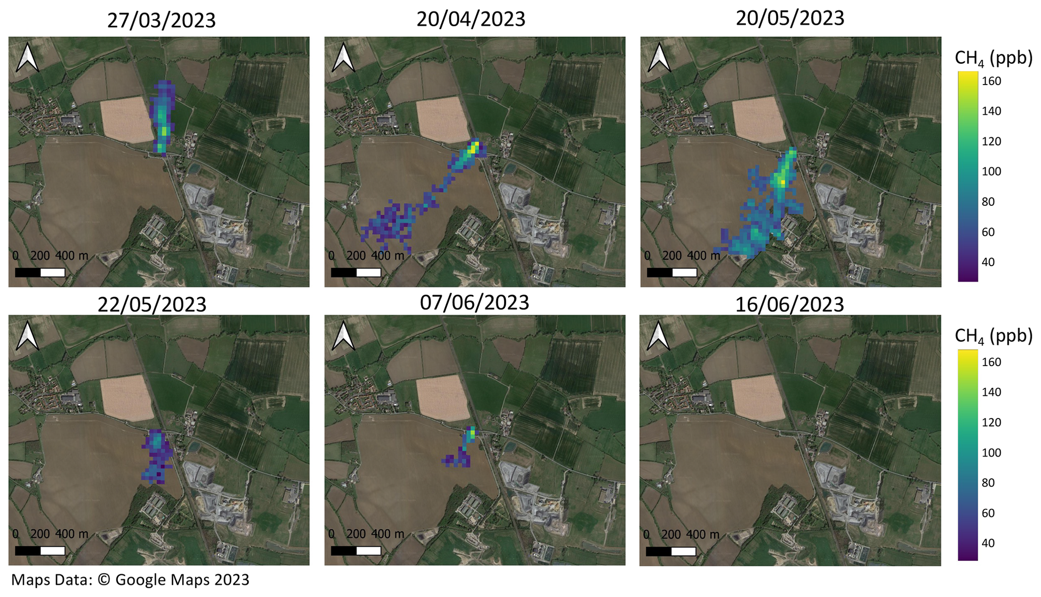
Figure 1 Total column CH₄ (ppb) observations from GHGSat showing the variation in strength and size of the plume from the gas leak on six dates between March and June 2023 (© Google Maps 2023). The geographical area shown is not the full field of view of the satellite and contains only the area where enhanced CH₄ concentrations were identified.

During the satellite observation period, we conducted mobile greenhouse gas surveys of the leak to validate the satellite measurements. On 26 May and 12 June, observed CH₄ mole fractions were large enough to be above the dynamic range (20 ppm but capable up to 60 ppm) of the Picarro G2311-f when driving through the plume. The LI-7810 data were therefore used for the Gaussian plume modelling. The maximum CH₄ mole fractions recorded in each pass were 77–588 ppm (77 000–588 000 ppb) on 26 May and 120–839 ppm (120 000–839 000 ppb) on 12 June. Gaussian plume estimates of the flux were estimated to be 846 ± 453 kg h⁻¹ on 26 May and 634 ± 299 kg h⁻¹ on 12 June. The ethane-to-methane ratio in the plume was 0.05, and the δ¹³C isotopic signature was −36.7 ± 2.1 ‰. These values are characteristic of the thermogenic gas in the UK gas network (Zazzeri et al., 2015; Lowry et al., 2020) and confirm that the leak was from a gas pipeline. On 22 June there were no significant enhanced concentrations recorded downwind of the leak site.

Figure 2 shows the timeline of events, including estimated fluxes (with their uncertainty), from both estimation methods. Also shown are the dates that the leak was reported to the utility company by GHGSat, when work started on the leak, when the leak was resolved according to the utility company, and when there were no further emissions detected by satellite or mobile surveys. Once the persistence of the leak was confirmed on 20 April, GHGSat contacted the utility company. A member of the public had also reported the smell of gas to the utility company prior to the notification from GHGSat, and the utility company started work on assessing and repairing the leak on 27 April. GHGSat continued to monitor the leak, and the validation of the satellite retrievals by mobile survey began on 22 May. We directly compare the flux estimates derived from the satellite and mobile surveys. Clouds obstructed the view of the satellite on the mobile survey days, so we compare the mobile-survey-derived fluxes with the most recent satellite-derived flux to validate the satellite fluxes. We compare the mobile-survey-derived flux on 26 May (846 ± 452 kg h⁻¹) and 12 June (634 ± 299 kg h⁻¹) with the satellite-derived flux on 22 May (438 ± 215 kg h⁻¹) and 7 June (290 ± 131 kg h⁻¹) respectively, finding that the mobile-survey-derived fluxes are larger than the satellite-derived fluxes on these dates. Both sets of fluxes have relatively large uncertainties, predominantly due to wind speed estimates used in the flux estimation, and the uncertainties overlap for the fluxes derived from the two observation methods; see Fig. 2. Differences between the satellite and ground survey fluxes will be discussed in detail in Sect. 4.

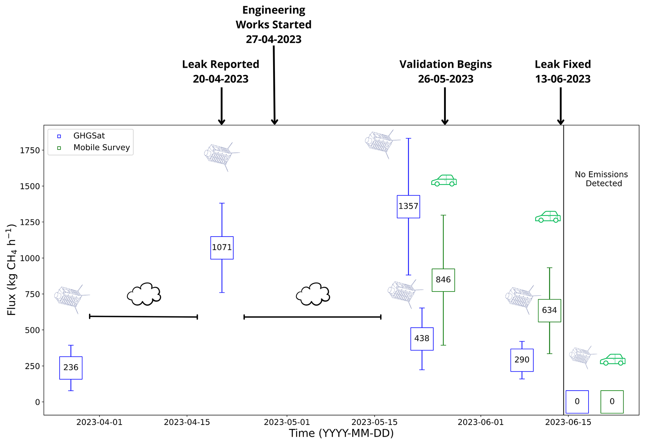
Figure 2 Timeline of events during the observation period of the gas leak and the flux estimates (kg CH₄ h⁻¹) from the different instruments. The satellite-derived fluxes are in blue, and the mobile-survey-derived fluxes are in green. The error bars represent the uncertainty on the flux estimates, as described in Sect. 2.3.1 and 2.3.2.

3.2 Flux estimations from NAME plume modelling

We also use NAME to obtain a modelled estimate of the gas leak on each observation date for GHGSat and mobile survey observations to allow continuity between different observation and flux estimation methods. We simulated the gas leak with a unit release (1 g s⁻¹) and then used the observed concentrations to scale NAME to estimate the flux as described in Sect. 2.4. Table 1 shows the flux estimations from GHGSat and the mobile survey and their corresponding NAME-derived flux estimation, with the bounds of the estimation quoted in brackets from NAME. The NAME-derived flux estimations are smaller than the GHGSat-derived fluxes but are always within the GHGSat uncertainty (Table 1). The smallest flux observed by GHGSat on 27 March was estimated to be 236 ± 157 kg h⁻¹, and we estimate a flux of 181 [135, 329] kg h⁻¹, with a difference of 23 % (55 kg h⁻¹) compared with the central estimate of the GHGSat-derived flux. The bounds of the NAME-derived flux estimations described in Sect. 2.4 are shown in brackets. The largest flux observed by GHGSat on 20 May was estimated to be 1375 ± 481 kg h⁻¹, and we estimate a flux of 1243 [931, 2322] kg h⁻¹, with a difference of 10 % (132 kg h⁻¹) compared with the central estimate of the GHGSat-derived flux. The estimation uncertainties for the NAME-derived fluxes are much larger than the GHGSat-derived fluxes on 20 April and 20 May, and this is likely due to the higher wind speeds used in the model compared with the wind speeds used in GHGSat's IME method (see Table S4).

Table 1 The comparison between the mobile-survey-derived and GHGSat-derived fluxes (kg h⁻¹) and the equivalent fluxes derived in NAME (kg h⁻¹). The bounds of NAME-derived fluxes are shown in brackets.

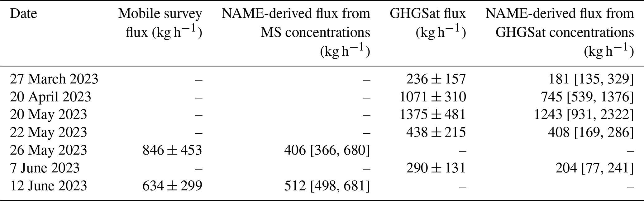
We also simulated the gas leak in NAME to derive a flux from the mobile survey observations. The NAME-derived fluxes are lower than the mobile-survey-derived fluxes, but they lie within the mobile survey estimation uncertainty (Table 1). The peak concentrations measured during the mobile survey were larger on 12 June than the concentrations measured on 26 May. However, the Gaussian plume model estimates a large flux on 26 May (846 ± 453 kg h⁻¹) due to differences in wind speeds on the observation days. The NAME-derived flux is larger on 12 June (512 [498, 681] kg h⁻¹) than the NAME-derived flux on 26 May (406 [366, 680] kg h⁻¹). The NAME-derived fluxes use the same wind speeds as the Gaussian plume model on 12 June, so differences between the model and the mobile survey fluxes are likely due to differences in the peak location along the road and the model resolution.

3.3 Modelled concentrations at tall tower site

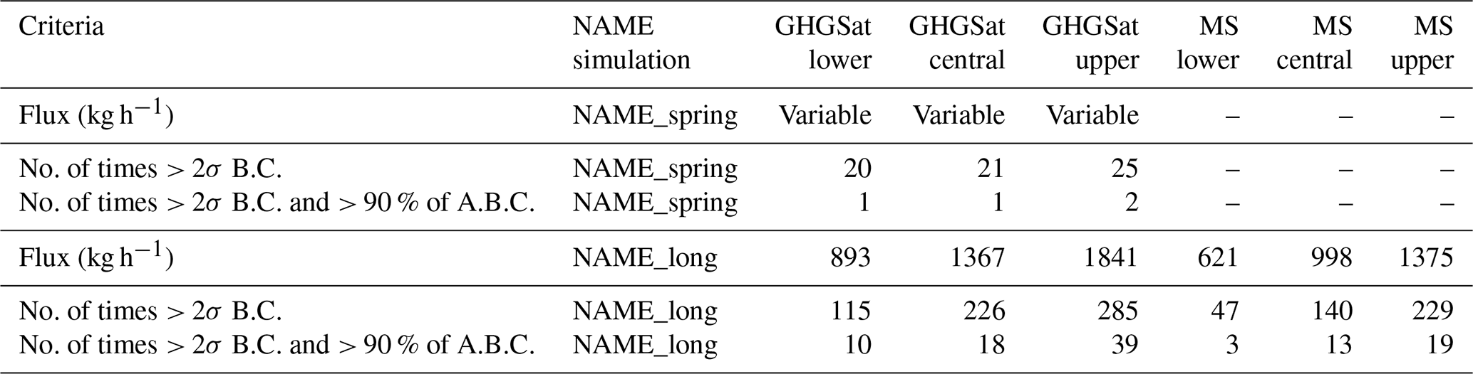
We carried out two simulations in NAME to assess the likelihood of the leak contributing to most of the observed above-background concentrations at RGL, described in Sect. 2.4. The occasions when the gas leak concentrations contribute to most of the above-background concentrations at RGL are defined as simulated concentrations that are at least 2 standard deviations (2σ, 14 ppb) larger than the observed background concentrations and contributing a significant percentage (≥ 90 %) of the above-background concentrations – we call this a “leak pollution event” (LPE). We investigated the number of LPEs at RGL over the period of the leak to assess whether statistical analysis and inverse modelling techniques might have been used to recognise the gas leak. Figure 3b shows that the observed above-background concentrations at RGL are almost always much larger than the contributions from the gas leak during the NAME_spring simulation. We calculated the number of times the gas leak concentrations at RGL met two different criteria. We first calculated the number of times the gas leak concentration was at least 2σ larger than the background concentration at RGL, i.e. when the leak's contribution was above the noise of the background concentrations. We also calculated the number of times the gas leak contributed to an LPE (> 2σ and > 90 % above-background) at RGL. Table 2 shows the results of these criteria during the NAME_spring simulation with hourly output. In the NAME_spring simulation, concentrations were above 2σ of the background concentrations 21 times and an LPE only occurred once. The enhancements due to the gas leak were larger than the noise of the background for at least 1 h on 8 of the 79 simulated days. The single pollution event from the NAME_spring simulation shows that although CH₄ from the gas leak can make up a large portion of the above-background concentrations at RGL, this does not happen frequently, and therefore it is not sufficient for statistical analysis or inverse modelling to identify the leak due to the significant contributions from other local sources.

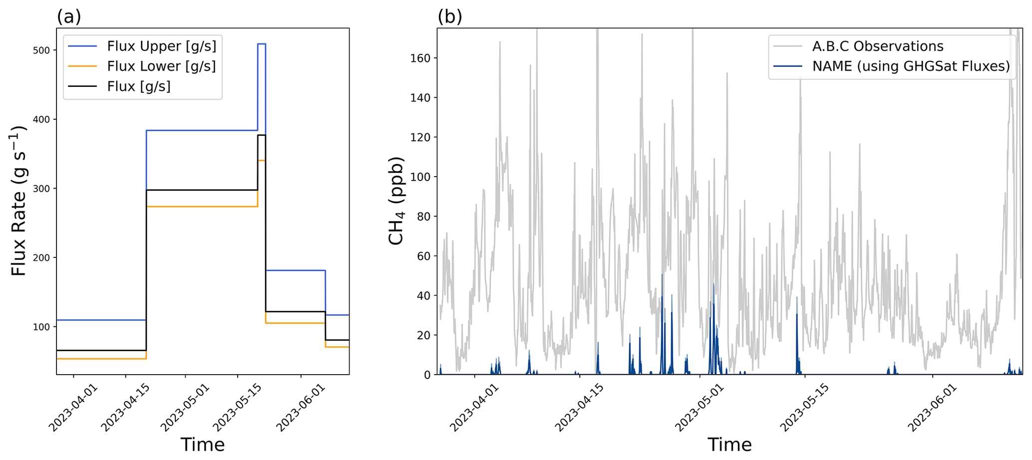
Figure 3 (a) Varying flux rates (g s⁻¹) used in the NAME model simulation “NAME-spring”. (b) Modelled CH₄ concentrations (ppb) at the Ridge Hill (RGL) tall tower site from GHGSat-derived flux rates in the NAME-spring simulation (blue) and observed above-background concentrations (A.B.C) at RGL (grey).

The results from the NAME_spring simulation show that the frequency of LPEs at RGL was low during the spring of 2023; therefore, we investigated the gas leak contribution at RGL over a longer period (“NAME_long”). The NAME_long simulation is a hypothetical situation in which the gas leak is emitting at its highest estimated rate (from both observation methods) for much longer than we actually observed the leak. Similar to the NAME_spring, the above-background concentrations at RGL during the NAME_long simulation period were much larger than the concentrations modelled from the gas leak at RGL, making it difficult to determine LPEs (see Fig. S8 in the Supplement). We applied the same criteria as the NAME_spring and found that during the NAME_long simulation the leak concentrations at RGL were 2σ above the background concentrations 226 times when using the GHGSat flux and 140 times when using the mobile survey flux. The gas leak was above the noise of the background concentrations for at least 1 h on 80 of 470 simulated days when using the satellite-derived flux. When we simulate the gas leak using the mobile-survey-derived flux we find the gas leak to be above the noise of background concentrations on 63 d for at least 1 h. The gas leak also meets the LPE criteria 18 times for the GHGSat flux and 13 times for the mobile survey flux. LPEs from the gas leak occurred on 12 of the 470 simulation days for at least 1 h when simulating the satellite-derived flux and on 7 d when simulating the mobile-survey-derived flux. The majority of the LPEs occurred during April 2023. Based on these figures, the frequency of LPEs from the gas leak during the NAME_long simulation is very low even when we assume that the gas leak is constantly emitted at the highest estimated flux rates. This means that it is difficult to recognise the gas leak above the noise of the background concentrations and to determine the flux of the gas leak using inverse modelling techniques and observations at RGL. Both the NAME_spring and NAME_long simulations show there is a low number of LPEs from the gas leak at RGL, which makes it difficult to recognise whether the above-background concentrations are from the leak or from other local sources.

Table 2 Number of 1 h periods of simulated concentrations at Ridge Hill from the gas leak were at least 2σ larger than the background concentrations (B.C.) and number of times a pollution event occurs (> 2σ B.C. and > 90 % of the above-background concentrations, A.B.C.). The columns denoted with “upper” and “lower” represent the upper- and lower-uncertainty flux from the satellite-derived and mobile-survey-derived (MS-derived) fluxes.

4 Discussion

In this study we detected, monitored and validated fluxes of a large gas leak from a low-pressure gas distribution pipe near Cheltenham, UK. The global monitoring satellite Sentinel-5P was not able to detect this leak during its overpass times because it was obstructed by clouds and the emission rate was lower than its theoretical detection threshold (25 000 kg h⁻¹; Lauvaux et al., 2022). The GHGSat detection threshold has a linear relationship with wind speed and is 100 kg h⁻¹ at 3 m s⁻¹ and 200 kg h⁻¹ at 6 m s⁻¹ (see McKeever and Jervis, 2022). GHGSat has demonstrated it can detect down to 42 kg h⁻¹ (McKeever and Jervis, 2022) and up to 79 000 kg h⁻¹ (GHGSat, 2022). As a result, the Cheltenham gas leak is well within the detection threshold of GHGSat. The high spectral resolution of GHGSat means that it is not affected by surface type as strongly as other satellites such as Sentinel-2 or Landsat. GHGSat has been tested across a mixture of surface types and found to have a column precision of ∼ 2 % (MacLean et al., 2024; Jacob et al., 2022). The GHGSat retrievals are predominantly during a northerly (N) or north-easterly (NE) wind, which means that the enhancement detected by the satellite was almost entirely from the leak due to few CH₄ sources upwind of the leak. The N/NE wind is useful for comparisons with the mobile survey and our tall tower model simulations because RGL is situated to the west of the gas leak. However, the first satellite retrieval on 27 March is during southerly wind. No emissions from the landfill were detected by GHGSat, which implies that emissions from the landfill are below 100 kg h⁻¹ and possibly lower than 42 kg h⁻¹. Also, by the time the landfill emissions reach the gas leak location, the CH₄ concentrations would be more diffuse, resulting in a very small percentage of the mole fraction in the retrieved pixel of the plume, so the effect of the landfill upwind of the gas leak on this day is considered negligible.

We also confirmed and assessed the leak by completing a mobile survey on 26 May and 22 June along the roads closest to the satellite-derived leak location. The mobile survey also sampled CH₄ concentrations on the roads closest to the nearby landfill sites but did not detect any CH₄ enhancements. The measured concentrations of the gas leak on 22 June were higher and the associated flux was lower than the equivalent concentrations and fluxes on 26 May, likely due to higher estimated wind speeds on 26 May. The Gaussian plume model has large uncertainties due to a number of factors, for example, the variability in the measured plume from changes in wind speed and direction, the lack of granularity in the Pasquill classification (Fredenslund et al., 2019) and the lack of certainty over the exact position of the leak itself.

The satellite-derived flux estimates and flux estimates based on the ground-based measurements display some differences. These could be due to actual differences in the leak rate on different days from changes in pipeline pressure or biases between the two measurement and flux estimation methods. There are significant uncertainties associated with both flux estimation methods which overlap for the satellite and mobile survey estimates on 22 and 26 May respectively. The second mobile survey resulted in similar fluxes to the first survey, and both were much larger than those estimated by GHGSat during the same week. Unfortunately, we were unable to obtain satellite retrievals on the same days as the mobile measurements due to obstruction by clouds. Since we were monitoring a live leak, it is likely that changes in flow through the pipe and engineering works will have caused variations in the flux, contributing to the differences between the satellite and mobile survey estimates. During the second mobile survey, on 12 June, repairs on the pipe were being carried out, so it is likely this estimate included more diffuse emissions from a wider area of excavated soil (see Fig. S1). More diffuse emissions could result in a wider CH₄ plume with lower concentrations which may not be above the threshold for enhanced CH₄ in the satellite retrievals. In addition to the effects of actual leak rate variations at the site, the satellite and mobile survey used different methods to estimate the fluxes, based on different meteorology. However, despite the mobile measurement fluxes being measured on different days, they agree well with the April and May satellite estimations. Based on the available observations, it is difficult to be certain whether the leak rate did drop in late May, as suggested by the GHGSat data, or continued at high rates, as suggested by the mobile survey.

The mobile survey allowed us to validate the gas leak by confirming the CH₄ detected by the satellite was present and through isotope measurements which also confirmed that the source was natural gas. While there are differences between the satellite-derived fluxes and the mobile-survey-derived fluxes, they are of the same magnitude, and differences could be due to the active nature of the leak.

The GHGSat Level 4 data, provided through the ESA TPM programme, give flux estimates for a source using GEOS FP wind data as standard. GHGSat would not normally have access to the higher-resolution UKV wind data. In order to provide some continuity between the different observation and flux estimation types, we calculated the flux of the gas leak using NAME based on the observed concentrations from the satellite retrievals and the mobile survey. We find that the NAME-derived fluxes follow the same temporal flux pattern but are slightly lower than the GHGSat flux estimations. The difference between the GHGSat-derived fluxes and the NAME-derived fluxes could be due to a number of reasons. The modelled and satellite-observed plumes did not overlap well, making it difficult to define a plume shape that fully captured the dispersion of the modelled plume. We employed a 25 m × 25 m horizontal resolution with 1.5 km resolution meteorology in NAME, which means the model might not capture local wind effects on the plume, leading to differences in the plume direction. The model simulations used a unit release, making it difficult to define the plume shape using the threshold value GHGSat applies to their retrievals (Jervis et al., 2021) or to apply any concentration thresholds based on the GHGSat retrievals because the modelled concentrations were not on the same scale. As a result, the criteria applied to the modelled plume, described in Sect. 2.4, are mostly independent from the satellite-derived plume apart from the length limit. The NAME-derived fluxes using the GHGSat concentrations are dependent on the plume selection criteria (see Table 1), particularly for larger fluxes, during 20 April and 20 May, where the bounds of the estimation are much larger. This could be due to different wind speeds used in the model and the IME method used by GHGSat when deriving the fluxes; the wind speed in NAME is generally higher than GEOS FP (see Table S4), and wind speeds are the largest uncertainty in the GHGSat IME flux estimation method (Jervis et al., 2021). On 22 May the main flux estimate is larger than the estimation bounds (408 [169, 286] kg h⁻¹), and this is due to the plume selection criteria on this day. When we remove values lower than 5 % of the maximum value, the modelled plume length remains larger than the observed plume, and as a result, the scaling factor is smaller, and the estimated flux is smaller than the main estimate. This is not the case for the other NAME-derived fluxes which use satellite observations. This further emphasises that the NAME-derived flux estimate is dependent on the plume selection criteria. We also applied a similar method to estimate the fluxes in NAME using the observations from the mobile survey. We find that the peak mixing ratios of the simulated plume do not align well with the peak mixing ratios from the mobile survey. This is likely due to the model meteorology not capturing local wind effects in this area. The road where the survey was conducted was approximately 30 m away from the estimated source location at its closest point, but at this location the car is either ascending or descending from the railway bridge, which is not fully accounted for in the model. We find that the NAME-derived fluxes using the mobile survey observations are smaller than the Gaussian plume model estimates, despite using the same wind speeds on 12 June. Differences between flux estimates could be due to different parametrisations in the NAME model compared with the Gaussian plume; for example, the Gaussian plume model assumes a neutral boundary layer and uses different dispersion assumptions. We are also sampling a very small section of the plume in the model, which might not fully represent the main peak of the plume but was chosen to be similar in distance between the estimated source location and mobile survey observations. Also, during the mobile survey, instantaneously measured concentrations from the gas leak fluctuated significantly whilst driving through the plume, showing predominately perturbations in atmospheric mixing. These effects are averaged out slightly when the emission is calculated because it incorporates multiple transects over a 30 min period, but some of these perturbations still remain, and the NAME model averages them out in the 1-hourly model time step.

The NAME-derived fluxes do provide some continuity between the different flux estimation methods because they show a similar temporal pattern. The NAME-derived fluxes still peak on 20 April and fluctuate in a similar pattern to the other estimation methods in May and June. This implies that there were fluctuations in the leaking gas, likely due to repairs on the pipe which were being carried out in May and June. The variation between the NAME-derived fluxes from both observation methods is smaller than the differences between the satellite-derived fluxes using the IME method and the mobile-survey-derived fluxes using the Gaussian plume method. This implies that the flux estimation methodologies are responsible for some differences between the satellite and mobile-survey-derived fluxes. In all three flux estimation methods the resolution of the wind data is much coarser than the size of the observed plume. Atmospheric transport at the surface through small-scale turbulence and influence of the local terrain may not be well represented, contributing to the uncertainty in the flux estimate. Also any systematic biases in the measurements or flux estimation methods are likely to be negligible in comparison to the uncertainties from wind speed and model uncertainties described in Sect. 2. Another uncertainty in modelling the flux in NAME from both the satellite and the mobile survey observations is the location of the leak. Four out of five locations were clustered together, and these were used to calculate the mean location for the NAME modelling and for the Gaussian plume modelling. One estimated location was positioned on the other side of the road to the actual leak and was considered an outlier. The mean location derived from the satellite data is approximately 30–40 m away from the engineering works (see Fig. S1). The location of the gas leaking into the atmosphere is not necessarily the location of the pipeline break. Wales & West Utilities (WWU) confirmed they replaced the whole pipe at once and so could not confirm the precise location of the leak. We cannot give an independent location due to lack of access to the area and no noticeable infrastructure to provide an estimate, resulting in the Gaussian plume model and NAME estimates being guided by the satellite-derived location. During the second ground-based mobile surveys we discovered an area of dead vegetation close to the satellite-derived location, which could be due to plants being suffocated by the amount of CH₄ (see Fig. S2); however, this is circumstantial.

To assess the impact of the source location on the NAME flux estimates we perturbed the leak location in the model by 10 m north (N), south (S), east (E) and west (W). We selected 10 m location perturbation to match the resolution of the NAME simulations using the surface-based observations. We kept the perturbations the same for the NAME simulations which use the satellite observations. Perturbing the source location shows that the mean location for the previous NAME simulations gives the lowest flux values. We also find that the flux estimations are lower than the satellite-derived fluxes, apart from on 20 May (see Table S3). The NAME fluxes, including the bounds of the estimation, derived on 20 May in the N, S, E, and W directions are all higher than the satellite-derived flux and the NAME-derived flux at the mean location. The wind speed remains the same as the original simulation for each perturbed location, and as a result, the maximum value of the plume was influenced most by the particles being advected by unresolved motions, such as turbulence, which are simulated by a random walk technique. This contributes to the uncertainty in the NAME-derived fluxes and shows that the flux estimation is dependent on the precise location of the leak when comparing with the IME and Gaussian-plume-model-derived fluxes. Large uncertainties occur when the fluxes are large (e.g. on 20 April and 20 May) or when estimated over a very small area (e.g. scaling the model using grid boxes along the road where the mobile survey measurements were taken).

In the NAME experiments, the maximum number of particles in the simulation can be adjusted so that the model does not stop producing particles during the simulation. We conducted all NAME runs with a maximum of 9×10⁷ particles. This value was selected in consultation with Met Office NAME scientists and was determined to be the optimal number for our high-resolution simulations. The final flux value is not sensitive to the number of particles because the total mass released (determined by the release rate) is distributed across the number of particles released.

Although the ground-based mobile-survey-derived fluxes and NAME-derived fluxes used independent observations and/or methodologies for the flux estimation, the assumed leak location was taken from the mean of GHGSat-derived location estimates. Despite using independent observations and models from the satellite data, it is noted that the flux estimates are not fully independent because we were unable to determine an independent estimate for the leak location.

We ran simulations in NAME to assess the frequency of the gas leak's contribution to the observed CH₄ at the nearby tall tower site, RGL. This method assumes that the meteorology and transport of CH₄ from the gas leak in the model are correct; however, it is likely that local meteorological effects and the surrounding terrain (e.g. the nearby railway bridge) will have had some influence the on transport of CH₄ from the gas leak to RGL. We assessed the frequency of pollution events during both our NAME_spring and NAME_long simulations and found a low number of LPEs. The results show that it is possible for the gas leak to contribute to an LPE at RGL. However, the low number of events means that it is difficult to estimate the location and magnitude of the flux using inverse modelling techniques. There are a number of different sources surrounding RGL which contribute to above-background concentrations such as agriculture, waste and fossil fuels from nearby towns and cities. When the wind is coming from the gas leak to RGL, the main sources near to the gas leak site are from pastoral and arable agriculture, household waste landfills, and food waste recycling. The addition of these other methane sources being transported to RGL also adds further complexity to the above-background signal at RGL.

The coverage of the tall tower network in the UK is sparse and not specifically designed for monitoring time-limited fugitive emissions like this gas leak, and these simulations show that it is unlikely that the RGL observations can be used to alert us to a gas leak of this size, location and duration. This highlights the importance of validating other observations methods, such as the GHGSat satellite constellation. In this case, it was fortuitous that the gas leak was close to a tall tower site at all; due to the sparse coverage of the UK DECC network, most gas leaks would likely not be near an observation site. Regular high-resolution satellite monitoring will allow us to detect emission locations, before monitoring them further through ground-based and drone-based surveys. GHGSat needs to be directed to observe the correct area in order to observe an emission, and it carries out daily “intelligence-led” targeting using information such as weather forecasts, past plume detection and locations of facilities likely to emit. However, a more robust “early-warning” system to alert GHGSat would be useful in determining locations for the satellite to target. For example, Schuit et al. (2023) have developed a machine learning model to detect emission plumes in Sentinel-5P measurements which allows GHGSat to identify and quantify emissions at a higher resolution. However, in this case the gas leak would not have been detected by Sentinel-5P, so other methods should be developed to detect smaller emissions. A disadvantage of monitoring methane emissions via satellite in the UK is that the country is often covered in clouds. However, GHGSat has a frequent revisit time of 1–2 d, and with more satellites coming online, there is an increased chance of a successful observation. A hybrid monitoring system combining satellite retrievals and mobile surveys could enable the operational detection of fugitive emissions and enhance countries' capabilities to reduce CH₄ emissions.

We investigated whether emission estimates from this gas leak would be reported in the UK's National Atmospheric Emissions Inventory (NAEI), which is funded by the UK Government's Department for Energy Security and Net Zero (DESNZ), and the Department for Environment, Food and Rural Affairs (DEFRA). The NAEI estimates emissions to the atmosphere from all anthropogenic sources, including CH₄, from gas leakage across the UK's National Transmission System (operated by National Grid) and the downstream gas networks that are operated by Wales & West Utilities (WWU) and other GDN operators (such as Cadent, Northern Gas Networks and SGN). The NAEI receives annual submissions from each of the GDNs to provide annual estimates of gas leakage from their distribution networks, using an industry-wide SLM. The SLM enables GDNs to apply consistent methods to generate emission estimates from several different source types across the gas network, with specific methods developed and agreed across the sector for above-ground installations (leakage and venting), low-pressure pipe leakage, medium-pressure pipe leakage, own gas use, and theft and third party damage. The annual gas leakage estimates are also reported by each of the GDNs to the Office of Gas and Electricity Markets (Ofgem; UK's independent energy regulator) as part of the network price control and performance mechanisms (Ofgem, 2023). For the gas leak detected by GHGSat, WWU would estimate the leakage of gas due as described in Marshall (2023), which would be included in the annual estimate reported to the NAEI. The annual submissions to the NAEI do not provide incident-specific estimates because the annual leakage estimates are aggregated prior to reporting to the NAEI. Therefore, the transparency and completeness of those reported emission estimates, including from third party damage incidents such as this gas leak, are uncertain.

In addition to detecting and monitoring the leak, GHGSat contacted the relevant utility company who took steps to fix the leak. The utility company confirmed that the leak was fixed on 13 June. This is a good example of how satellite data can be used to detect fugitive emissions and inform facility operators of their emissions, encouraging them to take action to fix leaks. We estimate that over 11 weeks with a mean emission rate of 754 kg h⁻¹, the pipeline would have leaked a total of 1 393 392 kg of CH₄. Using the United States Environmental Protection Agency's Greenhouse Gas Equivalencies Calculator (Greenhouse Gas Equivalencies Calculator, 2023), we estimate the mass of CH₄ lost to be 39 015 t of CO₂ equivalent, which is equivalent to the emissions from the average annual electricity consumption of 7500 homes.

5 Conclusion

In this study, we detected and monitored a gas leak from a low-pressure distribution pipeline near Cheltenham, UK, using GHGSat's high-resolution satellite constellation. We also validated the satellite-derived fluxes by completing two ground-based mobile greenhouse gas surveys and found differences with the satellite-derived fluxes, likely due to observations taking place on different days. During the observation period, the satellite-derived fluxes varied from 236–1357 kg h⁻¹, and the mobile-measurement-derived fluxes were between 634 and 846 kg h⁻¹. The mobile survey measurements agree better with earlier satellite estimates on 20 April and 20 May than the retrievals taken in late May and June covering the same weeks as the mobile survey, although they were not made concurrently with the satellite observations. We also estimated the gas leak flux using the NAME model to provide some continuity between the different flux estimation methods. We find that the fluxes in NAME are smaller than both the satellite- and mobile-survey-derived fluxes but are within the uncertainty of both and more consistent with each other. We also assessed the gas leak's contribution at the nearby tall tower site, RGL, although the UK DECC network is sparse and was not specifically designed to detect fugitive emissions. Our simulations show that for a gas leak 30 km from RGL we cannot provide a confident estimate of the flux rate using the RGL observations and inverse modelling techniques, and it was not likely that any significantly large above-background concentrations would have stood out in the observations.

Steps taken by GHGSat to inform the utility company also led to mitigation, which is a good example of how satellites can be used to aid companies and government bodies in reducing their emissions. This study shows that GHGSat has the capability to detect and monitor fugitive emissions over 100 kg h⁻¹ within the UK. The UK has access to mobile measurement laboratories, which can aid in monitoring CH₄ whilst the views from satellites are obscured by clouds. This gas leak was coincidentally discovered whilst trying to measure emissions from a nearby landfill. The discovery of this very large fugitive emission (by UK standards) raises the question of how many other large gas leaks are happening in the UK that are going undetected or unresolved. Although there are no current plans to carry this out operationally, combining satellite observations and mobile surveys means that the UK can access the technology to regularly monitor for fugitive emissions and take steps to significantly reduce their CH₄ emissions. It would seem prudent for the UK to explore how multiscale measurement methods currently used, primarily for academic research, can be moved into operational modes to assist with leak detection and repair programmes for the GDN. Currently, the focus on methane intensity and emissions reduction is on the upstream sector, but events such as these suggest that significant challenges face the distribution networks too.

This study highlights the capability of GHGSat and ground-based mobile surveys in monitoring fugitive emissions. Despite some differences in the emission estimates likely due to issues inherent in monitoring an active and variable leak, it is an excellent case study in validating satellite technology and collaborating with the industry to reduce the human impact on climate change.