Hybrid instrument network optimization for air quality monitoring

The significance of air quality monitoring for analyzing impact on public health is growing worldwide. A crucial part of smart city development includes deployment of suitable air pollution sensors at critical locations. Note that there are various air quality measurement instruments, ranging from expensive reference stations that provide accurate data to low-cost sensors that provide less accurate air quality measurements. In this research, we use a combination of sensors and monitors, which we call hybrid instruments, and focus on optimal placement of such instruments across a region. The objective of the problem is to maximize a satisfaction function that quantifies the weighted closeness of different regions to the places where such hybrid instruments are placed (here weights for different regions are quantified in terms of the relative population density and relative PM_2.5 concentration). Note that there can be several constraints such as those on budget, the minimum number of reference stations to be placed, or the set of important regions where at least one sensor should be placed. We develop two algorithms to solve this problem. The first one is a genetic algorithm that is a metaheuristic and that works on the principles of evolution. The second one is a greedy algorithm that selects the locally best choice in each iteration. We test these algorithms on different regions from India with varying sizes and other characteristics such as population distribution, PM_2.5 emissions, or available budget. The insights obtained from this paper can be used to quantitatively place reference stations and sensors in large cities rather than using ad hoc procedures or rules of thumb.

1 Introduction

According to the World Health Organization (WHO), ambient air pollution is a significant threat to people's health, causing around 6.7 million premature deaths annually in 2019 (Fuller et al., 2022). Shockingly, 99 % of the global population resides in areas that do not meet the WHO's air quality guidelines, with 89 % of these premature fatalities occurring in low- or middle-income countries (WHO, 2023; Pandey et al., 2021). To address this issue, it is crucial to develop suitable sensor networks by putting the air pollution monitors or sensors at appropriate locations, meeting the requirements of various groups in the city and providing much needed information. Air pollutant concentrations have traditionally been monitored using reference stations (we will refer to them as monitors in this paper), which are highly accurate but also very costly, limiting their widespread deployment (Lagerspetz et al., 2019). To achieve accurate air pollution monitoring within metropolitan regions, hundreds or even thousands of reference stations are required, which proves costly to maintain and operate (Zikova et al., 2017). However, the emergence of low-cost air quality sensors presents an opportunity for higher-density deployments and improved spatial resolution in monitoring (Spinelle et al., 2017; Castell et al., 2017). Low-cost sensors offer a cost-effective solution, reducing installation and maintenance expenses and facilitating broader spatial coverage, particularly in remote areas. Therefore, in order to balance the accuracy of monitoring along with costs involved in such instruments, we will consider deployment of both monitors and sensors in this paper.

Some studies focus on optimizing air quality monitoring networks (AQMNs) using different models: physical models (Araki et al., 2015; Hao and Xie, 2018) and learning-based models (Hsieh et al., 2015). However, the accuracy of these methods relies heavily on the precision of the air quality models, and both Hao and Xie (2018) and Hsieh et al. (2015) required existing air quality measurements as inputs for their prediction models, which largely depend on the quality and completeness of the input data. The studies by Li et al. (2017), Brienza et al. (2015), and Zikova et al. (2017) discuss ad hoc placement of air quality sensors in their respective study regions or use some rules of thumb. However, this shows that the placement of sensors is not optimized under the budget constraints that might be present. To address these challenges, it becomes crucial to develop more strategic approaches to place air quality sensors. Properly optimized sensor placement can lead to more comprehensive and accurate understanding of air pollution patterns, facilitating targeted pollution control measures and ultimately improving public health and environmental management.

Lerner et al. (2019) present a method for optimizing sensor placement based on sensor characteristics and land use analysis. Sun et al. (2019) also propose an optimal sensor placement strategy based on population density without relying on air pollution data. Their study highlights that humans naturally depend on the closest station to observe and obtain relevant information regarding the environment when multiple stations are present in a city. The satisfaction regarding the information increases as one moves closer to the adjacent station. Unlike Lerner et al. (2019), Sun et al. (2019) represent the benefit of placing a sensor in a particular grid to not only the citizens living in that grid but also to those living in the nearby grids. However, Sun et al. (2019) have limitations in that they do not incorporate air pollution data as a parameter in optimization, which raises concerns about the accuracy and reliability of the obtained results. Furthermore, both Lerner et al. (2019) and Sun et al. (2019) only consider deployment of one type of sensor, but as we discussed previously, both monitors (which are very accurate) and sensors (which are not that accurate but are much more economical than monitors) should be considered together for deployment.

Note that Castell et al. (2017) also highlighted that sensors alone may not provide accurate air quality measurements as compared to reference instruments or monitors. Our proposed approach aims to leverage the strengths of both sensors and monitors to enhance air quality monitoring in a cost-effective manner. We propose to develop a framework for placing hybrid instruments with the objective of maximizing public satisfaction by considering emission spread and population density as parameters (while considering the benefit of placing instruments in nearby grids and not just the grids where they are placed). Also, several notable constraints such as having at least one sensor in a given set of important grids (like important residential or commercial areas), not having monitors in certain given grids (like places with a sparse population or water bodies), or having a minimum number of grids where monitors should be placed in the network, have been proposed in the optimization formulation. Therefore, the following are the contributions of our work.

• Our research focuses on optimal deployment of hybrid air quality monitoring networks consisting of monitors and sensors where the goal is to maximize public satisfaction by providing accurate air quality information while considering several budget and other constraints.

• We propose a genetic algorithm (GA) and a greedy algorithm (GrA) to solve the developed optimization problem.

• We test the developed algorithms on networks of varying sizes and geographic locations.

This paper's remaining sections are organized as follows: Sect. 2 describes the optimization problem and presents the algorithms for solving the problem. The next section provides the numerical results tested using different algorithms under different settings. The final section concludes our study and provides future directions.

2 Methodology

This section is divided into two parts. The first part describes the problem statement for optimization of a hybrid instrument network. The second part describes the methods proposed to solve the optimization problem. The second part is further sub-divided into two sub-parts: genetic algorithm and greedy algorithm, respectively.

2.1 Problem statement

Our approach focuses on placing sensors and monitors in order to maximize a utility function quantifying popular satisfaction with the instrument placements. Realizing that humans naturally depend on the closest station to observe and obtain relevant information regarding the environment when multiple stations are present in a city, we assume that an individual's satisfaction g(d) is a function of his or her distance d to the closest sensor or monitor (Sun et al., 2019). Intuitively, the satisfaction with the information increases as one moves closer to the adjacent station. This is because people will have higher confidence in the readings by sensors or monitors that are closer to them rather than readings from instruments that are farther from them. Therefore, g(d) must satisfy the following conditions as stated in Sun et al. (2019): (i) g(d) must be a decreasing function; i.e., for any d₁≤d₂ we have g(d₁)≥g(d₂), and (ii) for any d≥0, g(d)≥0 and g(0)=1. The foremost condition corresponds to the relation of satisfaction function to distance, while the latter ones ensure the fact that the gϵ[0,1] and g is highest when the distance is zero. The following exponentially decreasing function g(d) readily satisfies the aforementioned conditions (Sun et al., 2019):

$$\begin{array}{}\text{(1)}& g\left(d\right)=\exp \left(-{\displaystyle \frac{d}{\mathit{\theta }}}\right),\end{array}$$

where θ is an exponential decay constant¹. The exponential decay function is often chosen in similar studies and practical applications because of its simplicity and effectiveness in modeling the attenuation of the signal or influence with increasing distance in studies such as Sun et al. (2019). It aligns with the intuitive idea that the influence of air quality monitoring decreases as one moves farther away from the monitor. We also present the results with another appropriate satisfaction function later. Note that monitors and sensors are not differentiated, while determining the satisfaction function in our problem. This is because, in many practical air quality monitoring scenarios, users may either not be interested or able to distinguish between the data collected from monitors and sensors (if the information related to the type of instrument is not openly available). From the user's perspective, the primary concern may be just to obtain reasonable air quality information rather than worry about the specific source of the data.

In accordance with the standard procedure for environmental monitoring (Krause et al., 2008; Hsieh et al., 2015), we divide the city into distinct, equally sized square grids. Then, we place our hybrid instruments (sensors and monitors) in these fragmented grids. Let $V=\left\{a\mathrm{|}a=\mathrm{1},\mathrm{2}\mathrm{\dots },n\right\}$ represent a set of grids in the interested geographical area, in which n=| V | represents the total number of grids. For each $a\in \left\{\mathrm{1},\mathrm{2},\mathrm{\dots },n\right\}$, let p_a represent the percentage of people living in grid a, e_a represent the percentage of PM_2.5 emissions² in grid a, and m_a denote the weighted average of p_a and e_a of grid a; i.e., $m_a=\left(w_{\mathrm{1}}\times p_a\right)+\left(w_{\mathrm{2}}\times e_a\right)$, where 0≤w₁, w₂≤1, and $w_{\mathrm{1}}+w_{\mathrm{2}}=\mathrm{1}$. Note that both population density and PM_2.5 emissions are important factors when deciding on the relative importance of various grids. Population density reflects the concentration of people residing in that grid, while the PM_2.5 emissions are an indicator of the level of fine particulate matter in the air within that grid (secondary aerosol production and pollution transport also play a role in the concentrations, but they are not considered here due to a lack of data). Finding a weighted average of the corresponding percentage values of these parameters provides a single value that quantifies the importance of a particular grid and allows comparison between different grids. Also, if we do not do the weighted averaging and individually minimize some metrics related to emission and population, this will result in a multi-objective optimization problem, which is much more difficult to solve and analyze (Deb, 2001).

We will now introduce some variables to define the optimization formulation. The notations are summarized in Appendix A. Let S be a set of grids where instruments (sensors and monitors) are placed (i.e., set S consists of each grid a such that at least a sensor or a monitor is placed at grid a). For each grid $a\in \left\{\mathrm{1},\mathrm{2},\mathrm{\dots },n\right\}$, let x_a be equal to 1 if a sensor is placed at grid a; otherwise, it is equal to 0. Let y_a be equal to 1 if a monitor is placed at grid a; otherwise, it is equal to 0. Let z_a be equal to 1 if any instrument is placed at grid a; otherwise, it is equal to 0. Let c be the cost of a sensor, c^′ be the cost of a monitor, and P be the total available budget. Let B be the set of grids where at least one sensor should be placed. Let C be the set of grids where a monitor cannot be placed. Let h be the minimum number of monitors that should be deployed. Let M be a very large positive number and m be a very small positive number. The formulation for optimally placing hybrid instruments is as follows.

$$\begin{array}{}\text{(2)}& {\displaystyle }max{\sum }_{a=\mathrm{1}}^n{m}_a\cdot g\left(d\left(a\right)\right)\text{(3)}& {\displaystyle }\text{s.t.}{\sum }_{a=\mathrm{1}}^n\left(c{x}_a+c^{\prime }{y}_a\right)\le P\text{(4)}& {\displaystyle }{\sum }_{a\mathit{ϵ}B}{x}_a\ge \mathrm{1}\text{(5)}& {\displaystyle }{\sum }_{a\mathit{ϵ}C}{y}_a=\mathrm{0}\text{(6)}& {\displaystyle }{\sum }_{a=\mathrm{1}}^n{y}_a\ge h\text{(7)}& {\displaystyle }M{z}_a+m\ge x_a+y_a,\forall a=\mathrm{1},\mathrm{2},\mathrm{\dots },n\text{(8)}& {\displaystyle }{x}_a+y_a\ge z_a,\forall a=\mathrm{1},\mathrm{2},\mathrm{\dots },n\end{array}$$

where $d\left(a\right)=\underset{b\in V}{min}\left\{z_b\cdot d(a,b)+\stackrel{\mathrm{‾}}{d}\left(a\right)\cdot \left(\mathrm{1}-z_b\right)\right\}$, and $\stackrel{\mathrm{‾}}{d}\left(a\right)=\underset{b\in V}{max}d(a,b)$.

The objective is to choose a subset of grids S⊆V that maximizes the overall satisfaction percentage under given constraints. Here, we define d(a, b) as the distance between grid a and grid b (note that, when we are finding distances between two grids, we mean distances between the centers of the grids), and d(a) is the minimal distance between grid a and any grid of set S (assuming that S is not an empty set, which is the case because of the constraint in Eq. 4). The condition in Eq. (3) is the budget constraint which states that the total cost of all the instruments cannot exceed P. The condition in Eq. (4) ensures that a sensor is placed in at least one of the grids belonging to set B. We do not impose analogous constraints such as Eq. (4) for monitors as monitors cannot be placed anywhere since they need electricity availability and they are big, heavy, and costly as compared to sensors. Equation (5) ensures that no monitor is placed at any grid belonging to set C (these grids can belong to locations like open areas or areas near water bodies). Note that it may not be cost-effective or practical to deploy expensive monitors in certain areas, and thus monitor deployments are restricted but sensor deployments are not. The condition in Eq. (6) ensures that at least h monitors are deployed. Equations (7) and (8) are the definitional constraints for variable z_a. That is, they ensure that, for each grid a, z_a is equal to 1 if $x_a+y_a\ge \mathrm{1}$. Otherwise, z_a is equal to 0.

As mentioned before, users may either not be interested or able to distinguish between the data collected from monitors and sensors. However, the network designer may be interested in distinguishing between the satisfaction obtained from the monitors and sensors. Therefore, we provide an alternate optimization formulation that distinguishes between the satisfaction obtained from monitors and sensors in Appendix B.

2.2 Methods

We will now present different algorithms to solve the proposed formulation. We will first introduce a genetic algorithm.

2.2.1 Genetic algorithm

A genetic algorithm is a metaheuristic that is inspired by the natural selection process and genetics (Deb, 2001). It mimics the principles of survival of the fittest, crossover, and mutation to iteratively search for optimal solutions. The algorithm starts by creating an initial population of potential solutions represented as strings of individuals. Consider a string comprising 2n elements (n is the total number of grids), where the first n elements are for the placement of the sensors and the next n elements are for the placement of the monitors. Each element in the string can take a value of either 0 or 1, where 1 indicates the presence of a sensor or monitor (depending on whether we are looking at the first n or last n elements) in the corresponding grid and 0 indicates their absence. We now consider a modification of the above string where we remove the elements that correspond to monitors belonging to set C. The removed elements will always have a value equal to 0 due to the definition of set C (consequently, monitors will not be placed on the grids belonging to the C set), and thus they are separated so that the values of these elements do not change due to the different processes in the GA. The aforementioned modified string is used in our problem. Each string encodes a set of decision variables representing a candidate solution to the problem.

We define a fitness metric that is used to assign a relative merit (fitness) to each solution based on the corresponding objective function value and constraint violations. The fitness, F(H), of any string H is calculated as follows:

$$\begin{array}{}\text{(9)}& \begin{array}{rl}& F\left(H\right)\\ & =\left\{\begin{array}{ll}\text{fn}& \text{if}H\text{is a feasible sol string},\\ {\mathrm{\text{fn}}}_{min}-D_{\mathrm{1}}-D_{\mathrm{2}}-D_{\mathrm{3}}& \text{otherwise},\end{array}\right.\end{array}\end{array}$$

where

$$\begin{array}{}\text{(10)}& {\displaystyle }\begin{array}{rl}& D_{\mathrm{1}}\\ & =\left\{\begin{array}{ll}\mathrm{0}& {\sum }_{a=\mathrm{1}}^n\left(c{x}_a+c^{\prime }{y}_a\right)\le P,\\ {\sum }_{a=\mathrm{1}}^n\left(c{x}_a+c^{{}^{\prime }}{y}_a\right)-P& \mathrm{\text{otherwise}},\end{array}\right.\end{array}\text{(11)}& {\displaystyle }{D}_{\mathrm{2}}=\left\{\begin{array}{ll}\mathrm{0}& {\sum }_{a\mathit{ϵ}B}{x}_a\ge \mathrm{1},\\ \mathrm{1}& \text{otherwise},\end{array}\right.\text{(12)}& {\displaystyle }{D}_{\mathrm{3}}=\left\{\begin{array}{ll}\mathrm{0}& {\sum }_{a=\mathrm{1}}^n{y}_a\ge h,\\ h-{\sum }_{a=\mathrm{1}}^n{y}_a& \text{otherwise}.\end{array}\right.\end{array}$$

Here, fn is the objective function value for string H as obtained by Eq. (2); fn_min is the minimum value of objective function values over all the feasible solution strings in a given population of strings; and D₁, D₂, and D₃ are penalty values for violating constraints in Eqs. (3), (4), and (6), respectively. Note that there is no penalty value for violating the constraint in Eq. (5), as that is automatically satisfied due to the way we define our strings (recall that we removed the elements corresponding to the grids of set C).

In each generation (or iteration) of the GA, roulette wheel selection (RWS) is used to select solutions from a population based on their fitness values (Deb, 2001). RWS provides a proportional selection mechanism where fitter solutions have a higher probability of being selected, but it still allows weaker solutions to have some chance of being chosen. After the selection procedure, a crossover procedure is followed where two strings are randomly selected from the mating pool, and a partial interchange from both strings is done to generate two new strings. We use the two-point crossover operator where two distinct crossover points divide the strings into three substrings and the middle substring is exchanged between the strings (Deb, 2001). After crossover, a mutation procedure is followed where the mutation operator alters from 1 to 0 or vice versa in each element of a string with probability P_m (referred to as the mutation probability). Note that mutation helps in maintaining diversity in the population. After applying the genetic operators, the parent population and offspring population are combined, strings in the combined population are sorted in non-increasing order, and the top half of the combined population is selected as the population for the next generation. This process is repeated over multiple iterations or generations until the termination criterion (to be specified next) is met. We now describe the termination criterion. Let the average fitness value of the strings in the population of the ith iteration or generation be k_i. Let N be the maximum number of iterations of the GA that are allowed. Then, the algorithm stops at the end of the ith iteration if $\left|\frac{k_i-k_{i-\mathrm{1}}}{k_{i-\mathrm{1}}}\right|\le \mathit{\alpha }$ (where α is a given value) or if i becomes equal to N.

2.2.2 Greedy algorithm

The second method to solve the optimization problem from Sect. 2.1 is a GrA. A greedy algorithm iteratively comes up with a solution by making choices that are locally optimal in each iteration, but it is not guaranteed to produce an optimal solution. In this algorithm, we first place a sensor at one of the locations from set B to satisfy Eq. (4). This placement is done by selecting the grid with the highest m_a among the set B. Then, we find the placement location for h monitors to satisfy Eq. (6) by ensuring that Eq. (5) (which tells us about the grids where monitors cannot be placed) is not violated. We now define the grid location s^∗ with the largest information gain as

$$s^{\ast }={\text{argmax}}_S{\sum }_{a=\mathrm{1}}^n{m}_a\left(g\left(d^{\prime }\left(a,K\cup s\right)\right)-g\left(d^{\prime }(a,K)\right)\right),$$

where K is the set of grids that have either a sensor or a monitor already placed (note that K is not an empty set because we have at least one grid belonging to set B that has a sensor placed) and $d^{\prime }(a,K)$ represents the minimum distance between grid a and any grid of set K. The placement of h monitors is done by repeatedly choosing the grid location with the largest information gain s^∗. Let $P^{\prime }=P$, where P^′ is the budget that remains after we subtract the cost of different instruments that are placed in different iterations of the GrA. After the placement of one sensor plus h monitors, the available budget is $P^{\prime }=P-c-h{c}^{\prime }$. After satisfying Eq. (6), there is no benefit to placing more monitors that are costly, and thus we target the placement of sensors. We keep placing sensors such that the grid location with the largest information gain s^∗ is selected while ensuring that P^′ is updated with every placement of sensor and budget constraint is satisfied. The algorithm terminates when there is an insufficient budget to place sensors, i.e., when $P^{\prime }<c$.

We now provide an example to illustrate the greedy algorithm in Appendix C.

3 Results

In this section, we will present results by testing our proposed algorithms in different settings. Our algorithms have been employed in two distinct areas within Surat and Mumbai. Both algorithms were implemented in MATLAB and executed on a computer with an Intel^® Core™ i7-2600 processor and 8 GB RAM (Ajnoti et al., 2024).

3.1 Surat

We first consider a portion of Surat, which is a major city in the state of Gujarat, India, for optimal placement of air quality instruments. In this study, we take a pilot project area of 5 km × 5 km in Surat and divide it into 25 grids (thus, each grid has a size of 1 km × 1 km). The total number of grids in Surat is 25; they are numbered from 1 to 25 from left to right in increasing order and from top to bottom in increasing order (see Table 1). To calculate the optimal locations for hybrid instruments, we use the average percentage of the population density (WorldPop provides open-source³ population density data at a spatial resolution of 1 km × 1 km) and PM_2.5 emissions data (The Energy and Resources Institute (TERI) provided us with PM_2.5 emissions data for Surat at a spatial resolution of 1 km × 1 km) for the part of Surat that we focus on. Figure 1 provides the intensity of population density (in population per square kilometer) and emissions (kT yr⁻¹) for the grids of Surat that are considered in this paper.

Table 1 Numbering of grids in the portion of Surat that is considered.

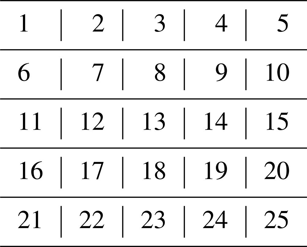
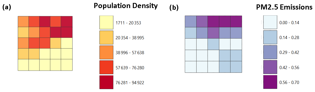
Figure 1 Intensities of population density for the considered grids of Surat (population per square kilometer) on the left and PM_2.5 emissions data for the considered grids of Surat (kT yr⁻¹) on the right.

Figure 2 displays the placement locations of sensors (purple points) and monitors (orange points) in Surat as obtained by a genetic algorithm (left) and a greedy algorithm (right) with a budget value of USD 295 000. Note that the objective function value corresponding to both the algorithms for this case is around 96.3 (see Fig. 3), but the spatial distribution of the instruments is not the same. This is because it is a discrete optimization problem and it is possible that two solutions with very different looking spatial distributions can have the same objective function value. Note that there is no scope to further add any instrument in the solution of any of the algorithms, as there are two monitors and 17 sensors and $\mathrm{2}\times \mathrm{122}\mathrm{000}+\mathrm{17}\times \mathrm{3000}=\mathrm{295}\mathrm{000}$. Also, note that the weights taken in the objective function are $w_{\mathrm{1}}=w_{\mathrm{2}}=\mathrm{0.5}$. This is because, by averaging these variables, we strike a balance between the need to monitor areas with high pollution levels (captured by PM_2.5 emissions) and areas with high population densities (captured by the population density). Note that we will present the sensitivity analysis with different weights later. The parameter values that are used in this placement are as follows: the cost of a sensor (c) is USD 3000, the cost of a monitor (c^′) is USD 122 000,⁴ the total available budget (P) is USD 295 000, and the values of θ and h are 1 and 2, respectively. The GA parameters that are used are as follows: the population size is equal to 1000, the mutation probability (P_m) is equal to 0.1, the maximum number of iterations or generations is 500, and the value of α is 10⁻⁵. Note that we determined that $\mathit{\alpha }={\mathrm{10}}^{-\mathrm{5}}$ consistently yielded satisfactory convergence while ensuring computational efficiency through systematic tuning involving a range of α values.

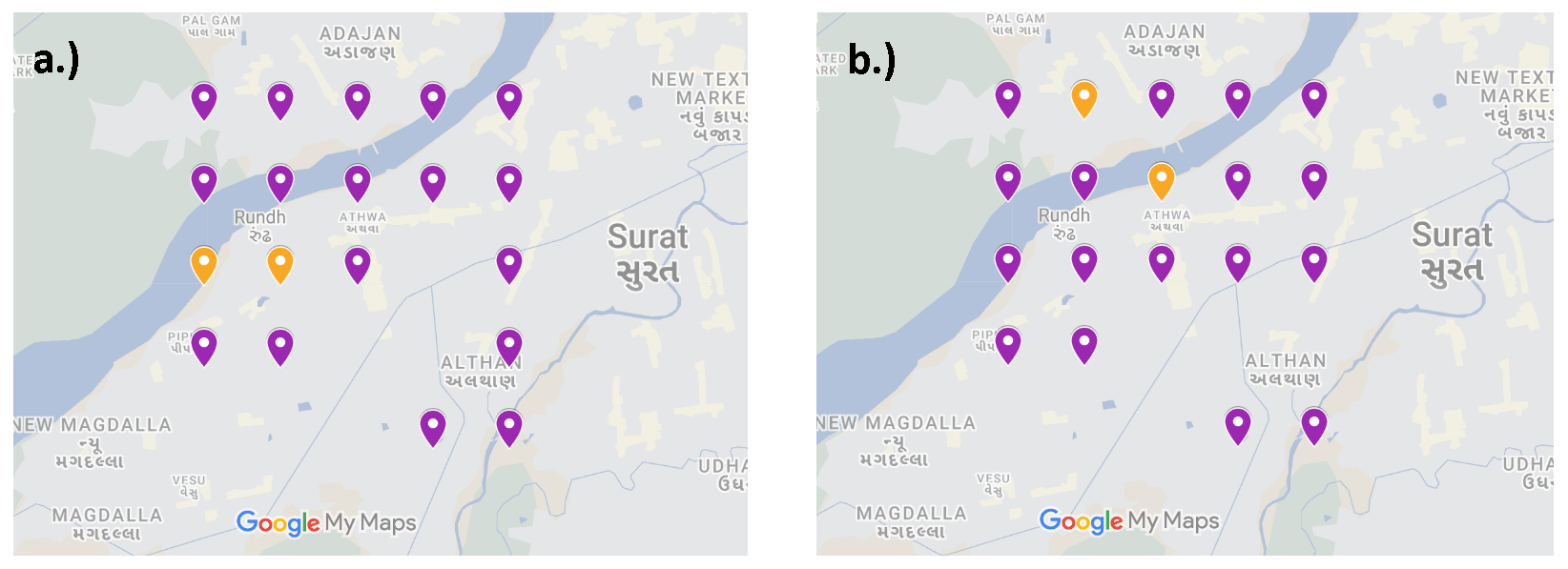
Figure 2 Hybrid placement obtained by the GA (a) and GrA (b) for the Surat network with a budget value of USD 295 000. Map data ©Google Maps 2023.

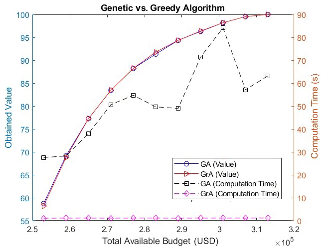
Figure 3 Plot comparing the genetic and greedy algorithms for varying total available budget values.

Figure 3 shows the values obtained and the computational time for the two algorithms, considering different total available budgets (i.e., P). Note that the obtained value on the vertical axis in Fig. 3 is an objective function value as given by Eq. (2). The minimum budget that is considered is USD 253 000, which is equal to the cost of three sensors plus h monitors (any value of the budget lower than this will not yield a feasible solution of the problem as the budget constraint will not be satisfied). The maximum budget in Fig. 3 is USD 313 000, which allows for the placement of two monitors and 23 sensors covering the entire portion area (as there are a total of 25 grids) under the minimum possible budget, as at least two monitors need to be placed by Eq. (6). Note that, if the budget is sufficiently large and the optimal solution involves covering all the grids, the GA can provide solutions where at some places interchanging sensors with monitors will not change the value of the solution. This is because the objective function does not differentiate between monitors and sensors and the solutions of the GA are generated through a probabilistic process and thus may exhibit a different spatial distribution than that obtained by the GrA.

From Fig. 3, it can be observed that, for most of the budget points, the obtained values for the GrA and GA are very close. Also, note that the obtained values for both the algorithms increase with the increase in the budget because it is possible to place more instruments with the increase in the budget, and this results in an increase in the overall satisfaction function value. Note that the computation time of the GA is significantly larger than that of the GrA because the GA samples through a set of possible solutions and iteratively applies various operators such as selection, crossover, and mutation, whereas the GrA is a deterministic algorithm that comes up with a single solution.

We provide an example in Appendix D to show the performance of different network configurations that have different variations with respect to the optimal solution.

3.1.1 Sensitivity analysis

In this section, we will present the results with a different g(d) function and consider different weights corresponding to p_a and e_a in the objective function.

Sensitivity analysis with another g(d) function

As previously mentioned, the g(d) function should be a decreasing function. Therefore, we explore an alternative function $g\left(d\right)=\frac{\mathrm{1}}{d+\mathrm{1}}$ apart from the exponential function. We have now obtained the results from a greedy algorithm and a genetic algorithm for the Surat network (5×5 size) using $g\left(d\right)=\frac{\mathrm{1}}{d+\mathrm{1}}$ while keeping all the other parameters the same (as in Fig. 3).

Figure 4 Plot comparing two functional forms of g(d).

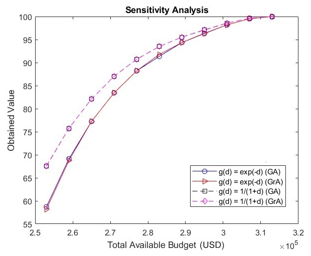
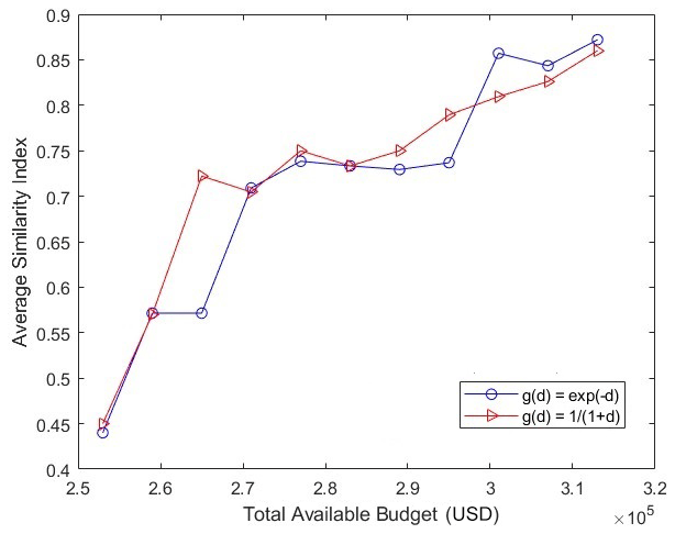
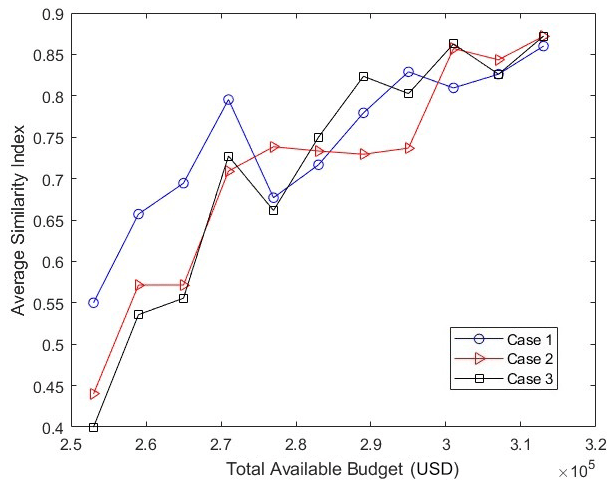
Figure 4 presents the values obtained by different algorithms and functional forms for g(d) with varying budget values. It can be seen in the above figure that the values obtained by the genetic algorithm and the greedy algorithm for $g\left(d\right)=e^{-d}$ are very close, and thus the solid-blue and red curves almost overlap. The same holds for $g\left(d\right)=\frac{\mathrm{1}}{d+\mathrm{1}}$, and therefore the dashed black and purple lines almost overlap. Note that the values that are obtained by the two algorithms for $g\left(d\right)=\frac{\mathrm{1}}{d+\mathrm{1}}$ are greater than those obtained for $g\left(d\right)=e^{-d}$. This is because $\frac{\mathrm{1}}{d+\mathrm{1}}>e^{-d}$ for all positive values of d. However, note that the pattern of the values that are obtained for the two functional forms is the same; i.e., the values decrease as the total available budget increases. Also, note that the values obtained by the two functional forms converge at the budget value of USD 313 000. Since it is not possible to have percentage values greater than 100, the values for both the functional forms will remain the same for budget values greater than USD 313 000. We believe that similar patterns will be observed by other functional forms of g(d) as long as they satisfy the conditions that are necessary for satisfaction functions (i.e., g(d) must be a decreasing function and g(0)=1). We have defined a similarity index that quantifies the difference in the placement of hybrid instruments as obtained by different algorithms. Suppose the number of grids where the placement of hybrid instruments by the two algorithms is identical is given by k (a grid is said to have identical placement by the two algorithms if the grid contains a sensor as determined by both the algorithms or a monitor as determined by both the algorithms). Also, let the maximum number of hybrid instruments that can be placed in the given constraints be equal to p. Then, the similarity index is given by $k/p$. Since the solution obtained by the genetic algorithm is probabilistic, we tested five runs of the genetic algorithm (for a given budget value) and compared the solution obtained by each run to the solution obtained by the greedy algorithm to determine the similarity indices and finally obtained the average similarity index by taking the mean of the five similarity indices. Figure 5 shows the average similarity index for different budget values and for different g(d) functions (while keeping equal weights for the percentages of the population density and emissions). Note that the similarity index is upper-bounded by 1. Also, we see that, as budget values increase, the average similarity index for both g(d) functions increases. This is because, as the budget increases, the number of grids at which instruments can be placed increases and both the algorithms usually place sensors at most of the grids, except at a few grids where monitors are placed to meet the requirement of the minimum monitors. Note that the average similarity index is around 0.5 for low budget values due to the existence of solutions that have varying placements but have close objective function values (but as the budget increases, the variation in the placement decreases, as explained before). Also, the average similarity indices obtained by the two g(d) functions are close for most of the budget values.

Figure 5 Average similarity index for different g(d) functions.

Sensitivity analysis for different weights in the objective function

We have also conducted the sensitivity analysis by varying the weights between the percentages of population density and PM_2.5 emissions (i.e., p_a and e_a) for Surat. Table 2 shows the weights corresponding to the different cases that have been considered. We have determined the results for both the greedy algorithm and the genetic algorithm by keeping all the parameters the same (as in Fig. 3).

Table 2 Different cases for the weights.

Figure 6 Plot comparing cases for different weights corresponding to p_a and e_a.

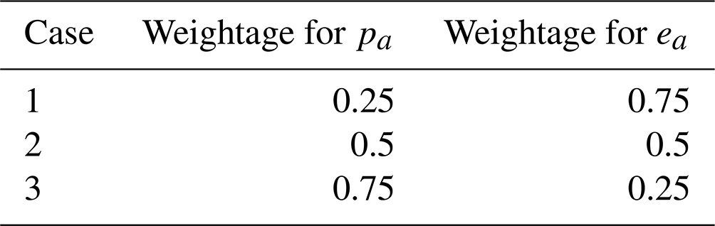
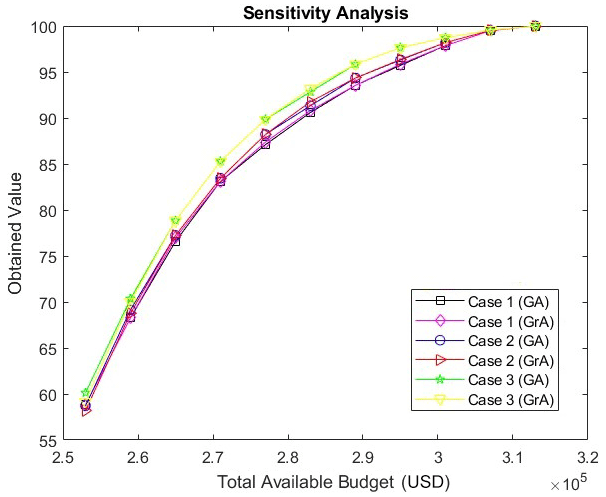
Figure 6 shows the values that are obtained for different cases, budget values, and algorithms. As before, the values obtained by the GA and GrA are very close for the given weights and budget. Among these cases, the values corresponding to Case 3 (where p_a=0.75 and e_a=0.25) are the highest and those corresponding to Case 1 (where p_a=0.25 and e_a=0.75) are the lowest. Thus, as the relative weightage for population density increases in the objective function, the values obtained increase. However, it can be seen that the difference between the values for Cases 1 and 3 is not that large, signifying that the objective function values may not be that sensitive to the relative weightage between population density and emissions. Figure 7 shows the average similarity index for different budget values and different cases corresponding to the weights of the percentages of population density and PM_2.5 emissions (while keeping g(d) as the exponential function). It can be seen that the average similarity index increases with budget values for the same reason as mentioned for Fig. 5. Also, the values of the similarity indices are close for most of the budget values.

Figure 7 Average similarity index for different weights corresponding to p_a and e_a.

3.2 Mumbai

We now present the results that we tested for portions of Mumbai, which is the financial hub of India. In this case, we only considered the contribution of population in the objective function (i.e., w₁=1, w₂=0, implying m_a=p_a) due to unavailability of PM_2.5 emissions data for Mumbai. However, the aforementioned change does not have any significant relevance to the results that we present as we plan to test the effect of varying the budget (as in the last section) and the effect of varying the size of the network (i.e., the number of grids). All the parameter values for the algorithm's execution were the same as in the example for Surat (i.e., Fig. 3), except for the variable θ, which has now been set to 5 (note that θ has been increased now because we have a larger number of grids in the Mumbai network as compared to Surat, resulting in higher average distances between the grids for the Mumbai network, and thus we need to update θ for better normalization). Consider a region of size 10 km × 10 km in Mumbai that has been divided into 100 grids (i.e., each grid has a size of 1 km × 1 km). Figure 8 shows the variation of the values obtained and the computation time with the total available budget for the GA and GrA for this region. The solid lines represent the obtained values, and the dashed lines are used to represent the computation time in seconds for different algorithms. It can be seen that the GA provides a higher value as compared to the GrA for most of the cases. Thus, this highlights the importance of the GA in obtaining values that are closer to the optimal ones as compared to the GrA when the network size increased (however, this advantage comes at the high computational cost of the GA as compared to the GrA).

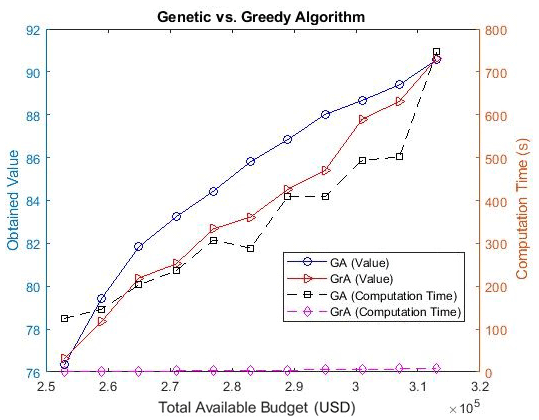
Figure 8 Plot comparing the genetic and greedy algorithms for varying total available budget values.

Figure 9 shows the placement of hybrid instruments obtained for the two algorithms (GA and GrA) when the budget is equal to USD 283 000 when we have all the other parameters the same as those in Fig. 8. The blue and orange points represent the placements of the sensors and monitors, respectively. In Fig. 9a, two sensors are positioned in the northeastern area, while no sensors or monitors are placed in that area in Fig. 9b. In Fig. 9b, monitors and sensors are predominantly concentrated on the left side of the Mumbai area, whereas in Fig. 9a, the sensors and monitors exhibit a more diverse and scattered distribution. Note that, out of 100 grids, sensors and monitors can be placed in only 15 grids by maximizing the objective function. The leftmost and southern areas have the highest population density, which explains the concentration of the sensors and monitors in those regions. There is a difference in the solutions that are obtained by the two algorithms because the GA samples through various solutions to proceed towards a solution is closer to the optimal one, whereas the GrA is a deterministic algorithm and may get stuck near a locally optimal solution.

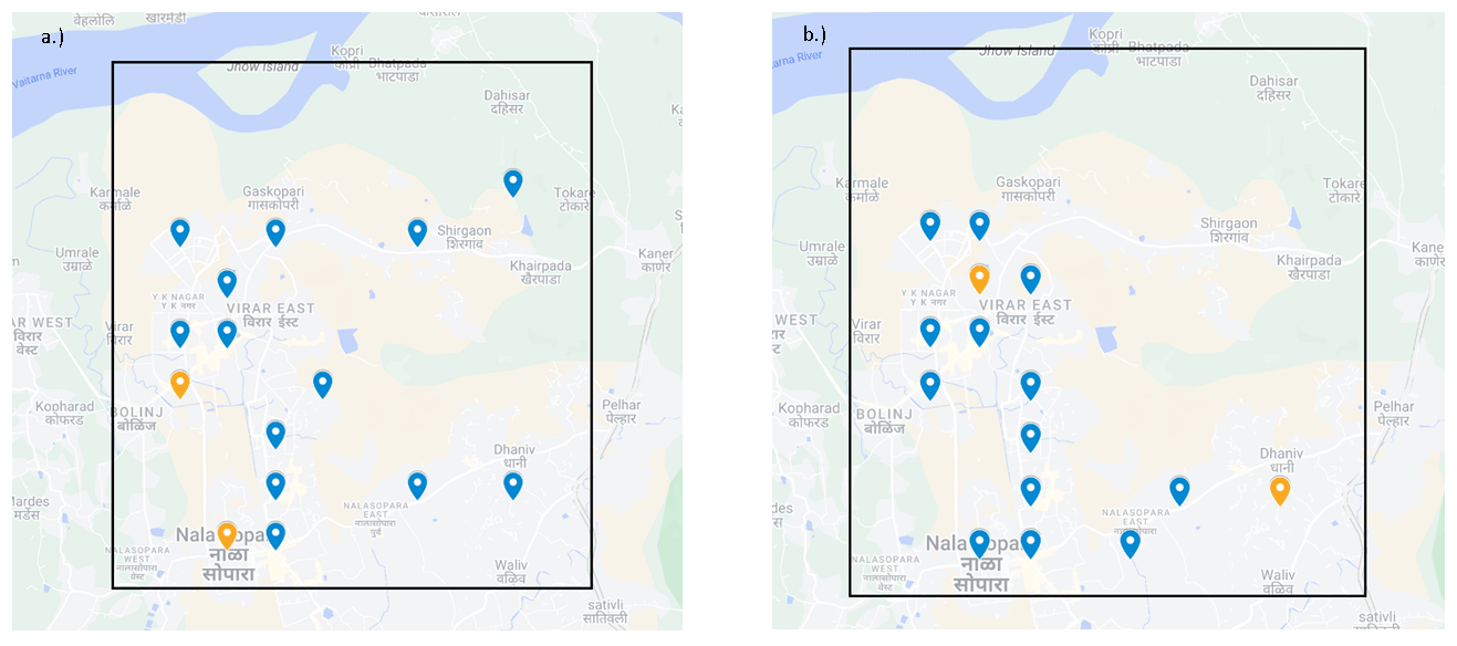
Figure 9 Sensor placement obtained by the GA (a) and GrA (b) for the 10 km × 10 km (100-grid) region in Mumbai when the budget is equal to USD 283 000. Map data © Google Maps 2023.

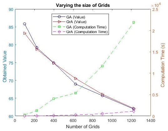
Figure 10 shows the comparison between the GA and GrA with varying numbers of grids for the budget value of USD 283 000.⁵ The solid lines represent the obtained values in the percentage for the different algorithms, and the dashed lines are used to represent the computation time in seconds for the different algorithms. As the number of grids increases, there is a noticeable decline in citizen satisfaction (i.e., the obtained values) because the budget P remains the same and thus the satisfaction averaged across all the grids reduces as it is distributed across the total region (note that the percentage of the population in each grid also decreases as the number of grids increases and thus also contributes to the observed trend). Also, the values obtained by the GA and GrA are similar, and in some cases the GA outperforms the GrA, whereas the reverse happens in the other cases. Note that the computation time required for the GA increases rapidly with the increase in the number of grids, because with the increase in the number of grids, the size of each string in the GA increases and it takes more iterations before the termination criterion is reached in the GA (as the number of feasible solutions increases with the increase in grid size). However, the increase in the computational time of the GrA is not that high, as it is a polynomial–time algorithm (Cormen et al., 2022); i.e., the computational time increases polynomially with respect to the increase in the problem size (i.e., the number of grids in our problem).

Figure 10 Plot comparing the genetic and greedy algorithms for a varying number of grids.

4 Conclusions

This research paper proposed an optimization formulation for placement of hybrid instruments (sensors and monitors). The objective of the problem is to maximize the satisfaction function while satisfying various constraints for the placement. To solve this formulation, we proposed two algorithms: a genetic algorithm (GA), which is a metaheuristic that works using the principles of evolution, and a greedy algorithm (GrA), which makes choices that are locally optimal in each iteration. We tested the placement solutions generated by these algorithms on networks from different locations (Surat and Mumbai) that differed over sizes and characteristics (population distribution, budget, and PM_2.5 distribution). We observed that, as the total available budget increased, the obtained values from the two algorithms also increased as it became possible to place more instruments (sensors and monitors). We found that the GrA is very computationally efficient as compared to the GA, but we found that both the GrA and GA provided close values (in some cases the GA outperformed the GrA, whereas in other cases the reverse happened). Note that since the GA searches through a set of solutions over multiple iterations and uses operators like mutation, it has a better likelihood of getting towards the optimal solutions, whereas the GrA may get stuck near a local optimum in some cases. These findings suggest that, if time is not constrained (i.e., we have a few days to decide on the placement solution), it might be better to use the GA and GrA together (i.e., use the best solution out of the two algorithms) to place the instruments, whereas in scenarios where there is a scarcity of time, it is advisable to use the GrA. While the study's results are specific to these locations, the underlying methodology and principles learned from these cases can be broadly applied to other areas facing similar air quality monitoring challenges. The methodology presented in our paper serves as a template for optimizing sensor networks in any location, provided that relevant data on population, emissions, and potential grid locations are available. Our research aims to provide valuable insights for future government decision-making processes regarding the optimal deployment of hybrid instruments in cities lacking an existing sensor network.

There are several interesting future extensions of this work that are possible. We acknowledge the challenges associated with quantifying PM_2.5 emissions in areas lacking an established monitoring network, as evident in the Mumbai case. However, in future, solutions such as considering existing models or satellite-derived data as proxies for local PM_2.5 concentrations during the network design phase can be implemented. Also, after the placement of the instruments, one could iteratively update the placement of the network using some existing models or proxy data, as newly collected data update the prior estimates of concentrations in the different grid cells. In addition, we assumed a particular form of the satisfaction function (consisting of exponential terms), but other forms can also be tested. Similarly, other factors apart from population density and PM_2.5 concentrations such as socioeconomic disparities across various grids can also be factored while determining the satisfaction function. Note that exploring other objective functions, such as improving estimates of population exposure or monitoring the largest known sources, would also be very interesting. To address these alternative objectives, we could make the following modifications to our approach. First, the objective function could be defined appropriately, whether it is optimizing public satisfaction, estimating exposure, or addressing specific environmental issues. Also, depending on the chosen objective, we may need to adapt the data collection methods used. For example, if the goal is to estimate population exposure, we may need to tailor the data collection frequency accordingly. The analysis methods and models used for decision-making can be customized based on the objective. For instance, if the goal is to address specific environmental concerns, sophisticated modeling techniques may be employed to assess pollutant dispersion. When other objective functions are used, the fitness function in the genetic algorithm will be modified. The selection, crossover, and mutation operators will not change if the constraints remain the same, and there would only be a change in the objective function. Similarly, the greedy algorithm will have a modified gain function s^∗ and the rest of the algorithm will remain the same provided the constraints in the problem remain the same. Thus, our approach can be flexibly adapted to address a range of objectives. Note that there is also potential for creating user-friendly software tools or decision support systems based on the methodology presented in our paper. Such tools would enable users with limited algorithmic expertise to apply similar optimization techniques to their specific locations, addressing the concern of not having the ability to run the algorithm. In these software tools, the users will only have to provide input values for the problem, e.g., the network they want to solve, the costs of the instruments, the budget, or the algorithm they want to use, and the toolbox will provide the results.

Appendix A

Notations	Description
V	Set of all grids
n	Total number of grids
S	Set of grids selected for deploying hybrid instruments
g(d)	An individual's satisfaction as a function of his or her distance d to the closest sensor or monitor
θ	Exponential decay parameter
pa	Percentage of the population living in grid a
ea	Percentage of the concentration of PM2.5 in grid a
ma	Weighted average of pa and ea
c	Cost of each sensor
c′	Cost of each monitor
P	Total available budget
h	Minimum number of monitors to be deployed
za	Binary variable signifying whether a sensor or a monitor is placed at grid a or not
xa	Binary variable signifying whether a sensor is placed at grid a or not
ya	Binary variable signifying whether a monitor is placed at grid a or not
B	Set of grids where at least one sensor is to be placed
C	Set of grids where monitors cannot be placed
M	A very large positive number
m	A very small positive number
Pm	Mutation probability
N	Maximum number of iterations of the GA that are allowed
d(a)	Minimum distance between grid a and the grids containing hybrid instruments
d(a,b)	Distance between grid a and grid b
$\stackrel{\mathrm{‾}}{d}\left(a\right)$	Maximum distance between grid a and any other grid of set V
$d^{\prime }\left(a,K\right)$	Minimum distance between grid a and set K

Appendix B

We provide an alternative optimization formulation whose objective is to maximize the weighted sum of satisfaction functions from monitors and sensors. Let w_s be the weight corresponding to the satisfaction from sensors and w_m be the weight corresponding to the satisfaction from monitors. Let d(a) be the minimum distance between grid a and any grid containing sensors, and let d^′(a) be the minimum distance between grid a and any grid containing monitors. The remaining parameters and variables mean the same as before. Then, the formulation is as follows:

$$\begin{array}{}\text{(B1)}& {\displaystyle }max{w}_{\mathrm{s}}{\sum }_{a=\mathrm{1}}^n{m}_a\cdot g\left(d\left(a\right)\right)+w_{\mathrm{m}}{\sum }_{a=\mathrm{1}}^n{m}_a\cdot g\left(d^{\prime }\left(a\right)\right),\text{(B2)}& {\displaystyle }\text{s.t.}\sum _{a=\mathrm{1}}^n\left(c{x}_a+c^{\prime }{y}_a\right)\le P,\text{(B3)}& {\displaystyle }{\sum }_{a\mathit{ϵ}B}{x}_a\ge \mathrm{1},\text{(B4)}& {\displaystyle }{\sum }_{a\mathit{ϵ}C}{y}_a=\mathrm{0},\text{(B5)}& {\displaystyle }{\sum }_{a=\mathrm{1}}^n{y}_a\ge h,\end{array}$$

where

$$\begin{array}{c}{\displaystyle }d\left(a\right)=\underset{b\in V}{min}\left\{x_b\cdot d(a,b)+\stackrel{\mathrm{‾}}{d}\left(a\right)\cdot \left(\mathrm{1}-x_b\right)\right\},\\ {\displaystyle }\stackrel{\mathrm{‾}}{d}\left(a\right)=\underset{b\in V}{max}d(a,b),\text{and}\\ {\displaystyle }{d}^{\prime }\left(a\right)=\underset{b\in V}{min}\left\{y_b\cdot d(a,b)+\stackrel{\mathrm{‾}}{d}\left(a\right)\cdot \left(\mathrm{1}-y_b\right)\right\}.\end{array}$$

Thus, the relative values of the weights w_s and w_m decide the relative importance being given to sensors and monitors. Typically, w_m should be chosen larger than w_s as monitors are more accurate than sensors. One could solve the above formulation with minimal changes to the proposed genetic and greedy algorithms.

Appendix C

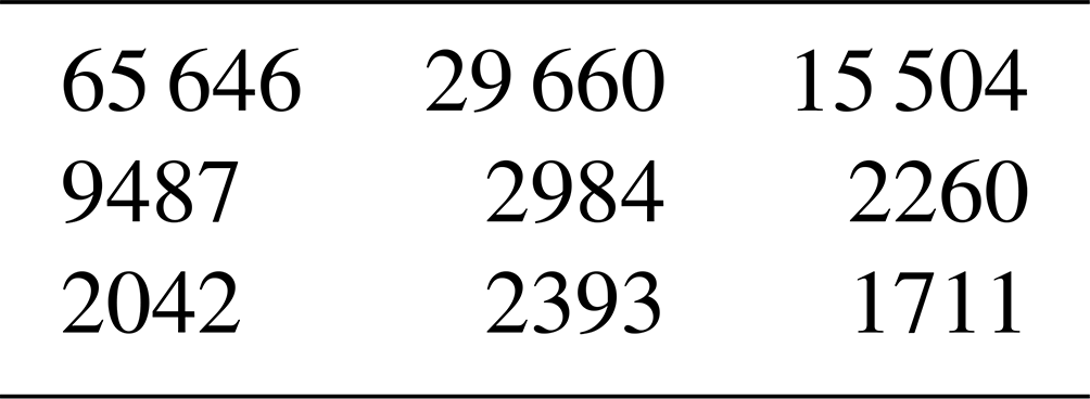
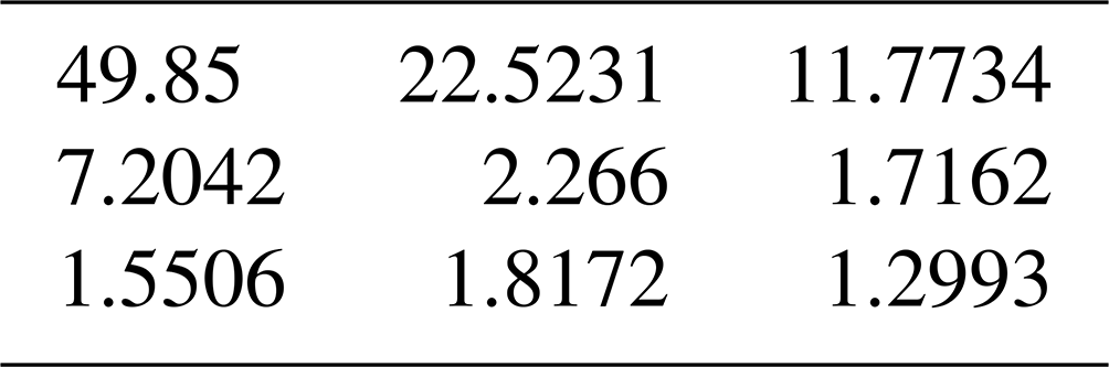
We now provide an example of a 3×3 network (i.e., a network with $\mathrm{3}\times \mathrm{3}=\mathrm{9}$ grids) to illustrate the greedy algorithm. The population density data (in population per square kilometer) and PM_2.5 emissions data (kT yr⁻¹) for a 3×3 network are provided in Tables C1 and C2, respectively.

Table C1 Population density data.

Table C2 PM_2.5 emissions data.

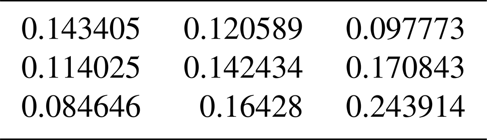
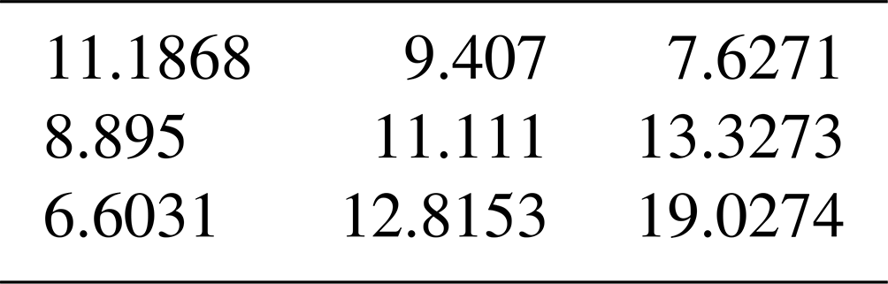
Then, we calculate the percentage of population density (p_a) and PM_2.5 emissions (e_a) for each grid and then calculate m_a, which is an average of p_a and e_a. Tables C3 and C4 show the values of p_a and e_a, respectively.

Table C3 Percentage of population density.

Table C4 Percentage of PM_2.5 emissions.

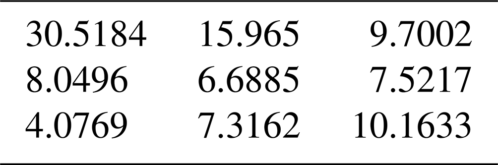
The following values are the m_a values for each grid of the 3×3 network that we consider.

Table C5 Average of the percentages of population density and PM_2.5 emissions.

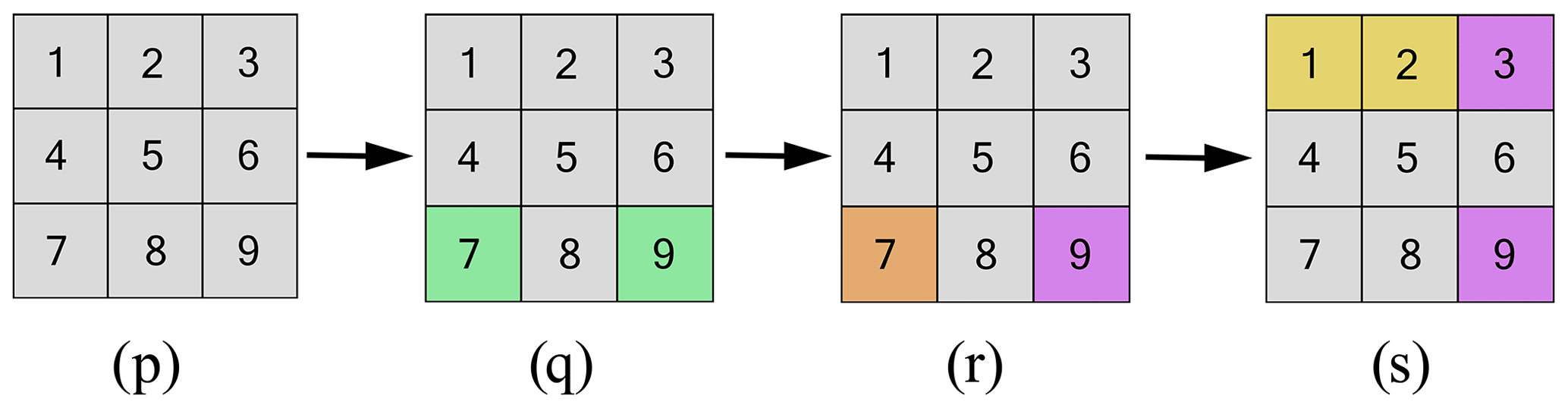
Suppose the set B in which at least one sensor is to be placed from Eq. (4) consists of grids 7 and 9, and set C in which no monitor can be placed from Eq. (5) is given by set 7. Suppose h=2, which represents the minimum number of monitors required. Let the cost of the sensor (c) and monitor (c^′) be 200 and 8000 units, respectively. The total available budget is 16 500 units.

Figure C1p shows the initial empty grids, which are grey in color. Figure C1q shows the grid area in which two grids (i.e., grids 7 and 9) are shown in light-green-colored grids, which tells us about grids in set B, where at least one sensor must be placed. Given that the value of m_a for grid 9 is greater than that of grid 7, a sensor is initially placed at grid 9 to satisfy Eq. (4). The placement of a sensor at grid 9 reduces the available budget to 16 300 units.

Figure C1r shows the placement of a sensor at grid 9 and a grid (corresponding to set C) which is shown by an orange-colored square grid (i.e., grid 7). The monitors are positioned at grids 1 and 2 based on the values obtained from the largest information gain s^∗ and in adherence to Eq. (5), which has a requirement that no monitor be placed on any grid belonging to set C. This further reduces the budget from 16 300 to 300 units by subtracting 16 000 units (i.e., c^′h).

We continue to place sensors until the budget constraint is violated. We will place the next sensor at the grid with the largest information gain s^∗, and that grid is grid 3. This further reduces the budget from 300 to 100 units. The algorithm stops here as there is no sufficient budget to proceed. Figure C1s shows the final solution using the greedy algorithm, where grey-colored square grids show the empty grids, purple-colored square grids show the placement locations of the sensors, and light-yellow-colored square grids show the placement locations of the monitors.

Figure C1 Example to show the working of the greedy algorithm.

Appendix D

We present an example to show the performance of different network configurations that have different variations with respect to the optimal solution. Consider an example of a 3×3 network. Let the cost of a sensor (c) and a monitor (c^′) be USD 3000 and 122 000, respectively. Suppose the budget value is equal to USD 253 000. The numbering of the grids follows the convention that numbers first increase as we go from left to right in increasing order and numbers increase as we go from top to bottom. Let set B in which at least one sensor is to be placed from Eq. (4) consist of grids 7 and 9, and let set C in which no monitor can be placed from Eq. (5) be set 7. We consider four different feasible solutions as follows.

Case 1. The solution is obtained from the greedy algorithm.

Figure D1 shows the solution that is obtained in Case 1. The purple points show the placement locations of sensors, and orange points show the placement locations of monitors. It can be seen that monitors are placed at grids 1 and 2 and that sensors are placed at grids 3, 4, and 9.

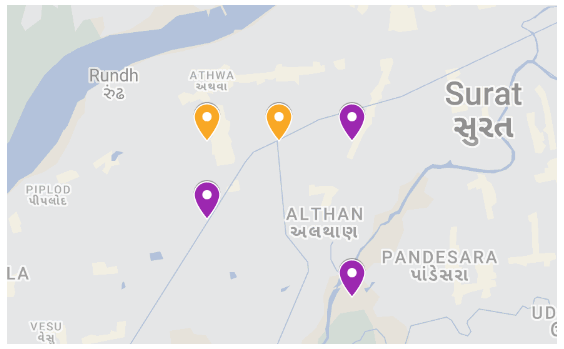
Figure D1 Hybrid placement obtained from the GrA. Map data © Google Maps 2023.

Case 2. The sensor placed at grid 3 in Case 1 is moved to grid 7 (all the other instrument locations remain the same as in Case 1).

Case 3. The monitor placed at grid 1 in Case 1 is moved to grid 5 (all the other instrument locations remain the same as in Case 1).

Case 4. The sensor placed at grid 3 in Case 1 is moved to grid 7, and the monitor placed at grid 1 in Case 1 is moved to grid 5 (all the other instrument locations remain the same as in Case 1).

Table D1 shows the values that are obtained for the different cases.

Table D1 Values obtained for different cases.

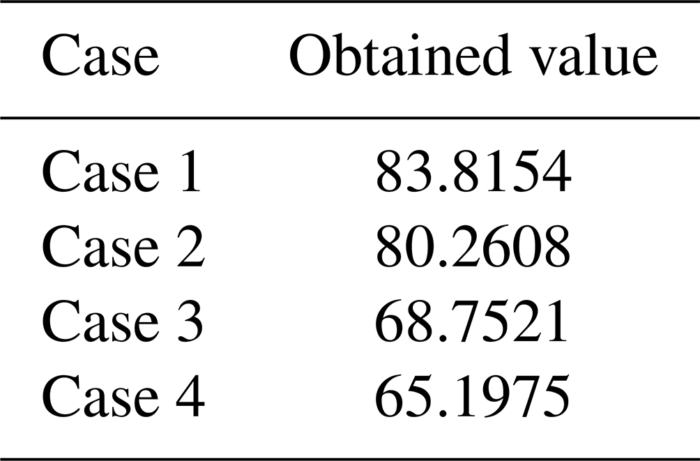
It can be seen that Case 1 has the largest value, and the value decreases as we go from Case 1 to Case 4. Thus, Case 1 is the closest to the optimal solution and Case 4 is the farthest. Note that Case 4 has both the modifications that are made in Cases 2 and 3 with respect to Case 1. Since there was a decrease in the value as we go from Case 1 to Case 2 and a decrease in the value from Case 1 to Case 3, the largest decrease in the value is seen as we go from Case 1 to Case 4.