3D wind observations with a compact mobile lidar based on tropo- and stratospheric aerosol backscatter

We present the first measurements of simultaneous horizontal and vertical winds using a new lidar system developed at the Leibniz Institute of Atmospheric Physics in Kühlungsborn, Germany (54.12° N, 11.77° E), for the concept of Vertical And Horizontal COverage by LIdars (VAHCOLI). We describe the technical details of a multi-field-of-view (MFOV) upgrade, which allows the measurement of wind dynamics in the transition region from microscale to mesoscale (10³–10⁴ m). The method was applied at the edge of a developing high-pressure region, covering altitudes between 3 and 25 km. Comparisons between the lidar measurements and data from the European Centre for Medium-Range Weather Forecasts (ECMWF) show excellent agreement for the meridional wind component along the north beam of the lidar, which is better than 0.30±0.33 m s⁻¹, while along the south beam, a higher deviation with $-\mathrm{0.93}\pm \mathrm{0.73}$ m s⁻¹ is observed. Measurements of vertical wind show a significant underestimation of this component by ECMWF. Comparison of Aeolus winds to the lidar winds projected to the Aeolus viewing direction shows good agreement, with results better than $-\mathrm{0.12}\pm \mathrm{3.31}$ m s⁻¹. The capability of the MFOV lidar to explore small-scale asymmetries in the wind field is shown by a comparison of the north and south field of view, where we observe a wind asymmetry in the meridional winds, which is also present in ECMWF but underestimated by a factor of approximately 4.

1 Introduction

Accurate and comprehensive measurements of wind profiles play a critical role in various atmospheric studies and applications, including numerical weather prediction (NWP) (Baker et al., 2014; Stoffelen et al., 2005). However, obtaining such measurements presents significant challenges. In situ measurements using anemometers mounted on towers or masts are limited to the boundary layer, whereas wind measurements from radiosondes, aeroplanes, and rockets can only offer snapshots of the winds and lack continuous coverage.

To achieve continuous wind measurements with a high degree of accuracy and spatiotemporal resolution, ground-based remote sensing methods are required. The most prominent ground-based techniques for measuring wind are sodar, radar, and lidar. Sodar and radar face limitations in their altitude coverage due to technical constraints. Sodar wind profilers reach heights of up to 2 km by scattering sound waves off turbulence (Bailey, 2000), while radar can measure the troposphere and in the upper mesosphere and lower thermosphere (MLT) due to the presence of available scattering targets. However, there exists a significant altitude gap in radar's capability to measure wind between 20 and 80 km (Hocking, 1997). Ground-based Doppler wind lidars (DWLs) are the only remote sensing instruments capable of providing continuous wind profiles from the troposphere to the MLT with high vertical and temporal resolution.

One challenge associated with Doppler wind lidars is their inherent complexity, necessitating ample laboratory space for emitters, detectors, and telescopes, as well as skilled operators. Presently, there are only six operational DWLs worldwide capable of measuring wind in the middle atmosphere. These installations are located at L'Observatoire de Haute-Provence (OHP) in France (44° N, 6° E) (Souprayen et al., 1999b, a); Observatoire de Physique de l'Atmosphère de la Réunion (OPAR) on La Reunion island (21° S, 55° E) (Ratynski et al., 2023); the Arctic Lidar Observatory for Middle Atmosphere Research (ALOMAR) in Norway (69° N, 16° E) (Baumgarten, 2010); the Leibniz Institute for Atmospheric Physics in Kühlungsborn, Germany (54° N, 12° E) (Gerding et al., 2023); and two mobile wind lidars in the Hefei region of China (approximately 32° N, 117° E) (Xia et al., 2012; Yan et al., 2017; Chen et al., 2023).

Space-based Doppler wind lidars provide the ability to obtain global wind profiles. The first satellite carrying such an instrument is the Atmospheric Dynamics Mission – Aeolus (Aeolus), which embarked on its mission in August 2018 and continued its measurements until May 2023. Aeolus orbits the Earth in a sun-synchronous, dusk/dawn orbit (inclination of 97°) at a height of 320 km (ESA, 2020). Winds are measured orthogonal to the flight direction at an angle of 35° off-nadir on the night side of the Earth. Along this field of view, the mission aimed to provide line-of-sight (LOS) winds from the ground up to the lower stratosphere (up to 30 km), with an altitude resolution of 250 m to 2 km and an altitude-dependent precision of 1 to 3 m s⁻¹ (Drinkwater et al., 2016). The actual error estimates during the operation were proved to be in the range of 4.1 to 4.4 m s⁻¹ (Rayleigh) and 1.9 to 3.0 m s⁻¹ (Mie) by Martin et al. (2021). Later validation campaigns showed even higher random errors due to the decreasing signal levels throughout the mission. Witschas et al. (2022) report a random error for Rayleigh clear winds of 5.5 to 7.1 m s⁻¹ in the altitude range from 0.5–10.5 km, and Ratynski et al. (2023) report an error between 5.37 and 6.49 m s⁻¹ in the altitude range up to 27 km.

The Atmospheric Laser Doppler Instrument (ALADIN) on board Aeolus used a frequency-tripled Nd:YAG laser operating at 355 nm and two distinct receiver channels. The first channel utilises coupled Fabry–Pérot interferometers to capture the Rayleigh scattering signal, while the second channel incorporates a Fizeau interferometer to detect the narrowband Mie scattering (Paffrath et al., 2009; Reitebuch et al., 2009).

Since the wind measurements presented in this work relies solely on Mie scattering to cover the altitude range between 3 and 25 km, a closer look at its use by the Aeolus satellite is valuable. Within the height range covered by Aeolus, the Rayleigh and Mie scattering techniques serve complementary purposes. In scenarios where the atmosphere is laden with significant aerosol loads, such as clouds or smoke plumes, the quality of the Rayleigh winds may be compromised. However, the Mie winds derived under these conditions exhibit exceptional quality, with error estimates approximately half of that associated with clean Rayleigh winds (Rennie et al., 2021; Rani et al., 2022).

This reduction in measurement error can be attributed to the narrowband nature of Mie scattering, which allows for a more accurate estimation of the Doppler shift. Due to the substantial mass of the aerosol scattering particles, temperature-induced broadening of the Mie backscattered signal can be neglected. As a result, the spectral width of the Mie scatter is about 2 orders of magnitude smaller than that of the Rayleigh scatter for Aeolus and about 3 orders of magnitude smaller for the instrument presented in this work.

While these advantageous spectral properties of Mie scattering enable more precise wind measurements, it is important to note that the ALADIN instrument requires complementary Rayleigh winds, since the use of the Mie channel necessitates sufficient aerosol loading to derive Mie winds. Consequently, it cannot solely rely on background aerosols present in the atmosphere for wind measurements (Drinkwater et al., 2016; Reitebuch et al., 2009). Other wind lidar instruments, like the ALADIN A2D Airborne Demonstrator, Ball Aerospace's airborne Green Optical Autocovariance Wind Lidar (OAWL), or heterodyne detection wind lidars in general, use Mie scattering to measure wind speeds covering mostly the troposphere (Lux et al., 2022; Baidar et al., 2018). However, as will be shown in the following sections, the lidar systems introduced in this work have the capacity to detect aerosols at up to 25 km that are invisible to ALADIN and use them for precise wind measurements. This capability is unique for ground-based instruments and makes a cluster of them especially interesting for intercomparison studies with upcoming Aeolus successors. Additionally, such a cluster or network will be especially interesting for the observation of atmospheric phenomena on horizontal and vertical scales which are inaccessible to other measurement techniques, as discussed in Lübken and Höffner (2021).

The organisation of this paper is as follows: Sect. 2 provides a technical overview of the lidar system, including its design, instrumentation, and key features. Section 3 describes a measurement campaign conducted from 16 to 18 December 2022, data collection procedures, and processing techniques. Section 4 presents the results of the wind measurements, including the vertical and horizontal wind profiles obtained and their comparison to data from the European Centre for Medium-Range Weather Forecasts (ECMWF) and Aeolus. Finally, Sect. 5 discusses the implications of the findings, highlights the contributions of this work, and suggests potential avenues for future research.

2 The lidar system

The lidar unit used in this work is called VAHCOLI 1. Figure 1 shows this instrument, along with a prototype system. VAHCOLI stands for Vertical And Horizontal COverage by LIdars and is a concept for lidars which encompasses a network of instruments to provide the horizontal coverage that lidars typically lack (Lübken and Höffner, 2021). For this reason, a new lidar system has been developed, which is small and mobile, yet designed to measure Doppler–Mie, Doppler–Rayleigh, and Doppler resonance scatter. The first prototype of this new lidar system (VAHCOLI 0) started operation in late 2019, and since then, two additional lidar systems have been constructed (VAHCOLI 1 and 2). In 2022, the capabilities of VAHCOLI 1 were significantly extended with a multi-field-of-view (MFOV) upgrade to provide a way to measure horizontal and vertical winds simultaneously. Though the general measurement principle of the VAHCOLI lidar has been developed based on the mobile potassium lidar of the Leibniz Institute of Atmospheric Physics (IAP), the measurement hardware has drastically improved in order to have such a compact system (von Zahn and Höffner, 1996; Fricke-Begemann et al., 2002; Höffner and Lübken, 2007).

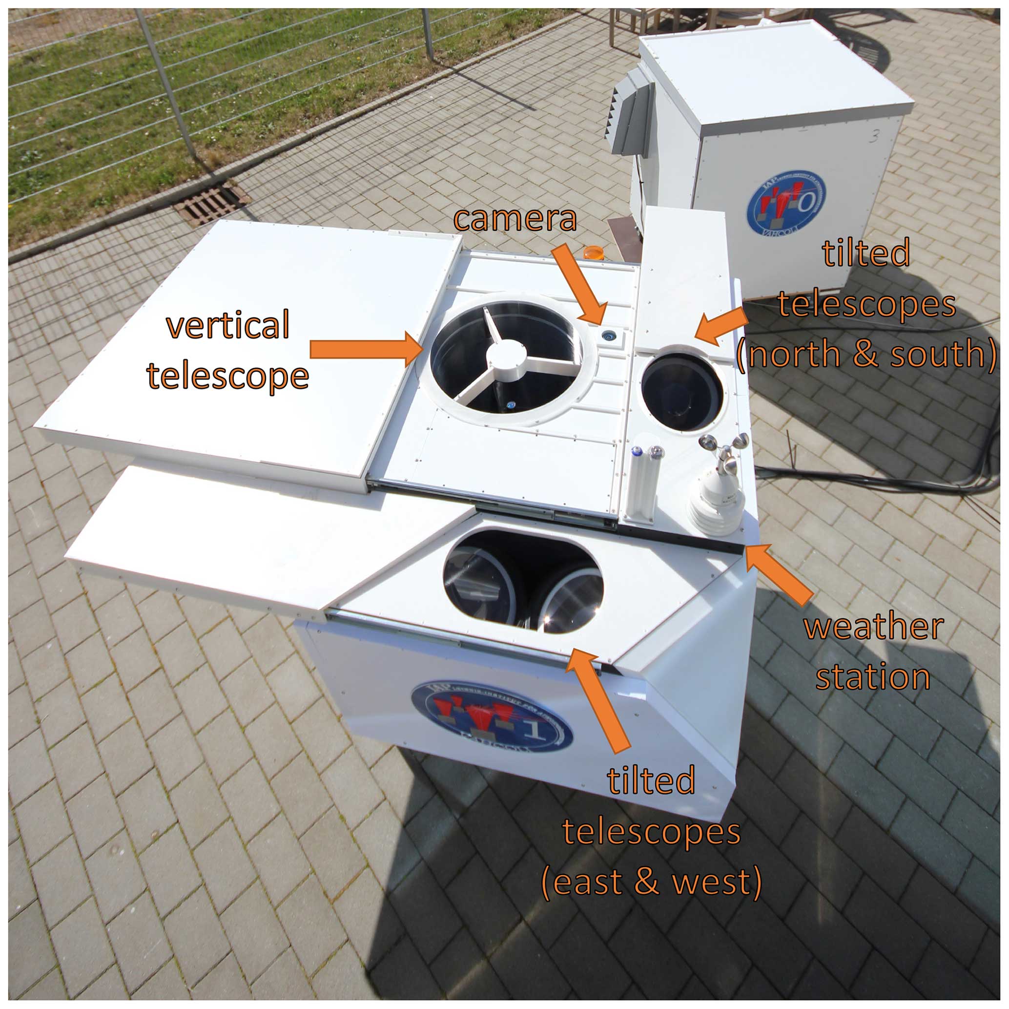
Figure 1 The upgraded VAHCOLI 1 lidar system on the testing ground in Kühlungsborn, Germany. The automatic hatches are open, revealing the 50 cm vertical-pointing mirror telescope visible in the centre of the core unit and the four additional lens telescopes mounted to two sides of the core unit. Other interesting features visible include the window for the vertical-pointing camera, next to the vertical telescope and the weather station in the corner of the MFOV upgrade. The prototype lidar unit (VAHCOLI 0), which can only measure vertically, is visible in the background (Lübken and Höffner, 2021).

2.1 The lidar core unit

The core unit of a VAHCOLI 1 comprises all the hardware necessary for fully autonomous measurements in a rugged, climate-controlled enclosure with a volume of roughly 1 m³. Figure 2 illustrates how this enclosure is built in modular layers that are 3D printed in-house, using large-scale FFF (fused-filament fabrication) printers. Likewise, the majority of the internal structural components are printed in-house. Layer 1 contains housekeeping hardware, power supplies for the system, a battery to buffer short power grid issues, and a custom industrial computer, which controls the whole system with three high-performance measurement cards. Layer 2 contains parts of the optical set-up, like the seeding laser, the diode pump, and a fibre resonator for reference, as well as the compact detection bench with its two avalanche photodiode (APD) detectors and stabilised filters. Layer 3 houses the emission part, with the biggest part being the diode-pumped Alexandrite ring laser, which was specially designed in close collaboration with the Fraunhofer Institute for Laser Technology in Aachen (Munk et al., 2021). The telescope cylinder, for the vertically facing 50 cm mirror telescope, passes through all layers.

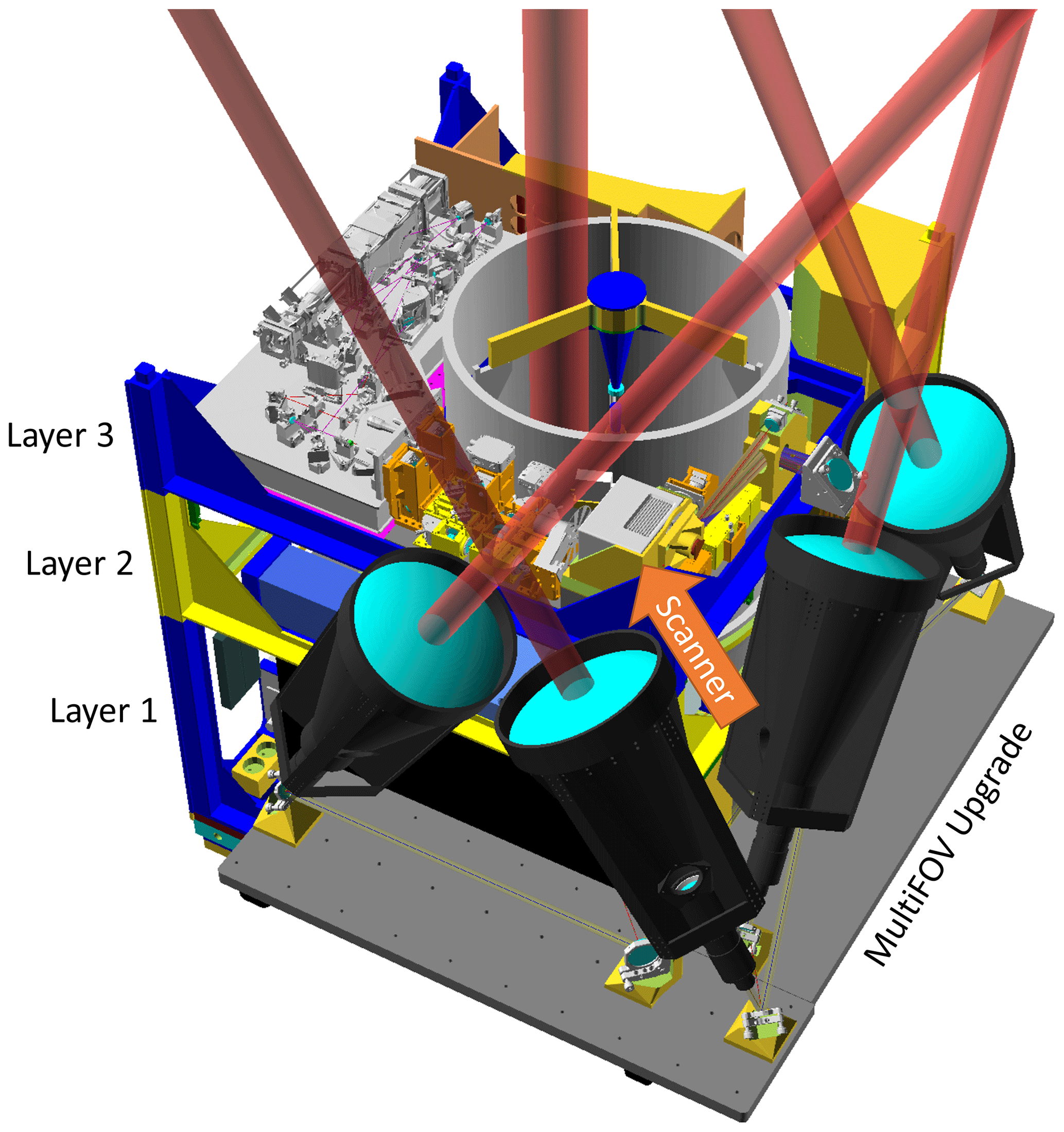
Figure 2 Computer-aided design (CAD) drawing of the new lidar unit equipped with multiple fields of view. A cubic metre core unit contains the measurement hardware of the lidar and a 50 cm vertically pointing mirror telescope, similar to the system described in Lübken and Höffner (2021). The optical set-up in the core unit has been extended by a two-axes galvanometer scanner, controlling the field of view. Four additional telescopes are mounted in an L-shaped extension mounted to the side of the system. The outgoing laser beams of the system are represented in red, and the three individual layers of the core unit are colour coded in blue and yellow.

Based on this hardware, the lidar can do high-resolution spectroscopy of the backscattered signal. For this reason, the frequency of the power laser is quickly and precisely scanned over two highly stabilised filters, a broadband solid etalon with a full width at half maximum (FWHM) close to the Doppler width of the atmospheric molecular line, and a narrowband confocal etalon (FWHM 7.5 MHz). Of the two APDs, one records the signal, which is transmitted through the planar and confocal etalon (APD1), and the other one records the signal, which is transmitted through the planar etalon but is reflected on the confocal etalon (APD2). The resulting spectra contain a mixture of Mie and Rayleigh backscatter on APD2 and mostly Mie backscatter on APD1, with a little bit (roughly $\mathrm{1}/\mathrm{60}$th) of Rayleigh backscatter as background. We derive atmospheric properties like wind and aerosol content from these measured spectra. A more detailed description of the core unit and the measurement technique can be found in Lübken and Höffner (2021), Froh (2021), and Munk et al. (2023).

2.2 The multi-field-of-view upgrade

In order to expand the capabilities of the core unit to measurements of horizontal winds, the system was upgraded with multiple fields of view (MFOV upgrade). While other Doppler lidars that measure at stratospheric altitudes use one telescope for each wind component, VAHCOLI 1 has four tilted telescopes that allow it to measure each horizontal component with two opposing fields of view (Khaykin et al., 2020; Baumgarten, 2010; Gerding et al., 2023). This allows the direct observation of gradients in the measured atmospheric parameters by the comparison of two fields of view.

The general optical set-up of the MFOV upgrade can be divided into a two-axes galvanometer scanner (inside the core unit) and an L-shaped enclosure holding the four additional telescopes, which is mounted to the walls of the core unit. In the core unit of VAHCOLI 1, the galvanometer scanner enables rapid switching between the five fields of view in shorter than 1 ms by rapidly rotating its two mirrors to preprogrammed positions.

The following specifications were met in the design of the four additional telescopes: (1) compact and relatively light design to keep the dimensions of the upgrade small and forces on the core unit low, (2) reasonable large aperture to measure up to the stratosphere, and (3) a cost-effective solution to allow for network construction as envisaged in VAHCOLI. Since no available telescopes on the market met these requirements, we developed them to the specifications we needed. We designed diffraction-limited lens telescopes with a clear aperture of the front lens of 200 mm, an overall length smaller than 600 mm, and a weight lighter than 5 kg. We use commercial off-the-shelf and 3D-printed components, allowing for fast and cost-effective integration of the MFOV upgrade. A challenge we faced in the telescope design was caused by the requirement to operate the system during night and day. This presented the risk of the telescopes pointing directly at the Sun, resulting in considerable thermal load. To overcome this obstacle, we implemented a robust cooling system and carefully selected materials that ensures that the telescopes are resilient in such circumstances. Four of these telescopes are held in the 3D-printed enclosure of the MFOV upgrade at a 30° off-zenith angle facing north, south, east, and west. The pointing precision of the telescopes is limited only by the precision of the 3D printer, since the enclosure and telescope mount are printed as one big part. From the dimensional accuracy and surface quality our 3D printers produce, we estimate the angular error introduced by the 3D-printed construction to be less than 2 mrad. A tilt sensor inside the core unit measures the level of the whole unit with a precision better than 0.1°, and an integrated camera can be used to additionally verify the instrument orientation using the stars with a precision better than 0.2°.

The MFOV upgrade drastically increases the capabilities, while the hardware upgrades were manageable. The high-speed two-axes scanner and the four extra fields of view, however, required significant upgrades to the control software.

3 The December 2022 campaign

The first campaign using VAHCOLI 1 with the MFOV upgrade took place in December 2022, namely from 16 December at 11:28 UT until 18 December at 12:10 UT.

3.1 Measurement conditions

To acquire the measurements presented in this publication, the VAHCOLI 1 instrument was placed outside on a paved and fenced-in area, with markings on the ground indicating true north direction. No further preparations of the site were required. The orientation of the system in the true north direction was verified by targeting Polaris. During the measurement, the local weather conditions were monitored by a weather station situated roughly 50 m away from the instrument. Over the course of the measurement, the air pressure increased from 1000 to 1024 hPa, the ground temperature was between −2 and −8 °C, and the relative humidity was high, with values ranging between 75 % and 100 %.

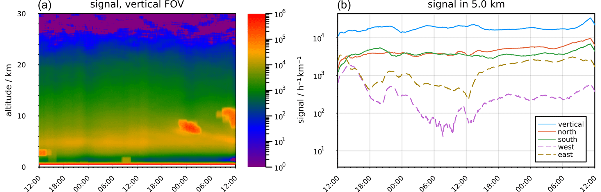
Figure 3 Backscatter signal of the vertical field of view (a) and backscatter signal at 5 km in each of the five fields of view (b) from 16 December 2022 at 12:00 UT to 18 December 2022 at 12:00 UT. The data are smoothed by the 2 h and 1 km integration window, which is shifted in 2 min and 100 m steps. The data are then converted to units of counts per time per altitude. The signal increase at approximately 7–11 km at 00:00 UT on 18 December is caused by the presence of cirrus clouds, which effectively improves the capability to measure winds with the lidar. Due to a larger aperture, the signal from the vertical FOV is generally larger compared to the horizontal FOVs.

At the beginning of the measurement, the signal strength of all four oblique fields of view was about a factor of 3 to 4 less than that of the vertical field of view (see Fig. 3). This is expected due to the smaller size of the lens telescopes. Over the course of the measurement, the signal in the meridional fields of view stayed almost constant, whereas the zonal fields of view experienced a sharp loss in signal strength. The signal decreased due to icing and condensation occurring on the two zonal-pointing telescopes, caused by the cold temperatures and high relative humidity. An internal heating element was switched on for de-icing at around 12:00 UT on 17 December, leading to an increase in the signal of both telescopes. The signal in the westward-pointing telescope only recovered to 13 % of its initial value. As a result, our westward zonal winds have a lower top altitude than our eastward zonal winds, and both have a significantly reduced performance with more data gaps compared to the meridional telescopes. During this measurement, the planar etalon discussed in Sect. 2.1 was not installed, leading to a slight increase in the daylight background. Despite this, no significant performance drops connected to this daylight background were observed.

Except for the icing problem, the system and the MFOV upgrade performed well, with no major problems or interruptions, even under these harsh winter conditions close to the Baltic Sea. After this initial measurement campaign, the VAHCOLI 1 system remained in operation and, as of June 2023, has accumulated more than 600 h of measurements, of which 85 h were done in MFOV mode.

3.2 Retrieval of horizontal and vertical winds from the lidar data

VAHCOLI is a frequency-scanning lidar, which measures the spectra of the backscattered signal (Höffner et al., 2021; Lübken and Höffner, 2021). For the measurements presented in this publication, the Mie channel of the system has been used. Mie scattering provides the best wind measurements up to 25 km, due to its very narrow spectrum, but is limited in the lower stratosphere by the decreasing concentration of aerosols. Typically above 25 km, the aerosol density drastically drops, giving an upper altitude limit for the use of this method.

For data processing the individual pulse raw data, produced by the system with a time resolution of 2 ms and an electronic altitude resolution of 1 m, are first converted to backscatter spectra with an integration time of 2 min and a height resolution of 1 m for each individual field of view. The laser pulse itself has a length of approximately 165 m (full width at half maximum) in the atmosphere. In order to improve the statistics for the analysis, these spectra are then integrated in time and altitude with a floating window to the wanted final resolutions of the data. Unless stated otherwise, an integration window of 2 h and 1000 m is used, which is moved in 2 min and 100 m steps. Winds are derived from the Mie backscatter spectra by fitting a Voigt function to each height channel, with an example of this fit shown in Fig. 4. The laser's spectral shape was determined to be a Voigt function through lab measurements, which will be detailed in an upcoming publication. The detection filter employed for Mie scattering is a confocal etalon, which has a Lorentzian filter curve. The atmospheric broadening, corresponding to wind fluctuations, is assumed to follow a Gaussian distribution. Hence, the convolution of a Voigt function, a Lorentzian function, and a Gaussian function yields another Voigt function.

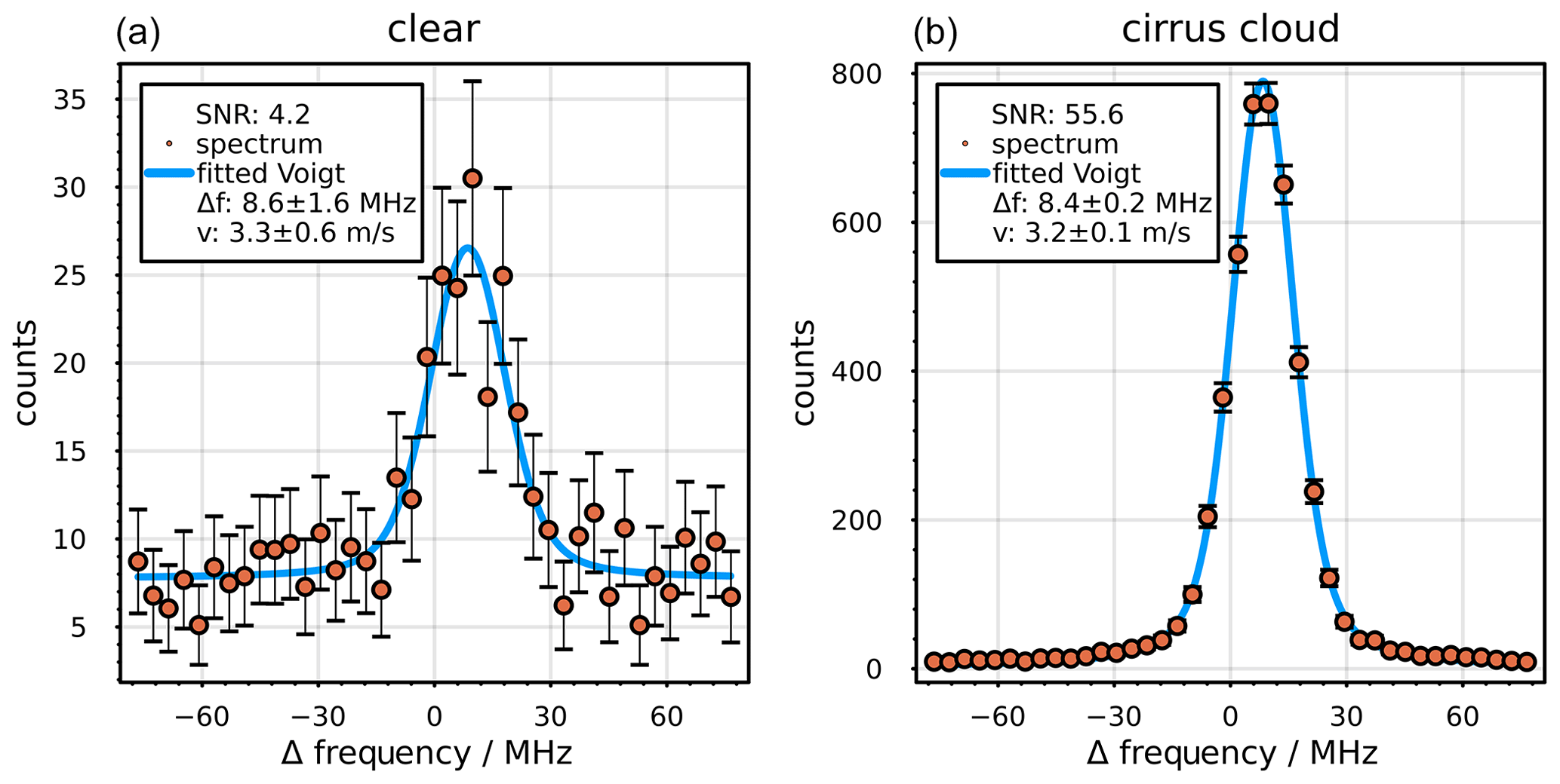
Figure 4 Example of the spectrum measured from 9.25 to 10.25 km, with an integration time of 20 min in the north field of view, together with the fitted Voigt function in clear air (a) and in cirrus cloud (b). Corresponding signal-to-noise ratios ($\mathrm{SNR}=\mathrm{PeakSignal}/\mathrm{Background}$) and errors in frequency offset and winds derived from the fits are shown in the inlets.

From the Doppler shift, Δf, given by fitting a Voigt function to the measured spectra, the line-of-sight wind can be derived by rearranging the Doppler shift equation to $v_{\mathrm{LOS}}=\mathrm{\Delta }f/\left(\mathrm{2}{f}_{\mathrm{0}}\right)\cdot c$ with c the speed of light and f₀ the fundamental frequency (e.g. the laser frequency). Since we measure both the vertical and four off-zenith line-of-sight winds simultaneously, the vertical component can be immediately removed to derive horizontal wind components. The horizontal winds must be divided by sin (30°) to compensate for the off-zenith tilt. It is important to note that this technique is based on a relative measurement of the Doppler shift. This is done by comparing the measured backscatter spectrum to the reference spectrum within the system, as described by Lübken and Höffner (2021). Due to the design of the instrument as a resonance lidar, the exact laser wavelength of 769.898 nm is known from the usage of potassium saturation spectroscopy as an absolute wavelength reference, even though the Mie–Doppler measurements do not strictly require this precise knowledge of it.

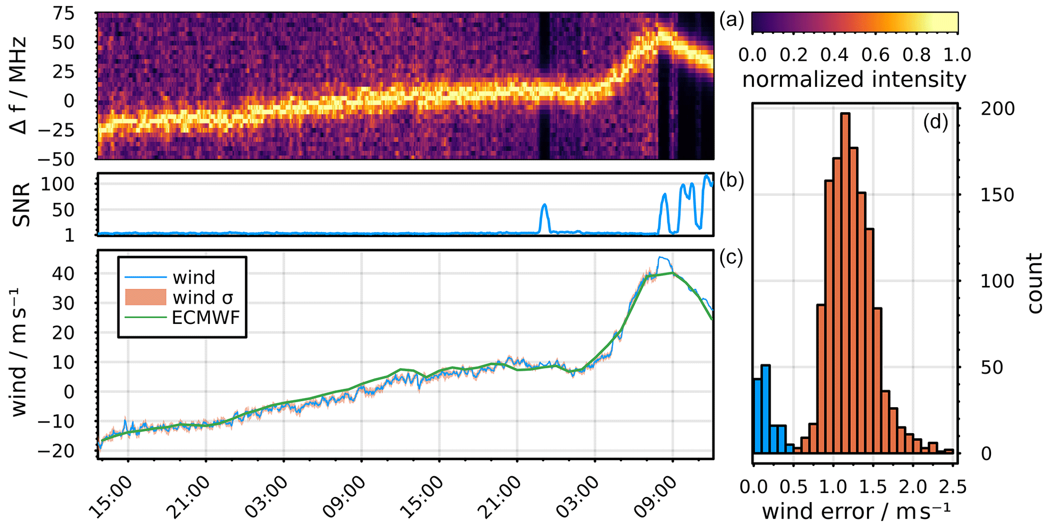
Figure 5 Connection between measured spectra, calculated wind, and wind error. (a) Example of an atmospheric spectrum measured between 16 and 18 December 2022 with the north-facing telescope integrated from 9.25 to 10.25 km, a gridded time resolution of 2 min, and an integration time of 20 min. The purple and black regions in the spectrum plot represent the lidar background. The black corresponds to the cirrus clouds seen in Fig. 3 which result in a higher signal-to-noise ratio (SNR) value. (b) SNR calculated from the spectrum above. (c) Calculated lidar average wind speed (blue) together with the wind error estimate (orange ribbon), which is at the line strength of the wind speed most of the time. The corresponding ECMWF Integrated Forecasting System (IFS) wind time series is shown for reference (green). A significant deviation in the measured wind and the ECMWF wind is visible on 18 December at around 08:00 UT, probably caused by the much higher smoothing in ECMWF. (d) Histogram of the error estimate for the wind from measurements with high (blue) and low (orange) aerosol loading.

The error estimate for the LOS winds (σ_Δv) is derived from the error estimate of the Doppler shift (σ_Δf), using the propagation of uncertainties (${\mathit{\sigma }}_{\mathrm{\Delta }v}={\mathit{\sigma }}_{\mathrm{\Delta }f}\cdot c/\left(\mathrm{2}{f}_{\mathrm{0}}\right)$). σ_Δf is a product of the fit routine, which uses the least square fitting of the spectrum, with the standard deviation of each fit parameter being the square root of the corresponding diagonal element of the covariance matrix (Hansen et al., 2013). This requires an estimate of the error in the photon counts (n) in each frequency bin of the spectrum. Here we assume a Poisson distribution with a width of ${\mathit{\sigma }}_n=\sqrt{n}$. The precision of the result of the fit benefits from the very narrow spectral shape of the received Mie signal and its high-edge steepness, which facilitates precise determination of the Doppler shift. Together with the suppression of the background Rayleigh signal, the number of needed photons is significantly reduced to achieve acceptable wind errors compared to traditional DWL systems (Höffner et al., 2021). Figure 5 shows this connection between the measured spectrum of the Mie scattering, the calculated LOS wind, and the error estimate. A change in the peak position in the measured spectrum results in a change in the wind. Black lines in the background of the spectrum correspond to the presence of cirrus clouds, which significantly increase the signal to noise ratio of the spectrum and thus reduce the calculated error in the measurement. This leads to a double distribution of the wind error visible in the bottom right of Fig. 5, with one peak around 0.15 m s⁻¹ produced by measurements with cirrus clouds and one peak around 1.15 m s⁻¹ from measurements without cirrus clouds. Figure 4 shows an example of each of these cases. The clear-air case shows a low signal-to-noise (SNR) ratio of 4.2, resulting in an error estimate of the Doppler shift of 1.6 MHz and thus a wind error of 0.6 m s⁻¹. In the case of a cirrus cloud, the SNR drastically increases by more than an order of magnitude, resulting in an error estimate of the Doppler shift of 0.2 MHz and thus a wind error of less than 0.1 m s⁻¹. In cirrus clouds and other strong aerosol loads, the integration in time and altitude can be significantly reduced while maintaining wind errors below 1 m s⁻¹.

3.3 ECMWF and Aeolus winds

In this work, we utilised the ECMWF winds in two distinct approaches. First, we directly employed the ECMWF winds interpolated to the instrument's location (see Figs. 6, 7, and 8). Second, to achieve a more comprehensive comparison with the individual fields of view, we interpolated and sampled the ECMWF winds along simulated beams (see Figs. 5, 9, and 10). This interpolation and sampling process is very important due to the increasing positional difference between the beams at higher measurement altitudes. At a height of 20 km, the separation between two opposite fields of view reaches 23 km, exceeding the ECMWF horizontal resolution of about 9 km. In both cases, an observational filter is applied to match the lidar altitude and time resolution.

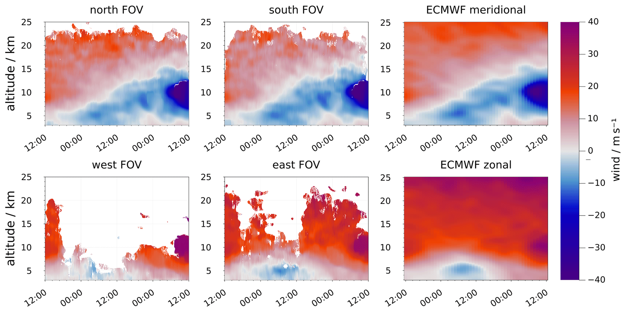
Figure 6 Horizontal winds measured between 16 December at 12:00 UT and 18 December at 12:00 UT in the in the north, south, west, and east fields of view (see plot titles), using a vertical integration of 1000 m and an integration time of 2 h. The corresponding meridional and zonal winds from ECMWF are shown in the two right-most panels. The integration window was shifted in 100 m and 2 min steps. Winds with a LOS wind error of more than 2 m s⁻¹ are masked. The LOS winds of the tilted telescopes are converted to zonal and meridional winds. In the meridional winds, a clear transition around the tropopause from mainly southward winds at the beginning of the measurement to strong northward winds at the end is visible. The lower signal strength in the zonal FOVs causes some gaps in the wind retrieval, affecting especially the higher altitudes.

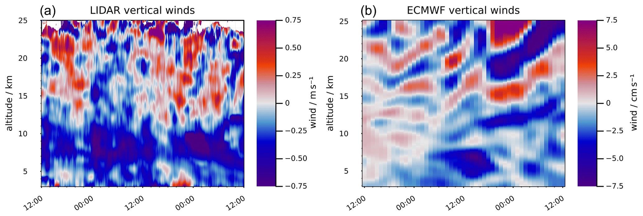
Figure 7 Measured vertical winds (a) and the corresponding vertical winds from the ECMWF (b). The vertical winds in ECMWF are underestimated by approximately an order of magnitude. In the upper troposphere, a constant background flow of descending air can be observed in the measured winds.

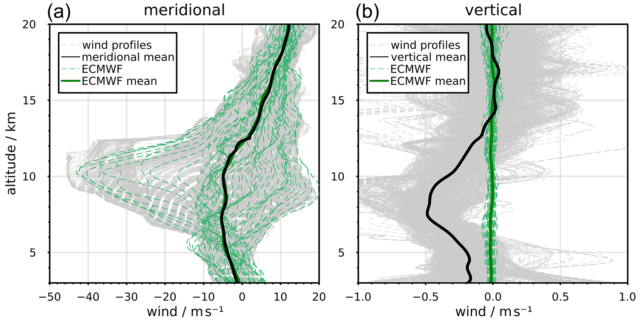
Figure 8 Meridional (a) and vertical (b) wind profiles measured (dashed grey lines), together with the calculated mean (thick black line), from 16 December at 12:00 UT to 18 December at 12:00 UT, with the individual wind profiles from the ECMWF data set (dashed green lines), and the time-averaged ECMWF wind profile (thick green line). The individual wind profiles indicate the variability in the wind during the measurement period, with the highest variability in the meridional winds around the tropopause region.

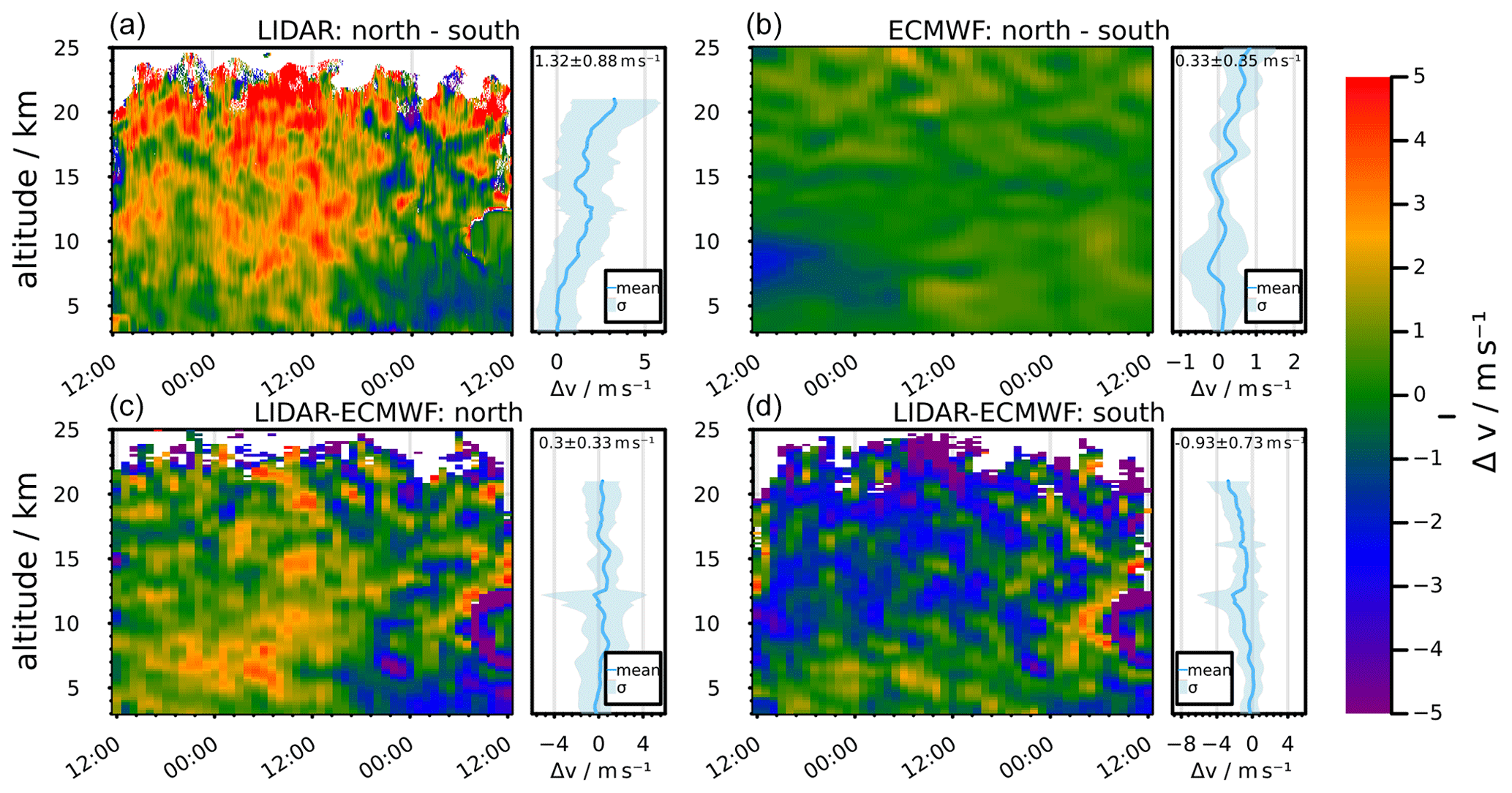
Figure 9 Difference in the meridional winds (Δv) in the time from 16 December at 12:00 UT to 18 December at 12:00 UT between 3 and 25 km, together with the altitude-dependent mean and standard deviation. (a) Difference between the north and south field of view of the lidar ($\mathrm{\Delta }v=v_{\mathrm{lidar},\mathrm{north}}-v_{\mathrm{lidar},\mathrm{south}}$). (b) Difference between the ECMWF meridional winds sampled along the north and the south FOV ($\mathrm{\Delta }v=v_{\mathrm{ecmwf},\mathrm{north}}-v_{\mathrm{ecmwf},\mathrm{south}}$). (c) Difference between meridional winds measured along the north FOV of the lidar and the ECMWF winds sampled along the north FOV ($\mathrm{\Delta }v=v_{\mathrm{lidar},\mathrm{north}}-v_{\mathrm{ecmwf},\mathrm{north}}$). (d) Same as the bottom left but for the south FOV ($\mathrm{\Delta }v=v_{\mathrm{lidar},\mathrm{south}}-v_{\mathrm{ecmwf},\mathrm{south}}$). The altitude-dependent mean and standard deviation have only been calculated up to 21 km when using lidar data to avoid the influence of gappy data. For every difference, the column mean and its standard deviation have been calculated. In the lidar measurement, we see a much stronger difference between the north and south field of view than in ECMWF.

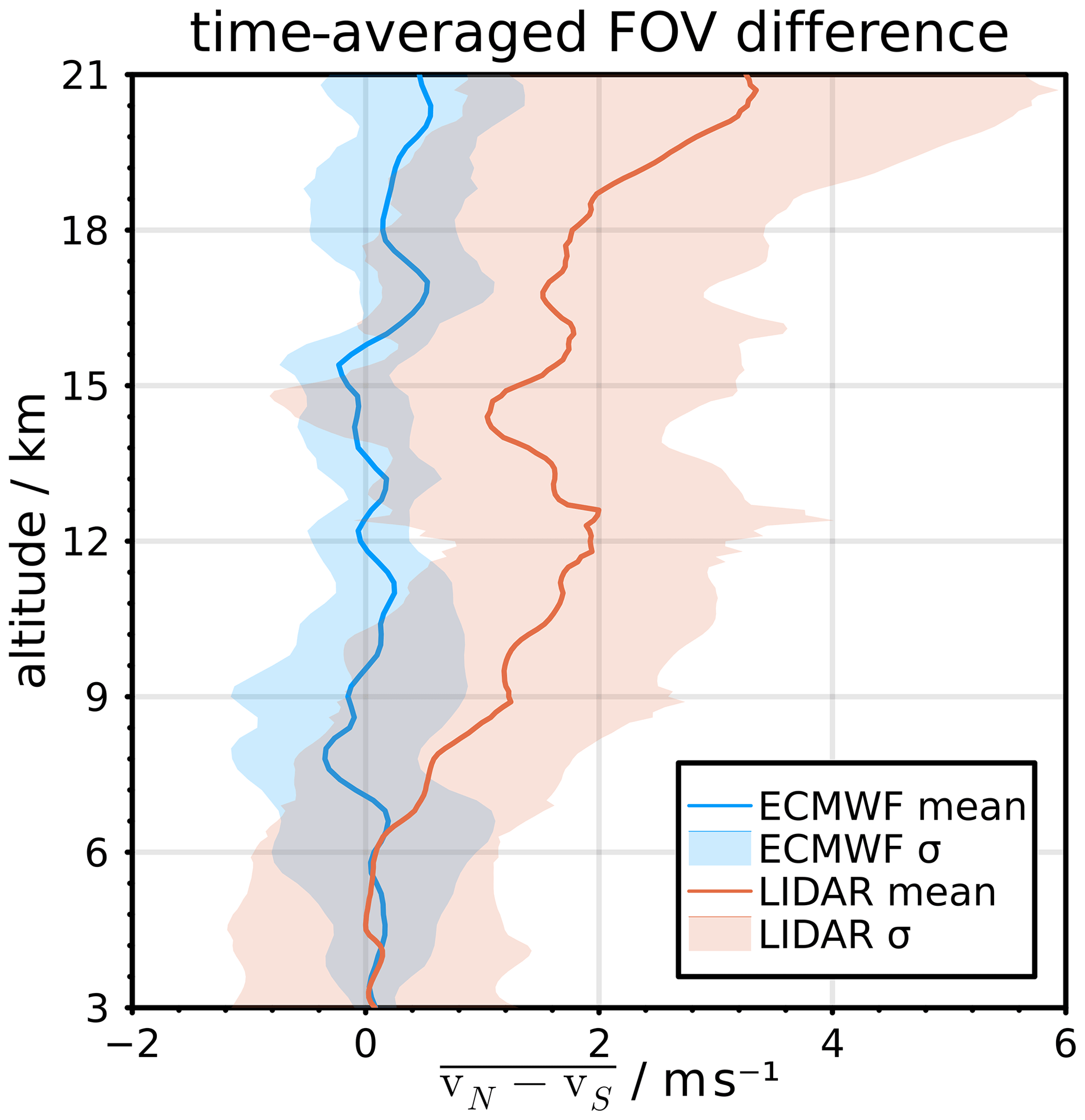
Figure 10 Comparison of the time-averaged differences between the north and the south field of view of the lidar measurements and the ECMWF winds sampled along the two fields of view. The time average is taken between 16 December at 12:00 UT and 18 December at 12:00 UT. The blue and orange lines represent the mean difference, and the corresponding shading is the standard deviation. The lidar measurement shows a strong altitude dependency, which is caused by an asymmetry in the measured meridional winds in the north and south field of view.

The Aeolus data have been reprocessed using the baseline 2B15 and regridded to an altitude resolution of 1 km, as in Banyard et al. (2021). Only Rayleigh clear winds are used, due to the scarcity of Mie cloudy winds. It is worth noting here that Aeolus winds and ECMWF winds are not really independent, since Aeolus data were assimilated into the ECMWF model.

4 Results

4.1 Horizontal winds

The horizontal winds from all four off-zenith lidar directions are shown in Fig. 6, as well as the corresponding wind time series from the ECMWF Integrated Forecast System (ECMWF IFS) interpolated to the location of the lidar. In the meridional wind, a drastic change during the measurement is observed, which corresponds to small-scale wind variations associated with the edge of a developing high-pressure region, which is visible in weather maps of this time period. While the meridional winds above 5 km are between 10 and 20 m s⁻¹ (northward) at the beginning of the measurement, a wind reversal in the tropopause region is observed, with the winds exceeding −40 m s⁻¹ (southward).

In the zonal winds, the previously discussed signal losses are clearly visible as gaps in the top measurement height. Despite the gaps, it was still possible to retrieve zonal wind up to 15 km​​​​​​​ or higher using the eastward-facing telescope during the majority of the measurement. Here the wind peak in the tropopause region is also visible at the end of the measurement, with winds reaching 40 m s⁻¹.

A first qualitative comparison to the winds from ECMWF IFS shows the same features in zonal and meridional winds with similar amplitudes. A more quantitative comparison can be found in Sect. 4.3.

4.2 Vertical winds

The vertical winds measured are shown in Fig. 7. Overall, the measured vertical winds show absolute wind speeds of 1 m s⁻¹ or slower, with a clear separation in the behaviour between the troposphere and the stratosphere. While above 11 km the winds fluctuate around zero, presumably due to the passage of gravity waves, below a constant background flow of descending air can be observed. A possible influence of the horizontal winds due to pointing errors will be discussed later in Sect. 5. When comparing the measured vertical winds with vertical winds from ECMWF, differences are immediately apparent. ECMWF underestimates the vertical wind fluctuations by approximately an order of magnitude, which is especially visible in the stratosphere. Additionally, ECMWF does not show the same clear separation between the troposphere and stratosphere.

4.3 Comparison of lidar winds with ECMWF and Aeolus

The comparison of the mean winds during the measurement with the time-averaged ECMWF data over the 48 h of the measurement (see Fig. 8) shows the good agreement of the ECMWF data with the measurement in the meridional direction.

The qualitative comparison presented in Fig. 6 shows that the wind pattern observed is similar to the ECMWF zonal wind pattern. In the vertical winds, the behaviour discussed in Sect. 4.2 is clearly visible, with downward winds in the lower part of the measurements. The comparison of the meridional winds measured along the north and south field of view (see Fig. 9, top left) shows a systematic difference between the two fields of view, with the winds in the north field of view being larger than in the south field of view. This effect increases with altitude. The column mean of the time-averaged difference is 1.32 m s⁻¹, with a standard deviation of 0.88 m s⁻¹. The same analysis of the interpolated and beam-sampled ECMWF winds shows a similar trend, but much less pronounced (see Fig. 9, top right), with a column mean of the time-averaged difference of 0.33 m s⁻¹​​​​​​​ and a standard deviation of 0.35 m s⁻¹.

The direct comparison of the time-averaged field of view difference in Fig. 10 highlights this. In both the lidar measurements and the ECMWF data, differences in similar altitude dependency are visible, but the difference between the north and south field of view is much more pronounced in the lidar measurements.

The comparison of the meridional winds from the lidar measurement and ECMWF along the individual fields of view (see Fig. 9, bottom) paints a similar picture. Along the north field of view, the meridional winds measured with the lidar are slightly higher on average than the winds in ECMWF but show excellent agreement in general. The column mean of the difference between lidar and ECMWF winds in the north field of view is 0.30 m s⁻¹, with a standard deviation of 0.33 m s⁻¹. Along the south field of view, the lidar-measured winds are on average lower than the ECMWF winds, with a column average of −0.93 m s⁻¹ and a standard deviation of 0.73 m s⁻¹, and differences are more pronounced in the time-resolved heatmap. Especially in the stratosphere, the differences show an altitude dependence associated with the increase in horizontal distance between the fields of view with altitude. Around the tropopause region, significant deviations are also observable.

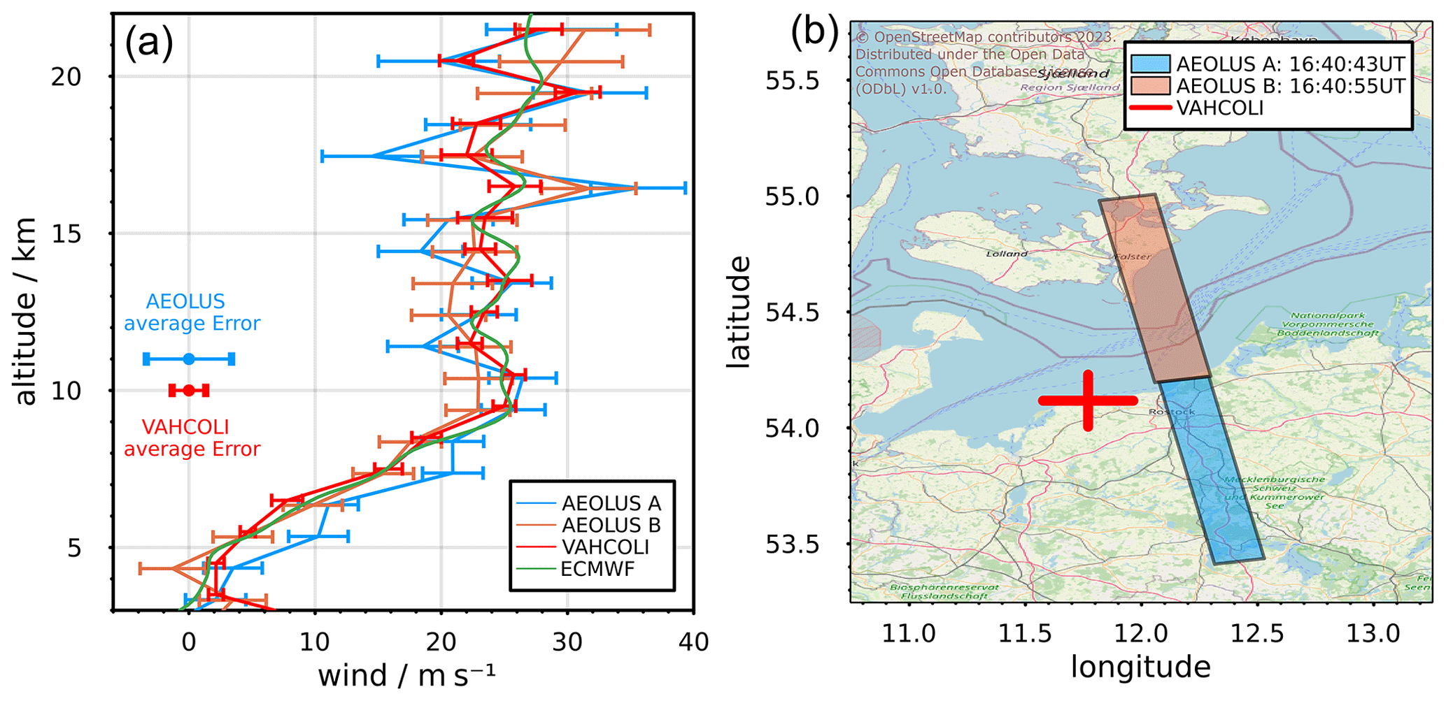
Figure 11 (a) Comparison of Rayleigh clear winds measured by Aeolus (blue and orange lines) and Mie winds measured by the VAHCOLI 1 lidar system (red lines), together with the winds from ECMWF (green line). For winds from VAHCOLI and ECMWF, the meridional, zonal, and vertical components have been combined and projected on to the horizontal line of sight (HLOS) of Aeolus. The difference in the lidar measurement and the B profile from Aeolus is $-\mathrm{0.12}\pm \mathrm{3.31}$ m s⁻¹ on average, with the best agreement below 15 km. Additionally, the average errors for the VAHCOLI winds (1.3 m s⁻¹, red) and the Aeolus winds (3.3 m s⁻¹, blue) are marked. (b) Map showing the integration areas for the two Aeolus profiles (orange and blue boxes), together with the VAHCOLI beams (red lines) up to a height of 25 km. (Map: © OpenStreetMap contributors 2023. Distributed under the Open Data Commons Open Database License (ODbL) v1.0.).

For an additional comparison to a Doppler wind lidar, we used measurements from the Aeolus satellite. The closest overpass occurred on 16 December 2022 at 16:40:55 UT (over the coordinates 54.615° N, 12.1785° E), approximately 64 km from the VAHCOLI test site. For the comparison, the VAHCOLI measurements were downsampled with an altitude resolution of 1 km by 2 h integration time to match the altitude resolution of Aeolus. The measured wind components were combined and projected to the horizontal line of sight (HLOS) of Aeolus. The distance between the Aeolus position and the location of VAHCOLI 1 has been compensated by a time lag of 96 min, based on the observed drift of wind features through the multiple field of view of the VAHCOLI instrument. The comparison (see Fig. 11) shows good agreement between the projection of the Aeolus HLOS measurement and the projection of the VAHCOLI measurements. Using the 16:40:55 UT profile from Aeolus for a statistical analysis of the deviation like before results in a standard deviation of 3.31 m s⁻¹ and a mean deviation of −0.12 m s⁻¹, with the biggest differences occurring in the stratosphere. The average error estimate of 1.3 m s⁻¹ for the projected VAHCOLI wind is a factor of 2.5 lower than the average error estimate of 3.3 m s⁻¹ for the Aeolus HLOS wind.

5 Discussion

The lidar measurements during the period from 16 December 2022 at 12:00 UT to 18 December 2022 at 12:00 UT, were successful with the system operating for more than 48 h. The measured winds in the two meridional fields of view show the same wind pattern. The same is true for the zonal fields of view, despite the gaps in altitude coverage. The vertical-pointing accuracy of the system is estimated to be better than 0.5°, based on the internal sensor and the accuracy of the 3D-printed construction. Due to this and the narrow field of view (< 30 mrad), we rule out a contamination of the vertical wind by the horizontal wind components. This is supported by the winds in the stratosphere above 13 km, which are zero on average.

Although the measured horizontal winds show a convincing similarity to the winds reported by ECMWF both qualitatively and quantitatively, we observe a significant asymmetry of the wind field in meridional direction, which is not well represented in ECMWF. The effect is too large to be caused by a pointing error, since for a wind difference in this magnitude between the fields of view, a tilting error of 6° is required, which is much larger than our estimated tilting precision of 0.5°. More likely, we are observing a true gradient in the wind field above the lidar that is associated with the small-scale dynamics at the edge of a developing high-pressure region. ECMWF maps of the meridional wind for the period indicate the presence of such a gradient. We conclude that the ECMWF model is underestimating the gradient in the wind field due to its 9 km grid spacing. This highlights the importance of the MFOV Doppler lidar to measure these variations in the transition region between mesoscale and microscale (10³–10⁴ m horizontally). The assimilation of higher quality, real-time wind measurements, as provided by a network of ground-based lidar systems, will presumably improve the forecast capabilities of high-resolution numerical weather prediction models by providing information about these typically inaccessible small-scale processes.

Vertically, there are significant differences between measured and ECMWF winds, with higher fluctuations and systematic deviations, especially in the troposphere. As discussed before, it is not likely that a contamination of the vertical winds by the horizontal winds is the cause for these systematic deviations. Additionally, the negative vertical winds in the troposphere are in agreement with the increase in air pressure measured at ground level, as discussed in Sect. 3.1. The larger fluctuations in the vertical wind measurements are expected, since the lidar measurement volume is much smaller than the model cell size (about 9 km × 9 km in this case) and thus captures smaller-scale dynamics that are not captured in the model. The different sizes of the sounding volume and the model volume might also explain other differences between the measured data and ECMWF data. This underestimation of vertical wind speeds in ECMWF has also been previously reported and discussed (Preusse et al., 2014).

A comparison to one profile of Aeolus winds shows a good agreement to our measurements with an average deviation of $-\mathrm{0.12}\pm \mathrm{3.31}$ m s⁻¹. These values are well within the values discussed previously by Martin et al. (2021) for the Aeolus measurements. In general, the aerosol-based wind profiles from the VAHCOLI 1 instrument cover a larger altitude range than the Rayleigh winds from Aeolus. The VAHCOLI instruments have been purposefully designed to integrate seamlessly into a European lidar network in the foreseeable future. Even though the IAP goal for this network is to observe crucial dynamical processes in the middle atmosphere, such as gravity waves and stratified turbulence with sufficient temporal, vertical, and horizontal sampling and resolution, it is also exceptionally well suited to complementing the forthcoming Aeolus successor missions (Lübken and Höffner, 2021). While the satellites acquire top-down measurements and sample multiple locations sparsely, the VAHCOLI instruments adopt a Eulerian reference frame, observing the atmosphere from the ground up and offering continuous measurements. The assimilation of both the global wind measurements from satellites and the ground-based lidar network measurements into forecast models such as ECMWF promises significant enhancements to their capabilities, owing to the inherent complementarity of these data sets.

6 Conclusions

In this study, we present the very first measurements of winds along five fields of view covering the upper troposphere–lower stratosphere with a lidar. To our knowledge, all previous Doppler wind lidars reaching this altitude used three fields of view at most. The VAHCOLI instrument with the MFOV upgrade can provide continuous measurements of wind using backscatter from tropospheric and stratospheric aerosol from 3 up to 25 km in unattended and automated operation, even under challenging weather conditions.

Using the five fields of view of the instrument, we are capable of measuring small-scale wind asymmetry associated with the development of a high-pressure region in real time. We can access the transition region from micro- to mesoscale at horizontal wavelengths between 10³ and 10⁴ m. Assimilation of real-time observations from a network of Doppler wind lidars with these capabilities would be useful for the improvement of short-term weather forecast skills by resolving quickly evolving weather features.

We have achieved accurate real-time measurements of vertical wind and have shown that ECMWF underestimates the vertical wind by an order of magnitude during our case study. Our meridional winds were verified against ECMWF with an excellent agreement, with values better than 0.30±0.36 m s⁻¹ along the north beam of the lidar and $-\mathrm{0.93}\pm \mathrm{0.73}$ m s⁻¹ along the south beam.

We have found a good agreement with a measurement from an Aeolus overpass, with values better than $-\mathrm{0.12}\pm \mathrm{3.31}$ m s⁻¹, indicating that the data reliability of both systems is comparable. We envisage the addition of Rayleigh winds and temperatures to the lidar unit in the near future.