A cloud-by-cloud approach for studying aerosol–cloud interaction in satellite observations

The effective radiative forcing (ERF) due to aerosol–cloud interactions (ACIs) and rapid adjustments (ERFaci) still causes the largest uncertainty in the assessment of climate change. It is understood only with medium confidence and is studied primarily for warm clouds. Here, we present a novel cloud-by-cloud (C×C) approach for studying ACI in satellite observations that combines the concentration of cloud condensation nuclei (n_CCN) and ice nucleating particles (n_INP) from polar-orbiting lidar measurements with the development of the properties of individual clouds by tracking them in geostationary observations. We present a step-by-step description for obtaining matched aerosol–cloud cases. The application to satellite observations over central Europe and northern Africa during 2014, together with rigorous quality assurance, leads to 399 liquid-only clouds and 95 ice-containing clouds that can be matched to surrounding n_CCN and n_INP respectively at cloud level. We use this initial data set for assessing the impact of changes in cloud-relevant aerosol concentrations on the cloud droplet number concentration (N_d) and effective radius (r_eff) of liquid clouds and the phase of clouds in the regime of heterogeneous ice formation. We find a $\mathrm{\Delta }\ln N_{\text{d}}/\mathrm{\Delta }\ln n_{\text{CCN}}$ of 0.13 to 0.30, which is at the lower end of commonly inferred values of 0.3 to 0.8. The $\mathrm{\Delta }\ln r_{\text{eff}}/\mathrm{\Delta }\ln n_{\text{CCN}}$ between −0.09 and −0.21 suggests that r_eff decreases by −0.81 to −3.78 nm per increase in n_CCN of 1 cm⁻³. We also find a tendency towards more cloud ice and more fully glaciated clouds with increasing n_INP that cannot be explained by the increasingly lower cloud top temperature of supercooled-liquid, mixed-phase, and fully glaciated clouds alone. Applied to a larger number of observations, the C×C approach has the potential to enable the systematic investigation of warm and cold clouds. This marks a step change in the quantification of ERFaci from space.

1 Introduction

The optical and microphysical properties of clouds depend on the presence of atmospheric aerosol particles. Aerosols facilitate the formation of cloud droplets by acting as cloud condensation nuclei (CCN; Quinn et al., 2008). They also affect supercooled-liquid and ice-containing clouds by acting as ice nucleating particles (INPs; Kanji et al., 2017). Changes in the number of aerosols that can act as CCN and INPs through natural and anthropogenic emissions therefore influence the properties and the life cycle of clouds through aerosol–cloud interactions (ACIs) and the accompanying rapid adjustments. The resulting effective radiative forcing (ERF; Boucher et al., 2013) due to ACI (ERFaci) of $-\mathrm{1.0}\pm \mathrm{0.7}$ W m⁻² is still assessed with only medium confidence and marks the largest uncertainty in our understanding of anthropogenic changes to the Earth’s energy budget (Forster et al., 2021).

ACI can be distinguished for warm (liquid-water) and cold (mixed-phase and ice) clouds. The ERFaci in warm clouds is defined as the disturbance in short- and long-wave radiation due to a change in cloud droplet number concentration (N_d) triggered by a change in aerosol concentration (Bellouin et al., 2020; Quaas et al., 2020). ERFaci consists of (i) the instantaneous radiative forcing (IRFaci) related to the brightening of clouds in polluted environments (cloud albedo or Twomey effect; Twomey, 1974) and (ii) the rapid adjustments of cloud fraction f, liquid water path L, and cloud top temperature T_top (Albrecht, 1989; Ackerman et al., 2004) in prompt reaction to the perturbation of the Twomey effect. The challenge lies in quantifying (i) the sign of the combined adjustments (Mülmenstädt and Feingold, 2018; Gryspeerdt et al., 2019) and (ii) the anthropogenic contribution to the disturbance in aerosol concentration.

So far, the Twomey effect has been studied most extensively. Other proposed ACI mechanisms suggest that smaller droplets in non-precipitating clouds can be transported to larger heights, where they release latent heat for a stronger development of convective clouds (cloud invigoration effect; Rosenfeld et al., 2008) or delay cloud glaciation (thermodynamic effect; Lohmann and Feichter, 2005). At the same time, increased numbers of aerosols that can act as INPs might lead to an earlier onset of cloud glaciation which increases the precipitation efficiency of the clouds (glaciation effect; Lohmann, 2002). Depending on the types of aerosols and clouds, their interaction might either decrease or increase the susceptibility of clouds to form rain (Rosenfeld et al., 2008). While observational evidence of the invigoration effect is still ambiguous (Fan et al., 2018; Douglas and L'Ecuyer, 2021; Igel and van den Heever, 2021; Romps et al., 2023), effects of aerosols on cloud glaciation have barely been studied on a global scale due to a lack of both suitable INP proxies (Villanueva et al., 2020) and reliable long-term observations of ice-containing clouds (Villanueva et al., 2021).

It is not only because of the conflictive impact of different adjustments that observation-based ACI studies are notoriously complicated. They require (i) a separation between meteorological and aerosol effects on the observed clouds and (ii) causality of the identified processes to be established (Koren et al., 2010). Different ACI mechanisms rarely occur in their pure form but rather act within a buffered system (Stevens and Feingold, 2009), which means that overlapping feedbacks might compensate or strengthen the overall effect. In addition, ACI effects are regime-dependent (Stevens and Feingold, 2009), implying the need for a separate investigation of different cloud types and regimes.

There is a wealth of studies regarding the impact and relevance of different aerosol effects on clouds based on spaceborne observations (Bellouin et al., 2020) with known challenges and clear visions for ways forward (Quaas et al., 2020; Rosenfeld et al., 2023). Spaceborne remote sensing is the only observational technique for gaining a global picture of ERFaci and provides the best available benchmark for evaluating the performance of global climate models (Quaas et al., 2009). The instruments in the polar-orbiting A-Train constellation of satellites form the workhorses for most ACI studies (Rosenfeld et al., 2014, 2023; Bellouin et al., 2020; Quaas et al., 2020). These instruments provide observations of column-integrated parameters like aerosol optical thickness (AOT), aerosol index (AI), cloud optical thickness (COT), cloud droplet number concentration N_d, and cloud droplet effective radius r_eff, L, as well as insights into the vertical distribution of aerosol and cloud layers.

Spaceborne ERFaci studies employ sophisticated data processing to extract aerosol effects on clouds from noisy data and to establish causality of the identified processes (Quaas et al., 2020). In most cases, they investigate statistical relationships between cloud properties (i.e. albedo, COT, N_d, r_eff, and L) and aerosol parameters (AOT or AI) to resolve the underlying mechanisms (Rosenfeld et al., 2014, 2023) – carefully accounting for effects of meteorological parameters (e.g. Koren et al., 2010; Yuan et al., 2011; Chen et al., 2014; McCoy et al., 2017).

We are far from reaching consensus on ERFaci even for warm clouds (Bellouin et al., 2020). As a result of the imperfect data from satellite observations (Quaas et al., 2020; Jia et al., 2021, 2022), there are major challenges that hamper progress in the satellite-based quantification of ERFaci.

Firstly, there is a lack of proper quantification of those aerosols that interact with liquid clouds. Most studies of the Twomey effect rely on AOT or AI from passive remote sensing. However, these column-integrated parameters are unlikely to provide the CCN information needed for studying ACI (Shinozuka et al., 2015; Stier, 2016). Hence, height-resolved information on CCN concentrations is needed for further progress in understanding the effect of aerosols on warm clouds (Quaas et al., 2020). Such methodologies have been developed based on ground-based (Mamouri and Ansmann, 2016) and spaceborne lidar measurements (Choudhury and Tesche, 2022a, b, 2023a; Choudhury et al., 2022).

Secondly, ERFaci assessments generally exclude the effect of aerosols on cold clouds (Bellouin et al., 2020) due to a lack of reliable proxies for INP concentrations (Murray et al., 2021). However, a clear dependence of the fraction of glaciated clouds on the concentration of aerosols known to be efficient INPs, such as mineral dust, is found from both ground-based (Kanitz et al., 2011) and spaceborne remote-sensing observations (Villanueva et al., 2020, 2021). This calls for a systematic investigation of clouds in different regimes by using realistic metrics for the acting aerosols, i.e. INP concentrations instead of proxies. Such information can also be provided by lidar measurements (Mamouri and Ansmann, 2016; Marinou et al., 2019; Choudhury et al., 2022).

Thirdly, observations of polar-orbiting instruments only provide snapshots and are incapable of resolving the temporal development of a cloud that is affected by a perturbation of the aerosol field. As a consequence, satellite-based studies of the cloud lifetime effect resort to the concept of precipitation susceptibility (L'Ecuyer et al., 2009) rather than the actual age of the cloud at the time of observation. The recent introduction of Lagrangian studies, in which backward trajectories are used to account for the origin of observed cloud fields, further highlights the need to consider temporal development for quantifying aerosol–cloud interactions (Christensen et al., 2020; Goren et al., 2019; Gryspeerdt et al., 2021, 2022). The tracking of clouds in geostationary satellite observations (Seelig et al., 2021, 2023) marks a way forward in more realistically considering cloud development and lifetime in ACI studies.

The combination of polar-orbiting and geostationary observations resolves processes impossible to deduce solely from snapshots. It has been shown that aerosols from ship tracks and continental outflow cause polluted marine stratocumulus clouds to form longer-lasting closed cells (Goren and Rosenfeld, 2012, 2015) and that the history of both the observed clouds and the air masses they are embedded in is vital for untangling ACI effects (Christensen et al., 2020). Observations with the Spinning Enhanced Visible and InfraRed Imager (SEVIRI; Derrien and Gléau, 2005) on Europe’s geostationary Meteosat Second Generation (MSG) satellite have been employed to identify phase transitions in individually tracked convective clouds (Coopman et al., 2019) and to identify at which T_top glaciation is initiated (Coopman et al., 2020). Nevertheless, the potential of time-resolved cloud observations with geostationary sensors has not yet been exploited sufficiently for studying ERFaci.

In general, three approaches are used for studying ACI from space. In the first one, spatially aggregated information on aerosols and clouds – often for specific regions or cloud regimes – is correlated to identify relationships between the selected parameters (e.g. Quaas et al., 2004; Yuan et al., 2008; Costantino and Bréon, 2010; Chen et al., 2014; Gryspeerdt et al., 2017) which are likely intrinsically biased (Jia et al., 2021; Goren et al., 2023; Gryspeerdt et al., 2023). The second one makes use of specific aerosol sources such as ships, industrial centres, or volcanoes during natural experiments (Christensen et al., 2022) but faces the challenge of how to expand the findings to the global scale. The third is focused on resolving hemispheric differences under the premise that anthropogenic effects will only occur in the Northern Hemisphere (McCoy et al., 2020). Here, we are proposing a fourth approach – referred to as a cloud-by-cloud (C×C) approach – in which data of (i) individually tracked clouds from geostationary satellite observations are matched with (ii) height-resolved and aerosol-type specific information on the concentration of CCN and INPs around those clouds from polar-orbiting satellite observations (and (iii) fields from meteorological and aerosol reanalysis) to form a bottom-up data set of warm and cold clouds that can be stratified according to different aerosol and cloud properties or meteorological parameters to investigate the Twomey effect, rapid adjustments, and aerosol effects on ice-containing clouds.

This paper starts with a description of the used data and methodologies and the general concept of employing the combination of geostationary and polar-orbiting satellite observations for ACI studies in Sect. 2. The first results that demonstrate the new approach are presented in Sect. 3. The work finishes with a summary and an outlook in Sect. 4.

2 Data and methodology

ACI studies based on spaceborne observations conventionally aggregate temporally averaged (at least daily values) aerosol and cloud parameters (often from different sensors) within a coarse grid box (generally 1° × 1°) with meteorological parameters from reanalysis fields (Quaas et al., 2004, 2009; Koren et al., 2010; Rosenfeld et al., 2014, 2023; Bellouin et al., 2020) and investigate the change in cloud properties (N_d, L, and f) with increasing aerosol concentration for situations with constrained meteorological conditions (Gryspeerdt et al., 2016, 2017, 2019, 2021). In contrast, our C×C approach matches individual clouds (from geostationary observations) with their surrounding aerosol fields (from polar-orbiting observations) to form a bottom-up data set that allows us to stratify the data according to the parameters of interest for subsequent ACI studies.

Figure 1 gives an overview of the steps of our approach, provides essential references, and links one to corresponding sections in the paper.

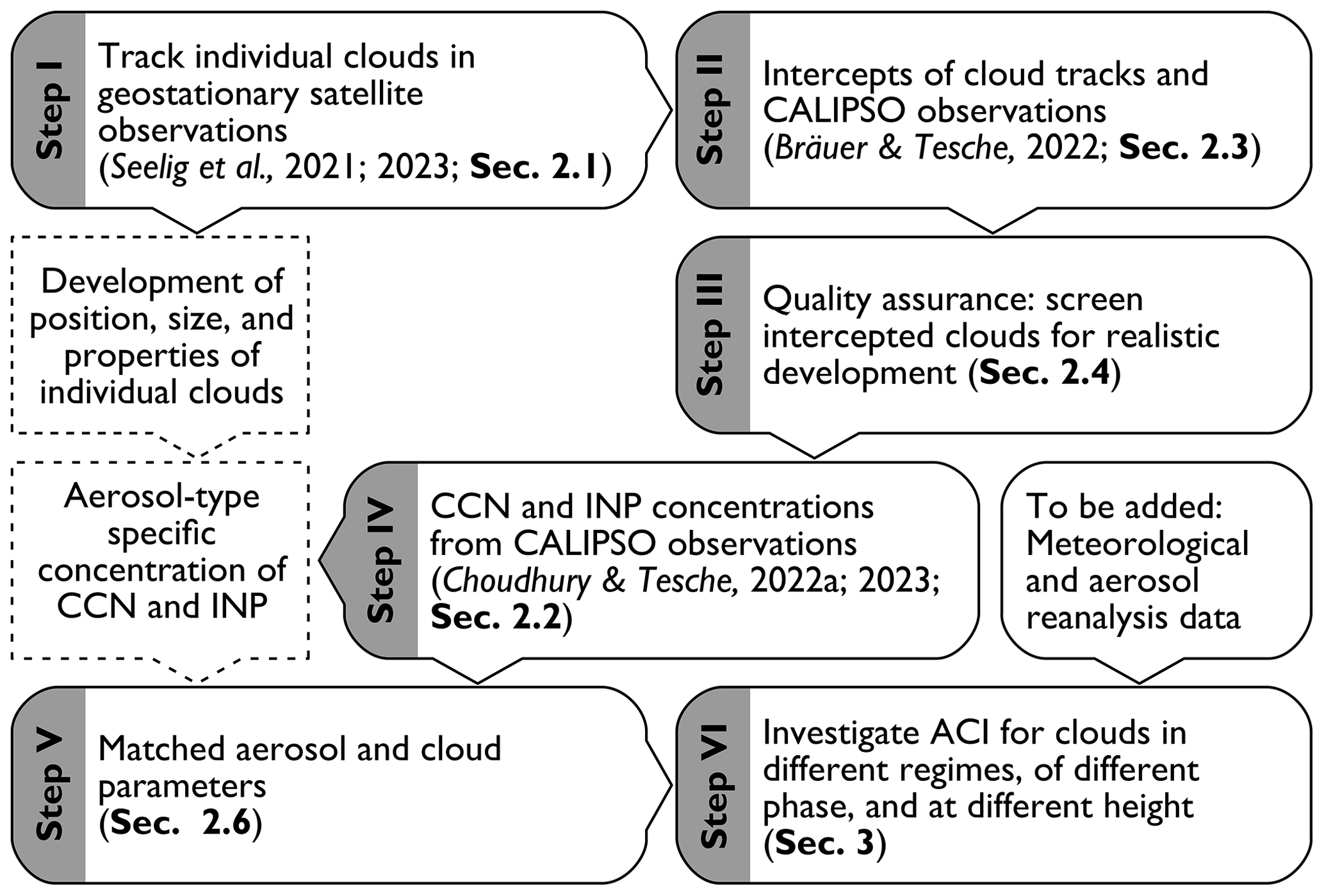
Figure 1 Flow chart of the different steps in the data analysis (solid boxes), with references to the corresponding literature and sections in this paper, and the inferred data products (dashed boxes).

2.1 Cloud tracking in geostationary satellite observations

The cloud-tracking toolbox of Seelig et al. (2021, 2023) is used to track individual clouds in time-resolved observations with geostationary sensors. The algorithm identifies objects in 2 consecutive time steps and uses particle image velocimetry (Adrian and Westerweel, 2010) to create a velocity field between them in multiple overlapping windows of different sizes. This process determines the displacement that best matches objects in a pair of consecutive binary 2D images by means of cross-correlation. Matches between the objects from one time step to the next are created by considering the distance of the centroids of the identified objects and their overlapping area. The best match within set thresholds is kept if the difference in area does not exceed a factor of 4. This areal threshold ensures realistic growth (decay) rates for non-merging (non-splitting) clouds and is based on our observations of small clouds – particularly the growth of one-pixel and two-pixel clouds. In the case of a splitting event (one object is matched to multiple objects), one match is chosen arbitrarily. In the case of a merging event (multiple objects are matched to one object), the best match is kept. In the case of a tie, again, one match is chosen arbitrarily. This process is repeated for all consecutive time steps to form a trajectory of a tracked object.

This method has so far been applied to the binary cloud mask inferred from observations of MSG-SEVIRI (Seelig et al., 2021) and the Advanced Baseline Imager (ABI; Schmit et al., 2017) aboard NASA's Geostationary Operational Environmental Satellites – R Series (GOES-R ABI) (Seelig et al., 2023). Cloud physical properties (CPP) can be derived from those observations only during the daytime, as visible reflectances are needed for the retrieval. The CPP generally include T_top, cloud top height (h_top), cloud top pressure (p_top), COT, r_eff, and L. N_d is derived using COT and r_eff (Grosvenor et al., 2018; Quaas et al., 2020). This work uses CPP derived from MSG-SEVIRI observations and provided in the CLAAS-2 (Benas et al., 2017) data set with a temporal resolution of 15 min. These CPP are matched to the trajectories of tracked clouds to obtain mean and median values per time step and for the lifetime of individual clouds.

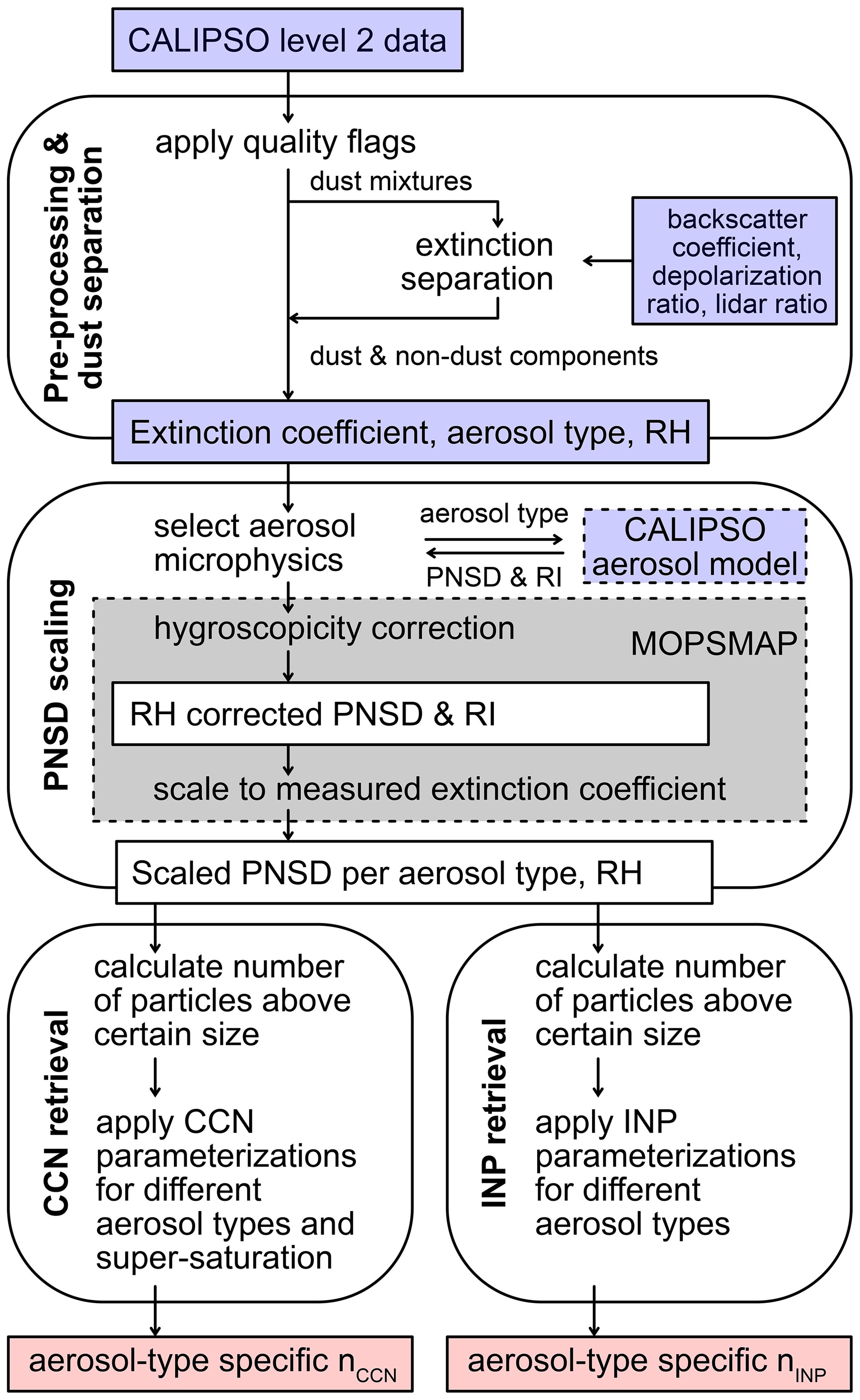
Figure 2 Flow chart of the OMCAM retrieval for inferring n_CCN and n_INP from spaceborne CALIPSO lidar observations. Input from CALIPSO measurements and the CALIPSO aerosol model is marked by blue boxes. The grey area covers the hygroscopicity correction and particle number size distribution (PNSD) scaling with the help of MOPSMAP. White boxes mark intermediate products. The final n_CCN and n_INP for different aerosol types are given in the pink boxes. RH and RI relate to relative humidity and refractive index respectively. Figure revised from Choudhury and Tesche (2022a).

For a first application of the C×C approach, we want to focus on low-level liquid clouds and mid-level mixed-phase clouds as observed by MSG-SEVIRI over Europe, the Mediterranean, and northern Africa. As outlined in Seelig et al. (2021, 2023), the data set of all tracked clouds is filtered to obtain sub-samples that correspond to the targeted cloud types. Firstly, a cloud has to show a cloud top height that relates to the targeted cloud type. Secondly, a cloud has to form and dissolve in clear air to provide assurance that well-defined development can be observed. Finally, a cloud has to occur entirely during the daytime so that CPP data are available throughout its lifetime.

2.2 Cloud-relevant aerosol concentrations from spaceborne lidar observations

Ground-based lidar measurements provide great potential for inferring height-resolved CCN and INP concentrations (Mamouri and Ansmann, 2016; Marinou et al., 2019). However, adaptation of the ground-based approach to spaceborne lidar observations is not straightforward, as the required extinction-to-number-concentration conversion factors show strong regional variation (Ansmann et al., 2019). The Optical Modelling of CALIPSO Microphysics (OMCAM; Choudhury and Tesche, 2022a) algorithm provides an alternative approach for inferring CCN concentrations from spaceborne Cloud-Aerosol Lidar and Infrared Pathfinder Satellite Observations (CALIPSO; Winker et al., 2009) lidar observations that is consistent within the wider CALIPSO retrieval. Figure 2 presents a flow chart of the OMCAM algorithm. In short, quality-assured CALIPSO Level 2 aerosol profiles are used to obtain aerosol-type specific extinction coefficients (upper panel in Fig. 2) that constrain light-scattering calculations (Gasteiger and Wiegner, 2018) based on the normalized size distribution and complex refractive indices (middle panel in Fig. 2) for different aerosol types in the CALIPSO aerosol model (Omar et al., 2009). The scaled size distribution relating to the modelled extinction coefficient that best reproduced the measurement is then integrated from a lower size limit at which the different aerosol types are likely to be relevant for cloud properties to obtain the number concentration of reservoir particles (lower panels in Fig. 2). The latter are then used as input to commonly used parametrizations (DeMott et al., 2010, 2015; Steinke et al., 2015; Ullrich et al., 2017) to infer CCN and INP number concentrations, n_CCN and n_INP respectively. For more details on the OMCAM retrieval and its uncertainties, readers are referred to Choudhury and Tesche (2022a).

Thorough validation of OMCAM-derived n_CCN generally finds values that are within a factor of 1.5 to 2.0 of independent airborne and ground-based in situ observations (Aravindhavel et al., 2023; Choudhury et al., 2022; Choudhury and Tesche, 2022b), which is far less than their natural variability. OMCAM-derived data have been used to compile a global height-resolved n_CCN climatology from 15 years of CALIPSO observations (Choudhury and Tesche, 2023a) that can be used complementary to model-derived n_CCN (Block et al., 2023) as a benchmark for cloud-resolved climate modelling.

For this work, OMCAM was expanded analogous to Mamouri and Ansmann (2016) and Marinou et al. (2019) to estimate the concentration of INP reservoir particles which are subsequently used as input to INP parametrizations to obtain n_INP (lower-right panel in Fig. 2). This capability allows us to extend the scope of the C×C approach towards studying aerosol effects on ice-containing clouds. In contrast to n_CCN, independent in situ measurements of n_INP are sparse. This is why the validation of OMCAM-derived values is still a matter of ongoing research. Nevertheless, initial findings based on comparison to airborne in situ measurements indicate that CALIPSO-derived n_INP have a quality comparable to those inferred from ground-based lidar measurements (Marinou et al., 2019; Choudhury et al., 2022).

2.3 Matching cloud trajectories with aerosol observations

The intercept points between individual cloud trajectories and the CALIPSO ground track are obtained with the TrackMatcher tool (Bräuer and Tesche, 2022; https://github.com/LIM-AeroCloud/TrackMatcher.jl.git, last access: 18 March 2024). The purpose of TrackMatcher is the identification of intercept points between two lines on a latitude–longitude grid and the collocation of the respective data fields along those tracks. In the context of the C×C approach, this enables us to match cloud properties along a cloud trajectory from geostationary satellite observations (Sect. 2.1) to the surrounding cloud-relevant aerosol concentrations from polar-orbiting lidar observations (Sect. 2.2). The algorithm allows us to find intersections in any pair of tracks that provide information on time (t), latitude (φ), longitude (λ), and height (h). The main steps of the algorithm are to (i) load track data related to two platforms, (ii) interpolate the individual tracks using a piecewise cubic Hermite interpolating polynomial, (iii) find intersections by minimizing the norm between the different track point coordinate pairs, and (iv) extract auxiliary information at or around the intercept point as set by the operator. For applying the C×C approach, the auxiliary formation extracted from the CALIPSO Level 2 aerosol profile product consists of height profiles of the OMCAM input parameters, i.e. backscatter and extinction coefficients, particle linear depolarization ratio, vertical feature mask, and cloud–aerosol discrimination (CAD) score. In addition, the accepted time difference between the two tracks can be chosen to best suit the application. In this study, we did not limit the time difference for finding matches between a cloud track and the CALIPSO satellite, but most cases fell within a range between 0 and ± 90 min. This time difference is well below the timescale for which major changes in an aerosol field could be expected (Anderson et al., 2003; Kovacs, 2006).

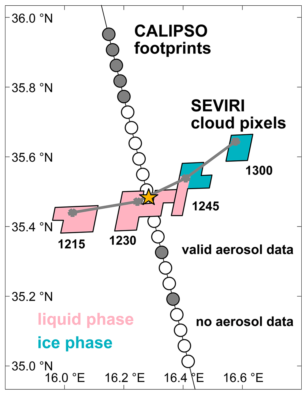
Figure 3 Example for matching a SEVIRI cloud trajectory from 12:15 to 13:00 UTC on 20 March 2014 (grey line connecting the centroids of each time step) with the 5 km averaged footprints along the CALIPSO ground track for an overpass at 12:15 on 20 March 2014. Filled CALIPSO footprints mark profiles with valid aerosol data, while empty circles refer to profiles without aerosol information. The yellow star marks the intercept point. Pink and blue areas refer to SEVIRI pixels for which cloud water is identified as liquid and ice respectively.

An example for matching a cloud trajectory with a CALIPSO measurement is presented in Fig. 3. CALIPSO Level 2 data are available in 5 km intervals along the ground track, while the example trajectory consists of four time steps. When a match is made, CALIPSO profiles are filtered for quality-assured data at the height levels of the paired cloud following the criteria summarized in Table 1 of Tackett et al. (2018). Aerosol data might be absent or dismissed in cases of low aerosol load (low signal-to-noise ratio), retrievals with low confidence scores, or cloud presence. In Fig. 3, the cloud changes from purely liquid (time steps 1 and 2) to mixed-phase (time step 3) to purely ice (time step 4). Aerosol information is available in the vicinity of the matching point and can be used to infer mean CCN or INP concentrations surrounding the tracked cloud. Further details on this procedure are provided below.

2.4 Quality-assured development of matched clouds

Our cloud tracking (Sect. 2.1) is generally performed on a binary cloud mask in which pixels are differentiated as either cloud or cloud-free. In passive observations, cloudy pixels do not unambiguously refer to a specific cloud type (Rossow and Schiffer, 1999). Instead, the column information observed at the top of the atmosphere might actually be the product of contributions of very different clouds, such as low-level water clouds and high-level ice clouds. While these contributions will not be discernible in a cloud mask, they will propagate into the inferred cloud physical properties. Clouds that are found to intercept a CALIPSO overpass (Sect. 2.3) therefore have to undergo quality assurance before they can be considered for further analysis.

This quality screening is performed in two steps. Clouds are initially sorted according to their phase and subsequently investigated for realistic development of their physical properties. The phase categorization sorts clouds as

1. liquid-water if (i) the phase of all pixels is liquid or (ii) the median cloud top temperature is warmer than −5 °C;

2. mixed-phase if there are both liquid and ice pixels in the temperature range from −5 to −38 °C;

3. ice (heterogeneously frozen) if there are only ice pixels in the temperature range from −5 to −38 °C;

4. ice (homogeneously frozen) if the median cloud top temperature of all pixels is lower than −38 °C.

The objective of our C×C approach is to investigate liquid-water clouds for their response to changes in CCN concentrations and in mixed-phase and heterogeneously frozen ice clouds for their response to changes in INP concentrations. To obtain meaningful results, however, we need to exclude those clouds that appear to evolve non-physically, i.e. that show a large variation in their properties from time step to time step or throughout their lifetime. We have therefore identified four objective criteria for assessing realistic cloud development based on cloud top temperature, area, and phase. A cloud is flagged if it shows

1. unrealistic development of T_top from start to end (the norm of the difference between median T_top at cloud beginning and end exceeds 30 K);

2. unrealistic development of T_top between time steps (the norm of the change in median T_top from time step to time step exceeds 15 K);

3. unrealistic spread of T_top within individual time steps (the spread in T_top (maximum T_top to minimum T_top per time step) exceeds 35 K for more than 50 % of all time steps);

4. unrealistic development of cloud size (the change in cloud size from time step to time step for clouds that consist of more than four pixels exceeds 100 %; i.e. cloud size should neither double nor half).

These criteria apply to the entire trajectory. A cloud is kept for by-eye inspection if one of criteria 1 to 4 is met. It is dismissed (considered as unrealistic) if multiple criteria are met. The latter also applies if criterion 2 or 4 is met multiple times. While this rigorous screening of tracked clouds implies a high level of data reduction, it ensures that only cases in which the observations show a cloud that develops in a physically meaningful way along its trajectory (i.e. that are not affected by any of the limitations of passive remote sensing) will be considered in the subsequent investigation of aerosol–cloud interactions. In other words, we can only obtain robust findings from the bottom-up database if the highest level of scrutiny is applied in the identification of trustworthy aerosol–cloud cases.

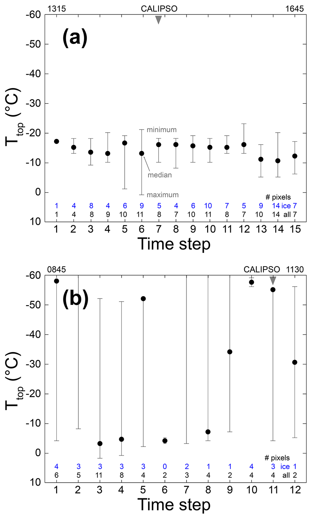
Figure 4 Realistic (a) and unrealistic (b) development of T_top, cloud area, and cloud phase found on 14 August 2014 and 24 March 2014 respectively. T_top per time step refers to the median over all cloud pixels (black dot), while the range marks the temperatures of the warmest (lower whisker) and coldest (upper whisker) pixel respectively. Numbers at the bottom refer to the size of the cloud in pixels (black) and the number of pixels identified as ice (blue). The start and end times (in UTC) of the trajectories and the time of the CALIPSO observation (grey triangle) are given at the top of the plot.

Figure 4 presents the development of two tracked clouds to illustrate the quality assurance methodology. The example cloud on 14 August 2014 shows a development that we consider as realistic. The cloud was tracked from its formation at 13:15 UTC until it dissolved at 16:45 UTC. Median, minimum, and maximum T_top values all vary within a reasonable range throughout all 15 min time steps. The cloud is partly or fully glaciated at temperatures where this is not unlikely. The change in cloud size is indicative of plausible growth and decay rather than merging and splitting. Overall, this case represents a heterogeneously frozen ice cloud that can be used in studies of the effect of surrounding INP concentrations on cloud properties and development. In contrast, the example cloud on 24 March 2014 raises some of the flags listed above. Over the length of its existence from 08:45 to 11:30 UTC, median T_top shows multiple time-step-by-time-step changes of more than 15 K (criterion 3). This indicates the coinciding presence of low and high clouds within the cloud area or even on a pixel basis, and it would already lead us to dismiss that cloud as unrealistic. The spread in T_top per time step exceeds 35 K for 10 out of 12 time steps (criterion 4) provides another indication that clouds at different height levels contribute to the column signal detected in the passive observation. Finally, the areal growth from time step 2 to time step 3 exceeds a doubling (criterion 2), and the norm of the difference in T_top at the first and last time steps is very close to 30 K (criterion 1).

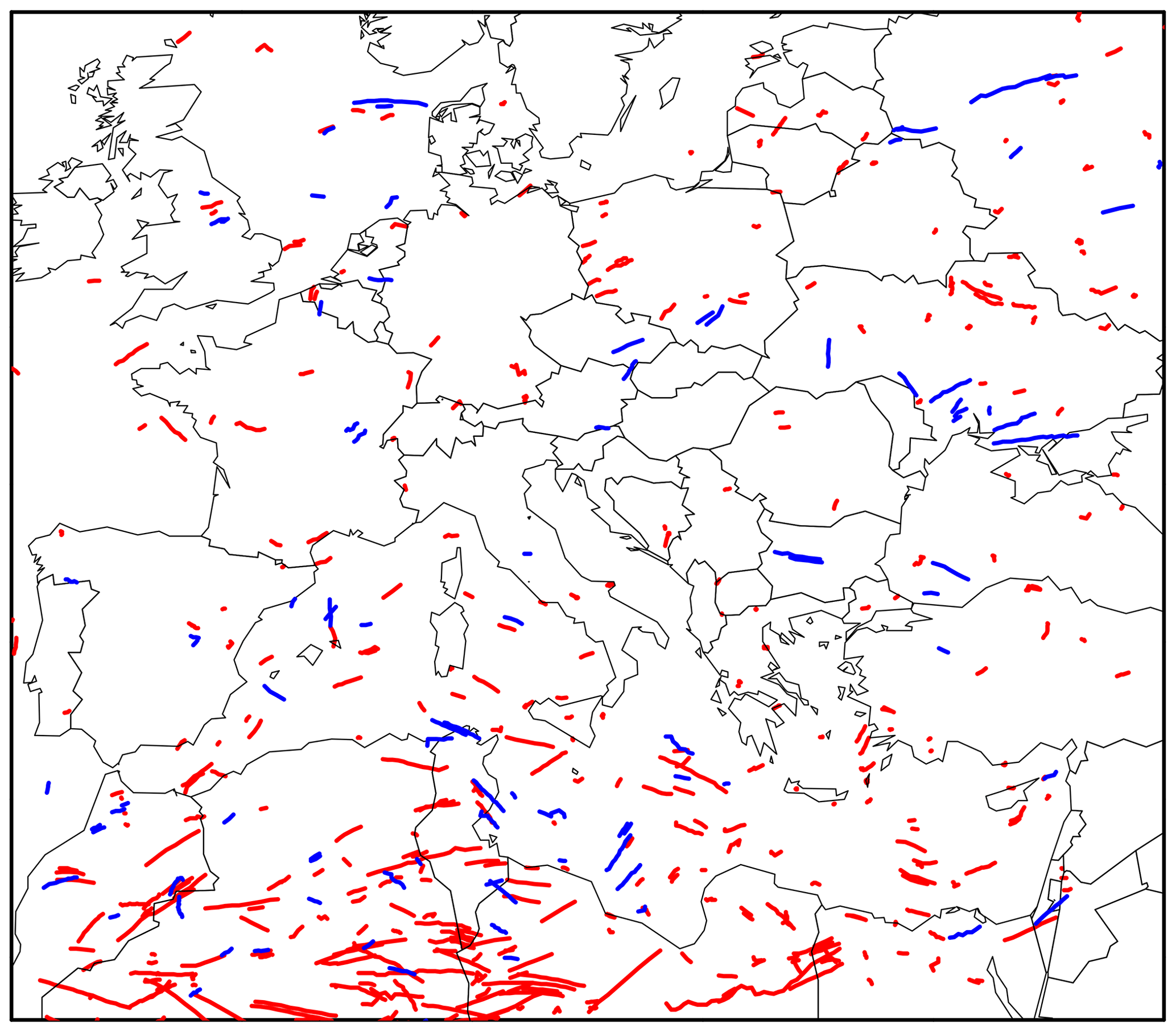
Figure 5 Overview of the study region with trajectories of liquid-only (red, N=399) and ice-containing (blue, N=95) clouds that could be matched to surrounding n_CCN and n_INP respectively.

The consideration for realistic cloud development puts another constraint on the selection of cases that can actually be used in the formation of our bottom-up database. Overall, the initial matching of trajectories to CALIPSO overpasses, followed by the demand for valid aerosol observations at cloud level and the subsequent requirement for realistic cloud development, reduces the database from an order of 1 million tracked clouds to an order of a few hundred cases for consideration in our C×C approach. We have opted for the exceptionally high level of scrutiny despite the resulting poor data yield to provide assurance that findings later inferred from the bottom-up database are physically meaningful. In future, the length of the available time series of around 15 years, the possibility to extend the CCN and INP retrievals to newer spaceborne lidar missions, the option for expanding the study area, and the application to further geostationary sensors provide ample opportunities for extending the number of cases without compromising their quality.

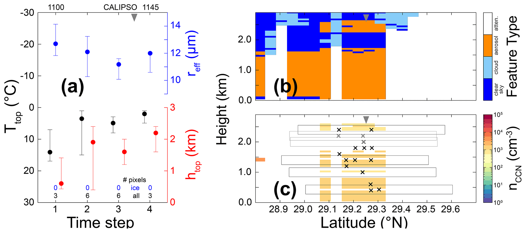
Figure 6 Example of (a) the development of T_top (black), h_top (red), and r_eff (blue) for a liquid-only cloud observed by MSG-SEVIRI between 11:00 and 11:45 UTC on 18 March 2014 and the surrounding aerosol field from CALIPSO lidar observations in terms of (b) the feature type and (c) n_CCN for an overpass at 11:37 UTC. The grey triangles mark the intercept between the cloud trajectory and the CALIPSO ground track. The example boxes in (c) illustrate the along-track distance and height range centred around the location and h_top (crosses) of individual pixels in panel (a) used for matching aerosol and cloud data. Successful matches (i.e. valid CCN data available within a set distance to a pixel of a tracked cloud) are given in black, while matches without valid CCN data are marked grey. White in panel (b) marks regions where the lidar signal has already been fully attenuated from clouds above. Note that not all detected aerosol features (orange in panel b) provide CCN information as the result of applying quality flags in the CCN retrieval (see Fig. 2).

2.5 Study region

For testing the new C×C approach, we have selected a region that covers Europe and northern Africa. Figure 5 shows that our study region extends from the Atlantic coast to eastern Ukraine and from southern Sweden to the southern tip of Tunisia and the Sinai Peninsula. All four cloud categories listed in Sect. 2.4 are found in the study region. In addition, the region covers the pathways of mineral dust transport to Europe. This is of particular interest to our work, as mineral dust particles are very efficient INPs and are most likely to cause detectable changes in cloud phase.

2.6 Deriving matched aerosol and cloud parameters

The data obtained from matching the information related to tracked cloud properties and cloud-relevant aerosol properties are presented based on the case study of 18 March 2014 shown in Fig. 6. A liquid-water cloud could be tracked for four time steps between 11:00 and 11:45 UTC. Its first time step shows a median T_top of about 14 °C which corresponds to a h_top of about 500 m. The median r_eff for this initial time step is 12.5 µm. Over the next three time steps, T_top decreases to 2 °C as h_top increases to 2.2 km. At the same time, r_eff decreases slightly to 12 µm. Throughout its lifetime, the cloud consisted of 18 pixels of which none revealed the presence of ice. The CALIPSO lidar overpass matched with this trajectory occurred at 11:37 UTC between the third and fourth time step of cloud lifetime. Around the overpass, CALIPSO measurements reveal the presence of aerosols and clouds with upper-level clouds attenuating the lidar signal before it can reach the surface (Fig. 6b). The OMCAM retrieval gives an estimated n_CCN of around 2000 cm⁻³ between the surface and 2.5 km height – well within the height range of the observed cloud.

Pixel-wise, cloud properties are matched to the aerosol field within an along-track distance of thirteen 5 km CALIPSO intervals and five 60 m height bins around the pixel's h_top. Valid data in CCN concentration within such a box is averaged to obtain a median n_CCN that can be related to the cloud properties. In the example in Fig. 6, 14 cloud pixels show values of h_top that allow us to assign a median n_CCN to their cloud properties, while 4 pixels reveal values of h_top that fell within a height range for which no CCN information could be retrieved. Consequently, the case of 18 March 2014 contributes 14 pairs of matched aerosol–cloud information to the statistical analysis presented below.

To summarize, the C×C approach allows us to decompose clouds at three stages:

1. The pixel stage considers individual cloud pixels and the CALIPSO aerosol with 13 profiles by 5 height bins around the pixel's h_top. This is referred to as pixel-wise information in this paper.

2. The time step stage considers cloud and aerosol mean and median values for individual time steps of a considered cloud. This information is not used in this paper.

3. The trajectory stage considers cloud and aerosol mean and median values for the entirety of a cloud trajectory, i.e. all time steps. This is referred to as whole-trajectory information in this paper.

3 Results

3.1 General overview

For a first application of the C×C approach, we want to focus on (i) liquid clouds which have been extensively studied with other methods and (ii) ice-containing clouds for which our new approach will enable us to assess the impact of INP concentrations on cloud phase and development. The tracking of clouds in CLAAS-2 data (Sect. 2.1) within the region of interest (Fig. 5) for 2014 gives a total of 8 924 639 trajectories of clouds with well-defined start and end points, i.e. forming and dissolving in clear air. The matching procedure outlined in Sect. 2.3 implies rigorous screening of that data set to trajectories that coincide with a CALIPSO observation during both day and night. This constraint reduces the number of data to 4393 tracked and matched clouds that could potentially be used for further investigation. Out of those, 964 daytime trajectories of liquid clouds are found to be vertically co-located with CCN layers (Sect. 2.2). Further quality assurance regarding realistic cloud development (Sect. 2.4) finally gives 399 trajectories for further analysis. In the case of ice-containing clouds, 844 daytime trajectories could be matched to vertically co-located INP layers of which 95 clouds remained after quality assurance (Sect. 2.4). Following the phase categorization in Sect. 2.4, the ice-containing clouds can be further separated into 42 clouds that are homogeneously frozen, 8 clouds that are heterogeneously frozen, and 45 mixed-phase clouds. The data set of liquid clouds also contains 37 trajectories of supercooled clouds for which neither the median T_top per time step exceeds 0 °C nor cloud ice is detected. These supercooled liquid clouds provide a reference in studying the impact of n_INP on the ice-containing clouds.

Figure 5 gives an overview of the cloud trajectories that could be matched to aerosol information from CALIPSO measurements over Europe and northern Africa for the year 2014. We will start with a description of the matched data sets before presenting the first results of applying the C×C approach for studying liquid-water and ice-containing clouds.

3.2 The matched aerosol–cloud data sets

The data set of matched cases for the year 2014 within the study region in Fig. 5 consists of 399 trajectories of liquid clouds and 95 trajectories of ice-containing clouds. Both cloud types are rather small and short-lived. They span lifetimes from 3 to 47 (3 to 20 for ice-containing clouds) time steps of 15 min with a median of 4 time steps. The histogram of trajectory length in Fig. 7 shows that the majority of clouds exist for less than 2 h. The size of the liquid clouds per time step ranges from 1 to 341 pixels with a median of 5 pixels (not shown). Clouds consisting of 10 pixels or fewer make up 70 % of the data set. The ice-containing clouds considered here are smaller than the liquid clouds with sizes ranging from 1 to 53 pixels, a median of 4 pixels, and 90 % of clouds consisting of 15 pixels or fewer (not shown).

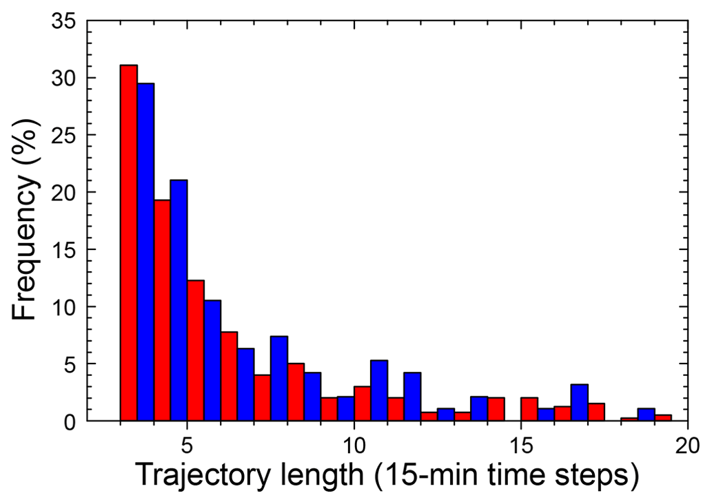
Figure 7 Frequency of occurrence of trajectories of different lengths in 15 min time steps for trajectories of 399 tracked liquid-only (red) and 95 ice-containing (blue) clouds that could be matched to CALIPSO overpasses with valid aerosol data.

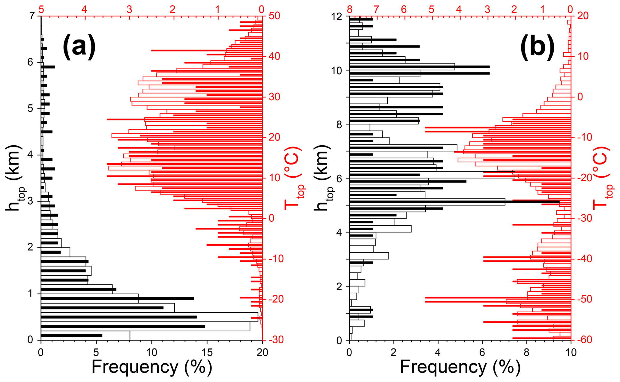
Figure 8 Frequency of occurrence of h_top (black) and T_top (red) of liquid (a) and ice-containing (b) clouds that could be matched to CALIPSO overpasses with valid aerosol data. Open bars refer to pixel-wise information (35 799 for liquid-only, 4016 for ice-containing), and solid bars mark whole-trajectory medians (399 for liquid-only, 95 for ice-containing). Note that data relating to the left and right scales respectively are independent of each other.

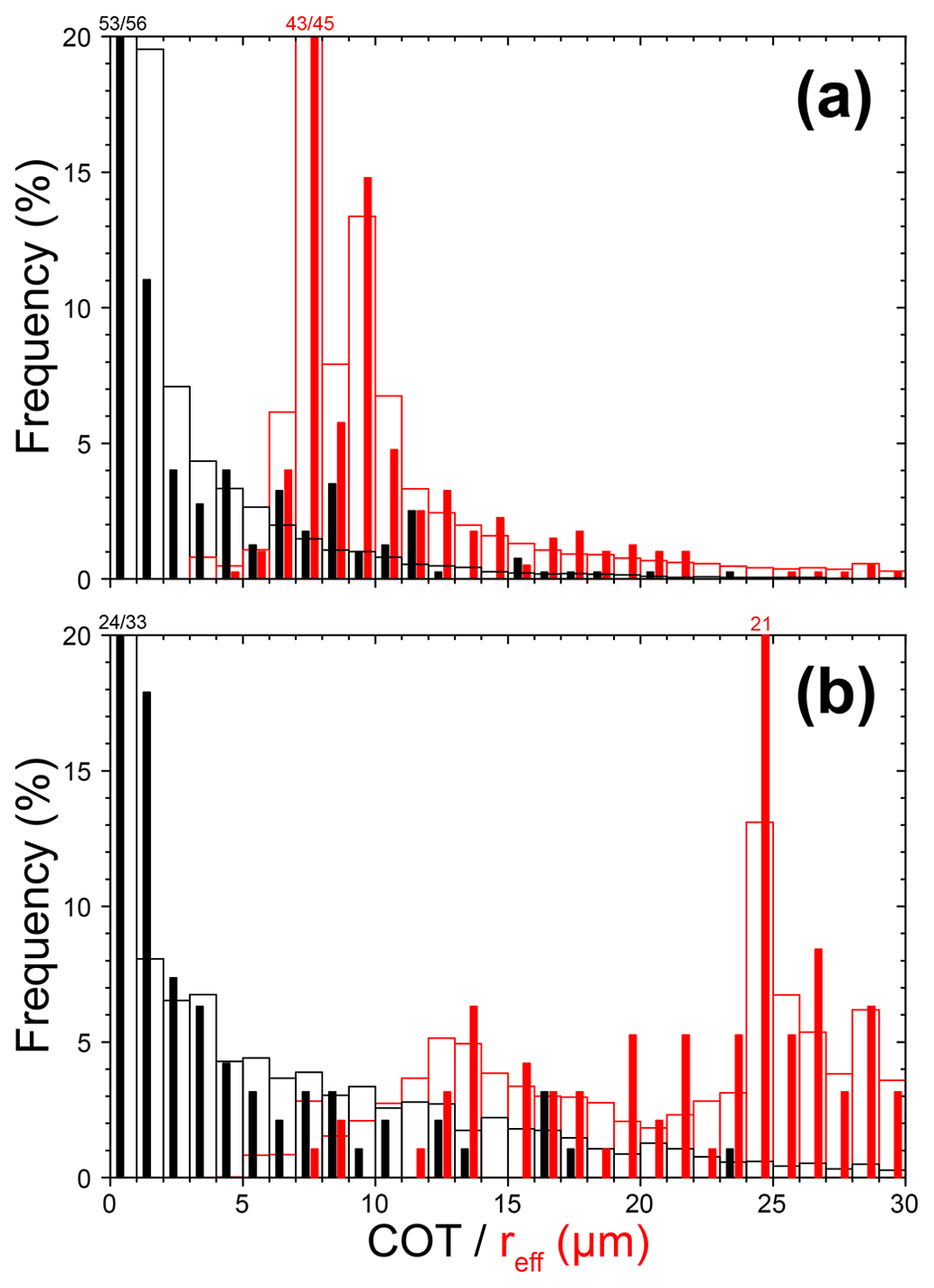
Figure 9 Frequency of occurrence of COT (black) and r_eff (red) for (a) liquid-only and (b) ice-containing clouds that could be matched to CALIPSO overpasses with valid aerosol data. Note that the number of pixels with valid cloud information is reduced compared to Fig. 8. Open bars refer to pixel-wise information (24 089 out of 35 799 available pixels for liquid-only clouds and 3769 out of 4016 available pixels for ice-containing clouds), and solid bars mark whole-trajectory medians (399 for liquid-only, 95 for ice-containing). Numbers at the top of the plots refer to the pixel-wise and whole-trajectory values related to the intervals for which the frequency of occurrence exceeds the scale.

Figure 8 gives an overview of the distribution of h_top and T_top of the liquid and ice-containing clouds that could be matched with information of the surrounding aerosol field. Most liquid clouds persist below 1.0 km. The median h_top is 0.6 km, while the occurrence of few pixels with large h_top increases the mean to 0.9 ± 1.1 km. The majority of cloud pixels (95 %) show positive values of T_top with a mean of 21.0 ± 12.4 °C and a median of 20.9 °C. These comparably high temperatures are related to the fact that a large number of tracked clouds are located over northern Africa (see Fig. 5). Cloud pixels with negative T_top in the liquid data set refer to supercooled clouds, which can be used as a reference in the investigation of the effect of n_INP on ice-containing clouds. When data are aggregated to represent the median values of entire trajectories, h_top slightly increases to 1.3 ± 1.5 km with a median of 0.8 km, while T_top decreases correspondingly to 17.4 ± 15.0  °C with a median of 16.9 °C. The overview of the ice-containing clouds in Fig. 8b shows that those clouds generally occur at larger heights and lower temperature than the liquid clouds. One group of ice-containing clouds occurs at $T_{\text{top}}<-\mathrm{38}$ °C and h_top>8 km, which is in line with the regime of homogeneous freezing. The other group with $T_{\text{top}}>-\mathrm{38}$ °C covers the regime of heterogeneous freezing (i.e. INPs are needed to form cloud ice; Kanji et al., 2017) and represents the temperature range at which supercooled, mixed-phase, and ice clouds can be observed. We expect that the latter clouds would be most susceptible to changes in aerosol concentrations. They make up 2673 pixels (53 clouds) with h_top ranging from 0.4 to 9.7 km (0.8 to 9.2 km) and a median of 5.8 km (5.7 km). When considering all ice-containing clouds, the pixel-wise (whole-trajectory) mean values are $h_{\text{top}}=\mathrm{6.8}\pm \mathrm{2.4}$ km (7.5±2.5 km) and $T_{\text{top}}=-\mathrm{23.6}\pm \mathrm{18.5}$ °C ($-\mathrm{30.0}\pm \mathrm{18.8}$ °C), with median value of 6.6 km (7.2 km) and −17.2 °C (−25.2 °C).

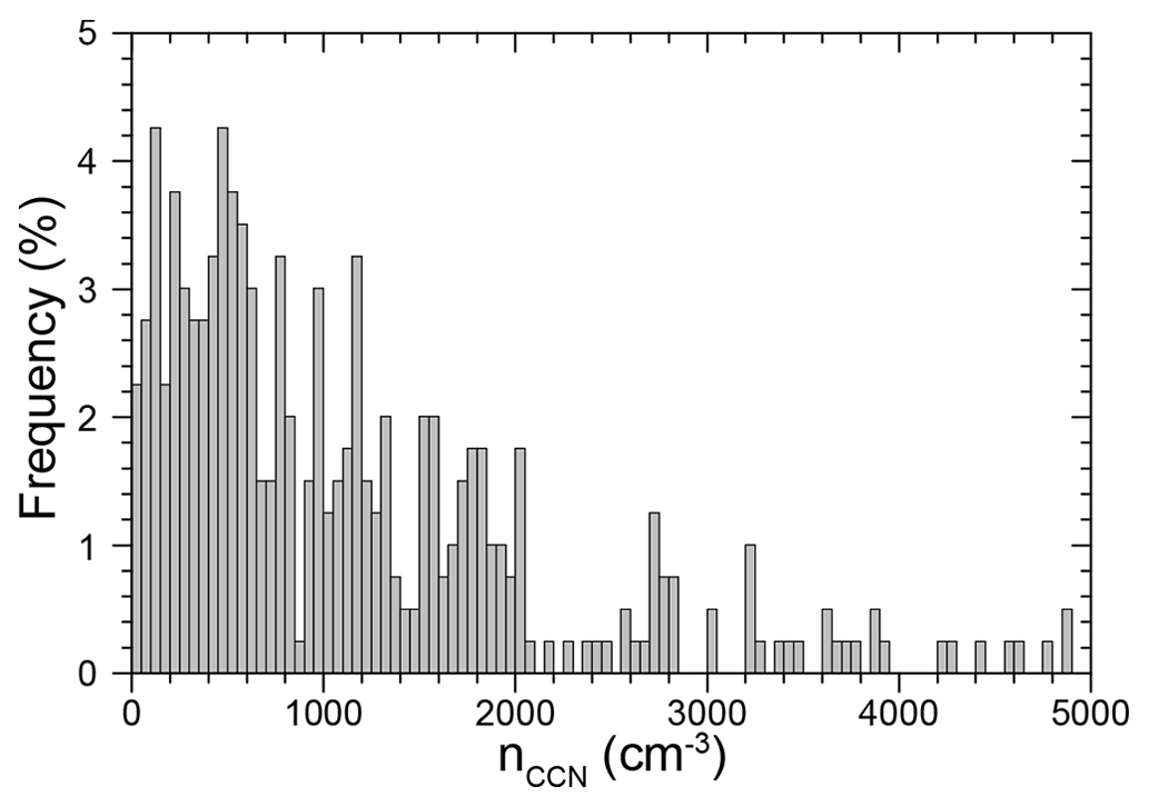
Figure 10 Frequency of occurrence of median n_CCN for 399 CALIPSO overpasses that could be matched to tracked liquid-only clouds.

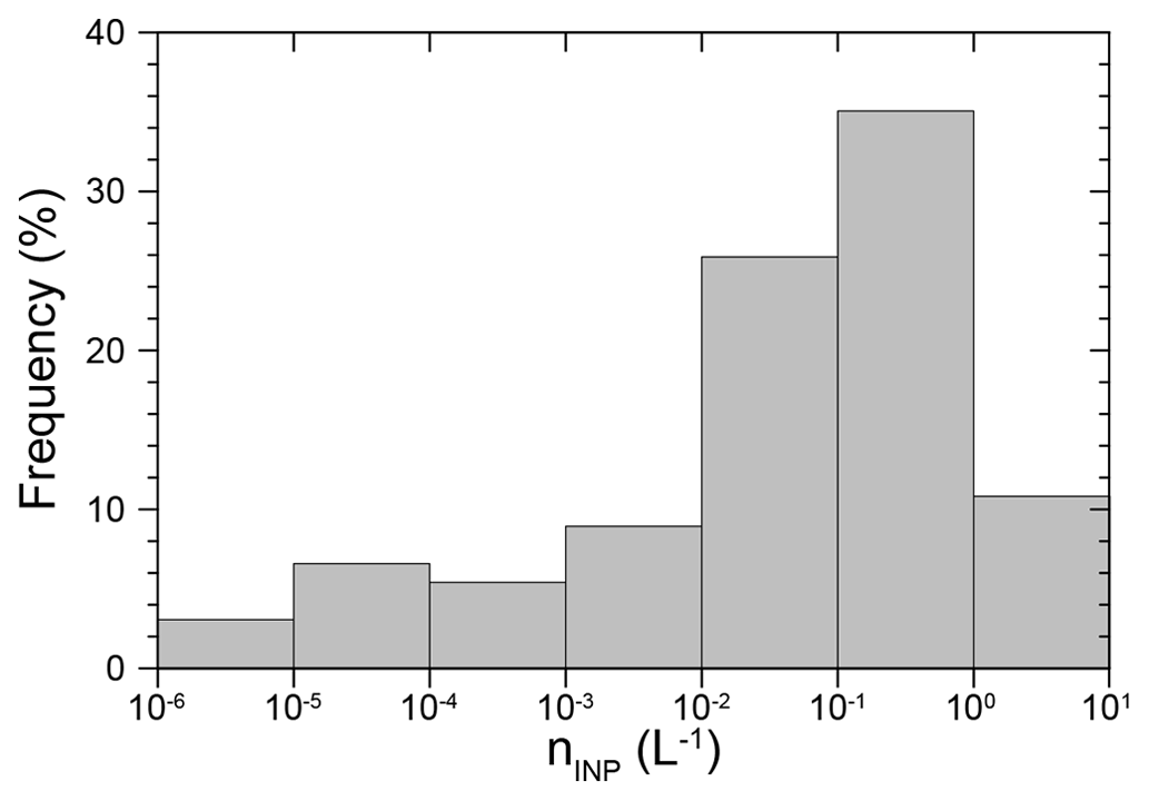
Figure 11 Frequency of occurrence of median n_INP for 95 CALIPSO overpasses that could be matched to tracked ice-containing clouds.

The pixel-wise and whole-trajectory histograms of COT and r_eff for both liquid and ice-containing clouds are presented in Fig. 9. Because retrievals of cloud microphysical properties require data at visible wavelengths, this information is available only during the daytime. Hence, and as a result of measurement restrictions such as weak signal-to-noise ratio, not all tracked pixels provide meaningful data. The majority of liquid clouds are optically thin with medians of 0.92 and 0.74 and means of 2.38 ± 5.23 and 2.47 ± 3.83 for the pixel- and trajectory-based analysis respectively. About 75 % of all cases are below the mean value. For ice-containing clouds, these values increase to pixel- and trajectory based medians of 4.88 and 1.85 and means of 8.26 ± 10.77 and 3.94 ± 4.86 respectively. An even larger difference is revealed in the size of the cloud particles. For liquid clouds, the median r_eff is 7.8 µm for both the pixel- and trajectory-based analysis with means of 10.1 ± 5.0 µm and 9.8 ± 4.0 µm respectively. Only 15 % of cases show median values larger than 12 µm, which indicates the likely presence of precipitation (Rosenfeld et al., 2012). The presence of ice in clouds increases the inferred values of r_eff to pixel- and trajectory-based means of 20.9 ± 7.5 µm and 22.0 ± 5.7 µm and medians of 23.2 and 24.4 µm respectively.

The histogram of n_CCN for the 399 matched liquid clouds in Fig. 10 shows that the C×C approach is capable of covering a wide range of CCN conditions. While values range from 17 to 25 721 cm⁻³ with a median of 872 cm⁻³, the majority of cases (about 90 %) are in a realistic range below 3000 cm⁻³. In the analysis of our data set, we will use n_CCN to discriminate between clean and polluted conditions. This is done in two steps. Firstly, the upper and lower 5 % of cases are dismissed from the data set, as they are likely to represent unrealistic values that result from propagating unreliable measurements through the analysis chain. For the present data set, this means that n_CCN<154 cm⁻³ and n_CCN>4409 cm⁻³, and the related cloud data are omitted from further analysis. While the exclusion of unrealistic values of n_CCN does not affect the data set presented here, it will become more crucial as the volume of the bottom-up data set increases. Secondly, the remaining 90% of cases is split into three ranges that represent clean (lower quantile), moderate (middle quantile), and polluted conditions (upper quantile). The resulting ranges contain about 4800 matched data points each and are 154 cm${}^{-\mathrm{3}}\le n_{\text{CCN}}<\mathrm{610}$ cm⁻³, 610 cm${}^{-\mathrm{3}}\le n_{\text{CCN}}<\mathrm{1210}$ cm⁻³, and 1210 cm${}^{-\mathrm{3}}\le n_{\text{CCN}}<\mathrm{4409}$ cm⁻³.

Figure 11 presents the histogram of n_INP related to the 95 ice-containing clouds. The majority of clouds (81 %) occur in aerosol fields that relate to values of n_INP between 10⁻³ and 10 L⁻¹ which are realistically found at atmospheric conditions (Kanji et al., 2017). About 3 % of inferred values fall outside the presented range of 7 orders of magnitude (2 % lower and 1 % higher). These values are likely the result of unreliable CALIPSO retrievals or originate from extrapolating the applied INP parametrizations to temperatures at which they are no longer applicable (Marinou et al., 2019). As in the case of n_CCN, unrealistic n_INP are excluded by dismissing the lowest and highest 5 % of values and related cloud data from further data analysis. As mentioned earlier, the detailed evaluation of the number concentration of reservoir particles and n_INP with independent in situ measurements analogous to Aravindhavel et al. (2023), Choudhury et al. (2022), and Choudhury and Tesche (2022b) is ongoing and will be the focus of a future publication.

3.3 CCN effects on liquid-water clouds

Now that we have obtained a data set of matched cloud and aerosol observations, we can start to investigate cloud properties for different ranges of n_CCN. Figure 12 shows that the mean n_CCN in the three quantiles mentioned before are 403 ± 110, 875 ± 189, and 2123 ± 733 cm⁻³. If the values of r_eff that have been matched to the aerosol observation are grouped according to those three n_CCN ranges, we can see a clear decrease in r_eff and an increase in N_d from clean to polluted aerosol conditions that is in line with the Twomey effect. While $r_{\text{eff}}=\mathrm{11.78}\pm \mathrm{6.6}$ µm (median of 9.0 µm) and $N_{\text{d}}=\mathrm{68}\pm \mathrm{166}$ cm⁻³ (median of 42 cm⁻³) for the lower third of n_CCN observations, values decrease to 9.99 ± 4.72 µm (median of 8.0 µm) and 75±100 cm⁻³ (median of 53 cm⁻³) for the middle third and even further to 9.34 ± 3.86 µm (median of 7.8 µm) and 95±199 cm⁻³ (median of 60 cm⁻³) for the upper third (see Fig. 12).

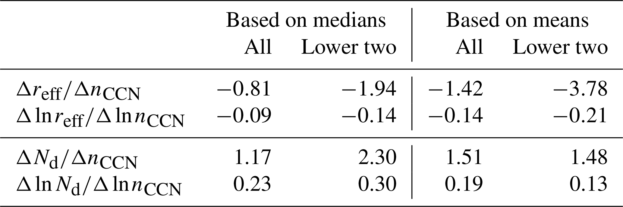
This allows a first quantification of the change in r_eff and N_d related to a change in n_CCN rather than aerosol proxies such as AOT or AI generally used in ACI studies based on satellite data (Bellouin et al., 2020; Quaas et al., 2020). An overview of the inferred sensitivities of r_eff and N_d to changes in n_CCN is provided in Table 1. We find a $\mathrm{\Delta }{r}_{\text{eff}}/\mathrm{\Delta }{n}_{\text{CCN}}$ in the range from −0.81 to −3.78 nm cm⁻³ depending on the considered quantiles and the use of median or mean values of the distributions in Fig. 12. In the same way, N_d is found to increase between 1.17 and 2.30 per increase of 100 cm⁻³ in n_CCN. The larger sensitivities found when derived over just the lower two quantiles (columns 4 and 6 in Table 1) corroborate that r_eff and N_d are most susceptible to changes in CCN concentration for low baseline values and that the effect becomes saturated with a further increase in n_CCN (Gryspeerdt et al., 2023).

For better comparison to studies based on passive CCN proxies, Table 1 also provides sensitivities for logarithmic changes. The analysis of the C×C data set gives values of $\mathrm{\Delta }\ln r_{\text{eff}}/\mathrm{\Delta }\ln n_{\text{CCN}}$ between −0.09 and −0.21 while $\mathrm{\Delta }\ln N_{\text{d}}/\mathrm{\Delta }\ln n_{\text{CCN}}$ is found to vary in the range from 0.13 to 0.30. The latter values are at the lower end of earlier findings of 0.3 to 0.8 based on column CCN proxies (Bellouin et al., 2020). There are likely two factors at play. Firstly, our study is the first one to derive sensitivities based on inferred CCN concentrations at cloud level. On the one hand, this ensures that we only consider cases in which the observed aerosols can actually interact with the observed clouds. On the other hand, cloud-layer n_CCN is likely to give a weaker aerosol signal than a column proxy, potentially reducing the deduced sensitivity. Secondly, the isolated clouds considered in the current data set might not be as sensitive to changes in aerosol concentration as e.g. widespread stratocumulus clouds (Bellouin et al., 2020; Gryspeerdt et al., 2017; Goren et al., 2019), or their lifetime might be too short to reveal the full impact of the aerosol perturbation (Glassmeier et al., 2021; Gryspeerdt et al., 2021). Future research based on a larger C×C data set will reveal if the lower sensitivity can be corroborated and if the regional variation of sensitivity of cloud parameters to changes in n_CCN can also be resolved with our new approach.

Table 1 Sensitivity of r_eff and N_d to changes in n_CCN. Values refer to the full range of n_CCN represented by the three quantiles in Fig. 12 (all) and the change from clean to moderately polluted conditions (lower two) and are based on median and mean values respectively. The unit for $\mathrm{\Delta }{r}_{\text{eff}}/\mathrm{\Delta }{n}_{\text{CCN}}$ is nm cm⁻³, while all other parameters have no units. However, $\mathrm{\Delta }{N}_{\text{d}}/\mathrm{\Delta }{n}_{\text{CCN}}$ is multiplied by 100, i.e. refers to a Δn_CCN of 100 cm⁻³.

Applying the same analysis to COT (mean and median of around 2 and 1 respectively), cloud lifetime (mean and median of 8 and 5 time steps respectively), and cloud top height (mean and median of 800 m and 600 m respectively) does not reveal any change in those parameters with changing aerosol concentration (not shown). For L, we find a decrease in the mean from 25 ± 47 g m⁻² for clean conditions to 16 ± 37 g m⁻² for polluted conditions. However, median values show comparable values around 5 g m⁻² for all three intervals of aerosol concentration in line with optically thin clouds. While these findings are not in line with the assumption that increased n_CCN increases cloud lifetime, albedo (COT), h_top, and L, we consider the results as still preliminary. The C×C approach will need to be applied to a longer time series and over a larger region to extend the data set for ACI studies from which more robust conclusions regarding the adjustments can be drawn. This will be the focus of follow-up work.

Furthermore, the use of CALIPSO observations allows us to allocate n_CCN to a specific aerosol type. In the data set presented here, mineral dust and polluted continental make up the most of the CCN population. Therefore, a specific aerosol-type investigation of the connection between n_CCN and r_eff will also be left for follow-up studies with a larger C×C data set.

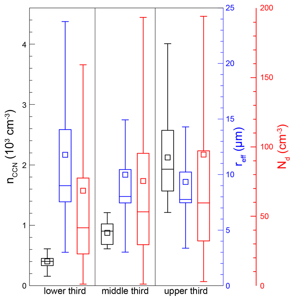
Figure 12 Boxplots of n_CCN (black), r_eff (blue), and N_d (red) for 16 230 matches of cloud pixels and aerosol information sorted into three quantiles. See text for details.

3.4 INP effects on ice-containing clouds

The capability of the C×C data set to provide information on n_INP and the development of the phase of a tracked cloud (Sect. 2.4) opens new avenues for also studying the effect of aerosols on ice-containing clouds. However, the related constraints for quality-assured cloud development and the lower abundance of successful INP retrievals from CALIPSO observations lead to a data set that is much smaller than the one for studying effects of changes in n_CCN on the properties of warm liquid-water clouds. Keeping this in mind, the current C×C data set for 1 year of data can only provide an outlook of its potential for spaceborne ACI studies.

The impact of n_INP on different cloud types in the regime of heterogeneous ice nucleation is illustrated in Fig. 13. We consider all clouds in Fig. 8 as supercooled if their whole-trajectory T_top and their T_top per time step never exceeded 0 °C and if all pixels were classified as liquid. These conditions are fulfilled by 42 clouds. Mixed-phase clouds have to show a combination of pixels that are classified as liquid and ice (see Fig. 3 for an example). This is the case for 45 clouds. Heterogeneously frozen clouds feature only pixels that are classified as ice and have to show values of T_top larger than −38 °C, which is the case for 8 clouds. Supercooled clouds show a mean T_top of $-\mathrm{11.7}\pm \mathrm{15.7}$ °C and a median of −6.2 °C. Mixed-phase clouds are colder with a mean T_top of $-\mathrm{14.0}\pm \mathrm{7.5}$ °C and a median of −11.2 °C), while heterogeneously frozen clouds show the lowest mean T_top of $-\mathrm{17.1}\pm \mathrm{3.7}$ °C and median of −16.9 °C. These clouds occur in an aerosol environment with mean n_INP values of 0.04±0.11, 0.23±0.31, and 2.64±1.79 L⁻¹ and medians of 0.02, 0.05, and 2.92 L⁻¹ respectively.

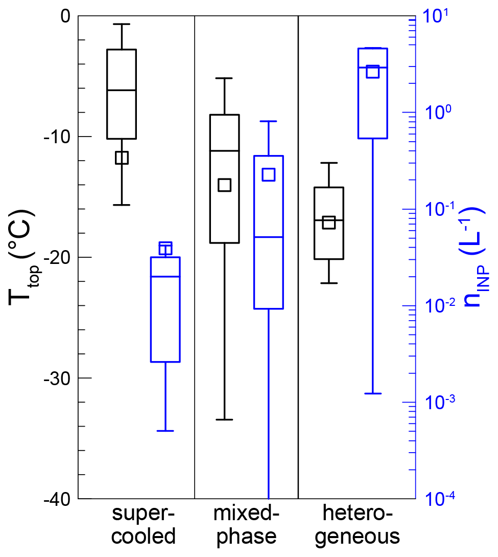
Figure 13 Boxplots of cloud-median T_top (black) and n_INP (blue) for supercooled liquid clouds (27 cases), mixed-phase clouds (45 cases), and heterogeneously frozen ice clouds (8 cases) as determined with the C×C approach. See text for details.

The parametrizations used to infer n_INP from the CALIPSO observations are strongly dependent on temperature. For mineral dust, they generally show an increase in n_INP by about 1 order of magnitude per 5 °C decrease (Marinou et al., 2019). The INP data set presented here consists primarily of CALIPSO observations in which the detected aerosols are classified as mineral dust. Hence, we would expect a similar relationship between the inferred T_top and n_INP of different cloud types if there was no change in the number of reservoir particles that could become INP-active, i.e. if there was no increase in aerosol concentration. Instead, we find that mean n_INP changes by about 1 order of magnitude already for a 3 °C decrease in mean T_top. This indicates that the increase in n_INP observed in the presence of mixed-phase clouds compared to supercooled clouds and of heterogeneously frozen clouds compared to mixed-phase clouds is not purely related to the decreasing T_top of the different cloud types but also to an increase in the concentration of aerosols that can act as INPs. In return, we can reason that the increased aerosol concentration facilitates earlier cloud glaciation as clouds surrounded by the largest abundance of INPs are fully glaciated, while those with medium and low n_INP are mixed-phase and liquid-phase respectively. This is in agreement with studies in which dust concentrations from aerosol reanalysis fields are used as a proxy for the presence of INPs (Seifert et al., 2010; Villanueva et al., 2020). Those studies address the issue by resolving the occurrence of ice-containing clouds within different ranges of T_top for different ranges of background aerosol concentrations, while our approach directly relates n_INP at cloud level to the occurrence of ice in the matched clouds. However, resolving a consistent picture through an entirely different data analysis concept increases our overall confidence in applying the C×C to both liquid-water and ice-containing clouds.

As in the case of liquid clouds, a larger data set is needed to obtain more robust constraints on the effect of aerosol concentrations on the properties of ice-containing clouds. This would facilitate e.g. assessing if variation in n_INP can also be found for supercooled, mixed-phase, and heterogeneously frozen clouds with comparable T_top, which would be a more direct indication of the effect of aerosol concentration on cloud phase.

4 Summary and outlook

We present a detailed description of a new approach for spaceborne ACI studies in which cloud development from geostationary satellite observations is matched with height-resolved CCN and INP concentrations from polar-orbiting satellite observations on a cloud-by-cloud (C×C) basis. The novel C×C approach has been applied to observations of MSG-SEVIRI and the CALIPSO lidar over Europe and northern Africa for the year 2014. Apart from the spatiotemporal matching of the observations, the analysis chain includes further screening to provide assurance that the resulting data set contains only (i) realistically developing clouds during the daytime for which macro- and microphysical properties can be inferred throughout their lifetime and (ii) scenarios in which cloud-relevant aerosols actually occur within the height range of the matched cloud.

Tracking objects in the CLAAS-2 cloud mask gives about 9 million clouds with a well-defined start and end, i.e. forming and dissolving in clear air, over the considered region throughout 1 year. Further data processing steps outlined in this paper reduce this number to 399 liquid clouds and 95 ice-containing clouds that can be matched to surrounding concentrations of CCN and INPs respectively at cloud level. Based on this initial data set, we demonstrate the potential of the C×C approach for spaceborne ACI studies with two examples: the sensitivity of N_d and r_eff to changes in n_CCN and the relation of the occurrence of ice-containing clouds to changes in n_INP.

For liquid clouds, we find a $\mathrm{\Delta }\ln N_{\text{d}}/\mathrm{\Delta }\ln n_{\text{CCN}}$ of 0.13 to 0.30 which is at the lower end of commonly inferred values of 0.3 to 0.8 (Bellouin et al., 2020). This is likely the combined result of applying n_CCN at cloud level rather than column aerosol proxies and the fact that the considered isolated clouds are less susceptible to aerosol perturbations than cloud decks with larger cloud fraction. The inferred $\mathrm{\Delta }\ln r_{\text{eff}}/\mathrm{\Delta }\ln n_{\text{CCN}}$ between −0.09 and −0.21 means that r_eff decreases by −0.81 to −3.78 nm per increase in n_CCN of 1 cm⁻³. While further work is needed to corroborate the robustness of these findings, they would imply a weaker cooling related to aerosol–cloud interactions than currently accounted for in studies of anthropogenic climate change.

For ice-containing clouds, we find a tendency towards more cloud ice and more fully glaciated clouds with increasing n_INP that cannot be explained by the increasingly lower T_top of supercooled-liquid, mixed-phase, and fully glaciated clouds alone. This finding is in agreement with earlier studies in which n_INP is approximated by the concentration of mineral dust from aerosol transport modelling and reanalysis (Seifert et al., 2010; Villanueva et al., 2020).

The purpose of this publication is to present the novel C×C approach and its first preliminary results for low-level liquid and mixed-phase clouds from application to 1 year of data over a comparably small section of the full Earth disc covered by MSG-SEVIRI. A more comprehensive application of the C×C approach requires a significant increase in the volume of data that is available for detailed analysis, including further stratification according to meteorological parameters to better confine cloud-controlling factors. In future work, the strong limitation in data yield imposed by the matching and quality assurance constraints will be addressed by

1. extending the considered time period to exploit the full length of the time series of coinciding MSG and CALIPSO satellite observations from 2006 to 2023. Given a comparable success rate as for 2014, this would provide a 17-fold increase in the volume of the matched aerosol–cloud data set for the region considered so far.

2. shifting or widening the study region within MSG-SEVIRI's field of view. This allows one to cover different cloud regimes, assessing the impact of different dominating aerosol types and evaluating results with independent data from regional field experiments with the overall driver of increasing the robustness of our findings.

3. adapting the cloud screening method to consider a larger set of cloud types such as cirrus and deep convection. These cloud types have rarely been considered in spaceborne studies, and the C×C approach might provide a step forward in that respect, particularly regarding aerosol effects on cloud glaciation.

4. expanding the application to other geostationary sensors that cover further regions of the globe. This includes coverage of the Americas with GOES-R ABI and of eastern Asia by the Advanced Himawari Imager (AHI; Bessho et al., 2016) aboard JAXA’s Himawari-8 – implicitly supporting items 1 and 2 above. Both sensors also feature an improved spatial and temporal resolution compared to MSG-SEVIRI.

5. adapting the retrieval of cloud-relevant aerosol properties to spaceborne lidar missions beyond CALIPSO, such as the Atmospheric Lidar on the Earth Cloud, Aerosol and Radiation Explorer (EarthCARE; Wehr et al., 2023), which is set for launch in 2024, to extend the time range that can be considered for ACI studies with the C×C approach and to provide continuity of data in times of decreasing aerosol concentrations (Quaas et al., 2022).

6. refining and further developing the methods for assessing different ACI mechanisms from the inferred data set of matched aerosol–cloud cases. The added time dimension related to resolving cloud development calls for dedicated and creative analysis approaches that best exploit the novel information.

For now, auxiliary information on meteorological parameters such as temperature, humidity, and pressure is taken from the CALIPSO aerosol profile product, as it is also needed for deriving CCN and INP concentrations. Future developments of our methodology will include a more comprehensive consideration of meteorological information – specifically of confounding factors such as relative humidity, lower tropospheric stability, and vertical velocity – from meteorological reanalysis data.

Finally, continuity to the MSG-SEVIRI-CALIPSO data matching and advanced data products from next-generation sensors will soon be available in the form of combining geostationary observations with the Flexible Combined Imager (FCI) on Meteosat Third Generation (MTG-I1; Holmlund et al., 2021), which was launched in 2022, with the polar-orbiting lidar observations provided by EarthCARE, which is currently on schedule for launch in May 2024.