Tropospheric ozone column dataset from OMPS-LP/OMPS-NM limb–nadir matching

A tropospheric ozone column (TrOC) dataset from the Ozone Mapping and Profiler Suite (OMPS) observations was generated by combining the retrieved total ozone column from OMPS – Nadir Mapper (OMPS-NM) and limb profiles from OMPS – Limb Profiler (OMPS-LP) data. All datasets were generated at the University of Bremen, and the TrOC product was obtained by applying the limb–nadir matching technique (LNM). The retrieval algorithm and a comprehensive analysis of the uncertainty budget are presented here. The OMPS-LNM-TrOC dataset (2012–2018) is analysed and validated through comparison with ozonesondes, tropospheric ozone residual (TOR) data from the combined Ozone Monitoring Instrument/Microwave Limb Sounder (OMI/MLS) observations, and the TROPOspheric Monitoring Instrument (TROPOMI) Convective Cloud Differential technique (CCD) dataset. The OMPS-LNM TrOC is generally lower than the other datasets. The average bias with respect to ozonesondes is −1.7 DU with no significant latitudinal dependence identified. The mean difference with respect to OMI/MLS TOR and TROPOMI CCD is −3.4 and −1.8 DU, respectively. The seasonality and inter-annual variability are in good agreement with all comparison datasets.

1 Introduction

Ozone (O₃) in the troposphere is a harmful pollutant and a short-lived climate forcer (Shindell et al., 2006; Stevenson et al., 2013; Schultz et al., 2015; Szopa et al., 2023). There are two sources of tropospheric O₃: photochemical production and transport from the stratosphere. Sources of chemical precursors of this secondary pollutant originate from biomass burning, lightning, and anthropogenic emissions. Tropospheric O₃ concentration depends on local production and losses, as well as long-range transport (Archibald et al., 2020). Additional contributions come from intrusions of stratospheric O₃ (e.g. Škerlak et al., 2014). The global average lifetime of tropospheric O₃ was estimated to be 22–23 d (Young et al., 2013).

A global assessment of the amount and evolution of tropospheric O₃ is potentially possible using passive remote sensing by space-borne instruments (e.g. Gaudel et al., 2018; Heue et al., 2016; Leventidou et al., 2018). The retrieval of tropospheric O₃ from the measurements of satellite sensors started in the late 1980s. One of the commonly used methods is the integration over the troposphere of the O₃ profiles retrieved from nadir measurements in the infrared (IR) or ultraviolet (UV) spectral range. Tropospheric O₃ from nadir profiles is available, for example, from the Infrared Atmospheric Sounding Interferometer (IASI), Greenhouse gases Observing SATellite (GOSAT), Global Ozone Monitoring Experiment 2 (GOME-2), and TROPOspheric Monitoring Instrument (TROPOMI) (Boynard et al., 2009; Ohyama et al., 2012; Miles et al., 2015; Mettig et al., 2022). The disadvantage of this approach is that the profiles may be less sensitive to changes in boundary layer O₃ (Doche et al., 2014). The accuracy of this technique is limited by a relatively coarse vertical resolution (7–10 km) of the retrieved profiles (see, for example, Mettig et al., 2022, and references therein).

Another method to obtain the tropospheric O₃ columns (TrOCs) from nadir-viewing satellite measurements is the Convective Cloud Differential technique (CCD). This technique has been applied to the series of Total Ozone Mapping Spectrometers (TOMS) and Global Ozone Monitoring Experiment (GOME) instruments, the SCanning Imaging Absorption spectroMeter for Atmospheric CHartographY (SCIAMACHY), and TROPOMI (Ziemke et al., 1998; Valks et al., 2014; Leventidou et al., 2016; Ziemke et al., 2019b; Hubert et al., 2021; Heue et al., 2021). In simple terms, this method subtracts the O₃ column retrieved above clouds from that for clear-sky scenes to obtain tropospheric O₃. The drawback here is the requirement of a zonal invariance of stratospheric O₃, which is only reasonably well fulfilled in the tropics. In addition, the ozone column is obtained up to the cloud-top level, which is generally well below the tropopause.

In 1987, Fishman and Larsen (1987) proposed a residual technique that subtracts the stratospheric amount of O₃ from its total column using observations from different instruments since 1979 (tropospheric O₃ residual, TOR, technique). While the total O₃ column is retrieved from nadir measurements, its stratospheric contribution is obtained from limb observations providing O₃ profiles at a much higher vertical resolution (e.g. Ziemke et al., 1998; Fishman and Balok, 1999; Ladstätter-Weißenmayer et al., 2004; Ziemke et al., 2006; Schoeberl et al., 2007; Ziemke et al., 2011). The TOR technique generally provides global coverage. However, if limb and nadir instruments from different platforms are used, the stratospheric and total O₃ columns (locally separated) need to be averaged monthly or, in the best case, daily to achieve a global sampling which is similar to the CCD method.

Ebojie et al. (2014) were the first to use nadir and limb observations from the same instrument, SCIAMACHY (2002–2012), to obtain tropospheric ozone columns. The main advantage of this approach, referred to as limb–nadir matching (LNM), is that stratospheric and total ozone columns were obtained for nearly the same air mass, which was observed by SCIAMACHY in the limb and nadir viewing geometries within a few minutes. This technique minimizes the instrument-related bias and improves the spatiotemporal sampling.

Similar to SCIAMACHY, a combination of the Limb Profiler (LP) and Nadir Mapper (NM) instruments, which are parts of the Ozone Mapping and Profiler Suite (OMPS) on Suomi National Polar-orbiting Partnership platform (Suomi-NPP), provides the capability to observe the same air mass in limb and nadir geometries within a short time. Applying the LNM technique to the measurements from these instruments, tropospheric O₃ has been retrieved as described in this paper. Similar retrieval methods for stratospheric and total column ozone as for SCIAMACHY are applied to OMPS-LP and OMPS-NM measurements, respectively. The OMPS tropospheric ozone dataset starting in 2012 can be merged with the 10-year tropospheric ozone time series from SCIAMACHY (2002–2012) to obtain a long-term data record of tropospheric ozone. This, however, will be a part of a follow-up study.

The OMPS instrument, as well as the ozone column and profile data used in the TrOC retrieval, is presented in Sect. 2. The approach to obtain TrOC is described in Sect. 3. An extensive analysis of the uncertainty of the TrOC dataset is given in Sect. 4. The OMPS-LNM-TrOC data are evaluated in Sect. 5 by analysing global patterns and comparing them with ozonesondes and two independent satellite datasets.

2 Instrument and data used in the retrieval

OMPS is one of five instruments on board the Suomi-NPP satellite. The latter is a part of the Joint Polar Satellite System Program (JPSS), a collaborative programme between the National Oceanic and Atmospheric Administration (NOAA) and the National Aeronautics and Space Administration (NASA) (Goldberg and Zhou, 2017). The satellite was launched on 28 October 2011 into a sun-synchronous orbit with an ascending node at 13:30 local time at the Equator. It flies at a mean altitude of 824 km (low-Earth orbit) and performs about 14 orbits per day.

OMPS comprises three instruments: Nadir Mapper (OMPS-NM), Nadir Profiler (OMPS-NP), and Limb Profiler (OMPS-LP). The detectors are focal plane arrays of two-dimensional charge-coupled devices with one spatial and one spectral dimension. OMPS-NM is a spectrometer designed to retrieve total column ozone. The spectrometer registers backscatter solar radiation from 300 to 380 nm, with a spectral resolution of 1 nm and a sampling of 0.42 nm. The footprint of OMPS-NM is approximately 50 × 2800 km², with a field of view (FOV) of 0.27° (∼ 50 km) along-track and 110° across-track swath, divided into 36 bins (ground pixels). The across-track FOV is 20 and 30 km for the two central pixels, it is about 50 km for other near-central pixels, and it increases towards the edges of the across-track swath (Flynn et al., 2004, 2014; Seftor et al., 2014). A detailed instrument description can be found in Flynn et al. (2014).

The OMPS-LP instrument was designed to retrieve vertical ozone profiles in the upper troposphere and the stratosphere. It makes observations with three vertical slits, the central one views along the satellite's orbital plane and the other two sideways with their tangent points (TPs) located approximately 250 km apart across track. The central slit is aligned to observe the same air masses as in the nadir viewing geometry about 7 min behind. OMPS-LP performs 180 limb observations, referred to as states, per orbit from which around 140 are at solar zenith angles (SZAs) below 80°, which is used as the maximum SZA in the framework of this study. The horizontal sampling is about 3 km across track and 150 km along track. The spectral coverage of OMPS-LP ranges from the UV (280 nm) to the NIR (1020 nm). The pixel columns of the charge-coupled device observe the atmosphere vertically in 1 km steps with a field of view of 1.5 km for each detector pixel. The pixel rows register the spectral distribution of the radiance at each tangent height.

This study uses the total ozone column (TOC) retrieved from OMPS-NM and OMPS-LP vertical ozone profiles to calculate the stratospheric ozone column (SOC). The retrievals were developed and performed at the Institute of Environmental Physics (IUP), University of Bremen.

2.1 OMPS-NM WFFA TOC

The weighting function fitting approach (WFFA) developed by us is employed to retrieve total ozone columns from OMPS-NM measurements and is fully described in Orfanoz-Cheuquelaf et al. (2021). WFFA is a modification of the weighting function differential optical absorption spectroscopy (WFDOAS) technique, which is employed for the ozone total column retrieval from GOME, GOME-2, and SCIAMACHY (Coldewey-Egbers et al., 2005; Weber et al., 2022).

Similar to the WFDOAS technique, the WFFA algorithm approximates the measured atmospheric optical depth by a Taylor expansion around a first-guess atmospheric state. The main differences between the WFDOAS and WFFA are (Orfanoz-Cheuquelaf et al., 2021) as follows:

• A zero-degree polynomial is used instead of a cubic one (as in WFDOAS). This includes the broadband spectral signature of ozone absorption in the fitting procedure.

• The spectral window is extended to 316–336 nm (in comparison to 325 to 335 nm in WFDOAS) to reduce the impact of the differential ozone absorption structure in the fit.

• Only the odd-numbered spectral points are used in the retrieval, counting from the first spectral point of the selected fitting window. This selection reduces the influence of the temperature weighting function within the fit procedure and makes the fit more stable.

The cloud fraction information is obtained from the operational OMPS-NM L2 product V2.1 from NASA (Jaross, 2017). The retrieval of effective cloud fraction is done using the mixed Lambert equivalent reflectivity model, using a weak ozone absorption wavelength, 331.2 nm for most conditions and 360 nm for large SZAs and high amounts of ozone (Bhartia, 2002).

The OMPS-WFFA TOC data were validated by comparisons with collocated ground-based Brewer and Dobson measurements and four other satellite TOC datasets: NASA's product OMPS-NM L2 V2.1, OMI TOMS (McPeters et al., 2015), TROPOMI OFFL (Garane et al., 2019), and TROPOMI WFDOAS (Orfanoz-Cheuquelaf et al., 2021). Comparison of daily collocated data with ground-based measurements shows a mean bias below 1 % for 21 out of 38 stations. For 20 stations, the standard deviations of the mean differences are under 3 %. A mean bias of +0.5 % and a standard deviation of 1.3 % were found. All comparisons between OMPS-WFFA TOC and other satellite products are consistent with respect to the seasonality and variability with latitude. OMPS WFFA TOC presents a zero yearly global mean bias with respect to the OMPS L2 product of NASA, approximately 0.7 % with respect to OMI TOMS, −0.8 % with respect to TROPOMI OFFL, and −2.4 % with respect to TROPOMI WFDOAS. The standard deviations of the differences are around 1.7 % for all satellite validation datasets, except for OMI TOMS, for which the standard deviation reaches 3.0 %. Larger differences were found for polar regions and larger SZAs. Details on the WFFA retrieval algorithm and validation of the results can be found in Orfanoz-Cheuquelaf et al. (2021) and Orfanoz-Cheuquelaf (2023).

2.2 IUP dataset of stratospheric ozone profiles from OMPS-LP

The algorithm for retrieving limb ozone profiles (Arosio et al., 2018; Arosio, 2019) employs the regularized inversion technique with the first-order Tikhonov constraints (Rodgers, 2000) and is similar to the SCIAMACHY algorithm (Jia et al., 2015). Depending on altitude, the ozone profile retrieval uses different spectral ranges of the OMPS-LP L1 data. For higher tangent heights (THs), three spectral segments in the UV range are selected, while for the lower stratosphere, the visible (VIS) spectral range is used. Radiances are normalized using an upper TH measurement. A polynomial is subtracted from the spectrum as a part of the overall fitting procedure. Clouds in the instrument field of view are detected using the colour index ratio (CIR) concept described in Eichmann et al. (2016). The ratio between two radiances at wavelengths with weak ozone absorption (754 and 868 nm), called the colour index (CI), is calculated for every TH. The CIR is defined as the ratio of the CI at two neighbouring THs. For CIR higher than 1.08, the tangent height is marked as cloudy.

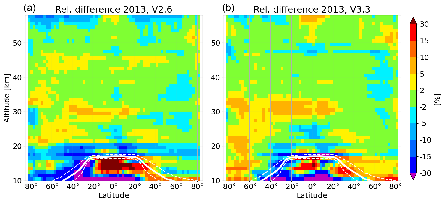
Figure 1 Relative mean differences between IUP-OMPS and MLS version 4.2 ozone profiles as a function of altitude and latitude for 2013. Panel (a) shows the comparison for IUP-OMPS V2.6 and panel (b) for IUP-OMPS V3.3. The thick white line marks the tropopause height and the dashed line its standard deviation.

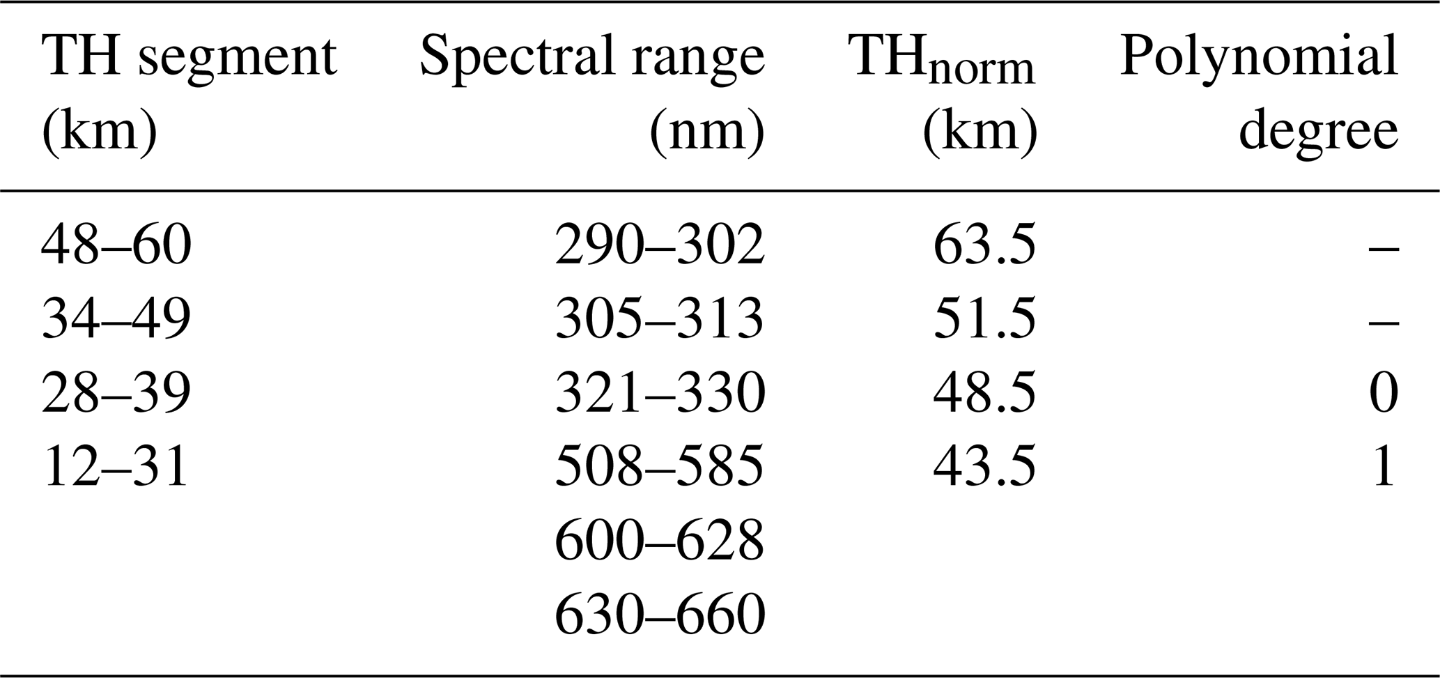
This study uses OMPS ozone profiles version 3.3 (IUP-OMPS V3.3). Comprehensive validation of the ozone profiles and details about the retrieval can be found in Arosio et al. (2018) and Arosio (2019) for the previous retrieval version (here named IUP-OMPS V2.6). The main differences between V2.6 and V3.3 are in the usage of the spectral segments and normalization THs. Table 1 lists the TH ranges, respective spectral segments selected for the retrieval, TH used for the normalization, and the order of the polynomials used for V3.3. Figure 1 presents a comparison of ozone profiles from the Microwave Limb Sounder (MLS) with IUP-OMPS V2.6 (left panel) and V3.3 (right panel) data. Both panels show relative differences between IUP-OMPS and the MLS L2 version 4.2 data as a function of altitude and latitude. Differences within ±10 % are observed above 20 km for both IUP-OMPS versions. Below 20 km, the differences can reach ±30 %. An overall reduction of the bias is found for IUP-OMPS V3.3, with main improvements in the lower tropical stratosphere and between 35 and 50 km. However, the bias increases between 30 and 35 km from 20° N to the south and below 20 km polewards of 60° S.

Table 1 Details of the IUP-OMPS ozone profile retrieval V3.3: TH segments, corresponding spectral ranges, and the order of the subtracted polynomial (dash means that no polynomial is subtracted). Tangent heights TH_norm are used to normalize the radiance in the given spectral range.

Our OMPS-LP ozone profile time series V2.6 and V3.3 use L1 V2.5 data. As discussed by Kramarova et al. (2018), the ozone time series above 20 km retrieved using this L1 data exhibit significant positive drift, especially after 2016. Our later investigations show that the data after 2018 are affected even more strongly. For this reason, we decided not to continue updating the OMPS-LNM-TrOC dataset beyond the end of 2018 using profiles based on L1 V2.5 data. Currently, only measurements from the central slit are used to retrieve ozone profiles because of remaining calibration issues related to the measurements from the side slits. More information and technical details on OMPS-LP can be found in Kramarova et al. (2018), Arosio et al. (2018), and references therein. A reprocessing of the OMPS-LNM-TrOC data is planned as soon as the new version of OMPS-LP stratospheric profiles (V4.0) based on the improved L1 data (V2.6) is available.

2.3 Tropopause height

In order to derive the stratospheric column from the retrieved ozone profile, the tropopause height (TPH) needs to be determined. The stratospheric column is then calculated by integrating the ozone profile from the tropopause up to the top of atmosphere, here, to the uppermost retrieval altitude of 60.5 km.

The most commonly used definition of the tropopause is the thermal or lapse-rate tropopause. WMO (1957) defines the thermal TPH as the lowest altitude level at which the lapse rate is less than or equal to 2 K km⁻¹, provided the average lapse rate between this level and all higher levels within 2 km also does not exceed this threshold. A drawback of this definition is that it might fail in polar regions if the stratosphere is very cold. Alternatively, the dynamic tropopause can be used, which is defined by the potential vorticity (PV), which increases with altitude. Different studies suggest this tropopause altitude to be between 1 and 4 PVU (potential vorticity unit; 1 PVU = 1.0 × 10⁶ km² kg⁻¹ s⁻¹) (Hoinka, 1998). This tropopause definition is, however, only applicable in the extra-tropics.

In this study, a blended tropopause definition is employed: the thermal tropopause is used in the tropics, between 20° N and 20° S, while the altitude level with a PV of 3.5 PVU (Zängl and Hoinka, 2001) is selected as TPH for latitudes above 30°. In the transition zone, between 20 and 30° latitude in each hemisphere, the TPH is calculated by averaging the thermal and the dynamical values weighted with the distance to the regime boundaries. This approach is consistent with the TPH definition employed in Ebojie et al. (2014) and Jia (2016) to obtain tropospheric ozone from SCIAMACHY using the limb–nadir Matching technique.

For every IUP-OMPS ozone profile location and time, the thermal and the dynamic TPHs are determined using the ECMWF ERA-5 reanalysis data (Hersbach et al., 2020). The ECMWF ERA-5 data have a spatial resolution of 0.75° × 0.75° and a temporal sampling of 6 h. The data are linearly interpolated using the four data points around the exact given location for the two closest times to obtain the TPH at the precise time and place of every limb state.

3 Obtaining tropospheric ozone columns from OMPS-NM/OMPS-LP LNM

Employing the LNM technique, the tropospheric ozone product is generated for matched observations as follows:

$$\begin{array}{}\text{(1)}& \mathrm{TrOC}=\mathrm{TOC}-\mathrm{SOC}.\end{array}$$

This means that the SOC, calculated from IUP-OMPS ozone profiles, is subtracted from TOC, retrieved from OMPS-NM using the WFFA approach. The latter retrieval is done only for those across-track ground pixels that are collocated to the location of the TP of the limb ozone profiles (usually around the centre of the swath). Both retrievals are completely independent of each other. For a consistency reason, they use the same ozone absorption cross-sections (Serdyuchenko et al., 2014). Details on the matching procedure, which identifies the collocated ground pixels, are given below.

Although the IUP-OMPS ozone profiles are available from 8.5 to 60.5 km altitude, only ozone values above 12.5 km are considered because of a large retrieval uncertainty of the limb profiles below this altitude (Arosio et al., 2018). If the TPH calculated as described in Sect. 2.3 is below 12.5 km, the ozone vertical distribution between TPH and 12.5 km is taken from the IUP-2018 ozone profile climatology (Orfanoz-Cheuquelaf et al., 2021). This climatology classifies ozone profiles as a function of season, latitude, and total ozone column. The climatological profile is offset by a scalar value which is given by the difference between the observed and climatological ozone at 12.5 km.

Subsequently, cloud flags provided along with the ozone profiles are analysed. The complete profile is rejected if clouds above the TPH are detected. After passing the cloud filter, a vertical resolution quality filter is applied, which considers the mean and the standard deviation of the vertical resolutions of all profiles observed within a given calendar year. If the vertical resolution of a single ozone profile at any altitude between 12.5 and 60.5 km deviates by more than 2 standard deviations from the yearly mean, the entire profile is rejected.

The SOC in DU is determined then by integrating the O₃ concentration from the TPH to 60.5 km, as follows:

$$\begin{array}{}\text{(2)}& \mathrm{SOC}={\displaystyle \frac{\mathrm{1}}{\mathrm{2}}}\sum _{i\left(\mathrm{TPH}\right)}^{i\left(\mathrm{60.5}\mathrm{km}\right)-\mathrm{1}}{\displaystyle \frac{\left(c_{i+\mathrm{1}}+c_i\right)\left(z_{i+\mathrm{1}}-z_i\right)}{\mathrm{2.6867}\times {\mathrm{10}}^{\mathrm{11}}}},\end{array}$$

where i is the index of the altitude level, c the ozone number density in units of molecules cm⁻³, and z the altitude in units of kilometres.

The LNM procedure is illustrated in Fig. 2. The grid cells plotted in the figure correspond to the ground pixels of OMPS-NM, and the red points represent the tangent height footprint of the OMPS-LP states. The matching is done as follows. For each OMPS-LP state location (red points), the OMPS-NM ground pixel that contains the location of TPs is identified (orange box in Fig. 2), and two neighbouring across-track pixels (yellow boxes) are also selected to obtain a mean TOC. The matching procedure also considers all triple pixels between consecutive limb states (e.g. a row of three yellow boxes). If the OMPS-NM pixels are located between consecutive OMPS-LP states, the final SOC value to be subtracted is obtained by interpolating between the SOCs from the two bracketing limb states. Finally, the subtraction SOC from TOC is performed to yield TrOC. The final size of the TrOC pixels is approximately 50 km along track and 150 km across track. For the calculation of the three-pixel mean TOC, only cloud-free OMPS-NM pixels (cloud fraction below 0.1) are used to calculate the three-pixel mean TOC. If a single cloudy pixel is detected, this one is neglected, and the average is performed. The entire matching is rejected in the case of two or more cloudy TOC pixels.

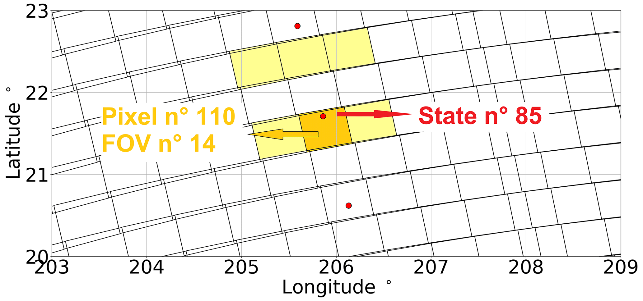
Figure 2 Example of the matching between OMPS-NM and OMPS-LP observation scenes. The red points mark the footprints of tangent points (TPs) of the limb observations. The grid cells represent the ground pixels of OMPS-NM. The yellow boxes indicate the nadir ground pixel averaged to obtain the TOC assuming the nadir pixels are cloud-free. The orange box marks the exact match between the OMPS-NM ground pixel number 110 (along track) in position 14 (across track) with the OMPS-LP observation number 85 (state).

4 OMPS-LNM uncertainties

Uncertainties from the ozone total column and profile retrievals contribute to the uncertainty of the tropospheric ozone data. An additional contribution comes from the uncertainty in the tropopause height calculation. The overall TrOC uncertainty is estimated by combining these three components in a Gaussian sum as follows:

$$\begin{array}{}\text{(3)}& X_{\mathrm{TrOC}}=\sqrt{X_{\mathrm{TOC}}^{\mathrm{2}}+X_{\mathrm{SOC}}^{\mathrm{2}}+X_{\mathrm{TPH}}^{\mathrm{2}}},\end{array}$$

where X_TrOC, X_TOC, X_SOC, and X_TPH are the uncertainties estimated for the tropospheric ozone column, total ozone column, stratospheric ozone column, and tropopause height, respectively, all expressed in DU. All values reported in this section are assumed to be 1σ uncertainties and represent the uncertainty of a single observation.

The analysis in this study distinguishes between random and systematic uncertainties, with random components contributing to the variance of the data and systematic components contributing to the bias. In the following, details on the terms on the right-hand side of Eq. (3) are discussed.

4.1 Total ozone column uncertainty

The full analysis of uncertainties related to the WFDOAS technique is detailed in Coldewey-Egbers et al. (2005). Due to differences in the spectral window size and the polynomial degree, the uncertainty analysis was repeated for the WFFA technique for some parameters as reported in Orfanoz-Cheuquelaf et al. (2021). For some other parameters, the uncertainties derived from the WFDOAS technique were also considered valid for WFFA. Table 2 summarizes individual contributions to the overall TOC uncertainty from the analysis presented in Coldewey-Egbers et al. (2005) and Orfanoz-Cheuquelaf et al. (2021).

Table 2 Summary of contributions to the uncertainty of the total ozone column.

^a Orfanoz-Cheuquelaf et al. (2021). ^b Coldewey-Egbers et al. (2005).

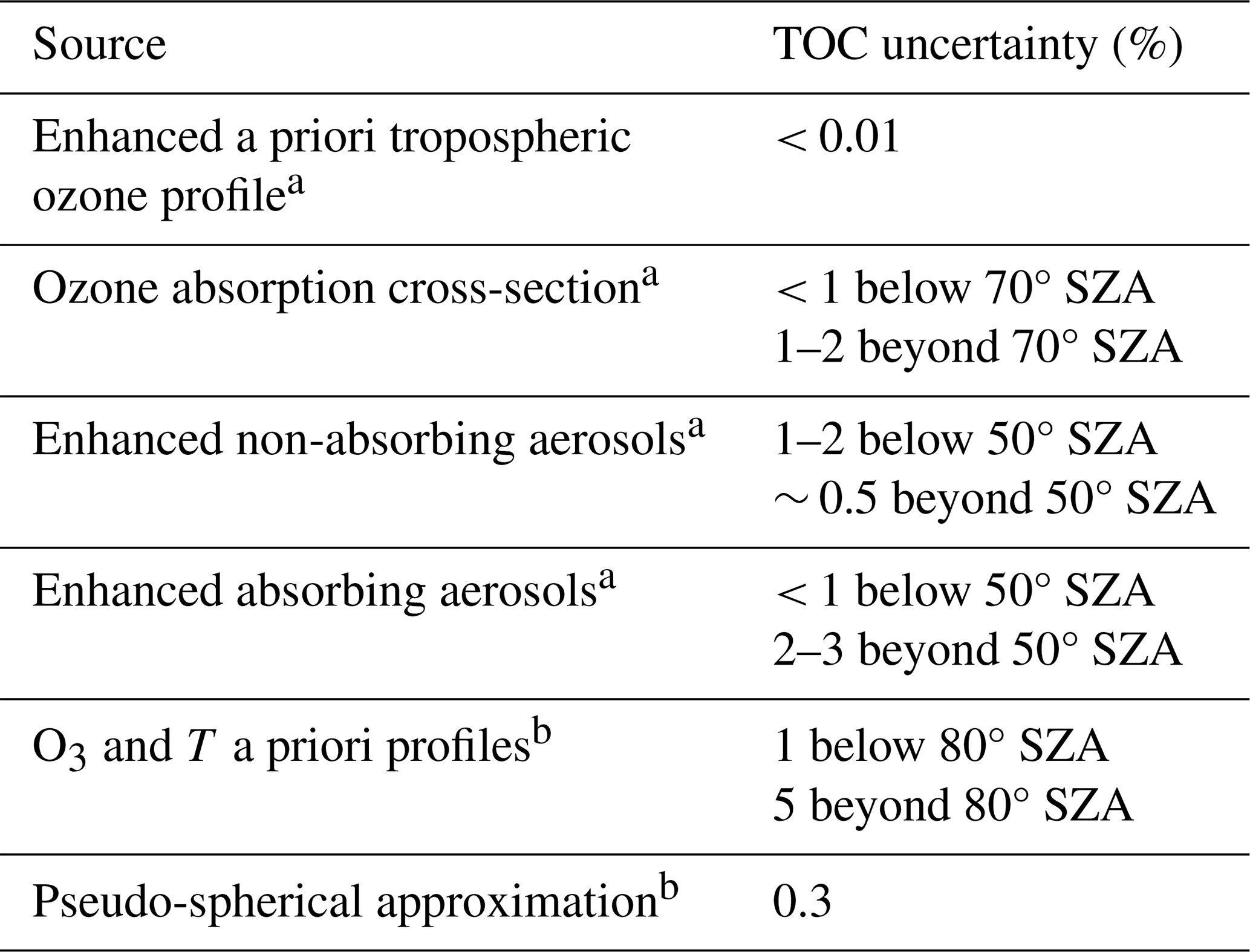
In particular, for the case of increasing the tropospheric ozone a priori profile by a factor of 5, the uncertainty in TOC is less than 0.01 %. For different absorption cross-sections (Brion, Malicet, and Daumon in Malicet et al., 1995, vs. Serdyuchenko in Serdyuchenko et al., 2014), the uncertainty is less than 1 % for SZAs below 70° and increases to 2 % for higher SZAs. For scenes with enhanced boundary layer aerosols at SZAs below 50°, the uncertainties are between 1 % and 2 % for non-absorbing aerosols and less than 1 % for absorbing aerosols. For SZAs beyond 50°, the uncertainties are about 0.5 % for non-absorbing aerosols and between 2 % and 3 % for absorbing aerosols. For ozone and temperature a priori profiles, the uncertainty is 1 % for SZAs under 80°. The use of the pseudo-spherical approximation results in an uncertainty of 0.3 %.

From the contributions listed in Table 2, the only systematic component is the uncertainty associated with the absorption cross-section, which results in a systematic uncertainty of TOC of about 1 %. The total random component is calculated by summing up all other contributions using the Gaussian rule. This results in a random uncertainty of 1.8 %–3.8 %, where the range is mostly dominated by the aerosol scenarios, particularly in extreme cases. A typical random uncertainty is estimated to be about 2.8 %. For a typical total ozone amount of about 300 DU (Rowland et al., 1988), the random uncertainty of 2.8 % translates into 8.4 DU, and the systematic uncertainty of 1 % into 3 DU.

4.2 Stratospheric ozone column uncertainty

A comprehensive discussion of the uncertainty budget for the IUP-OMPS ozone profiles was presented by Arosio et al. (2022). Uncertainties due to retrieval noise and from the retrieval parameters, i.e. parameters that do not enter the measurement vector, are quantified using synthetic retrievals and extensively discussed in the above mentioned study. Uncertainties originating from model approximations and spectroscopic data are also investigated. A representative set of OMPS-LP geometries was selected to provide a reliable estimation of the uncertainties as a function of latitude and season.

To assess the SOC uncertainty based on the available uncertainty budget for ozone profiles, first, we need to discuss the behaviour of the uncertainty components in the altitude domain. In this study, we consider the uncertainties of the pressure, temperature, and aerosol extinction coefficient to be predominantly systematic in the altitude domain. This is because the former two parameters are taken from the GEOS-5 model data, whose uncertainties originate from the model assumptions with more probable large-scale influence rather than from random noise-like errors. Concerning the stratospheric aerosol extinction coefficients, our experience is that dominating errors in their retrievals mostly scale the resulting vertical profiles. The retrieval-noise-related uncertainty is considered uncorrelated with altitude; i.e. it is randomly distributed in the vertical domain. As a consequence, the following formulas have been used to calculate the SOC uncertainty from the profile values:

$$\begin{array}{}\text{(4)}& {\displaystyle }{\mathit{\sigma }}_{\mathrm{SOC},\mathrm{correlated}}=\sum _z{\mathit{\sigma }}_{{\mathrm{O}}_{\mathrm{3}}}\left(z\right)/\sum _z{\mathrm{O}}_{\mathrm{3}}\left(z\right)\text{(5)}& {\displaystyle }{\mathit{\sigma }}_{\mathrm{SOC},\mathrm{uncorrelated}}=\sqrt{\sum _z{\left({\mathit{\sigma }}_{{\mathrm{O}}_{\mathrm{3}}}\left(z\right)\right)}^{\mathrm{2}}}/\sum _z{\mathrm{O}}_{\mathrm{3}}\left(z\right),\end{array}$$

where O₃ and ${\mathit{\sigma }}_{{\mathrm{O}}_{\mathrm{3}}}$ are, respectively, the reference ozone concentrations and their uncertainties as functions of altitude z. The second equation was only applied for the uncertainty from retrieval noise.

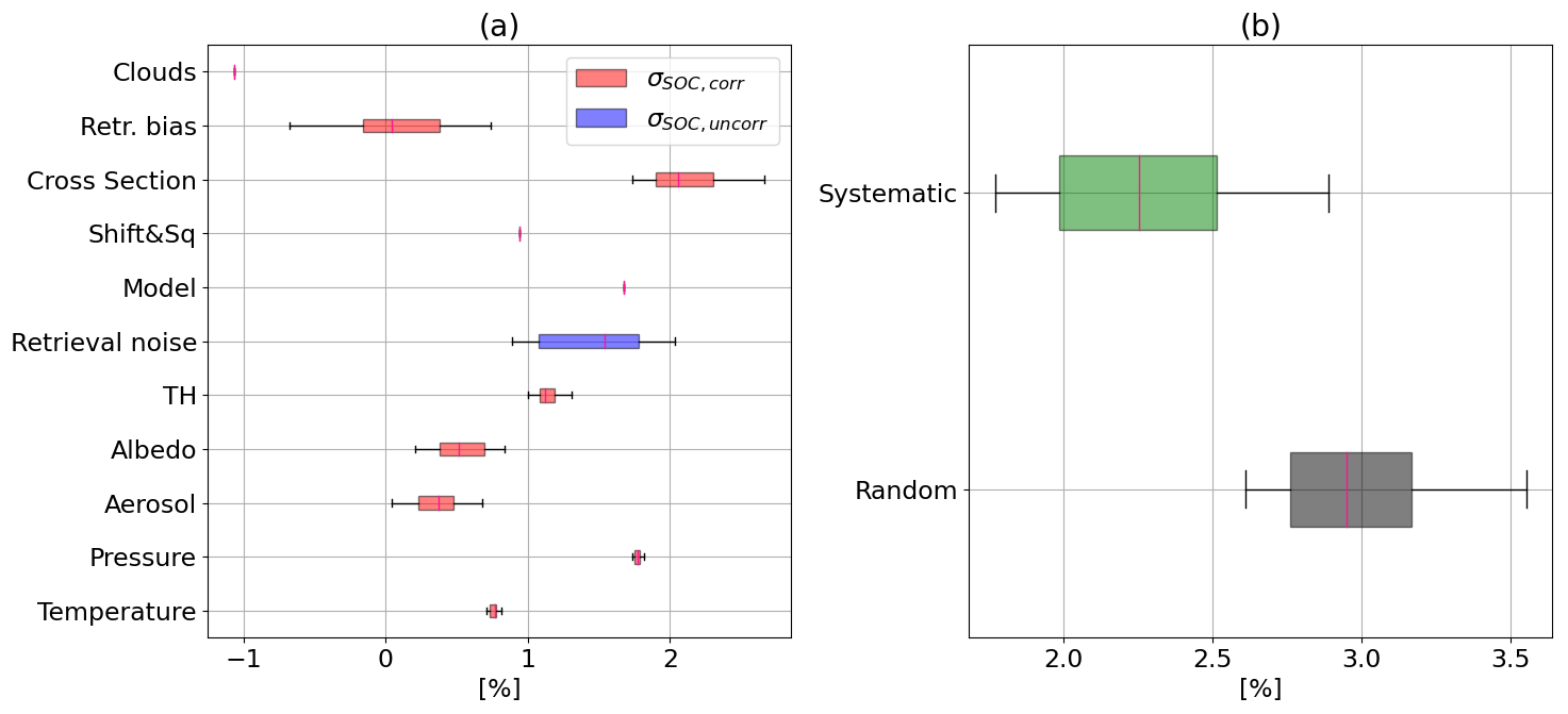
Figure 3 Contributions to SOC uncertainty. (a) SOC uncertainties from different sources. (b) Total random and systematic uncertainty for SOC. The error bars span the outlier ranges, the boxes span the range between the first and third percentiles, and the magenta middle lines refer to the median values.

The SOC uncertainty contributions estimated from a selected representative set of geometries (Arosio et al., 2022) are shown in Fig. 3a, where different colours indicate the usage of Eq. (4) (blue) or Eq. (5) (red), respectively. Uncertainties related to the cloud impact, the radiative transfer model, and the use of the spectral shift-and-squeeze correction in the pre-processing routine (“Shift&Sq”) are independent of the viewing geometry, so that a single value is available. For other contributions, the statistics within the data sample are shown. The contribution from cloud artefacts is based on Fig. 10a of Arosio et al. (2022), assuming that thin tropospheric clouds can still affect the retrieval bypassing the 0.1 cloud fraction threshold imposed on the nadir pixel (total column ozone) in the matching procedure.

The total random SOC uncertainty was calculated by applying the Gaussian sum:

$$\begin{array}{}\text{(6)}& {\mathit{\sigma }}_{\mathrm{SOC},\mathrm{random}}=\sqrt{\begin{array}{c}{\mathit{\sigma }}_{\mathrm{SOC},P}^{\mathrm{2}}+{\mathit{\sigma }}_{\mathrm{SOC},T}^{\mathrm{2}}+{\mathit{\sigma }}_{\mathrm{SOC},\mathrm{alb}}^{\mathrm{2}}+\\ +{\mathit{\sigma }}_{\mathrm{SOC},\mathrm{aer}}^{\mathrm{2}}+{\mathit{\sigma }}_{\mathrm{SOC},\mathrm{TH}}^{\mathrm{2}}+{\mathit{\sigma }}_{\mathrm{SOC},\mathrm{retr}.\mathrm{noise}}^{\mathrm{2}}\\ +{\mathit{\sigma }}_{\mathrm{SOC},\mathrm{S}\mathrm{\&}\mathrm{S}}^{\mathrm{2}}\end{array}},\end{array}$$

where the various terms on the right-hand side denote the individual components related to the retrieval parameters, i.e. pressure (σ_SOC,P), temperature (σ_SOC,T), surface albedo (σ_SOC,alb), aerosol extinction (σ_SOC,aer) and TH (σ_SOC,TH) correction, and to both the retrieval noise (${\mathit{\sigma }}_{\mathrm{SOC},\mathrm{ret}.\mathrm{noise}}$) and the shift-and-squeeze correction (σ_SOC,S&S).

The total systematic uncertainty was computed as follows:

$$\begin{array}{}\text{(7)}& {\mathit{\sigma }}_{\mathrm{SOC},\mathrm{systematic}}=\sqrt{\begin{array}{c}\left({\mathit{\sigma }}_{\mathrm{SOC},\mathrm{retr}.\mathrm{bias}}+{\mathit{\sigma }}_{\mathrm{SOC},\mathrm{clouds}}+\right.\\ {\left.{\mathit{\sigma }}_{\mathrm{SOC},\mathrm{model}}\right)}^{\mathrm{2}}+{\mathit{\sigma }}_{\mathrm{SOC},\mathrm{cross}\mathrm{section}}^{\mathrm{2}}\end{array}},\end{array}$$

where the terms with known signs are first summed up, i.e. the uncertainties related to the retrieval bias (${\mathit{\sigma }}_{\mathrm{SOC},\mathrm{retr}.\mathrm{bias}}$), cloud artefacts (σ_SOC,clouds), and radiative transfer model approximations (σ_SOC,model). Finally, the root mean square with the cross section term (σ_{SOC,cross section}) is calculated.

The total systematic and random SOC uncertainties are illustrated in Fig. 3b. Their typical values are about 2.0 %–2.5 % and 2.8 %–3.2 %, respectively. Medians of 2.2 % for the systematic and 3 % for the random uncertainties are used below to calculate the final uncertainty of TrOC. Considering that stratospheric ozone contributes approximately 90 % to the total ozone, and the global average of the total ozone is 300 DU, the global average of SOC is about 270 DU. Thus, the systematic uncertainty of 2.2 % translates to 5.9 DU and the random uncertainty of 3 % to 8 DU.

4.3 Tropopause height uncertainty

The calculated TPH introduces another uncertainty in the retrieved TrOC. Besides the natural variability of the TPH and the particular definition used to determine it, the uncertainty depends on the vertical resolution of the reanalysis data used to determine TPH, here the ECMWF ERA-5 dataset. The ERA-5 reanalysis data are provided at pressure levels, and derived quantities such as the PV are defined at the centre of the layers bordering the pressure levels. To determine the tropopause altitude (in km), the pressure levels are converted into geometrical heights. In this domain, the vertical sampling of the ERA-5 dataset varies with altitude ranging from 270 to 400 m between 5 and 20 km altitude.

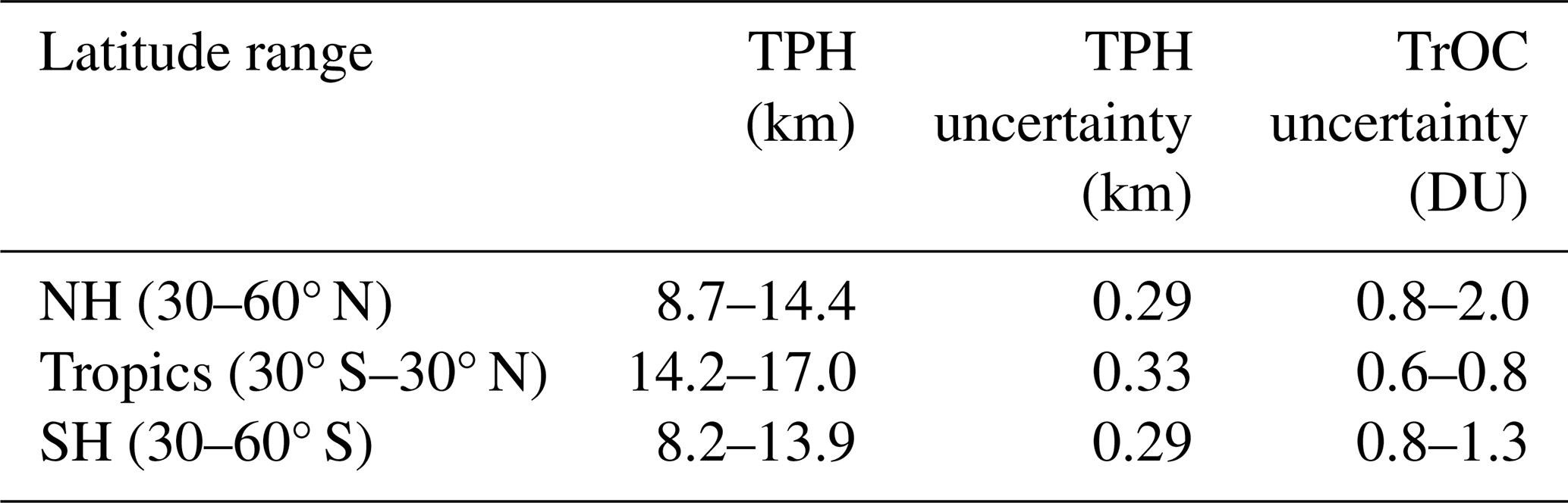
The TPH uncertainty as a function of latitude is determined by the vertical extent of the ERA-5 layer containing the TPH and is estimated using the zonal mean (climatology) of the TPH to be 0.29 km in the Northern Hemisphere, 0.33 km in the tropics, and 0.29 km in the Southern Hemisphere. To calculate the effect on TrOC, these uncertainties were added to and subtracted from the TPH in the OMPS-LNM processing chain. The TPH range, their uncertainties, and the final contributions to the TrOC uncertainty are presented in Table 3 for three zonal bands. In the Northern Hemisphere (NH), the mean uncertainty in TrOC ranges from 0.8 to 2 DU, in the tropics from 0.6 to 0.8 DU, and in the Southern Hemisphere (SH) between 0.8 and 1.3 DU.

Table 3 Uncertainties related to TPH for the Northern Hemisphere, tropics, and Southern Hemisphere.

4.4 Final tropospheric ozone column uncertainties

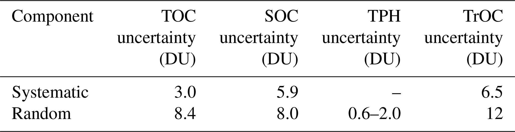
The systematic and random components of the final TrOC uncertainty are calculated using Eq. (3), and the results are summarized in Table 4. The TPH contribution is considered random. Although a range of values was obtained for the TPH uncertainty, this variation does not impact the final results. The final TrOC uncertainties do not vary significantly with latitude. The overall random and systematic uncertainties of OMPS-LNM TrOC are about 12 and 6.5 DU, respectively.

Table 4 Estimated uncertainties for TOC, SOC, TPH and TrOC.

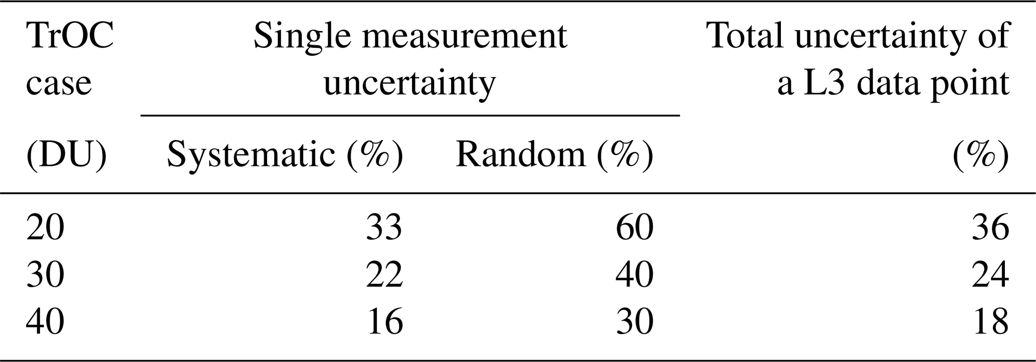
The standard Level 3 product of the OMPS-LNM is a monthly mean gridded (0.5°×1.5° (latitude–longitude)) dataset. The overall uncertainty for a typical Level 3 data point can be estimated as follows:

$$\begin{array}{}\text{(8)}& {\mathit{\sigma }}_{{\mathrm{TrOC}}_{\mathrm{L}\mathrm{3}}}=\sqrt{X_{{\mathrm{TrOC}}_{\mathrm{syst}}}^{\mathrm{2}}+{\displaystyle \frac{X_{{\mathrm{TrOC}}_{\mathrm{random}}}^{\mathrm{2}}}{N}}},\end{array}$$

where N is the number of observations averaged within a grid cell; in our case, it is about 14. The total uncertainty for a typical Level 3 data point is then estimated to be 7.2 DU. The corresponding uncertainties in percentage are provided in Table A1 for representative TrOC values of 20, 30, and 40 DU.

5 OMPS-LNM tropospheric ozone evaluation

In this section, the OMPS-LNM TrOC dataset is described and compared with ozonesondes and other satellite datasets, here OMI/MLS TOR and TROPOMI CCD. For the evaluation, the OMPS-LNM TrOC data were mapped onto a regular daily grid of 0.5° × 1.5° (latitude–longitude) from 60° S to 60° N.

5.1 Seasonal analysis

Figure 4 shows seasonal maps of OMPS-LNM TrOC. The region of the South Atlantic Anomaly (SAA) is marked on the map. This is an anomaly of the Earth’s geomagnetic field (Pavón-Carrasco and De Santis, 2016) that affects satellite electronics and perturbs measurements. After applying the quality filters, the data density is significantly reduced within the SAA.

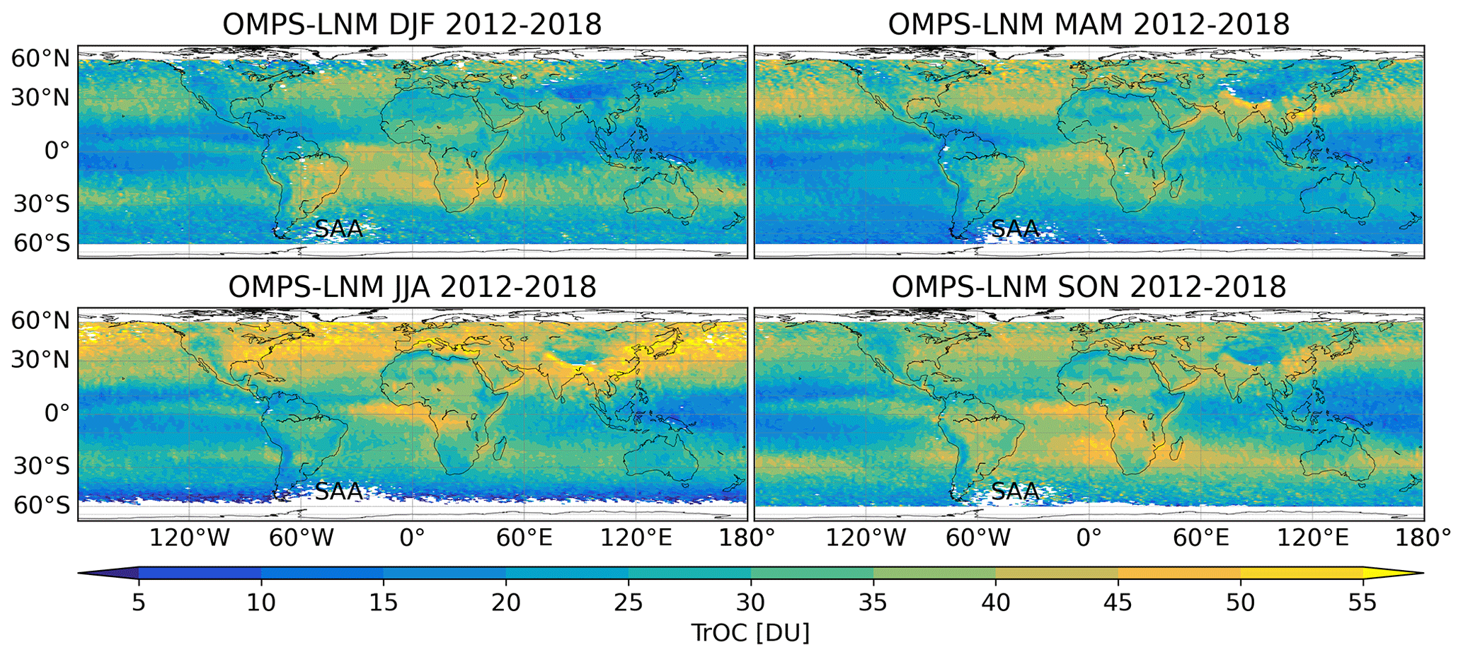
Figure 4 Seasonal maps of OMPS-LNM TrOC averaged from 2012 to 2018.

A band of higher values is observed between 0 and 10° N in the Pacific Ocean during all seasons and in the Atlantic Ocean during boreal summer (JJA) and autumn (SON). This feature is not seen in other satellite datasets and will be discussed in more detail in Sect. 5.2.

The seasonal tropospheric ozone maps show, apart from the above-mentioned issue, typical features reported before. Higher values in the extratropical hemispheric spring/summer are observed, coinciding with the likely increase in the photochemical production of tropospheric ozone (Logan, 1985; Monks et al., 2015; Gaudel et al., 2018). Low ozone is observed throughout the year in high-topography areas like the Andes and the Himalayas. Minimum ozone is observed above Indonesia, extending into the Pacific Ocean.

Most of the year, high values are observed in the southern subtropical Pacific Ocean (20–30° S), attributed to biomass burning and stratospheric intrusions (Daskalakis et al., 2022). Higher values are observed above east Asia and the northern subtropical Pacific in all seasons, with maxima during boreal spring/summer. In addition to increased photochemical production of ozone during spring/summer, these high values might be caused by stratospheric intrusions above the ocean around 30° N (Oltmans, 2004) and outflow from intensive biomass burning in continental southeast Asia contributing during winter and spring (Liu et al., 1999).

High values, largest during boreal summer and lower during boreal autumn/winter, are observed over the subtropical North Atlantic throughout the year. During winter, high values are associated with the long-range transport of precursors from anthropogenic emissions in North America (Cuevas et al., 2013). In addition to photochemical production, stratospheric intrusions (Škerlak et al., 2014) and lighting (Cooper et al., 2009) are important contributors during the summer. Over the tropical Atlantic Ocean, lightning contributes to tropospheric ozone increase (Jenkins and Ryu, 2004). During austral spring/summer, the maximum over the southern Atlantic Ocean results from contributions of biomass burning in Africa and South America, as well as from NO_x soil sources (Sauvage et al., 2007). High values above the South Indian Ocean are associated with biomass burning in Africa, particularly during austral spring, in addition to stratospheric intrusions (Fishman et al., 1991; Liu et al., 2017). The seasonality observed over the Arabian Sea is consistent with the analysis presented by Jia et al. (2017).

5.2 Band of high ozone over the northern tropical Pacific and Atlantic oceans

A band of fairly high tropospheric ozone columns over the Pacific and Atlantic oceans is seen in OMPS-LNM data between the Equator and 10° N. Such a band is not observed by satellite datasets which use nadir ozone profiles (Ohyama et al., 2012), the CCD method (Valks et al., 2014; Leventidou et al., 2016; Hubert et al., 2021), or residual techniques employing occultation or limb-emission measurements (Fishman et al., 2003; Ziemke et al., 2006). However, this particular feature is observable in the LNM dataset from SCIAMACHY (Jia, 2016) and in the NASA product from OMPS (Ziemke et al., 2019a). This indicates that it is most likely a feature specific to the residual technique employing limb-scatter measurements.

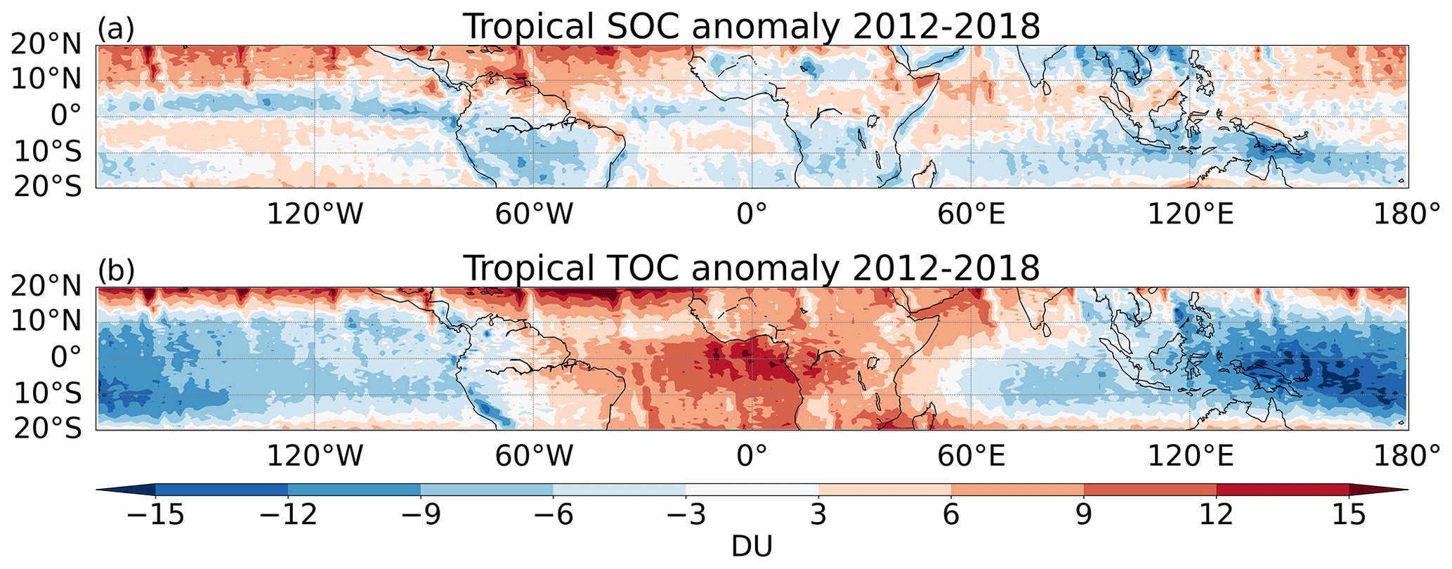
Figure 5 OMPS-LNM tropical anomalies of (a) SOC and (b) TOC from 2012 to 2018.

Figure 5 shows maps of TOC and SOC anomalies from the OMPS-LNM TrOC analysis between 20° S and 20° N. The anomalies were computed by subtracting the long-term mean from all data in the tropics. The SOC anomalies (Fig. 5a) show lower values over the Pacific and Atlantic, matching the band of high TrOC (Fig. 4). This feature is not evident in the TOC anomalies (Fig. 5b). A seasonal analysis of the SOC anomalies (not shown here) shows that this feature is persistent throughout the year and only slightly weaker during boreal summer. The negative bias in SOC leads to a high bias in the tropospheric ozone of about 10 DU (see Fig. 4). We conclude that this feature is likely an artefact from the limb ozone profiles.

Among other parameters, the surface reflectivity field retrieved along with the ozone profiles from OMPS-LP was analysed to investigate the cause of the unusually low OMPS-LP SOC. An area with higher surface reflectivity between the Equator and 10° N over the Pacific and Atlantic oceans correlates with the anomalous band. The enhanced surface albedo band is shifted a few degrees northwards and is somewhat wider than the tropospheric ozone and SOC anomaly bands. The enhanced surface reflectivity band matches the position of the Intertropical Convergence Zone (ITCZ). Even though the LNM tropospheric ozone used only ozone profiles free of clouds above the tropopause and nadir pixels with cloud fraction below 0.1, the influence of the ITCZ on TrOC is evident.

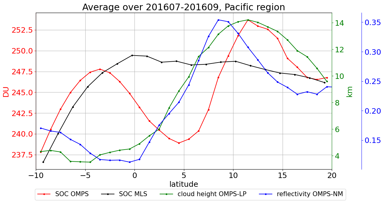
Figure 6 Latitudinal dependence of the July–September 2016 SOC average over the Pacific Ocean from OMPS (red) and MLS (black) and the mean cloud-top height (green) and mean surface reflectivity (blue).

Figure 6 shows the latitudinal dependence of the July–September 2016 average SOC over the Pacific Ocean from OMPS-LP (red) and MLS (black), the cloud-top height (green) from OMPS-LP, and the surface reflectivity (blue) retrieved from OMPS-NM. It is seen that the cloud-top height significantly increases north of the Equator, and the reflectivity increases as well. A correlation between OMPS SOC and the reflectivity gradient is observed. When the gradient in the reflectivity is maximum, the OMPS SOC reaches a minimum, decreasing by around 10 DU relative to MLS. OMPS SOC recovers rapidly as the gradient in the reflectivity changes. The MLS SOC does not show any dependence on the presence of clouds.

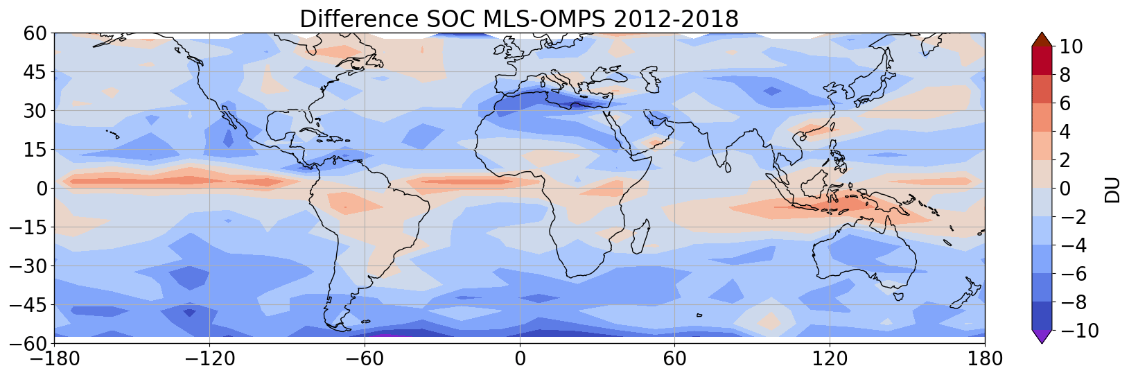
Figure 7 Mean differences in SOC from MLS and IUP OMPS-LP profiles from 2012 to 2018.

In a more extensive comparison between SOC from OMPS-LP and MLS, Fig. 7 shows the global difference between the datasets for the entire period 2012–2018. The band of lower SOC from OMPS-LP in the Pacific and Atlantic oceans is clearly seen. Also, a larger difference is observed between Australia and the Equator. Larger OMPS-LP values are seen in the southern Mediterranean Sea and in the transition zone between the bright desert and the dark sea. The current hypothesis is that a strong gradient in the surface reflectivity along the instrument line of sight (LOS) is not properly accounted for in the limb retrieval and generates artefacts in the retrieved ozone profiles. This affects all limb-scatter retrievals: IUP-OMPS, SCIAMACHY and NASA OMPS-LP. An investigation of the influence of the horizontal gradient in the reflectivity of the underlying scene on one-dimensional limb profile retrievals is out of the scope of this research. However, it is important to be aware of this influence on the OMPS-LNM tropospheric ozone.

5.3 Comparison with ozonesondes

Ozonesonde data from WOUDC (Fioletov et al., 1999) and SHADOZ V6 (Witte et al., 2017; Thompson et al., 2017) were used in this study. The procedure to create the collocated OMPS-LNM dataset was optimized to obtain a sufficient number of comparisons. For each ozonesonde profile, OMPS-LNM data from the grid cell enclosing the launch site and all immediately adjacent grid cells were averaged (without any weighting) to create the collocated OMPS dataset. The temporal averaging included OMPS-LNM data from the day of the ozonesonde launch and 1 d before and 1 d after the launch. Only ozonesonde sites with collocated OMPS data of at least 55 d during the entire comparison period (2012–2018) were considered. In total, 22 sites were available, 8 from SHADOZ and 14 from WOUDC. The total number of collocated days is rather low for 7 years because the daily coverage of OMPS-LNM is sparse, and ozonesondes are launched four times per month at maximum.

Figure 8 shows time series of ozonesonde (red) and collocated OMPS-LNM (black) tropospheric ozone columns for three selected sites: Madrid in the Northern Hemisphere (40.5° N, 3.7° W), Hilo in the tropics (19.4° N, 155.4° W), and Broadmeadows in the Southern Hemisphere (37.7° S, 145° E). The seasonality and variability shown by both datasets are in good agreement. The bias between the datasets is −0.8, −3.5, and −1.9 DU, respectively, with OMPS-LNM being generally lower than the sondes. The standard deviation of the difference is around 8.5 DU for each site. No clear dependence on latitude is identified from the analysis of differences between the OMPS-LNM and ozonesonde data for all sites (not shown here).

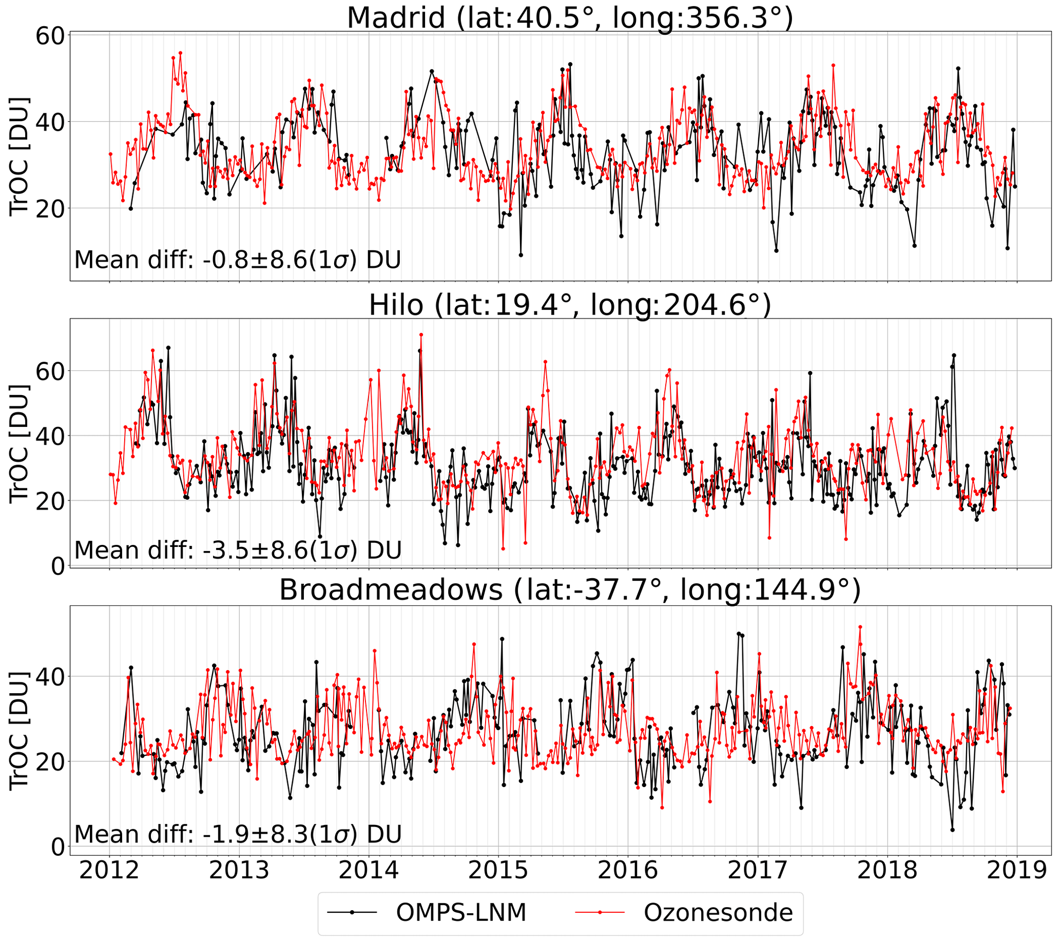
Figure 8 Time series of tropospheric ozone column from individual ozonesonde measurements (red) and daily averaged collocated OMPS-LNM (black) data for three selected sites.

Table 5 Comparison of TrOC from collocated ozonesonde and OMPS-LNM measurements between 2012 and 2018. The ozonesonde site location, mean values, and standard deviations of the datasets are listed. It also includes the mean difference (OMPS-LNM − ozonesonde) and the relative difference between the datasets (mean diff. $/$ mean(ozonesonde) × 100).

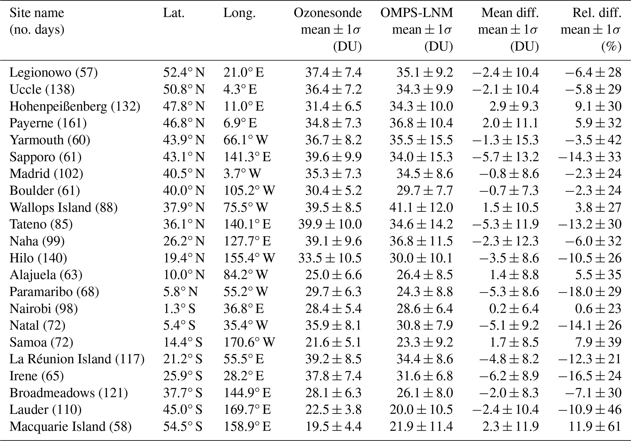
Table 5 summarizes the collocated mean value from the ozonesondes and OMPS, their standard deviation, and the mean difference (average of OMPS-LNM minus ozonesonde time series) between the datasets for all sites. The table's first column shows the site's name and the number of collocated days. No dependency on the number of collocated days is observed. Typically, the standard deviations for OMPS-LNM are higher than those for ozonesondes by about 2.7 DU. Larger differences in the standard deviation are found for Yarmouth, Lauder, and Macquarie Island, where the standard deviations of OMPS-LNM are higher than those of the ozonesondes by 7.3, 6.6, and 6.6 DU, respectively. Some exceptions are Hilo, Natal, and Irene, where the standard deviations of the ozonesondes are higher than those for OMPS-LNM by 0.5, 0.3, and 0.5 DU respectively. The standard deviations of the differences range from 6.4 DU for Nairobi to 15 DU for Yarmouth. The bias between the datasets ranges from −6.2 DU for Irene to 2.9 DU for Hohenpeissenberg. The mean bias between OMPS-LNM and ozonesondes is found to be −1.7 ± 2.8 DU. Out of 22 sites, 7 exhibit a positive bias. A total of 11 sites show a bias within ±2 DU.

5.4 Comparison with OMI/MLS TOR and TROPOMI CCD datasets

The OMI/MLS TOR product is a tropospheric ozone dataset retrieved using the TOR technique with TOC from OMI and SOC from MLS profiles observed since 2004 (Ziemke et al., 2006). Both instruments are aboard the Aura satellite. Measurements of MLS are taken approximately 7 min before OMI. The OMI/MLS TOR product is available as monthly mean values on a 1°×1.25° (latitude–longitude) grid at https://acd-ext.gsfc.nasa.gov/Data_services/cloud_slice/new_data.html​​​​​​​ (last access: 5 January 2023). The monthly means are obtained by subtracting daily means of SOC from TOC daily means and subsequent averaging. The TPH needed to determine SOC was obtained using the thermal definition of the tropopause from the NCEP reanalysis. A moving 2D (latitude–longitude) Gaussian function was used to fill gaps in SOC in the along-track direction, followed by a linear interpolation along the longitude. Daily global gridded maps were generated with 1° × 1.25° spatial sampling. OMI TOMS L3 TOC data were filtered for clear-sky conditions by keeping only measurements with reflectivity less than 0.3. A comparison of OMI/MLS TOR with ozonesondes from September 2004 to August 2005 showed a difference of around 2 DU, with OMI/MLS being higher than the ozonesondes (Ziemke et al., 2006). For the comparison here, the OMPS-LNM data were re-gridded onto the OMI/MLS grid (1° lat. × 1.25° long.) and averaged monthly.

The operational TrOC product from TROPOMI aboard S5P is derived with the CCD technique using the OFFL GODFIT V4 TOC (Hubert et al., 2021). The reference region, i.e. the region to estimate the above deep convective clouds column (ACCO), is the tropical eastern Indian and western Pacific oceans, 20° S–20° N, 70° E–170° W. The deep convective clouds are selected using a cloud fraction larger than 0.8, cloud albedo higher than 0.8, and effective cloud pressure less than 300 hPa. The ozone profile climatology of McPeters and Labow (2012) is used to estimate the ozone column from the retrieved cloud-top pressure to the reference level of 270 hPa. The final adjusted ACCO values are averaged over 5 d and 0.5° latitude bins and smoothed using a running mean over 2.5° latitude. The TOC from cloud-free pixels with cloud fraction less than 0.1 is averaged over 3 d and binned into a 0.5°×1° (latitude–longitude) grid. The ACCO is subtracted from TOC for each grid cell. The final TrOC from the ground to the 270 hPa level is sampled daily and represents a clear-sky 3 d running average (Hubert et al., 2021). Results of the validation of TROPOMI CCD by daily comparisons with SHADOZ ozonesondes from May 2018 to November 2021 are available online at http://mpc-vdaf-server.tropomi.eu/o3-tcl/o3-tcl-offl-ozone-sonde (last access: 20 March 2024). A positive bias was found for nine SHADOZ sites, with a mean bias of 3.2 DU and a standard deviation of 1.8 DU.

In order to compare OMPS-LNM with TROPOMI CCD data, the vertical coverage of the latter dataset was extended from the 270 hPa pressure level to TPH using the IUP-2018 ozone profile climatology. Furthermore, TROPOMI CCD data was re-gridded to the finer OMPS-LNM grid, considering only OMPS-LNM grid cells with data, and then averaged monthly.

Figure 9 shows the mean difference between OMPS-LNM and TROPOMI CCD from May to December 2018 (top) and between OMPS-LNM and OMI/MLS from 2012 to 2018 (bottom). In general, the differences are negative. The overall bias is $-\mathrm{1.8}\pm \mathrm{4.2}$ DU between OMPS-LNM and TROPOMI CCD and $-\mathrm{3.4}\pm \mathrm{4.7}$ DU between OMPS-LNM and OMI/MLS. This is consistent with the earlier validation results for TROPOMI CCD and OMI/MLS, which were found to be on average higher than ozonesonde data.

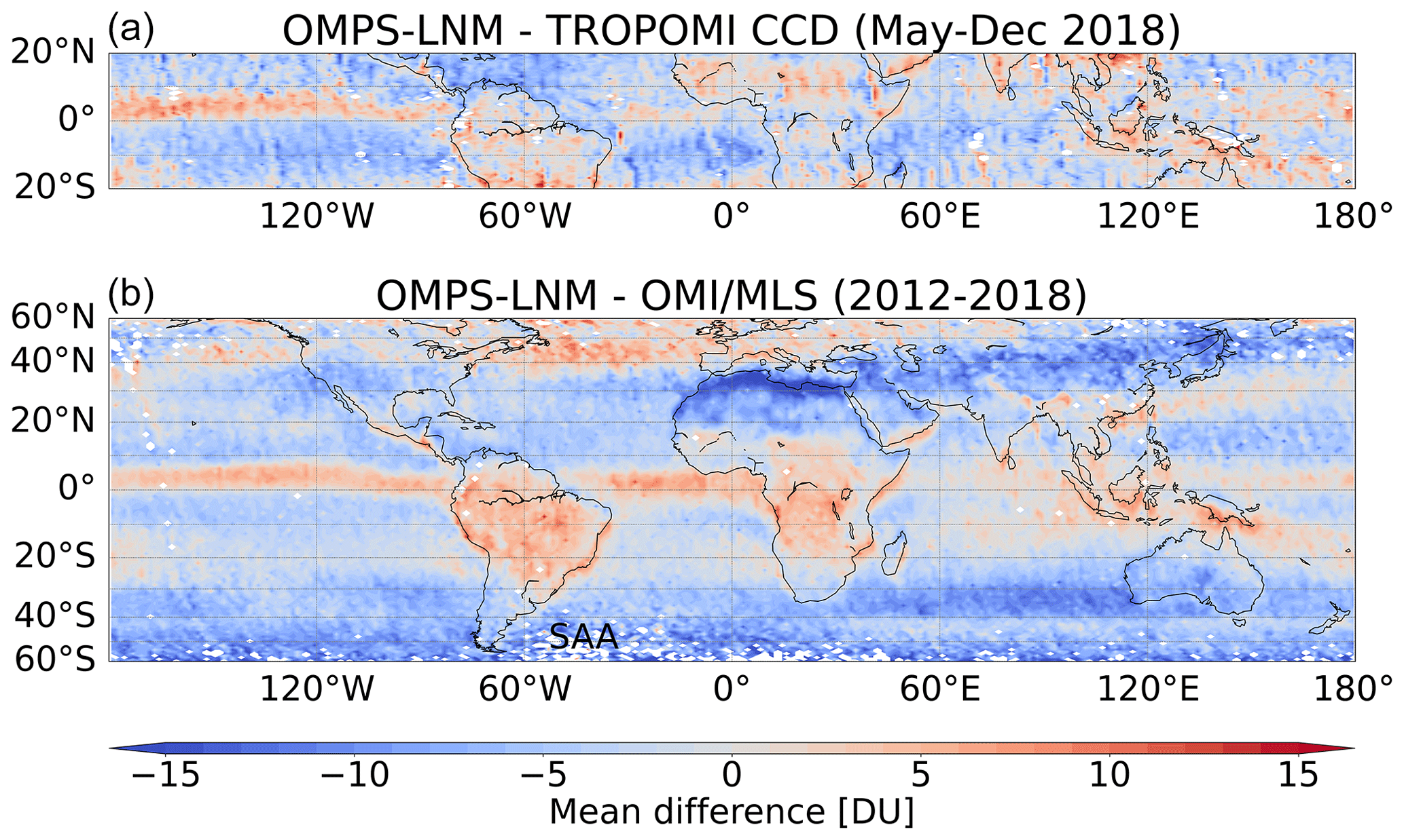
Figure 9 Mean differences in TrOC. (a) OMPS-LNM minus TROPOMI CCD from May to December 2018. (b) OMPS-LNM minus OMI/MLS from 2012 to 2018.

Both comparisons show similar patterns. Positive biases are observed in South America, central Africa, and the Indonesian region. Over the oceans, the differences are mostly negative, between 0 and 10 DU. As discussed above, the band of positive bias is observed between 0 and 10° N over the Pacific and Atlantic oceans. The bias over the Pacific Ocean ranges from 5 to 10 DU, while over the Atlantic, it is below 5 DU. In comparison with OMI/MLS, larger negative differences are observed in the southern extratropics that might result from the differences in the TPH definition. Over the northern extratropics, OMI/MLS shows higher values over Asia and north Africa, while OMPS-LNM is higher over the Atlantic Ocean. Higher values for OMPS-LNM are also observed in South America, Africa, and the Indonesian region. No seasonal variation in the differences is observed (not shown here). The general patterns observed in this comparison are similar to those seen in comparing the SOC from OMPS-LP and MLS (Fig. 7), indicating that the differences in TrOC are more influenced by the SOC.

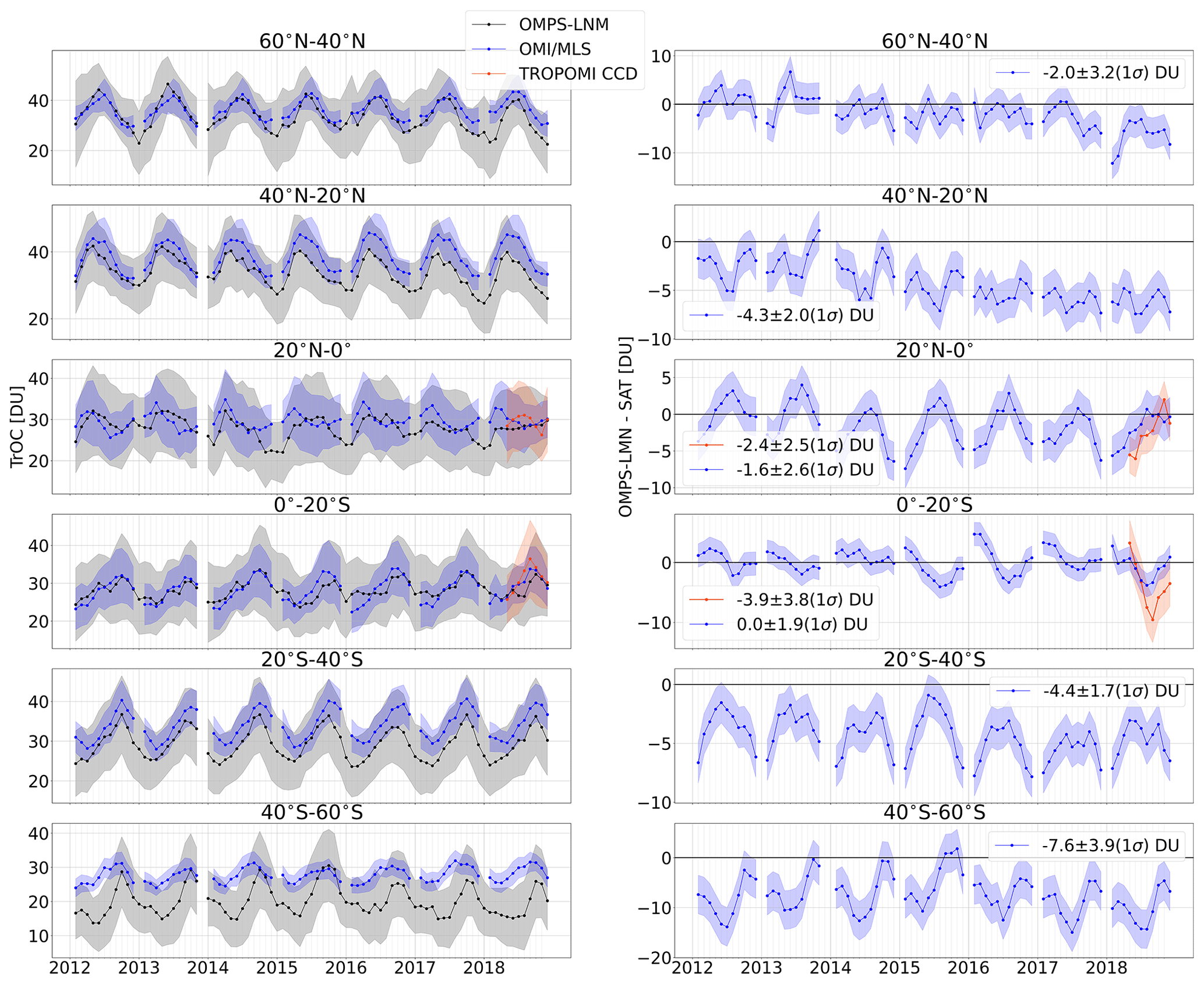
Figure 10 Zonal mean time series of TrOC from OMPS-LNM, OMI/MLS TOR, and TROPOMI CCD (left) and differences between the OMPS-LNM and other datasets (right) for six zonal bands. The shadings indicate the standard deviations of TrOC and of the differences.

Figure 10 shows monthly mean time series of TrOC (left panels) from OMPS-LNM (black), OMI/MLS (blue), and TROPOMI CCD (salmon) for six different zonal bands and differences between the OMPS-LNM and other datasets (right panels) from 2012 to 2018. Zonal bands from top to bottom are 40–60° N, 20–40° N, 0–20° N, 0–20° S, 20–40° S, and 40–60° S. Shadings mark the standard deviations of the averages and of the differences. In general, OMPS-LNM is lower than the other data, and the standard deviation of OMPS-LNM is higher than that of OMI/MLS. Very good agreement in the seasonal variation is observed, especially for the northern extratropics. In this latitude range, the mean difference between the OMPS-LNM and OMI/MLS is −2.0 ± 3.2 DU for the 40–60° N band and −4.3 ± 2 DU for 20–40° N. In the tropics, between the Equator and 20° N, no clear seasonality is observed for OMI/MLS. OMPS-LNM shows lower values during boreal winter, particularly low in 2015, 2016, and 2018. The TROPOMI CCD does not agree with the other two datasets in the northern tropical band. The mean bias of OMPS-LNM in this band is −1.6 ± 2.6 DU with respect to OMI/MLS and −2.4 ± 2.5 DU with respect to TROPOMI CCD. From 20° S to the Equator, OMI/MLS and OMPS-LNM agree with zero bias on average but show a difference of up to 5 DU in 2015 and 2016. In this region, the seasonal variability of TROPOMI CCD agrees with the other two datasets but shows a bias of −3.9 ± 3.8 DU with respect to OMPS-LNM. From 20 to 40° S, the seasonality of OMI/MLS data is similar to that of OMPS-LNM, and the mean bias between the datasets is −4.4 ± 1.7 DU. In the 40–60° S band, the mean difference between the datasets reaches −7.6 ± 3.9 DU. OMI/MLS shows a much weaker seasonality in this band. In contrast, OMPS-LNM shows more pronounced minima during austral autumn and maxima during austral spring. A drift is observed in the differences between OMI/MLS and OMPS-LNM, stronger for mid-latitudes and in the Northern Hemisphere. According to Jerry Ziemke (personal communication, 2024​​​​​​​), the OMI/MLS dataset needs to be corrected by −1.6 DU per decade. This correction would reduce the observed drift of about 5 DU for the analysed period between the datasets but not fully eliminate it. OMPS-LNM shows no drift in the ozonesonde comparison (Orfanoz-Cheuquelaf, 2023, pp. 91–92).

6 Summary and conclusions

This study presents a scientific tropospheric ozone column (TrOC) dataset from Suomi NPP OMPS-NM/OMPS-LP observations employing the limb–nadir matching (LNM) technique from 2012 to 2018. The data used in the retrieval, the retrieval approach, and the validation results of the OMPS-LNM TrOC dataset are discussed. A detailed analysis of the uncertainties of the underlying primary data, total ozone column (TOC), tropopause height (TPH) and stratospheric ozone column (SOC) is performed, and the overall uncertainty of the final TrOC product is estimated. Systematic and random components of the uncertainty are reported. The overall systematic TrOC uncertainty is estimated to be about 6.5 DU, and the overall random uncertainty is 12 DU for a single observation.

The OMPS-LNM TrOC data were validated using ozonesonde measurements and two TrOC satellite datasets, TROPOMI CCD (Hubert et al., 2021) and OMI/MLS TOR (Ziemke et al., 2006). The comparison with measurements from 22 ozonesondes sites shows a mean bias of $-\mathrm{1.7}\pm \mathrm{2.8}$ DU, with an average standard deviation of 9.9 DU. Half of the analysed sites show biases within 2 DU. We find a consistently negative bias when comparing OMPS-LNM TrOC with the two other satellite datasets. The mean bias between OMPS-LNM and OMI/MLS is $-\mathrm{3.4}\pm \mathrm{4.7}$ DU, with seasonal differences of up to 10 DU in the extratropics. Nevertheless, a good agreement in the long-term variability is observed. The mean bias between OMPS-LNM and TROPOMI CCD is $-\mathrm{1.8}\pm \mathrm{4.2}$ DU.

A retrieval artefact is identified over the Pacific and Atlantic oceans, showing a band of TrOC values increased by about 10 DU between the Equator and 10° N. The source for this anomaly is believed to be the impact of the gradient in the reflectivity along the instrument line of sight (LOS) on the retrieval of ozone profiles from limb-scatter measurements (OMPS-LP). The reflectivity gradient is related to a persistent belt of high clouds in the ITCZ region.

The OMPS-LNM TrOC dataset is considered to be suitable for analysing the spatial and temporal variability of tropospheric ozone and evaluating atmospheric models. It is important to consider the ITCZ's effect on the retrieval results and that the global OMPS-LNM data are, on average, 1 to 4 DU lower than other datasets considered here. This bias is, however, well within the estimated systematic uncertainty of OMPS-LNM TrOC. A new version of IUP OMPS-LP profiles is being processed based on the improved L1 (V2.6) data that counts for the observed drift after 2018. Using the improved stratospheric data, the OMPS-LNM TrOC dataset will be reprocessed and extended to the present and will be subject of a later paper.

Appendix A: Uncertainties in percentage

Table A1 Final uncertainty values in percentage for three typical TrOC values.