the Creative Commons Attribution 4.0 License.
the Creative Commons Attribution 4.0 License.
 | 15 Jan 2024
Research of low-cost air quality monitoring models with different machine learning algorithms
Gang Wang
Chunlai Yu
Kai Guo
Haisong Guo
Yibo Wang
To improve the performance of the calibration model for the air quality monitoring, a low-cost multi-parameter air quality monitoring system (LCS) based on different machine learning algorithms is proposed. The LCS can measure particulate matter (PM2.5 and PM10) and gas pollutants (SO2, NO2, CO and O3) simultaneously. The multi-input multi-output (MIMO) prediction model is developed based on the original signals of the sensors, ambient temperature (T) and relative humidity (RH), and the measurements of the reference instrumentations. The performance of the different algorithms (RF, MLR, KNN, BP, GA–BP) with parameters such as determination coefficient R2, root mean square error (RMSE), and mean absolute error (MAE) are compared and discussed. Using these methods, the R2 of the algorithms (RF, MLR, KNN, BP, GA–BP) for the PM is in the range 0.68–0.99; the RMSE values of PM2.5 and PM10 are within 2.36–18.68 and 4.55–45.05 µg m−3, respectively; the MAE values of PM2.5 and PM10 are within 1.44–12.80 and 3.21–23.20 µg m−3, respectively. The R2 of the algorithms (RF, MLR, KNN, BP, GA–BP) for the gas pollutants (O3, CO and NO2) is within 0.70–0.99; the RMSE values for these pollutants are 4.05–17.79 µg m−3, 0.02–0.18 mg m−3, 2.88–14.54 µg m−3, respectively; the MAE values for these pollutants are 2.76–13.46 µg m−3, 0.02–0.19 mg m−3, 1.84–11.08 µg m−3, respectively. The R2 of the algorithms (RF, KNN, BP, GA–BP, except for MLR) for SO2 is within 0.27–0.97, the RMSE value is in the range 0.64–5.37 µg m−3, and the MAE value is in the range 0.39–4.24 µg m−3. These measurements are consistent with the national environmental protection standard requirement of China, and the LCS based on the machine learning algorithms can be used to predict the concentrations of PM and gas pollution.
- Article
(8346 KB) - Full-text XML
- BibTeX
- EndNote


The development along with increased population and urbanization brings disadvantages, such as decreasing air quality and impact on public and individual health (Khreis et al., 2022; Manisalidis et al., 2020; Singh et al., 2021). Among the atmospheric pollutants, the primary pollutant is fine particulate matter, which affects the respiratory system and cardiac activity of humans. The secondary pollutants are SO2, CO, NOx, and O3, which also induce disease or chronic poisoning. To improve the understanding of air pollution exposure and predict future air quality trends (Zimmerman et al., 2018), air quality assessment and forecasting are the essentials. The conventional air quality monitoring instrumentations are high cost, which has limited the spatial coverage of the monitoring stations (Zimmerman et al., 2018). The development and applications of the low-cost commercially available sensor-based air quality monitoring system (LCS) would considerably reduce both installation and maintenance costs (Spinelle et al., 2017). The larger spatial density of the air quality grid monitoring network becomes possible, which would play an important role in monitoring pollution trends, locating pollution sources, supporting environmental management (Zhao et al., 2019), and supporting better epidemiological models (Khreis et al., 2022; Zimmerman et al., 2018). These demands promote the LCS growing gradually (Cui et al., 2021; Wang et al., 2016).
The LCS typically utilizes the electrochemical or light-scattering sensors for gas-phase or particulate pollutants measurement, such as sulfur dioxide (SO2), nitrogen oxide (NO2), carbon monoxide (CO), ozone (O3), and particulate matter (PM). These electrochemical sensors have intrinsic problems, such as temperature or humidity impacts, and gaseous cross-sensitivities (Spinelle et al., 2015, 2017; Jiao et al., 2016; Zimmerman et al., 2018). For example, limited by the poor selection performance, the NO2 electrochemical sensor also undergoes redox reactions in the presence of O3 gaseous pollutants. The diffusion coefficient of the electrochemical sensor can be affected by temperature and relative humidity (Hitchman et al., 1997; Masson et al., 2015). The reagent of the electrochemical sensor is consumed over time, which affects the stability of the sensor. These features of the sensors have historically been poorly addressed by laboratory calibrations, limiting the utility for air quality monitoring (Zimmerman et al., 2018).
The de-convolving of cross-sensitivity effect and stability on sensor performance is complex (Zimmerman et al., 2018). The linear or multivariate linear calibration models (Alexopoulos, 2010; Khreis et al., 2022; Zoest et al., 2019) have been developed. However the performance is poor in ambient data (Khreis et al., 2022). The accurate and precise calibration models for the low-cost sensors are particularly critical to the success of dense sensor networks, as poor signal-to-noise ratios and cross-sensitivities hamper their ability to distinguish the pollutant concentrations. There has been increasing interest in multifarious algorithms for low-cost sensor calibration, and lots of studies using multi-input multi-output models (Alexopoulos, 2010) and neural networks (Spinelle et al., 2015) have been published. The artificial neural network (ANN) calibration model has the intelligence to process nonlinear data (Amuthadevi et al., 2021; Janabi et al., 2021), which has been used in calibration models for measuring ozone or nitrogen oxide (Esposito et al., 2016; Spinelle et al., 2015). For example, the ANN calibration model was used to calibrate O3, and the uncertainty could meet the European data quality objectives; however, meeting these objectives for NO2 remained a challenge (Spinelle et al., 2015). Dynamic neural network calibrations of NO2 sensors were demonstrated with the mean absolute error less than 2 ppb; however, the performance for O3 was not the same (Esposito et al., 2016). High-dimensional multi-response model was used to calibrate CO, NO, NO2, and O3, with the 5 min average RMSE values of 39.2, 4.52, 4.56, and 9.71, respectively (Cross et al., 2017). A random-forest-based machine learning algorithm was used to improve the calibration strategies of low-cost sensors, with the mean absolute error values 38 ppb for CO, 10 ppm for CO2, 3.5 ppb for NO2, and 3.4 ppb for O3, respectively (Zimmerman et al., 2018). Furthermore, multiple-linear-regression-based (Ionascu et al., 2021) temperature and humidity correction and ANN-based calibration have shown potential for significant further improvement for leave-one-out cross-validation (Ali et al., 2021). With the 16 d process, the combined supervision calibration model was used to improve the R2 of SO2, NO2, and O3 by 75.8 %, 38.6 %, and 4.7 % to 0.58, 0.61, and 0.90, respectively (Cui et al., 2021). An integrated genetic programming dynamic neural network model was used to accurately estimate the carbon monoxide and nitrogen dioxide pollutant concentrations from the multi-sensor measurement data (Ari and Alagoz, 2022). A predictive model using multilayer perceptron, support vector regression, and linear regression was developed to analyze the CO2 and in-vehicle particulate matter, with the R2 of 0.9981 (Goh et al., 2021). The convolutional neural network (CNN), long–short-term-memory–convolutional-neural-network (LSTM-CNN), and CNN-LSTM models were used to improve the prediction performance of the ozone by 3.58 %, 1.68 %, and 3.37 %, respectively (Rezaei et al., 2023). However, these calibrations have only been tested utilizing fewer models with a short measurement period and small number of sensor matrices, each containing one sensor per pollutant (Cross et al., 2017; Esposito et al., 2016; Spinelle et al., 2015); they have not been utilized to evaluate and predict the concentration values of multi-pollutants simultaneously, such as PM2.5, PM10, SO2, NO2, CO, and O3.
The random forest (RF) (Breiman, 2001; Liu et al., 2012), multivariate linear regression (MLR) (Alexopoulos, 2010), K-nearest neighbor (KNN) (Zhao and Lai, 2021), back propagation (BP) neural network (Xu et al., 2021), and genetic-algorithm–back-propagation neural (GA–BP) network (Ning et al., 2019; Wang et al., 2019) are five commonly used machine learning algorithms with different characteristics. With the strong nonlinear mapping ability and adaptive ability, the RF, BP, and GA–BP are suitable for processing complex, high-dimensional, and nonlinear data with high prediction accuracy, such as the air quality monitoring. With the purpose of quantifying the degree of influence of the independent variable, the MLR is suitable for evaluating the influence of multiple independent variables on the dependent variable, such as the cross-sensitivity effect between different factors. The KNN is also a widely common algorithm to compare with RF, BP, GA–BP, and MLR.
In this work, the LCS is developed to measure PM2.5, PM10, SO2, NO2, CO, and O3 simultaneously, and the performances of the calibration strategies based on the five machine learning algorithms are contrasted. Taking the original electronic signals of the sensors as input and measurements obtained by the reference instrumentations as output, five calibration strategies are applied and contrasted. The measurement is implemented under real-world conditions within almost a 12-month period (1 March 2021 and 28 February 2022) spanning multiple seasons and a wide range of meteorological conditions to ensure calibration model robustness. The performance of the different algorithms with the parameters, such as determination coefficient (R2), root mean square error (RMSE) (Janabi et al., 2021), and mean absolute error (MAE), is compared and discussed. The rest of this paper is organized as follows. The measurement setup is described in Sect. 2. The principles of the calibration strategies are presented in Sect. 3. The results and discussion are shown in Sect. 4. The conclusion and discussion are drawn in Sect. 5.
This section describes the measurement site and data collection, schematic block of the LCS, and the reference instrumentation. The low-cost here is defined as below USD 150 per pollutant, commercial availability, and low maintenance. The sensors typically utilize electro-chemical signal and scattering light intensity for gas-phase pollutant (SO2, NO2, CO and O3) and particle pollutant (PM2.5, PM10) measurements.
2.1 Measurement site and data collection
Measurements for gas-phase pollutants and particle pollutants were made continuously between 1 March 2021 and 28 February 2022, which were used as the start and end dates for the analyses. The location, shown in Fig. 1, was 30 Yaochang Street, Zhongyuan District, Zhengzhou, Henan Province of China. There was an independent reference monitoring system for PM2.5, PM10, CO, SO2, NO2, and O3 measurement. The LCS was mounted at a consistent height with the reference monitoring system. The time taken for one set of data collection was 1 min and repeated four times. The outlier of the four sets of data was eliminated by using the Dixon principle. The remaining data were used to get the mean values for each experiment. The values of the LCS and reference instruments were separately logged to the server with an interval of 5 min. During the measurement period, the ranges of the ambient temperature and relative humidity separately were −5 to +50∘C and 10 % to 98 %.
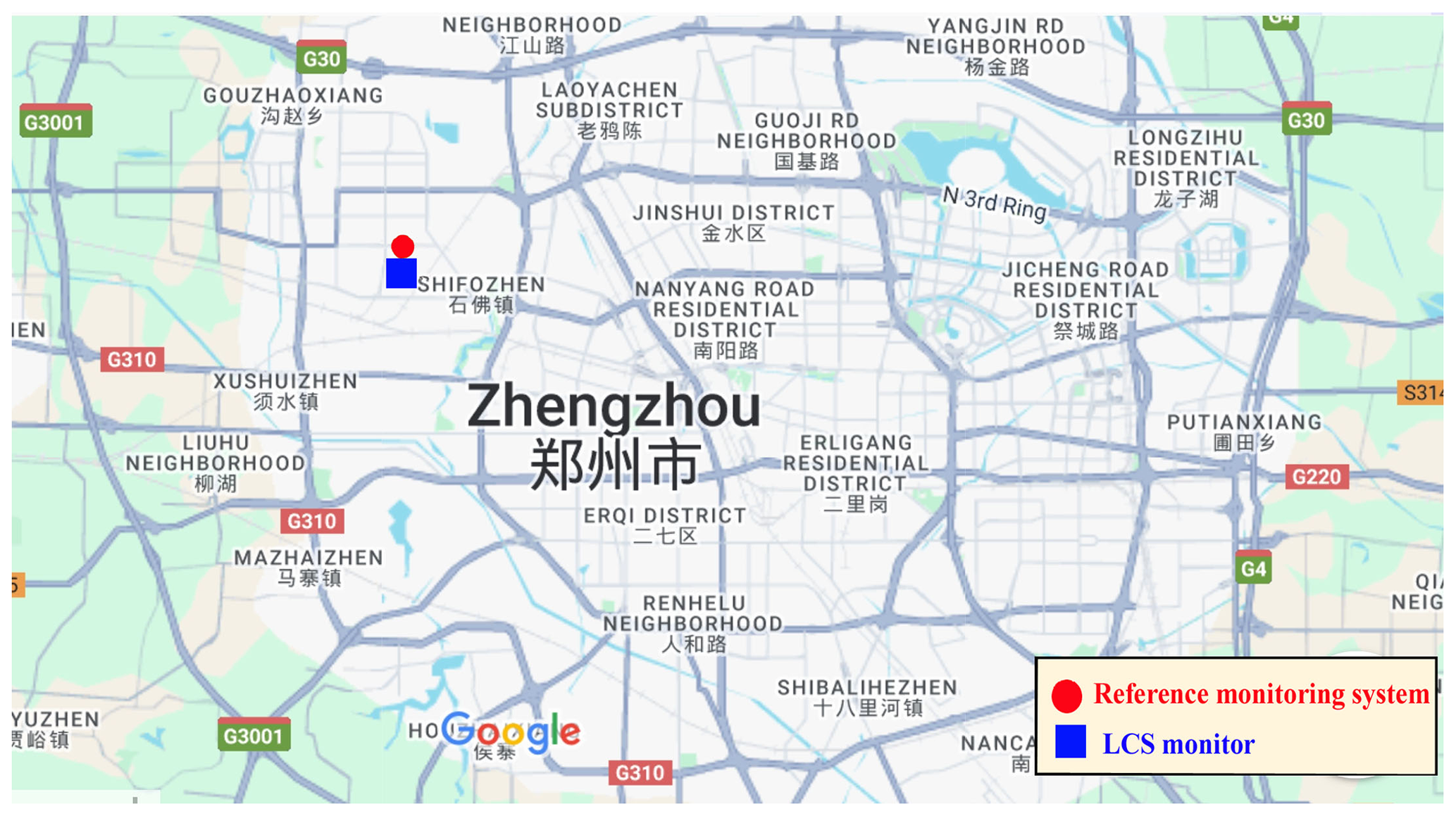
Figure 1Location of the air quality monitoring station during the measurement period.
2.2 Schematic block of LCS
In this study, the LCS is developed by Hanwei Electronics Group Corporation, and its schematic block diagram is shown in Fig. 2. The LCS uses a commercially available particulate matter sensor (PM3006, Cubic sensor and Instrument Co., China) and electrochemical SO2, NO2, O3, and CO sensors (B4, Alphasense, UK), respectively. The particulate matter sensor device is a laser-diode (LD)-based particle sensor, using a spectrophotometer to measure the particle scattering light intensity. The PM sensor device (PM3006) can measure size-dependent PM2.5 and PM10 concentration of the particles in the size range of 0.3 to 10 µm. The gas pollution (SO2/NO2/O3/CO) sensors used are with four electrodes (i.e., reference, worker, counter, and auxiliary electrodes), where the auxiliary electrode is not exposed to the target analyte to account for changes in the sensor baseline signal under different meteorological conditions (Mead et al., 2013).
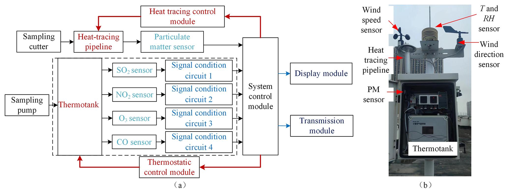
Figure 2Schematic block and site photo of the LCS. Panel (a) is the schematic block of the LCS. The system control module can ensure the temperature stability of the heat tracing pipeline and thermo-tank through the heat tracing control module and thermostatic control module, respectively. The sampling cutter is used to filter particles larger than 10 µm. The sampling pump is utilized to deliver ambient air to the surface of the sensors. Panel (b) is the site photo of the LCS.
The electrochemical sensor outputs are measured using electronic circuitry designed by Hanwei and optimized for signal stability. The circuitry is developed with custom electronics to drive the device, multiple stages of filtering circuitry for specific noise signatures, and an analog-to-digital converter for measurement of the conditioned signal.
Due to the redox reaction on the anode and the cathode of the electrochemical sensor, the movement of charge between the electrodes produces a current proportional to the analyte reaction rate, which can be used to determine the analyte concentration (Mead et al., 2013) and whether the sensor is working effectively.
Before installed into the LCS, calibrated with the different models and used in real-world conditions, the performance of the sensors should be checked in the laboratory. The linearity of the gas sensors was tested under steadily increased concentration, which was from 0–5 mg m−3 for CO sensor, 0–0.2 mg m−3 for NO2, 0–1.1 mg m−3 for O3, and 0–1.4 mg m−3 for SO2 with five more test points, shown in Fig. 3. Since the units of outputs of the reference instruments and the sensors were different, the slope was not expected to be 1 (Cui et al., 2021). As shown in Fig. 3, the R2 for the gas sensors is more than 0.93, which indicated that these gas sensors have good linear responses before calibration and verified the sensor is working properly and effectively and could be applied to the LCS.
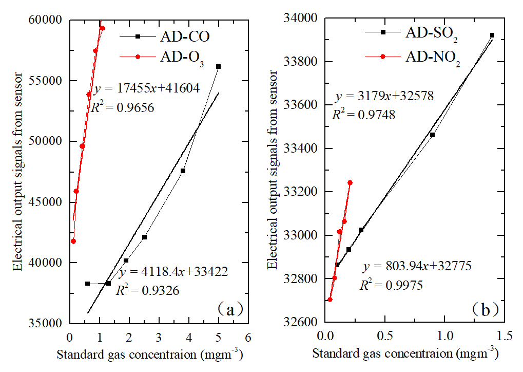
Figure 3Linearity of gas sensors before calibration. Electrical output signals versus single standard gas concentration is tested in laboratory conditions. Panels (a) and (b) represent the proportional relations between CO and O3 sensors as well as SO2 and NO2 sensors, respectively. The duration of each measurement is about 30 min.
However, even with an auxiliary electrode, electrochemical sensors may insufficiently account for the impacts of temperature and relative humidity. With the standard gases through the test chamber and the concentrations stabilized at 27 ppb for SO2, 3.9 ppb for NO2, 13 ppb for O3, and 1.22 ppm for CO, the output voltages of the four types of gaseous sensors are nonlinearly fluctuated with the linearly increasing temperature and the relative humidity (RH) (Cui et al., 2021). With the purpose of eliminating the influence of the external environment on the sensor as much as possible, the particles flow through a sampling cutter and heat-tracing pipeline to the particulate matter sensor, and the gaseous pollutants are pumped to the electrochemical sensors, which are secured in a thermo-tank. The temperature values of the heat-tracing pipeline and thermo-tank can be maintained at 60∘ ± 2∘C to reduce the influence of relative humidity and 25∘ ± 2∘C (Wei et al., 2018) to keep the sensor operating at a stable temperature, respectively.
The measurement results of particulate matter sensor and gas pollution sensors, transmitted to the system control module through the data buses, are directly displayed on the local display module and wirelessly transmitted to the corresponding online server through the transmission module. As the uni-variate linear models do not incorporate any cross-sensitivities to other pollutants or any nonlinearities in the response, we attempt to use the sensor electronic results as the input and the reference measurements as the output, to build multi-dimensional multi-response prediction models to de-convolve the effects of cross-sensitivity and stability on sensor performance utilizing MLR, RF, KNN, BP, and GA–BP calibration models.
2.3 Reference instrumentation
In order to reduce the adsorption effect on particle matter and gaseous pollutants, the reference measurements are made on ambient air continuously drawn through Teflon fluorinated ethylene propylene (FEP) (Wei et al., 2018) tubing with a six-port stainless-steel manifold for flow distribution to the gas analyzers and particulate monitors (Mead et al., 2013). It should be pointed out that the LCS was mounted at a consistent height with the reference monitoring system during the measurement period.
The reference ambient particulate monitor 5014i, which uses beta attenuation of the ambient particulate deposited onto a filter tape, is applied to measure the mass concentration of suspended and refined particulates. The reference NO–NO2–NOX monitor 42i, using the linear proportional of the chemi-luminescence reaction of NO and O3 after NO2 transformed into NO, is utilized to measure the NO2 concentration. The SO2 reference analyzer is 43i using the ultraviolet light (which is emitted as the excited SO2 molecules decay to lower energy states) intensity proportional to the SO2 concentration. The CO reference monitor is 48i utilizing the principle that CO absorbs infrared radiation at a wavelength of 4.6 µm, and the infrared absorption can be transformed to be proportional to the CO concentration. The 49i O3 analyzer operates on the principle that O3 molecules absorb UV light at a wavelength of 254 nm, and the absorption intensity of the UV light is directly related to the ozone concentration. All these reference monitors are produced by Thermo Fisher Scientific Inc. The time interval for all reference measurements is 5 min. According to the technical specifications for operation and quality control of ambient air quality of the continuous automated monitoring system for SO2, NO2, O3 ,and CO of China (Ministry of Ecology and Environment of the People's Republic of China, 2018), as well as the technical guide for automatic monitoring by beta ray method for particulate matter in ambient air (PM10 and PM2.5) (Ministry of Ecology and Environment of the People's Republic of China, 2020), the reference gas and particulate analyzers are checked and calibrated weekly and monthly, respectively.
This section describes the principles of the calibration methods, such as MLR, BP, GA–BP, KNN, and RF and the metrics for performance evaluation. The calibration models are constructed with the sensors' (i.e., PM2.5, PM10, CO, SO2, NO2, and O3 sensors) electronic results as the input and the reference measurements as the output.
3.1 Calibration methods
3.1.1 Multiple linear regression model
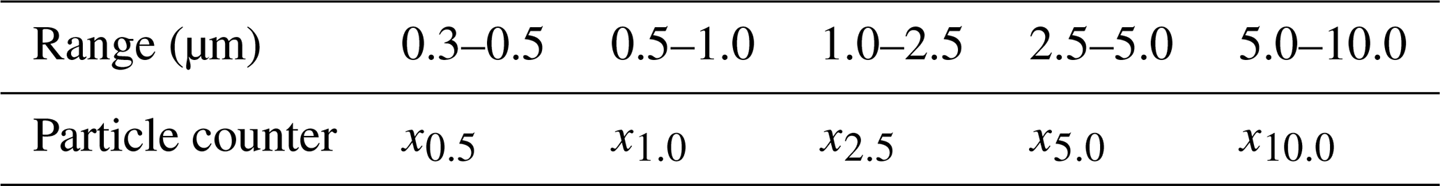
After the data collected by the LCS, the raw data should be preprocessed. The PM3006 particulate matter sensor can output six kinds of particle range (i.e., > 0.3, > 0.5, > 1.0, > 2.5, > 5.0 and > 10 µm, respectively). By subtracting the six particle range values in turn, the individual particle counters are obtained and expressed as x0.5, x1.0, x2.5, x5.0, and x10.0 (listed in Table 1). The measured particle number concentration is converted to PM mass concentrations in the PM2.5 and PM10 size fractions.
Table 1Size range of the particulate matter sensor. The sensor can measure particles with the size range of 0.3–0.5, 0.5–1.0, 1.0–2.5, 2.5–5.0, and 5.0–10 µm, simultaneously. The corresponding particle counters are expressed as x0.5, x1.0, x2.5, x5.0, and x10.0, respectively.
Taking the particle counters, listed in Table 1, as input and the concentrations YPM2.5 and YPM10 of PM2.5 and PM10 measured by 5014i as output, the multivariate linear regression (MLR) models (Alexopoulos, 2010; Zoest et al., 2019) are built. Due to the previously established influence of ambient temperature (T) and relative humidity (RH) on sensor response (Masson et al., 2015; Jiao et al., 2016), the particle counter terms are pretreated and individual from each other. The multi-input one-response preprocessing and prediction models can be written as Eq. (1) to obtain the YPM2.5 concentrations.
where WPM2.5 = [w1_PM2.5, w2_PM2.5, w3_PM2.5, w4_PM2.5, w5_PM2.5] denotes the corresponding weight coefficients; the XPM2.5 = [x0.5, x1.0, x2.5, T, RH] represents the individual particle counters, the temperature sensor and humidity sensor; the bPM2.5 is the intercept value of the model.
To obtain the concentration YPM10, the multi-input one-response preprocessing and prediction models can be written as Eq. (2).
where WPM10 = [w1_PM10, w2_PM10, w3_PM10, w4_PM10, w5_PM10, w6_PM10, w7_PM10] denotes the corresponding weight coefficients; the XPM10 = [x0.5, x1.0, x2.5, x5.0, x10.0, T, RH] represents the individual particle counters, the temperature sensor and humidity sensor; the bPM10 is the intercept value of the model.
Due to the poor selection performance and cross interference of the electro-chemical sensor response, the output values from the sensors and the concentrations of the target pollutants, such as O3, NO2, and SO2 concentrations, measured by the inference monitor are used to build the MLR model. The CO gaseous pollution is also one of the criteria pollutants, which must be measured in China. Thus, the multi-dimensional multi-response preprocessing and prediction model for the four types of gas pollution, T, and RH can be written as Eq. (3).
Equation (3) can be simplified as
where
is the corresponding weight coefficient; the Xgas = [, , xCO, , T, RH] is the convertor output values of the sensors through the electronic circuitries; the Bgas = [, , bCO, ] is the intercept value of the model.
Hereto, the multi MLR models for the gas sensor and PM sensor are separately developed. The training data are used to calculate the model regression coefficient and intercept values, and the withheld testing data are utilized to evaluate the performance of the model performance.
3.1.2 BP neural network model
The BP neural network algorithm is one of the most widely used ANN models. It is a multi-layer feed-forward network trained through an error back propagation algorithm by constantly adjusting the weight and intercept of the network. The feed-forward topological structure of the BP neural network model, shown in Fig. 4, includes the input layer, hidden layer, and output layer. With the purpose of avoiding the numerical problems caused by the extreme values of polarization, eliminating the misleading effects for feature extraction, and obtaining the accurate estimation of pollutant concentrations (Janabi et al., 2021), the collected input sensor date XI and output date YO should be respectively normalized with min–max normalization to limit values in each dimension between 0 and 1 (Bakiler and Guney, 2021).
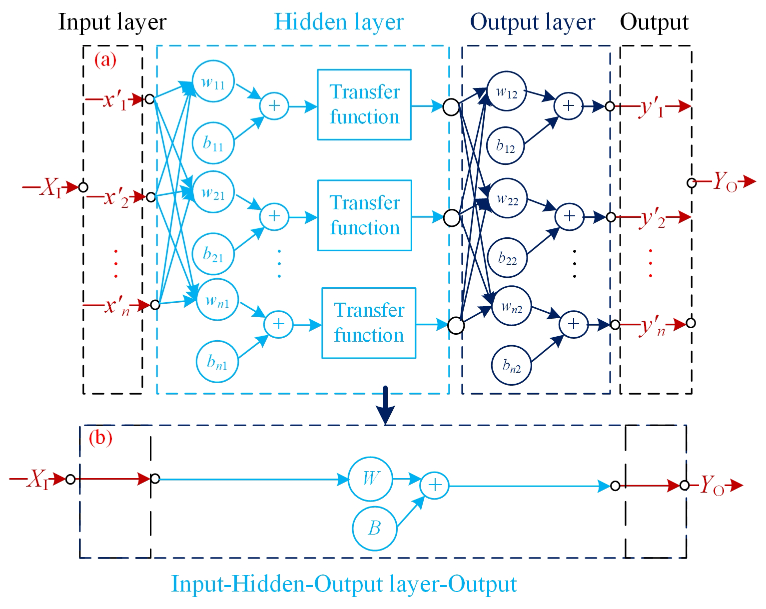
Figure 4Topological structure of BP neural network model. Panel (a) is the feed-forward topological structure. The XI and YO are the input data and output data, respectively. The and separately indicate the normalized items of X and Y. The wi1 and bi1 as well as wj2 and bj2 separately represent the weight value and intercept value of the hidden layer and output layer. Panel (b) is equivalent to panel (a) to simplify the formulas.
After the normalization process, the BP network can be established. To optimize the best parameters of the network, the number of hidden layers, the transfer functions of the layers, and the end conditions should be determined. If the parameters are inappropriate, the BP model will be overtrained or insufficient. In this study, a shallow structure with a single hidden layer is chosen, as extensive testing did not show any noticeable improvement in calibration performance with deeper structure consisting of multiple hidden layers (Ali et al., 2021). This also reduced the complexity and the training time.
3.1.3 Genetic algorithm–BP model
In the traditional BP neural network, the initial weights and thresholds are randomly generated. The results often fall into a local minimum rather than a global minimum and would lead to the distortion of the prediction result. In addition, the convergence speed of the BP neural network is usually slow. To solve these problems, the genetic algorithm (GA) (Liang et al., 2018) with BP algorithm is also used to avoid the inherent defects of BP algorithm. The GA method is essentially a direct search method that does not rely on specific problems and gradient information. It follows the survival and elimination rule of biological evolution, generates the following hypotheses by mutating and reconstructing the best existed hypothesis, and makes it possible to solve the problem (Ning et al., 2019). Generally, the GA is used to find an optimal initial weight and a threshold value for the model, so that the model could converge in the direction of a minimum value (Wang et al., 2019). The GA–BP hybrid algorithm is used to reduce the time for the BP neural network to adjust the weight and threshold itself and achieve the goal of improving work efficiency.
3.1.4 K-nearest neighbor model
The k-nearest neighbor (KNN) is also one of the simplest methods for classification as well as regression problems (Kumar, 2015; Zhao and Lai, 2021). The KNN is a supervised method that uses estimation based on values of neighbors, which can automatically adapt to the supervised learning problems with arbitrary Bayes decision boundaries (Zhao and Lai, 2021). From the supervisor data set, the KNN solution utilizes the values of given dependent variable yi to approximate the dependent variable y∗, which is close with respect to distance between their corresponding model parameters. For the regression problem, the mean of the observed labels of k-nearest neighbors of independent variable X is assigned to be the predicted label. In this study, the k is set to 10 with the performance having no obvious difference from other numbers.
3.1.5 Random forest model
The random forest (RF) model is used for solving regression or classification problems (Breiman, 2001; Liu et al., 2012). It works by constructing an ensemble of decision trees using a training data set; the mean value from that ensemble of decision trees is then used to predict the value for new input data (Zimmerman et al., 2018). With the purpose of establishing a RF model, the maximum number of decision trees of the forest should be specified. Each tree is constructed using a bootstrapped random sample from the training data set. By considering a random subset of the possible explanatory variables with the strongest predictor of the response, the origin node of the decision tree can be split into sub-nodes. The node-splitting process is repeated until a terminal node is reached. The terminal node can be specified using the maximum number of sub-nodes or the minimum number of data points in the node. To illustrate the method, consider building a random forest model for one LCS using a single decision tree and a subset of 20 490 data points to build a calibration model, shown in Fig. 5. The RF model can predict data with variable parameters within the training range. Therefore, a larger and more variable training data set should create a better final model. To avoid missing any spikes during the training window, a 5-fold cross-validation approach (Zimmerman et al., 2018) is also used to maximize utilization of the training data set. This approach helps to minimize bias in training data selection when predicting new data and ensures that every point in the training window is used to build the model.
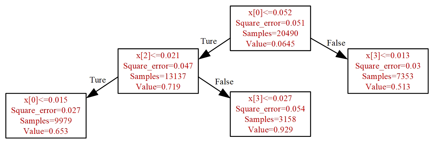
Figure 5Simplified illustration of the RF with a single decision tree and a subset. The x[0], x[2], and x[3] represent the CO, SO2, and O3 pollutants. At the first split, points with normalized CO sensor signal ≤ 0.052 are sent to a terminal node; the remaining points go to the other splitting node. The sample is the number of data points in each terminal node. The value is the average in each terminal node.
3.2 Metrics for performance evaluation
To quantitatively compare the performances of the five calibration models applied to the LCS, and balance the disadvantages of the different metrics, the determination coefficient (R2), root mean square error (RMSE) (Janabi et al., 2021), and mean absolute error (MAE) are utilized. The R2 reflects the fit degree between the model output data and the reference monitor measurement. The measurement results should meet the requirements of environmental standards of China (Jiao et al., 2016). The RMSE measures how much error there is between the predicted values and the reference measurements and is sensitive to extreme values (Chai and Draxler, 2014). The MAE is a good choice to evaluate the error when the distribution is not Gaussian (Rezaei et al., 2023). The formulas for the evaluation metrics are presented as Eqs. (5)–(7), respectively.
where , yi, and represent the ith model output data from the algorithm-based LCS system, the reference data from the reference instrumentations, and the mean value of the reference instrumentations, respectively. The n is the number of the measurement data in the data set.
Following the model building, the goodness of regression and root mean square error between the model output concentrations and the reference monitor concentrations are evaluated for all calibration model approaches. The plots for the PM2.5, PM10, O3, CO, NO2, and SO2 illustrating the time series and goodness of fit of the models are provided in Figs. 6–15. The R2 and RMSE values are listed in Tables 2–7.
4.1 Parameters of the model
For the BP and GA–BP models, the parameters are the functions for the hidden layer and output layer, the type of the hidden layer, the number of iteration times, and the number of the nerve units (Xu et al., 2021). The functions for the hidden layer and output layer in this study respectively are the default tansig and the purelin functions. With the more complex type of the hidden layer and less obvious improvement, the hidden layer is single type to achieve the goal of work efficiency.
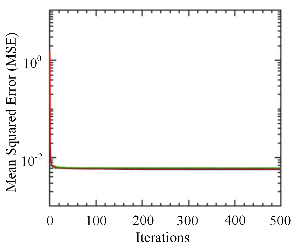
To determine the best number of iteration times and nerve units, the measurement from the LCS and reference monitor between 1 March and 30 June 2021 is used. The number of iteration time is optimized using the mean squared error (MSE) between the model value from the model and the reference monitor output value. The tendency of the MSE is shown in Fig. 6. The training is performed for 500 iterations. It is observed that the MSE decreases with the number of iterations increasing; the rate of decrease and the variation of the MSE is negligible beyond 100 iterations. More iterations incur higher computational cost for the training and small performance improvement. There is also the risk of overtraining resulting in poor generalization capability. Using this method, the same number of iterations can be obtained with the different gas pollutants within 1 July and 31 October 2021 as well as 1 November 2021 and 28 February 2022.
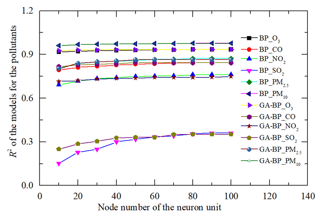
The node number of the nerve units is determined by the contrast results of determination coefficient R2 for different gas and PM pollutants within 1 March and 30 June 2021. The results are shown in Fig. 7. The R2 is improved as the number of nerve units increasing. The rate of increase and the variation of R2 is negligible beyond 70 units. More units incur higher computational cost and time for the training and small performance improvement. Using this method, the same number of the nerve units can be obtained with the different gas pollutants within 1 July and 31 October 2021 as well as 1 November 2021 and 28 February 2022.
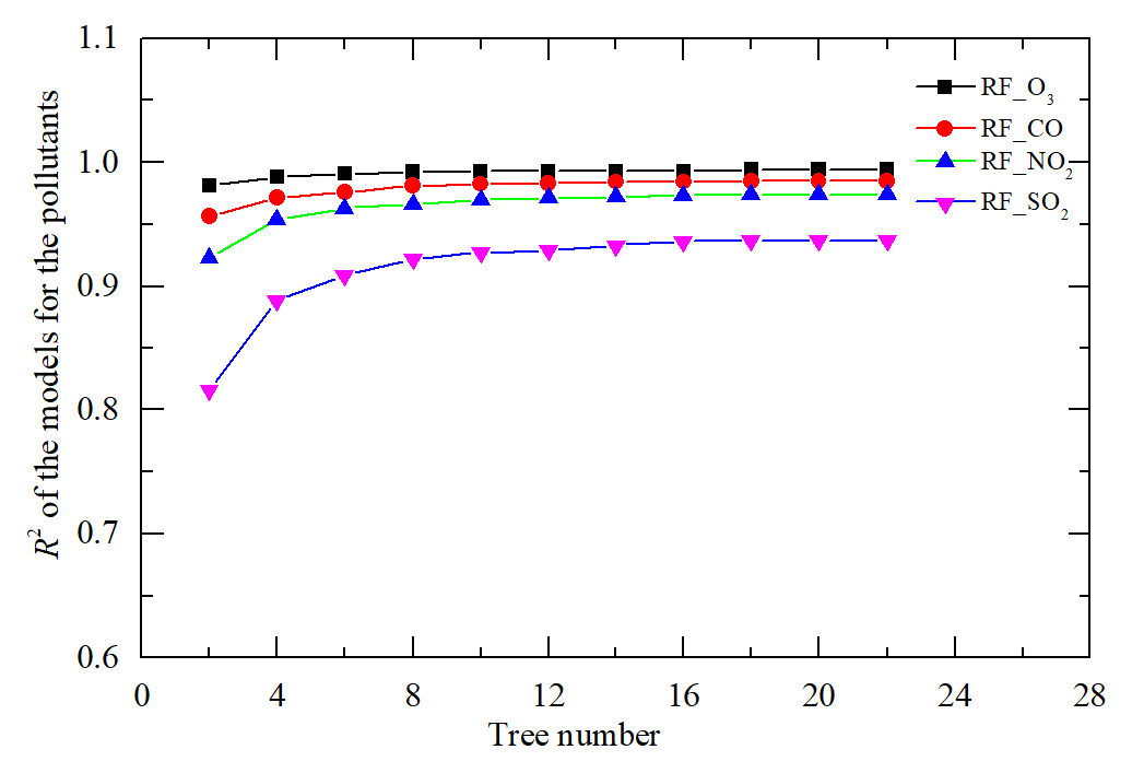
For the RF model, the number of trees is determined by using grid search method, which will search the optimal hyper-parameter by traversing a given hyper-parameter combination (Zhu et al., 2022). A total of 11 kinds of tree numbers are set between 2 and 22 by using grid search to traverse these 11 kinds of tree numbers to obtain different R2. For instance, the R2 values for different gas pollutants within 1 March and 30 June 2021 are shown in Fig. 8. The R2 is improved as the number of trees increases. The rate of increase and the variation of R2 is negligible beyond 20. The terminal node is specified using a maximum number of sub-node points per node. The R2 is also improved as the number of sub-nodes increases under the same tree number. The rate of increase and the variation of R2 is negligible beyond 100. A higher number of trees or sub-nodes incurs higher computational cost and time for the training and small performance improvement. Using this method, the same number of trees can be obtained with the different gas pollutants within 1 July and 31 October 2021 as well as 1 November 2021 and 28 February 2022.
4.2 Measurement results of PM
With the purpose of avoiding over-fit in the five models, the random partition parameters of train ratio and test ratio are 80 % and 20 %, respectively. To ensure the robustness of the model evaluation, the 5-fold cross validation is also conducted. The data set is divided into five mutually exclusive subsets with same size, where the four subsets are randomly selected as the training set each time, and the remaining subset is used as the test set. After completing each round of validation, four copies are selected again to train the model and the remaining copy is used for validation. After several rounds (less than five), the loss function is selected to evaluate the optimal model and parameters (Mahesh et al., 2023; Zimmerman et al., 2018).
With the results from 1 March 2021 to 28 February 2022 and according the trend of the ambient temperature, the total data are divided into three segments. The three segments (I, II, and III) separately are within 1 March and 30 June 2021 with the size of 32 481, 1 July and 31 October 2021 with the size of 31 287, and 1 November 2021 and 28 February 2022 with the size of 32 053, respectively.
During the measurement period, the ranges of the ambient temperature and relative humidity separately were −5 to +50∘C and 10 % to 98 %, shown in Fig. 9. The ambient temperature increased, decreased, and fluctuated separately within 1 March and 30 June 2021, 1 July and 31 October 2021, and 1 November 2021 and 28 February 2022. The time series data and regressions of five modes for PM from reference monitor and LCS calibration output are shown in Figs. 10 and 11.
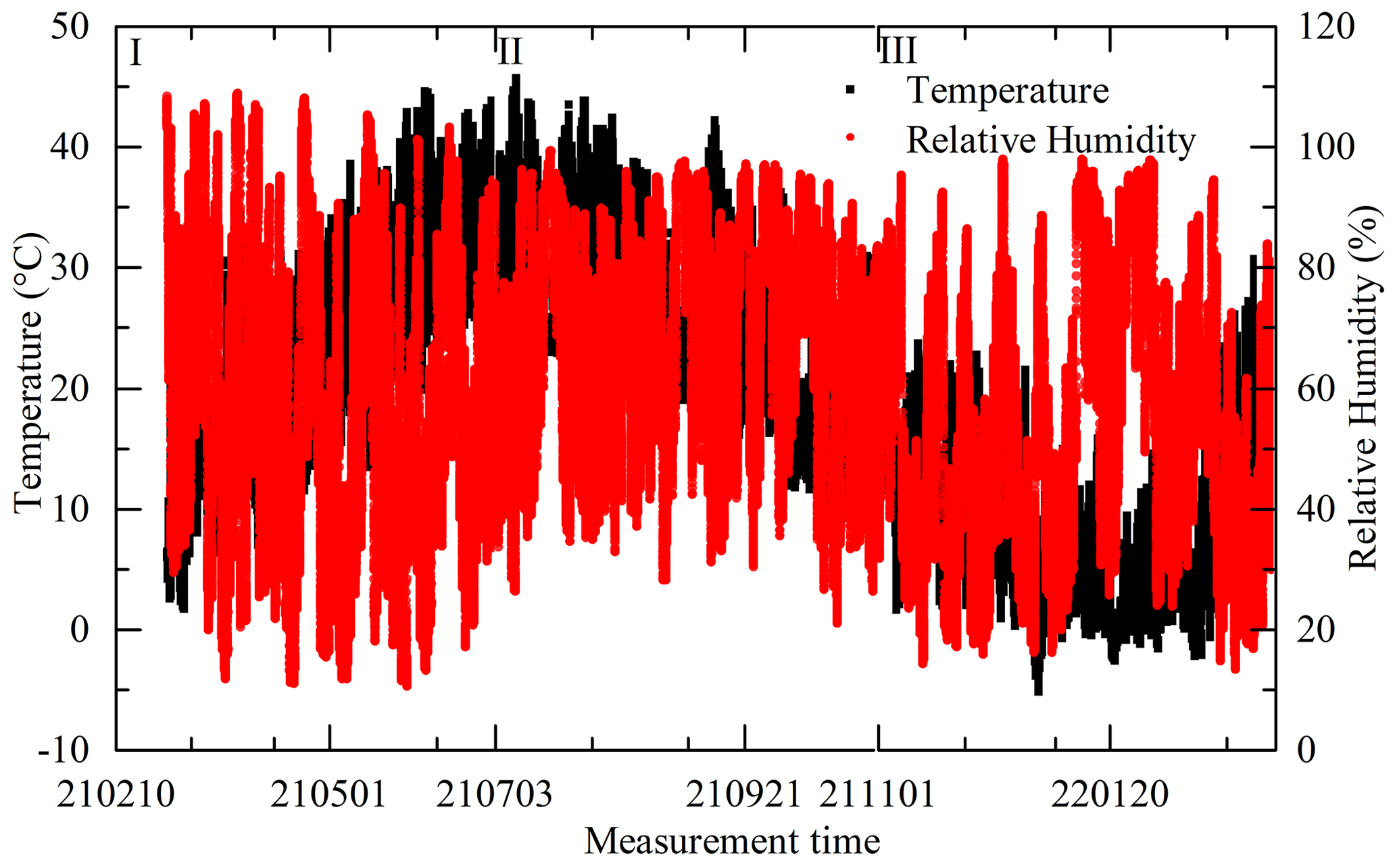
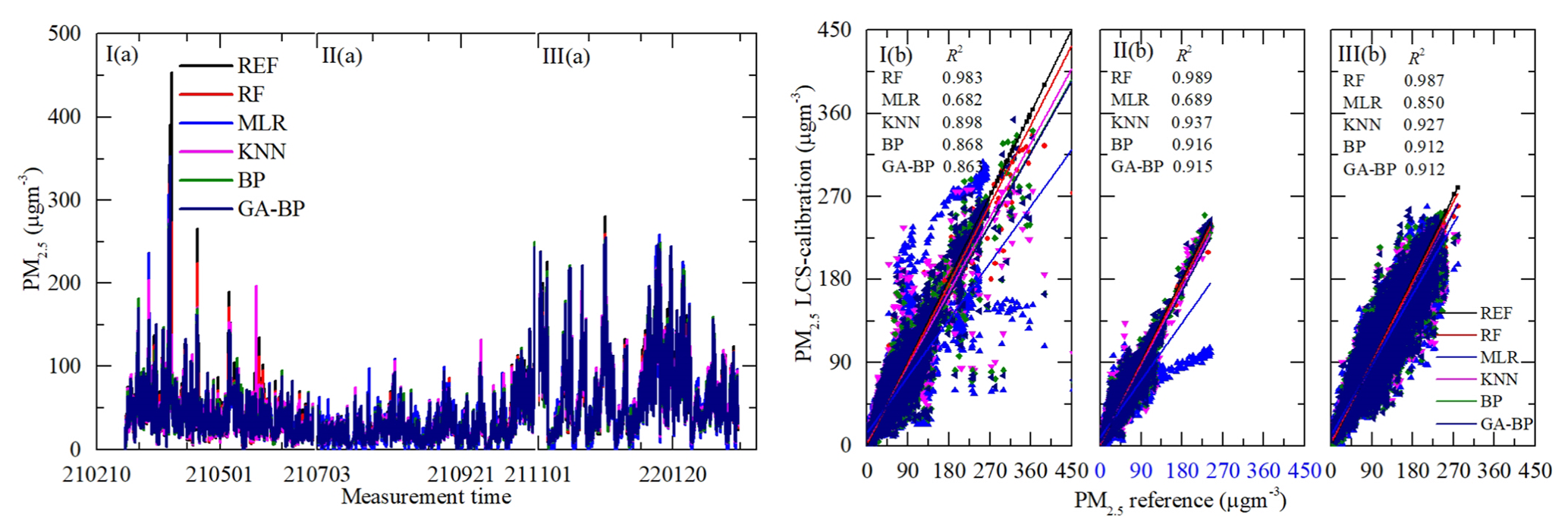
Figure 10Time series and regressions comparing the reference monitor PM2.5 data (black) to five calibration model PM2.5 results, where red, blue, magenta, olive, and navy represent RF, MLR, KNN, BP, and GA–BP, respectively. Panel (a) shows the whole time series data of the measurement period. Panel (b) shows the regressions of the five calibration models.
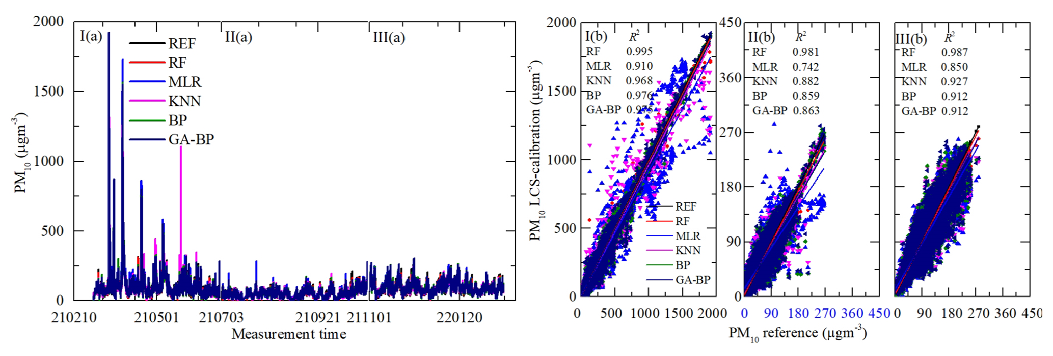
Figure 11Time series and regressions comparing the reference monitor PM10 data (black) to five calibration model PM10 results, where red, blue, magenta, olive, and navy represent RF, MLR, KNN, BP, and GA–BP, respectively. Panel (a) shows the whole time series data of the measurement period. Panel (b) shows the regressions of the five calibration models.
As shown in Figs. 10a and 11a, the general tendencies of the data fluctuation between the reference monitor and the RF, MLR, KNN, BP, and GA–BP algorithms of the LCS are consistent with each other. The RF model has the best performance, followed by KNN, BP, and GA–BP, with MLR having the worst.
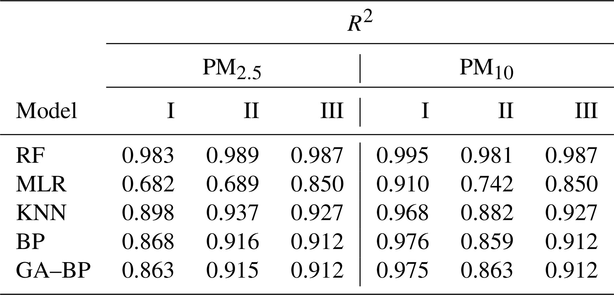
The R2 values between the reference data and the five model data are also shown in Figs. 10b and 11b and listed in Table 2. The R2 of RF for the PM is better than 0.98. The R2 of MLR for the PM is less than 0.91 and even less than 0.7. The R2 values of the other three models are within 0.86 and 0.98.
Table 2Performance of different calibration models for the PM2.5 and PM10 against the reference monitor. The determination coefficient R2 (higher is better, maximum of 1) of different calibration models (RF, MLR, KNN, BP, GA–BP) versus the reference monitor.
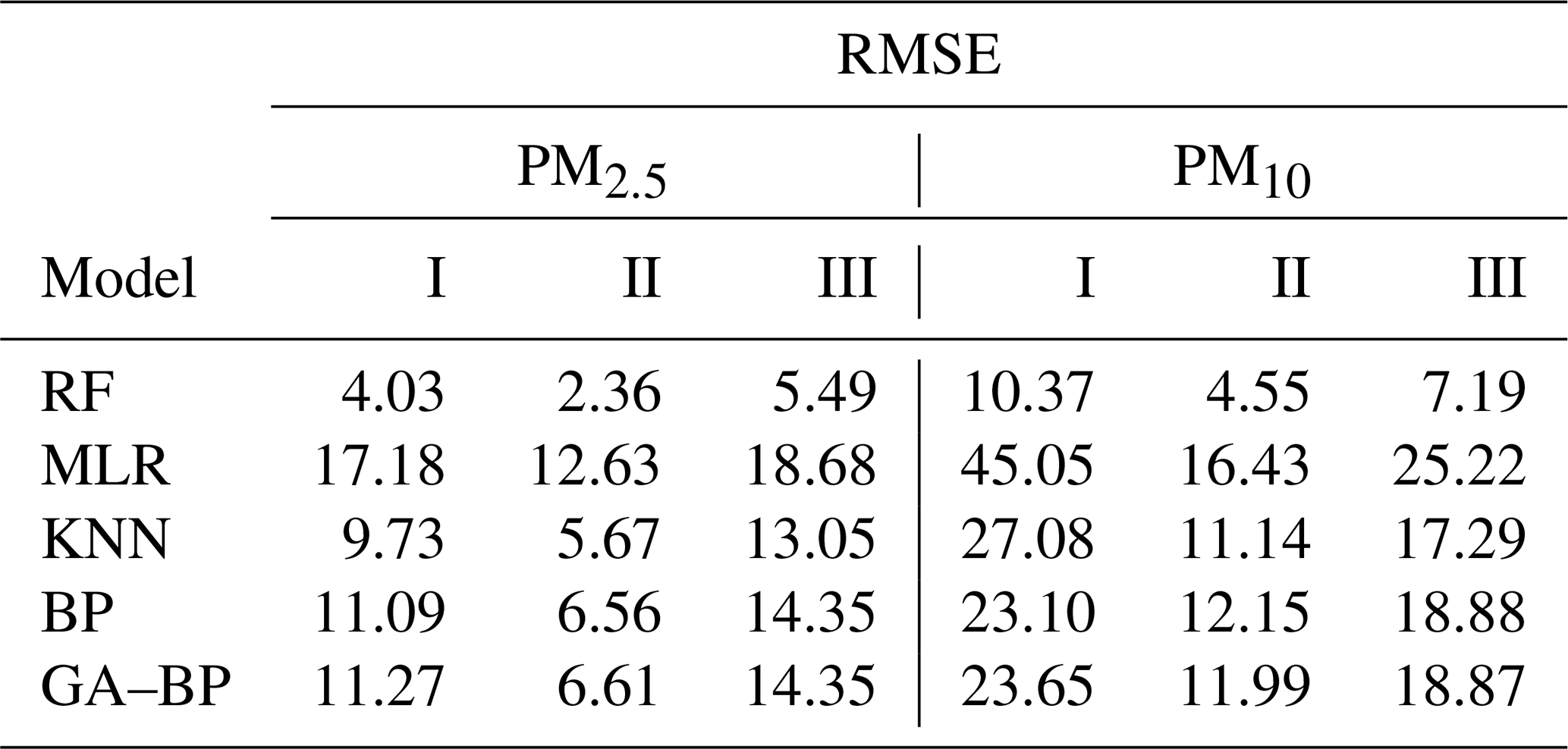
The performance of different calibration models for the PM against the reference monitor is also evaluated using RMSE, MSE, and MAE. The results are listed in Tables 3, 4, and 5, respectively. Using the data listed in Table 3, the RMSE values from the first (I) and third (III) periods are larger than the ones from the second (II) stage. The main reason may be the large fluctuation range of the PM for the climatic factors in winter and spring, resulting in the poor model fit. The RMSE values of PM2.5 between the reference data and the RF, MLR, KNN, BP, and GA–BP algorithms data are within 2.36–5.49, 12.63–18.68, 5.67–13.05, 6.56–14.35, and 6.61–14.35, respectively. The RMSE values of PM10 between the reference data and the RF, MLR, KNN, BP, and GA–BP algorithms data are calculated as 4.55–10.37, 16.43–45.05, 11.14–27.08, 12.15–23.10, and 11.99–23.65, respectively.
Table 3Performance of different calibration models for the PM2.5 and PM10 against the reference monitor. The RMSE values (lower is better) of different calibration models (RF, MLR, KNN, BP, GA–BP) versus the reference monitor.
Using the data listed in Table 4, the MAE values have the same characteristics with RMSE. The MAE values of PM2.5 between the reference data and the RF, MLR, KNN, BP, and GA–BP algorithm data are within 1.44–3.45, 8.37–12.80, 3.56–8.31, 4.46–9.55, and 4.48–9.54, respectively. The MAE values of PM10 between the reference data and the RF, MLR, KNN, BP, and GA–BP algorithm data are within 3.21–5.28, 12.21–23.20, 8.00–13.35, 8.99–15.26, and 8.89–15.43, respectively.
Table 4Performance of different calibration models for the PM2.5 and PM10 against the reference monitor. The MAE values (lower is better) of different calibration models (RF, MLR, KNN, BP, GA–BP) versus the reference monitor.
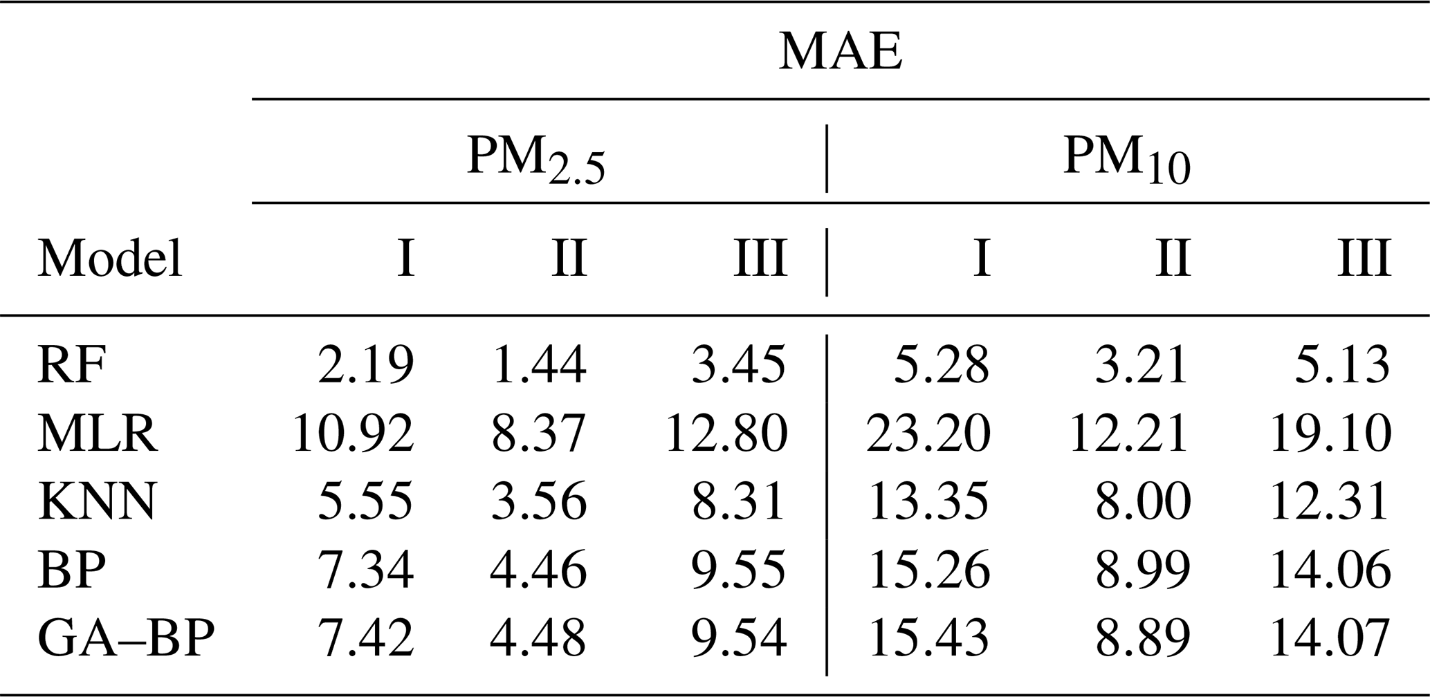
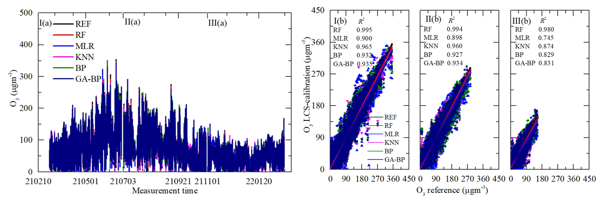
Figure 12Time series and regressions comparing the reference monitor O3 data (black) to five calibration model O3 results, where red, blue, magenta, olive, and navy represent RF, MLR, KNN, BP, and GA–BP, respectively. Panel (a) shows the whole time series data of the measurement period. Panel (b) shows the regressions of the five calibration models.
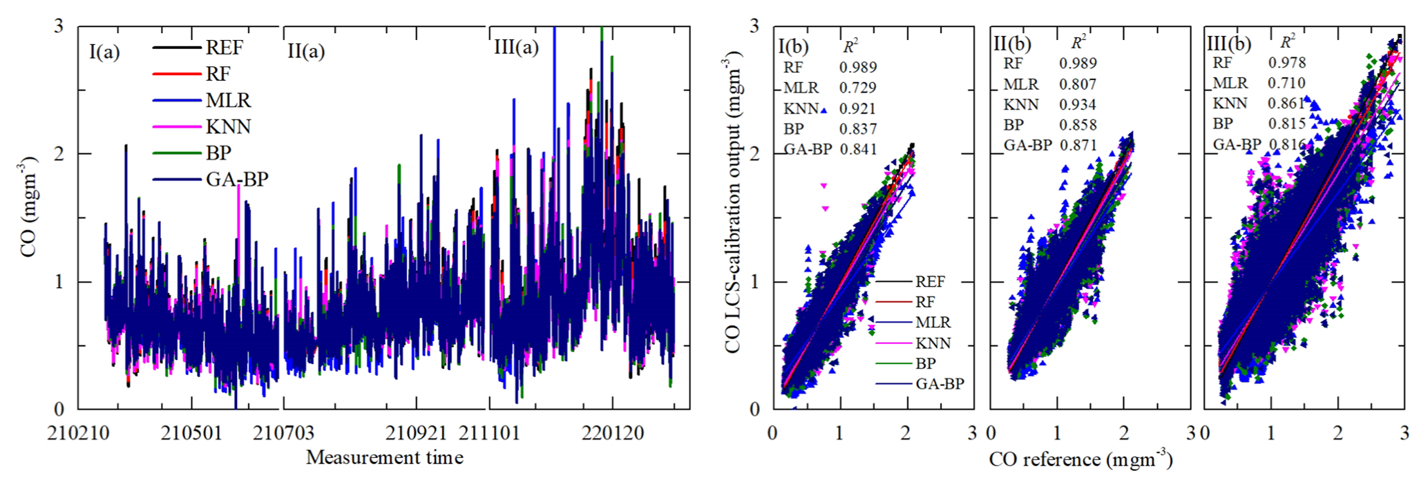
Figure 13Time series and regressions comparing the reference monitor CO data (black) to five calibration model CO results, where red, blue, magenta, olive, and navy represent RF, MLR, KNN, BP, and GA–BP, respectively. Panel (a) shows the whole time series data of the measurement period. Panel (b) shows the regressions of the five calibration models.
4.3 Measurement results of gas pollution
With the results from 1 March 2021 to 28 February 2022 and according the trend of the ambient temperature, shown in Fig. 9, the total data are also divided into three same segments as shown in Sect. 4.2. With the same purpose of avoiding over-fit in the five models and ensure the robustness of the model evaluation, the random partition parameters of train ratio and test ratio are also 80 % and 20 %, and the 5-fold cross validation is also conducted. The time series data and regressions of five modes for gas pollution from reference monitor and LCS calibration output are shown in Figs. 12–15.
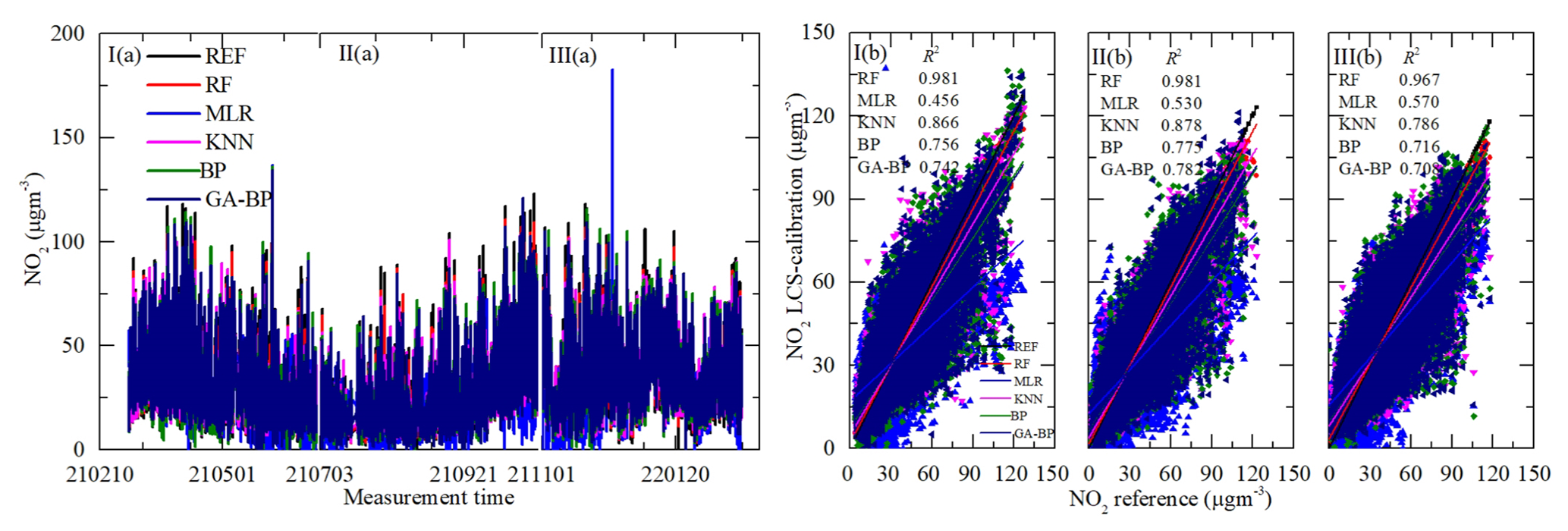
Figure 14Time series and regressions comparing the reference monitor NO2 data (black) to five calibration model NO2 results, where red, blue, magenta, olive, and navy represent RF, MLR, KNN, BP, and GA–BP, respectively. Panel (a) shows the whole time series data of the measurement period. Panel (b) shows the regressions of the five calibration models.
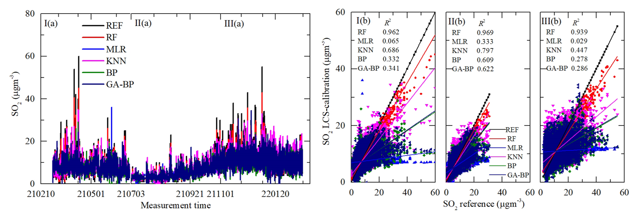
Figure 15Time series and regressions comparing the reference monitor SO2 data (black) to five calibration model SO2 results, where red, blue, magenta, olive, and navy represent RF, MLR, KNN, BP, and GA–BP, respectively. Panel (a) shows the whole time series data of the measurement period. Panel (b) shows the regressions of the five calibration models.
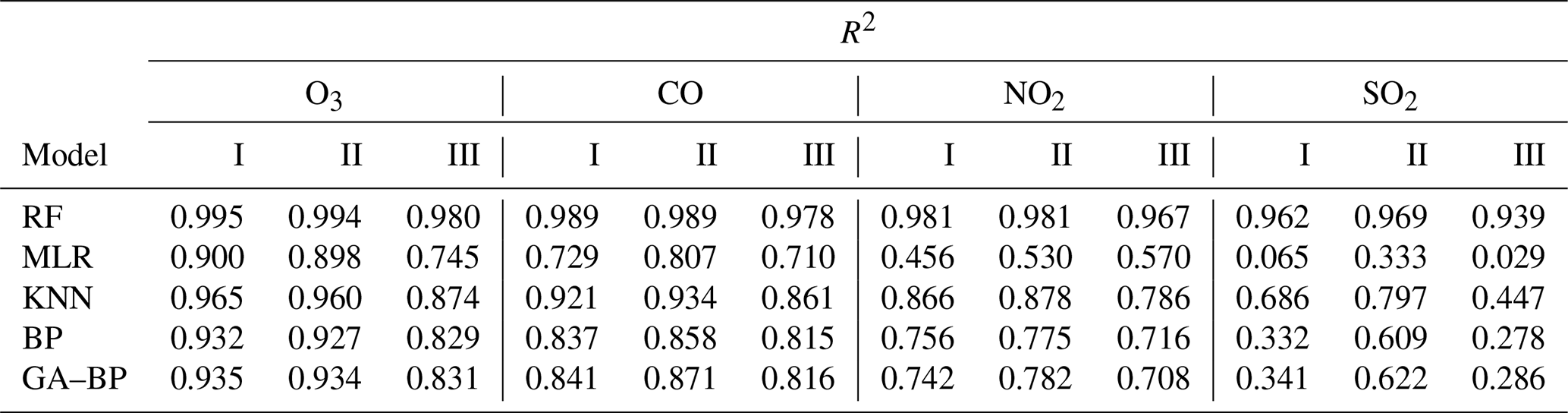
Table 5Performance of different calibration models for the gaseous pollutants (SO2, CO, NO2, and O3) against the reference monitor. The determination coefficient R2 (higher is better, maximum of 1) of different calibration models (RF, MLR, KNN, BP, GA–BP) versus the reference monitor.
As shown in Figs. 12a–15a, the general tendencies of the data fluctuation between the reference monitor and the RF, MLR, KNN, BP, and GA–BP algorithms of the LCS are consistent with each other. The RF model has the best performance, followed by KNN, BP, and GA–BP, with MLR having the worst. The R2 values between the reference data and the five model data are also shown in Figs. 12b–15b and listed in Table 5.
For the O3 model, the R2 of RF is better than 0.98. The R2 of MLR is less than 0.90 and even less than 0.8. The R2 values of the other three models are within 0.82 and 0.97. For the CO model, the R2 of RF is better than 0.97. The R2 of MLR is less than 0.81 and even less than 0.7. The R2 values of other three models are within 0.81 and 0.94. For the NO2 model, the R2 of RF is better than 0.96. The R2 of MLR is less than 0.60 and even less than 0.5. The R2 values of other three models are within 0.70 and 0.90. For the SO2 model, the R2 of RF is better than 0.93. The R2 of MLR is less than 0.40 and even less than 0.1. The R2 values of other three models are within 0.27 and 0.80.
The performances of different calibration models for the gas pollution against the reference monitor are also evaluated using RMSE and MAE. The results are listed in Tables 6 and 7, respectively.
Table 6Performance of different calibration models for the gaseous pollutants (SO2, CO, NO2, and O3) against the reference monitor. The RMSE values (lower is better) of different calibration models (RF, MLR, KNN, BP, GA–BP) versus the reference monitor.
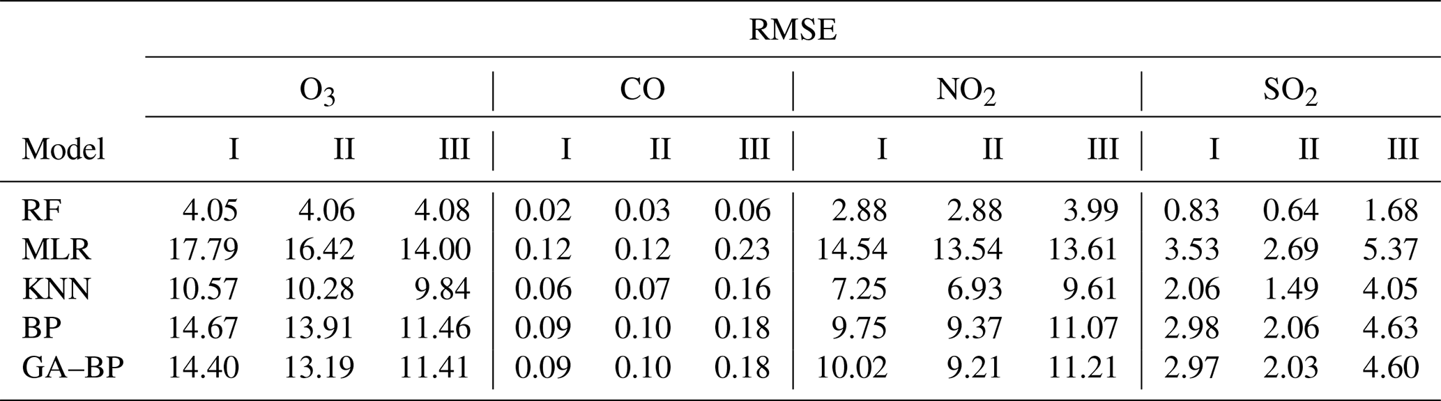
Using the data listed in Table 6, the RMSE values of O3, CO, and NO2 from the first (I) and third (III) periods have little difference with the one from the second (II) period, indicating the O3, CO, and NO2 electrochemical sensors are suitable for the ambient O3, CO, and NO2 measurements. The RMSE values of O3 between the reference data and the RF, MLR, KNN, BP, and GA–BP algorithm data are within 4.05–4.08, 14.00–17.79, 9.84–10.57, 11.46–14.67, and 11.41–14.40, respectively. The RMSE values of CO between the reference data and the RF, MLR, KNN, BP, and GA–BP algorithm data are within 0.02–0.06, 0.12–0.23, 0.06–0.16, 0.09–0.18, and 0.09–0.18, respectively. The RMSE values of NO2 between the reference data and the RF, MLR, KNN, BP, and GA–BP algorithm data are within 2.88–3.99, 13.54–14.54, 6.93–9.61, 9.37–11.07, and 9.21–11.21, respectively.
Using the RF model, the RMSE values of SO2 are better than the values of other methods but still have differences during the three periods. However, using other models, the RMSE values of SO2 from the first (I) and third (III) periods are larger than the ones from the second (II) period. The main reason may be the large ambient fluctuation for the climatic factors in winter and spring, resulting in the poor model fit. The RMSE values of SO2 between the reference data and the RF, MLR, KNN, BP, and GA–BP algorithm data are within 0.64–1.68, 2.69–5.37, 1.49–4.05, 2.06–4.63, and 2.03–4.60, respectively.
Table 7Performance of different calibration models for the gaseous pollutants (SO2, CO, NO2, and O3) against the reference monitor. The MAE values (lower is better) of different calibration models (RF, MLR, KNN, BP, GA–BP) versus the reference monitor.
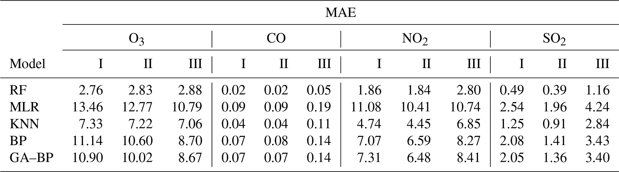
Using the data listed in Table 7, the MAE values have the same characteristics with RMSE. The MAE values of O3 between the reference data and the RF, MLR, KNN, BP, and GA–BP algorithm data are within 2.76–2.88, 10.79–13.46, 7.06–7.33, 8.70–11.14, and 8.67–10.90, respectively. The MAE values of CO between the reference data and the RF, MLR, KNN, BP, and GA–BP algorithm data are within 0.02–0.05, 0.09–0.19, 0.04–0.11, 0.07–0.14, and 0.07–0.14, respectively. The MAE values of NO2 between the reference data and the RF, MLR, KNN, BP, and GA–BP algorithm data are within 1.84–2.80, 10.41–11.08, 4.45–6.85, 6.59–8.27, and 6.48–8.41, respectively. The MAE values of SO2 between the reference data and the RF, MLR, KNN, BP, and GA–BP algorithm data are within 0.39–1.16, 1.96–4.24, 0.91–2.84, 1.41–3.43, and 1.36–3.40, respectively.
As shown in Figs. 12–15 and listed in Tables 5–7, the results of each model have little difference among the three periods for the O3, CO, and NO2 measurements, and the RF model outperforms other models.
For the data of SO2, the results of RF are better than the ones of other methods and have little difference among the three periods. However, the performances of other methods (MLR, KNN, BP, GA–BP) are poorer than the ones during the first and third periods. There may be some reasons for this phenomenon. The first one is the cross-interference effect from NO2 and O3, which have the wide range of fluctuations (from about 20 to 125 µg m−3) and increasing tendency in period I, respectively. The NO2 and SO2 can react chemically under certain conditions to produce sulfuric acid (H2SO4) and nitric acid (HNO3), which will affect the reading of SO2 sensor. The O3, highly oxidizing gas, may react with SO2 to form H2SO4 or sulfite (H2SO3), resulting in inaccurate sensor readings. The second one is the ambient temperature has a wide range of fluctuations (from about −5 to +45∘C) during the first and third periods, which will affect the stability of electrode material and the readings of the sensor. The last one is the concentration of ambient SO2 is high (more than 30 µg m−3) in period I and period III, beyond the actual measurement range of the SO2 sensor, which will be researched in future.
A low-cost air quality monitoring system (LCS) based on RF, MLR, KNN, BP, and GA–BP algorithms is proposed. The system can measure gas-phase pollutants (SO2, NO2, CO, and O3) and particle pollutants (PM2.5 and PM10), simultaneously. With the purpose of estimating the performance of the five algorithms, the LCS was mounted at the same location (Zhengzhou, China) and consistent height with the reference monitoring system. The measurement was made continuously from 1 March 2021 to 28 February 2022, with the ranges of the ambient temperature and relative humidity separately −5 to +50∘C and 10 % to 98 %, respectively. The values of the LCS and reference instruments were separately logged to the server for further comparative analysis.
With the pretreated and individual particle counters, T and RH as input, and the concentrations of PM2.5 and PM10 measured by the reference instrumentation separately as output, the multi-input single-output evaluation models based on RF, MLR, KNN, BP, and GA–BP algorithms can be obtained. With the four types of electro-chemical sensor raw data, T and RH as input, and the measurements from the reference monitors as output, the multi-input multi-output evaluation models based on the five algorithms can be obtained. The performances of the calibration models are quantitatively compared by utilizing R2, RMSE, and MAE.
The experimental results show that the R2 of RF for the PM is better than 0.98; the R2 of MLR for the PM is less than 0.91; the R2 values of the other three models are within 0.86 and 0.98. The R2 of RF for the gas pollutants (SO2, NO2, CO, and O3) is better than 0.93; the R2 of KNN, BP, and GA–BP for the gas pollutants (SO2, NO2, CO, and O3) is within 0.27 to 0.97; the R2 of MLR for the NO2, CO, and O3 is within 0.46 to 0.90, but for SO2 it is less than 0.40 and even less than 0.1.
The maximum RMSE values of PM2.5, PM10, O3, CO, NO2, and SO2 between the reference data and the RF, MLR, KNN, BP, and GA–BP algorithm data are 5.49, 18.68, 13.05, 14.35, and 14.35; 10.37, 45.05, 27.08, 23.10, and 23.65; 4.08, 17.79, 10.57, 14.67, and 14.40; 0.06, 0.23, 0.16, 0.18, and 0.18; 3.99, 14.54, 9.61, 11.07, and 11.21; and 1.68, 5.37, 4.05, 4.63, and 4.60, respectively. The maximum MAE values of PM2.5, PM10, O3, CO, NO2, and SO2 between the reference data and the RF, MLR, KNN, BP, and GA–BP algorithm data are 3.45, 12.80, 8.31, 9.55, and 9.54; 5.28, 23.20, 13.35, 15.26, and 15.43; 2.88, 13.46, 7.33, 11.14, and 10.90; 0.05, 0.19, 0.11, 0.14, and 0.14; 2.80, 11.08, 6.85, 8.27, and 8.41; and 1.16, 4.24, 2.84, 3.43, and 3.40, respectively.
It should be noted that the results of RF are better than the ones of other methods, have very good agreement with the reference monitors, and there is little difference among the three periods. However, the performances of other methods (MLR, KNN, BP, GA–BP) have poor agreement, especially during the first and third periods. There may be some reasons, such as the cross-interference effect, the wide range of fluctuation of the climatic factors, and the limitation of the actual measurement range and precision.
Overall, we conclude that, with careful data management and calibration using the machine learning algorithms, especially the RF method, these measurements are consistent with the national environmental protection standard requirement of China. The LCS may significantly improve our ability to spatial heterogeneity in air pollutant concentrations. The air pollutant maps will assist researchers, policymakers, and communities in developing new policies or mitigation strategies to enhance human health. In the next study, we will focus on improving the matching of the measurement precision and range, the generalization of the algorithms in more applications, and the performance of the SO2 sensor.
The data presented in this study are available on request by the corresponding author. The models and associated codes are not available online due to a provisional patent application.
Conceptualization: GW and CY; methodology: GW and KG; software: GW and KG; data curation: YW; Writing original draft preparation: GW; writing review and editing: KG and CY; supervision: HG. All authors have read and agreed to the published version of the manuscript.
The contact author has declared that none of the authors has any competing interests.
Publisher's note: Copernicus Publications remains neutral with regard to jurisdictional claims made in the text, published maps, institutional affiliations, or any other geographical representation in this paper. While Copernicus Publications makes every effort to include appropriate place names, the final responsibility lies with the authors.
This article is part of the special issue “In-depth study of the atmospheric chemistry over the Tibetan Plateau: measurement, processing, and the impacts on climate and air quality (ACP/AMT inter-journal SI)”. It is not associated with a conference.
The authors wish to thank Minghui Li, Hongbiao Liu, and Jinlong Wang for the helpful conversations.
This research has been supported by the National Key Research and Development Program of China (assistance agreement no. 2021YFB3200403) and Zhengzhou Education Department (grant no. 23B413006).
This paper was edited by Haichao Wang and reviewed by Alice Cavaliere and one anonymous referee.
Alexopoulos, E. C.: Inroduction to Multivariate Regression Analysis, Hippokratia, 14, 23–28, https://www.ncbi.nlm.nih.gov/pmc/articles/PMC3049417/ (last access: 12 January 2024), 2010.
Ali, S., Glass, T., Parr, B., Potgieter, J., and Alam, F.: Low Cost Sensor With IoT LoRaWAN Connectivity and Machine Learning-Based Calibration for Air Pollution Monitoring, IEEE T. Instrum. Meas., 70, 5500511, https://doi.org/10.1109/TIM.2020.3034109, 2021.
Amuthadevi, C., Vijayan, D. S., and Ramachandran, V.: Development of air quality monitoring (AQM) models using different machine learning approaches, J. Amb. Intel. Hum. Comp., 13, 33, https://doi.org/10.1007/s12652-020-02724-2, 2021.
Ari, D. and Alagoz, B. B.: An effective integrated genetic programming and neural network model for electronic nose calibration of air pollution monitoring application, Neural Comput. Appl., 34, 12633–12652, https://doi.org/10.1007/s00521-022-07129-0, 2022.
Bakiler, H. and Guney, S.: Estimation of Concentration Values of Different Gases Based on Long Short-Term Memory by Using Electronic Nose, Biomed. Signal Proces., 69, 102908, https://doi.org/10.1016/j.bspc.2021.102908, 2021.
Breiman, L.: Random Forests, Mach. Learn., 45, 5–32, https://doi.org/10.1023/A:1010933404324, 2001.
Chai, T. and Draxler, R. R.: Root mean square error (RMSE) or mean absolute error (MAE)? – Arguments against avoiding RMSE in the literature, Geosci. Model Dev., 7, 1247–1250, https://doi.org/10.5194/gmd-7-1247-2014, 2014.
Cross, E. S., Williams, L. R., Lewis, D. K., Magoon, G. R., Onasch, T. B., Kaminsky, M. L., Worsnop, D. R., and Jayne, J. T.: Use of electrochemical sensors for measurement of air pollution: correcting interference response and validating measurements, Atmos. Meas. Tech., 10, 3575–3588, https://doi.org/10.5194/amt-10-3575-2017, 2017.
Cui, H., Zhang, L., Li, W., Yuan, Z., Wu, M., Wang, C., and Ma, J.: A new calibration system for low-cost Sensor Network in air pollution monitoring, Atmos. Pollut. Res., 12, 101049, https://doi.org/10.1016/j.apr.2021.03.012, 2021.
Esposito, E., De, V. S., Salvato, M., Bright, V., Jones, R. L., and Popoola, O.: Dynamic neural network architectures for on field stochastic calibration of indicative low cost air quality sensing systems, Sensor. Actuat. B-Chem., 231, 701–713, https://doi.org/10.1016/j.snb.2016.03.038, 2016.
Goh, C. C., Kamarudin, L. M., Zakaria, A., Nishizaki, H., Ramli, N., Mao, X., Syed Zakaria, S. M. M., Kanagaraj, E., Abdull Sukor, A. S., and Elham, M. F.: Real-Time In-Vehicle Air Quality Monitoring System Using Machine Learning Prediction Algorithm, Sensors, 21, 4956, https://doi.org/10.3390/s21154956, 2021.
Hitchman, M. L., Cade, N. J., Gibbs, T. K., and Hedley, N. J. M.: Study of the factors affecting Mass Transport in Electrochemical Gas Sensors, Analyst, 122, 1411–1417, https://doi.org/10.1039/a703644b, 1997.
Ionascu, M. E., Castell, N., Boncalo, O., Schneider, P., Darie, M., and Marcu, M.: Calibration of CO, NO2, and O3 Using Airify: A Low-Cost Sensor Cluster for Air Quality Monitoring, Sensors, 21, 7997, https://doi.org/10.3390/s21237977, 2021.
Janabi, S. A., Alkaim, A., Al-Janabi, E., Aljeboree, A., and Mustafa, M.: Intelligent forecaster of concentrations (PM2.5, PM10, NO2, CO, O3, SO2)3 caused air pollution (IFCsAP), Neural Comput. Appl., 33, 14199–14229, https://doi.org/10.1007/s00521-021-06067-7, 2021.
Jiao, W., Hagler, G., Williams, R., Sharpe, R., Brown, R., Garver, D., Judge, R., Caudill, M., Rickard, J., Davis, M., Weinstock, L., Zimmer-Dauphinee, S., and Buckley, K.: Community Air Sensor Network (CAIRSENSE) project: evaluation of low-cost sensor performance in a suburban environment in the southeastern United States, Atmos. Meas. Tech., 9, 5281–5292, https://doi.org/10.5194/amt-9-5281-2016, 2016.
Khreis, H., Johnson, J., Jack, K., Dadashova, B., and Park, E. S.: Evaluating the Performance of Low-Cost Air Quality Monitors in Dallas, Texas, Int. J. Env. Res. Pub. He., 19, 1647, https://doi.org/10.3390/ijerph19031647, 2022.
Kumar, T.: Solution of Linear and Non Linear Regression Problem by K Nearest Neighbour Approach: By Using Three Sigma Rule, 2015 IEEE International Conference on Computational Intelligence & Communication Technology, 13–14 February 2015, Ghaziabad, India, IEEE, 197–201, https://doi.org/10.1109/CICT.2015.110, 2015.
Liang, Y., Ren, C., Wang, H., Huang, Y., and Zheng, Z.: Research on soil moisture inversion method based on GA-BP neural network model, Int. J. Remote Sens., 40, 2087–2103, https://doi.org/10.1080/01431161.2018.1484961, 2018.
Liu, Y., Wang, Y., and Zhang, J.: New machine learning algorithm: Random forest. Information Computing and Applications, ICICA 2012, Springer, Berlin, Heidelberg, 7473, 246–252, https://doi.org/10.1007/978-3-642-34062-8_32, 2012.
Mahesh, T. R., Vinoth, K. V., Dhilip, K. V., Oana, G., Martin, M., and Manisha, G.: The stratified K-folds cross-validation and class-balancing mehtods with high-performance ensemble classifiers for breast cancer classification, Healthcare Analytics, 2023, 100247, https://doi.org/10.1016/j.health.2023.100247, 2023.
Manisalidis, I., Stavropoulou, E., Stavropoulos, A., and Bezirtzoglou, E.: Environmental and Health Impacts of Air Pollution: A Review, Frontiers in Public Health, 8, 1–13, https://doi.org/10.3389/fpubh.2020.00014, 2020.
Masson, N., Piedrahita, R., and Hannigan, M.: Quantification method for electrolytic sensors in long-term monitoring of ambient air quality, Sensors, 15, 27283–27302, https://doi.org/10.3390/s151027283, 2015.
Mead, M. I., Popoola, O. A. M., Stewart, G. B., and Landshoff, P.: The use of electro-chemical sensors for monitoring urban air quality in Low-cost, high-density networks, Atmos. Environ., 70, 186–203, https://doi.org/10.1016/J.ATMOSENV.2012.11.060, 2013.
Ministry of Ecology and Environment of the People's Republic of China: Technical specifications for operation and quality control of ambient air quality continuous automated monitoring system for SO2, NO2, O3 and CO, China Environment Publishing Group, HJ 818 2018, https://www.mee.gov.cn/ywgz/fgbz/bz/bzwb/jcffbz/201808/W020180815358674459089.pdf (last access: 13 January 2024), 2018.
Ministry of Ecology and Environment of the People's Republic of China: Technical guide for automatic monitoring by beta ray method for particulate matter in ambient air (PM10 and PM2.5), China Environment Publishing Group, HJ 1100 2020, https://www.mee.gov.cn/ywgz/fgbz/bz/bzwb/other/qt/202002/W020200218580781246278.pdf (last access: 13 January 2024), 2020.
Ning, M., Guan, J., Liu, P., Zhang, Z., and O'Hare, G. M. P.: GA-BP Air Quality Evaluation Method Based on Fuzzy Theory, CMC-Comp. Mater. Con., 58, 215–227, https://doi.org/10.32604/cmc.2019.03763, 2019.
Rezaei, R., Naderalvojoud, B., and Güllü, G.: A Comparative study of Deep Learning Models on Tropospheric Ozone Forecasting Using Feature Engineering Approach, Atmosphere, 14, 239, https://doi.org/10.3390/atmos14020239, 2023.
Singh, A., Ng'ang'a, D., Gatari, M. J., Kidane, A. W., Alemu, Z. A., Derrick, N., and Webster, M. J.: Air quality assessment in three East African cities using calibrated low-cost sensors with a focus on road-based hotspots, Environmental Research Communications, 3, 075007, https://doi.org/10.1088/2515-7620/ac0e0a, 2021.
Spinelle, L., Gerboles, M., Villani, M. G., Aleixandre, M., and Bonavitacola, F.: Field calibration of a cluster of low-cost available sensors for air quality monitoring. Part A: Ozone and nitrogen dioxide, Sensor. Actuat. B-Chem., 215, 249–257, https://doi.org/10.1016/j.snb.2015.03.031, 2015.
Spinelle, L., Gerboles, M., Villani, M. G., Aleixandre, M., and Bonavitacola, F.: Field calibration of a cluster of low-cost commercially available sensors for air quality monitoring. Part B: NO, CO and CO2, Sensor. Actuat. B-Chem., 238, 706–715, https://doi.org/10.1016/j.snb.2016.07.036, 2017.
Wang, C., Pan, B., Wu, X., Song, Y., Zhang, L., Ma, J., and Sun, K.: Research on Quality Control of Atmospheric Grid Monitoring Based on Large Data Analysis, Environmental Monitoring in China, 32, 1–6, https://doi.org/10.19316/j.issn.1002-6002.2016.06.01, 2016.
Wang, S., Li, L., Ma, W., and Chen, X.: Trajectory analysis for on-demand services: A survey focusing on spatial-temporal demand and supply patterns, Transport. Res. C-Emer., 108, 74–99, https://doi.org/10.1016/j.trc.2019.09.007, 2019.
Wei, P., Ning, Z., Ye, S., Sun, L., and Yang, F.: Impact Analysis of Temperature and Humidity Conditions on Electrochemical Sensor Response in Ambient Air Quality Monitoring, Sensors, 18, 59, https://doi.org/10.3390/s18020059, 2018.
Xu, X., Guo, H., and Fan, J.: Water quality evaluation of Xiaoshan water quality station in eastern Zhejiang Water Diversion Project Based on BP network, J. Phys. Conf. Ser., 1732, 012035, https://doi.org/10.1088/1742-6596/1732/1/012035, 2021.
Zhao, C., Wang, Y., Shi, X., Zhang, D., Wang, C., Jiang, J., and Zhang, Q.: Estimating the Contribution of Local Primary Emissionsto Particulate Pollution Using High-Density Station Observations, J. Geophys. Res.-Atmos., 124, 1648–1661, https://doi.org/10.1029/2018JD028888, 2019.
Zhao, P. and Lai, L.: Minimax Rate Optimal Adaptive Nearest Neighbor Classification and Regression, IEEE T. Inform. Theory, 67, 3155–3182, https://doi.org/10.1109/TIT.2021.3062078, 2021.
Zhu, N., Zhu, C., Zhou, L., Zhu, Y., and Zhang, X.: Optiminzation of the Random Forest Hyperparameters for Power Industrial Control Systems Intrusion Detection Using an Improved Grid Search Algorithm, Appl. Sci., 12, 10456, https://doi.org/10.3390/app122010456, 2022.
Zimmerman, N., Presto, A. A., Kumar, S. P. N., Gu, J., Hauryliuk, A., Robinson, E. S., Robinson, A. L., and R. Subramanian: A machine learning calibration model using random forests to improve sensor performance for lower-cost air quality monitoring, Atmos. Meas. Tech., 11, 291–313, https://doi.org/10.5194/amt-11-291-2018, 2018.
Zoest, V. V., Osei, F. B., Stein, A., and Hoek, G.: Calibration of low-cost NO2 sensors in an urban air quality network, Atmos. Environ., 210, 66–75, https://doi.org/10.1016/j.atmosenv.2019.04.048, 2019.