Design and evaluation of a low-cost sensor node for near-background methane measurement

We developed a low-cost methane sensing node incorporating two metal oxide (MOx) sensors (Figaro Engineering TGS2611-E00 and TGS2600), humidity and temperature sensing, data storage, and telemetry. We deployed the prototype sensor alongside a reference methane analyzer at two sites: one outdoors and one indoors. We collected data at each site for several months across a range of environmental conditions (particularly temperature and humidity) and methane levels. We explored calibration models to investigate the performance of our system and its suitability for methane background monitoring and enhancement detection, first selecting a linear regression to fit a sensor baseline response and then fitting methane response by the sensor deviation from baseline. We achieved moderate accuracy in a 2 to 10 ppm methane range compared to data from the reference analyzer (RMSE < 0.6 ppm), but we found that the sensor response varied over time, possibly as a result of changes in non-targeted gas concentrations. We suggest that this cross sensitivity may be responsible for mixed results in previous studies. We discuss the implications of our results for the use of these and similar inexpensive MOx sensors for methane monitoring in the 2 to 10 ppm range.

1 Introduction

With the well-known importance of methane emissions to climate change, scientists and engineers are working to develop low-cost sensor networks and monitoring methods, with motivations and applications summarized by Aldhafeeri et al. (2020). Researchers and commercial entities have explored a variety of sensor mechanisms for methane, including optical, pyroelectric, and chemiresistive devices, among others (Aldhafeeri et al., 2020). Due to their low cost, metal oxide (MOx) semiconductor sensor elements are appealing candidates for inexpensive sensor network development (Cho et al., 2022).

MOx sensor implementation poses a variety of technical challenges, and laboratory calibrations may not translate to real-world applications (Barsan et al., 2007). In particular, environmental factors such as humidity and interfering gasses are difficult to incorporate in a lab setting (Wang et al., 2010). Poor selectivity for target gasses is a challenge of particular relevance to our current study; this is a well-known problem with a variety of possible solutions, including sensor array or “e-nose” configurations in which a set of sensors with different target gasses are used as an ensemble to identify the species in gas compositions (Ponzoni et al., 2017; Cheng et al., 2021).

A variety of previous studies have explored the TGS MOx sensor product line from Figaro Engineering for methane detection. In particular, the TGS2600 and TGS2611-E00 sensors have promising reports in the literature (Collier-Oxandale et al., 2018; van den Bossche et al., 2017). The TGS2611-E00 is marketed for methane detection in alarms, leak monitoring, and similar applications (Figaro USA, Inc., 2013); the TGS2600 is marketed as a general-purpose air contaminant sensor for use in air quality monitors and similar devices (Figaro USA, Inc., 2022b). Both are low-cost sensing elements available for around USD 20 each from electronic component distributors (Maritex Co., September 2023 prices).

Previous work has found TGS2611-E00 to perform reasonably well when calibrated and tested in a laboratory setting, with error within ±1.7 ppm across a 2 to 9 ppm methane concentration (van den Bossche et al., 2017). Several field experiments have found useful performance for detecting methane concentrations in a higher range; among them, Cho et al. (2022) found TGS2611-E00 effective above 100 ppm concentrations in a laboratory calibration and field experiment, and Jørgensen et al. (2020) reported success in the 2 to 100 ppm range in the field. Riddick et al. (2022) successfully detected large changes in methane concentrations, corresponding to natural gas leaks. Shah et al. (2023) provided an in-depth examination of TGS2611-E00 calibration, including the important observation that laboratory calibrations may not generalize to different ambient conditions in the field. All of the previous studies note that environmental conditions, particularly humidity levels, affect sensor response; Shah et al. (2023) also provided some evidence that ambient gas makeup plays a significant role in sensor behavior.

TGS2600 has also found positive results for methane detection in some studies. Eugster and Kling (2012) reported a general sensor correspondence with methane trends in a field study, although with a low R² of 0.19. Other papers found better performance (Collier-Oxandale et al., 2018; Riddick et al., 2020; Eugster et al., 2020; Casey et al., 2019) but generally with complicated algorithms required and in some cases with notable differences in performance between laboratory and field settings (Riddick et al., 2020) or from site to site (Collier-Oxandale et al., 2018).

The previously mentioned studies explore a range of methane concentrations. We focus in this paper on a low concentration range, which we define as ranging from the atmospheric background of approximately 2 to 10 ppm. Our previous laboratory work suggests that TGS2611-E00 has some methane response in this range and that TGS2600 does not (Furuta et al., 2022). It is unclear from previously published work whether these sensors are viable for monitoring the 2 to 10 ppm range in real-world settings and whether these sensors are therefore usable in low-cost sensing networks for monitoring small fugitive emissions and similar low-concentration applications.

To better understand the viability of low-cost MOx sensors for monitoring methane in this low concentration range, we designed an inexpensive sensor node complete with telemetry and data logging, deployed the node in an outdoor setting and an indoor setting with a range of methane concentrations for several months each, and then characterized the sensor response to both environmental conditions and methane levels. We present the full design for our sensor node and mention its strengths and shortcomings. We highlight several difficulties in monitoring this low methane concentration range with MOx sensors, and we discuss the suitability of the sensing approach for the concentration range of interest.

2 Methods

2.1 Sensing system design

We designed and built a system consisting of two MOx sensors, a relative humidity and temperature sensor, data storage and telemetry, and power supplies and interfacing circuitry. We implemented the system on two printed circuit boards (PCBs), with one PCB holding the sensors and associated circuitry and the other PCB holding the data storage and telemetry components, as described in full in Appendix A. The total parts cost of our system was under USD 200.

We chose TGS2611-E00 (Figaro USA, Inc., 2013) and TGS2600 (Figaro USA, Inc., 2022b) MOx sensors from Figaro Engineering Inc. as our primary sensing elements. Based on our previous work, we expected TGS2611-E00 to respond reasonably well to methane and TGS2600 to show a weak or no response to methane in the concentration range of interest (Furuta et al., 2022). By including both sensors, we hoped to allow our calibration algorithm to compensate for non-methane interfering gasses that might be detected by both TGS2600 and TGS2611-E00.

TGS2611-E00 is designed with an integrated filter, which is intended to remove interfering gasses such as alcohol (Figaro USA, Inc., 2013). TGS2600 has no such filter. According to the manufacturer, TGS2611-E00 is sensitive to methane, hydrogen, and ethanol, in order of magnitude of response (Figaro USA Inc., 2023); TGS2600 is sensitive to hydrogen, ethanol, iso-butane, carbon monoxide, and methane, again in order of sensitivity (Figaro USA Inc., 2022a). Accordingly, including both sensors may help to reduce the effect of hydrogen, ethanol, or other interfering gasses not characterized by the manufacturer, although iso-butane, carbon monoxide, or other unknown gasses might cause a response in TGS2600 that is not present in TGS2611-E00.

MOx sensors require stable power supplies for accurate readings, with previous studies noting that power supply fluctuations compromise performance (van den Bossche et al., 2017; Shah et al., 2023). Our overall system ran from a 5 V DC power supply; to ensure high stability for the sensing elements, we operated them at 4.8 V derived from an onboard precision voltage regulator. We burned in the sensors and regulator for a week prior to data collection to allow any initial reactions in the sensing elements or the sensors' internal heaters to stabilize, as well as to ensure the system was stable and functioning properly before deployment.

MOx sensors vary in resistance in response to target gasses, as well as in response to interfering gasses, water vapor, and other factors. To convert this variation to a voltage signal that could be easily digitized, we placed the sensors in voltage divider configurations against selected reference resistors. For maximum sensitivity, the reference resistance value should be close to the expected sensor resistance; we used results from our previous work to choose reference resistor values of 15 kΩ for TGS2600 and 75 kΩ for TGS2611-E00 (Furuta et al., 2022). We digitized the voltage output for each divider using an ADS1115 16-bit analog-to-digital converter (Texas Instruments, Inc.).

To confirm power supply stability, we also digitized the sensor power supply voltage. Our system performed well in both sections of the experiment, with 95 % of all data showing a sensor supply voltage within ±0.25 mV of the mean and 99.99 % of all data showing a supply voltage within ±0.80 mV of the mean across the full dataset.

We recorded relative humidity and temperature using an SHT31-DIS sensor (Sensirion AG), which produced digitized readings with 2 % relative humidity accuracy and 0.2 °C temperature accuracy.

An M0 Adalogger microcontroller module (Adafruit Industries) controlled the overall system and recorded readings every 5 to 6 s to an SD card. We used a Boron microcontroller module (Particle Industries, Inc.) as a cellular modem for telemetry; the Boron module also provided accurate timestamps for the data logger. The microcontroller module included a cellular data service sufficient for our needs without recurring cost. We found one brief period of corrupted readings, likely due to SD card malfunctioning, which we removed from the dataset. We did not note any other obvious problems with the system functioning.

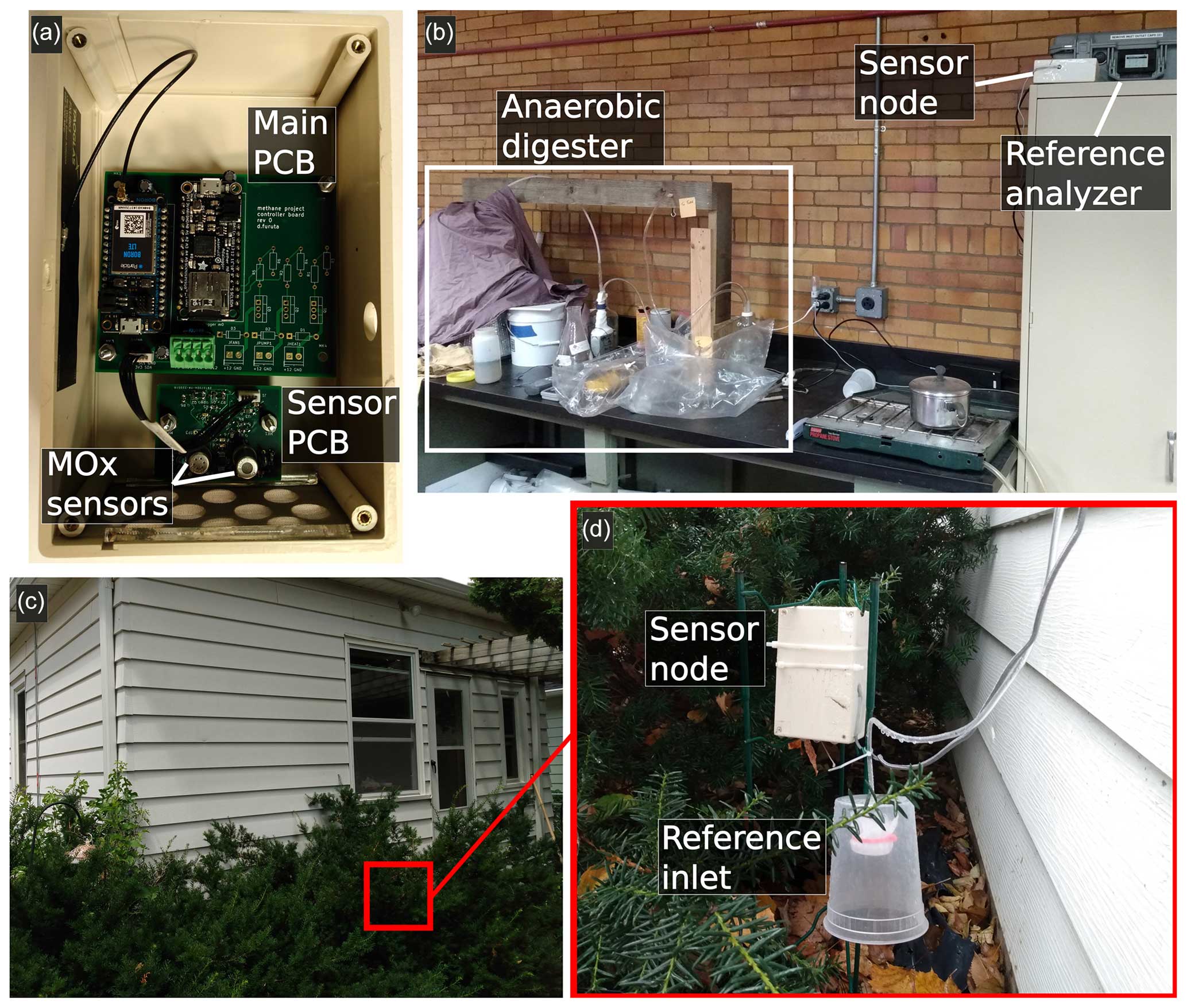
Figure 1 Panel (a) shows the sensor node construction, which is described fully in Appendix A. Panel (b) is the indoor study site with the sensor node and reference analyzer placed close to a demonstration anaerobic digester. Panel (c) is the outdoor study site, with panel (d) showing the positioning of the sensor node and reference analyzer intake.

We mounted the electronics inside a small enclosure with holes cut to allow air entry, as seen in Fig. 1a. We screened the opening to prevent debris, insects, or other objects from entering the case. Our system operated passively, without an air pump. The passive operation caused some lag in the sensor response, as described further in Appendix A; the system responded within minutes to a large methane enhancement but took considerably longer to return to baseline afterwards.

We provide full schematics and a detailed electronic description of the sensing system in Appendix A.

2.2 Experimental design

We characterized the sensing system at two different sites, with a co-located LI-7810 methane analyzer (LI-COR, Inc.) as a reference device. The LI-7810 monitors methane, water vapor, and CO₂ using optical spectroscopy with precision better than 1 ppb for methane and 50 ppm for water vapor, with a frequency of one reading per second (LI-COR Inc., 2023). We did not use the CO₂ measurements for this paper. Figure 1 depicts the experimental sites and setup.

2.2.1 Outdoor site: ambient levels with short controlled releases

Our first site was an urban yard in the Cooper neighborhood of Minneapolis without any notable known sources of methane or interfering gasses nearby; our intention for this site was to characterize our sensor's performance close to background methane levels. We located our sensing system and the reference analyzer's sample intake near the house exterior, as seen in Fig. 1c and d. The reference analyzer drew samples through approximately 3 m of tubing: as we later averaged the data to a 10 min timescale, we considered the resulting sampling lag of less than 30 s to be negligible for the purpose of our analysis.

The background methane concentration at our research site as measured by the LI-7810 was approximately 2 ppm, with a minimum observation of 1.98 ppm. We had no expectation of elevated levels. To provide some range of methane concentrations, we performed a small number of controlled releases in the vicinity of our sensor setup from a 2.5 % methane gas cylinder balanced with air. In August 2022 we released methane eight times through a 2 L min⁻¹ regulator for 30 s each and once for 15 s. In October and November 2022 we released methane 40 times through a 0.1 L min⁻¹ regulator for 10 min each. These releases produced a maximum 10 min averaged methane value of 5.8 ppm, with most of the releases producing methane concentrations between 3 and 4.5 ppm as measured by the reference analyzer.

2.2.2 Indoor site: methane leaks and elevated levels

Our second site was indoors in the Biosystems Engineering building at the University of Minnesota, Twin Cities campus, approximately 5 km from our outdoor site. We placed our sensing system and reference analyzer close to a benchtop classroom-scale demonstration anaerobic digester, as shown in Fig. 1b, with the reference analyzer drawing air from directly next to the sensor node. The digester was located in a large workshop area, and we expected a variety of methane levels resulting from small leaks or larger pulses when biomass was added to the digester or when methane was removed. We also expected possible emissions of methane, VOCs, hydrogen sulfide, and nitrous oxide along with other unknown gasses from surrounding labs, some of which were working on fermentation, manure processing, and other bioprocessing projects. Since this site was indoors, we expected a narrower range of temperatures and humidities than at our outdoor site.

We collected data from the outside site from July to November 2022 and from the indoors site from January to May 2023.

2.3 Data processing

The reference analyzer showed clock drift over the sampling periods, which we noted and corrected. We converted the raw MOx sensor readings to resistance values using the recorded supply voltages and known voltage divider resistor values. We associated the reference and sensor data by their timestamps.

The indoor portion of data collection saw several large, short methane spikes which exceeded the specified range of the reference analyzer; as we were unable to guarantee data quality in these periods, we dropped all data within a 1 h window of a methane value exceeding the reference analyzer upper limit of 100 ppm. We chose the relatively long window to ensure that both the reference analyzer and sensor node had returned to baseline conditions after each spike. The outside experiment lost records from the reference analyzer for 2 weeks, leading to a gap in the data. Our sensor experienced power failures on several occasions through the experiment, as well as sporadic downtime to allow for data retrieval. As the MOx sensors have internal heaters which require some time to stabilize, we removed 2 h of data after each reboot; we illustrate the full warm-up behavior in Appendix A.

To reduce the effect of any lag between our passive sensor node and the active-sampling reference analyzer and to smooth any extremely short-duration spikes that our diffusion-based sensor node might fail to capture, we chose to perform our analysis on the dataset averaged in consecutive 10 min values.

Our research interest is the low methane concentration range, which we define as background to 10 ppm, with a background concentration of approximately 2 ppm in our location. We removed averaged data with concentrations above 10 ppm as well as the data immediately following; this resulted in removing 31 of 15 688 records for the inside set and 3 of 14 333 records for the outside set.

2.4 Sensor calibration

MOx sensors have well-known sensitivities to water vapor and other environmental conditions. Previous studies, as well as manufacturer data sheets, have often related methane to the sensor response using a baseline value, which represents the expected sensor response to environmental conditions other than methane (Figaro USA, Inc., 2013; Eugster and Kling, 2012; Riddick et al., 2022; Shah et al., 2023). Methane is then fit by an equation using the sensor deviation from the expected baseline value. We proceeded with this two-step approach as follows.

First, we estimated the baseline TGS2611-E00 sensor response without methane enhancements by fitting the response as a function of environmental conditions for time periods where the measured methane concentration was below 2.3 ppm. We chose 2.3 ppm a priori as a threshold below which the sensors should be unable to detect methane changes based on our prior work (Furuta et al., 2022). We examined the effect of several environmental parameters: temperature, water vapor concentration, and elapsed sensor running time. We chose to include sensor run time to incorporate any effects of sensor aging, defining run time as the total time the sensor was switched on since the beginning of the experiment; this time parameter also potentially included any effects from other environmental parameters we were not equipped to measure, such as interfering, non-target gasses.

Our experiment collected both water vapor concentrations and relative humidity data from the reference analyzer and a PCB-mounted sensor, respectively. Relative humidity is dependent on water vapor concentrations and temperature, as well as atmospheric pressure, and our previous work found water vapor concentrations to predict sensor response better than relative humidity (Furuta et al., 2022); accordingly, we decided a priori to include water vapor concentrations, as measured by the LI-7810, and not relative humidity as a possible term in our analysis. This decision is further supported by previous work, as described in Shah et al. (2023).

After evaluating the possible regressions, we selected Eq. (1) as the best-performing fit for the TGS2611-E00 baseline across the inside, outside, and combined datasets, again fitting only data with methane concentrations below 2.3 ppm. We provide a detailed description of the equation selection process in Appendix B.

$$\begin{array}{}\text{(1)}& \log \left(\mathrm{baseline}\right)={\mathit{\beta }}_{\mathrm{0}}+{\mathit{\beta }}_{\mathrm{1}}\log \left({\mathrm{H}}_{\mathrm{2}}\mathrm{O}\right)+{\mathit{\beta }}_{\mathrm{2}}T+{\mathit{\beta }}_{\mathrm{3}}\log \left(\mathrm{time}\right)\end{array}$$

Our sensing system included a secondary sensor, the TGS2600, which we previously found to not respond to methane in the concentration range of interest (Furuta et al., 2022). We examined whether including this sensor in the baseline prediction could improve accuracy, most likely by accounting for non-target interfering gasses. Adding this sensor to Eq. (1) produced Eq. (2) as a possibly improved candidate for the baseline regression.

$$\begin{array}{}\text{(2)}& \begin{array}{rl}\log \left(\mathrm{baseline}\right)& ={\mathit{\beta }}_{\mathrm{0}}+{\mathit{\beta }}_{\mathrm{1}}\log \left({\mathrm{H}}_{\mathrm{2}}\mathrm{O}\right)+{\mathit{\beta }}_{\mathrm{2}}T\\ & +{\mathit{\beta }}_{\mathrm{3}}\log \left(\mathrm{time}\right)+{\mathit{\beta }}_{\mathrm{4}}\log \left(\mathrm{TGS}\mathrm{2600}\right)\end{array}\end{array}$$

The TGS2611-E00 sensor response is expected to deviate from the predicted baseline response as a result of methane levels. Over a large range, this deviation will likely take the form of a power function (Shah et al., 2023); however, in the limited range we examined we chose a linear fit for simplicity as shown in Eq. (3a). We rearrange this equation to predict methane levels in Eq. (3b).

$$\begin{array}{}\text{(3a)}& {\displaystyle \frac{\mathrm{TGS}\mathrm{2611}}{\mathrm{baseline}}}=\mathit{\alpha }+\mathit{\beta }{\mathrm{CH}}_{\mathrm{4}},\text{(3b)}& {\displaystyle }{\mathrm{CH}}_{\mathrm{4}}={\displaystyle \frac{\mathrm{1}}{\mathit{\beta }}}{\displaystyle \frac{\mathrm{TGS}\mathrm{2611}}{\mathrm{baseline}}}-{\displaystyle \frac{\mathit{\alpha }}{\mathit{\beta }}}.\end{array}$$

We used the combination of Eq. (3) with either Eq. (1) or Eq. (2) to calibrate the TGS2611-E00 response to methane. We evaluated the performance of each component as well as examined challenges for the calibration method.

3 Results

3.1 Collected data

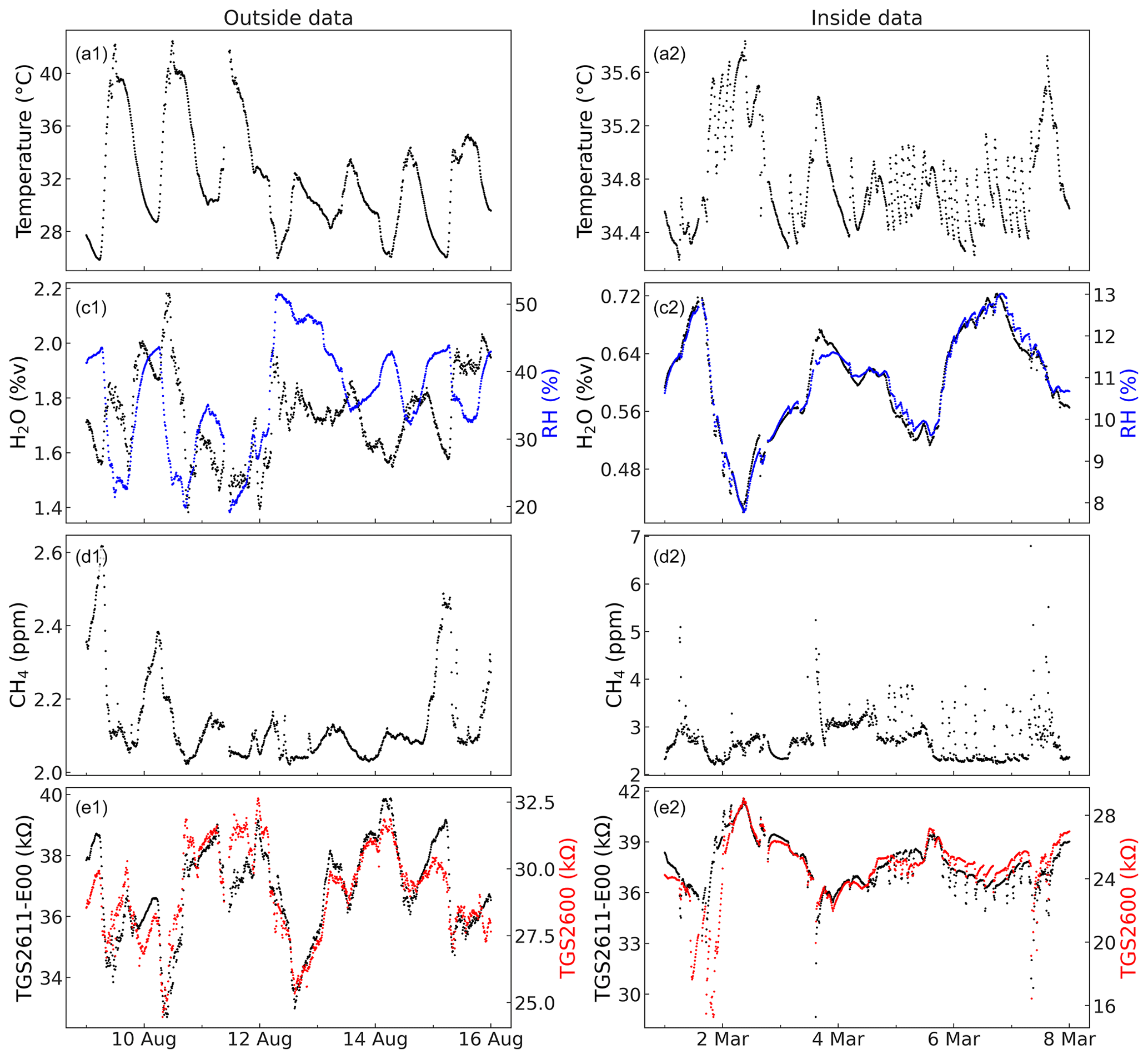
Figure 2 plots the time series of cleaned, 10 min averaged data for the two experiments. As mentioned previously, data loss from the reference analyzer led to a 2-week gap in late August and early September. Both experiments had occasional smaller gaps not visible on the plots due to power failures, system downtime for data collection, methane spikes exceeding the reference analyzer specifications, and similar causes.

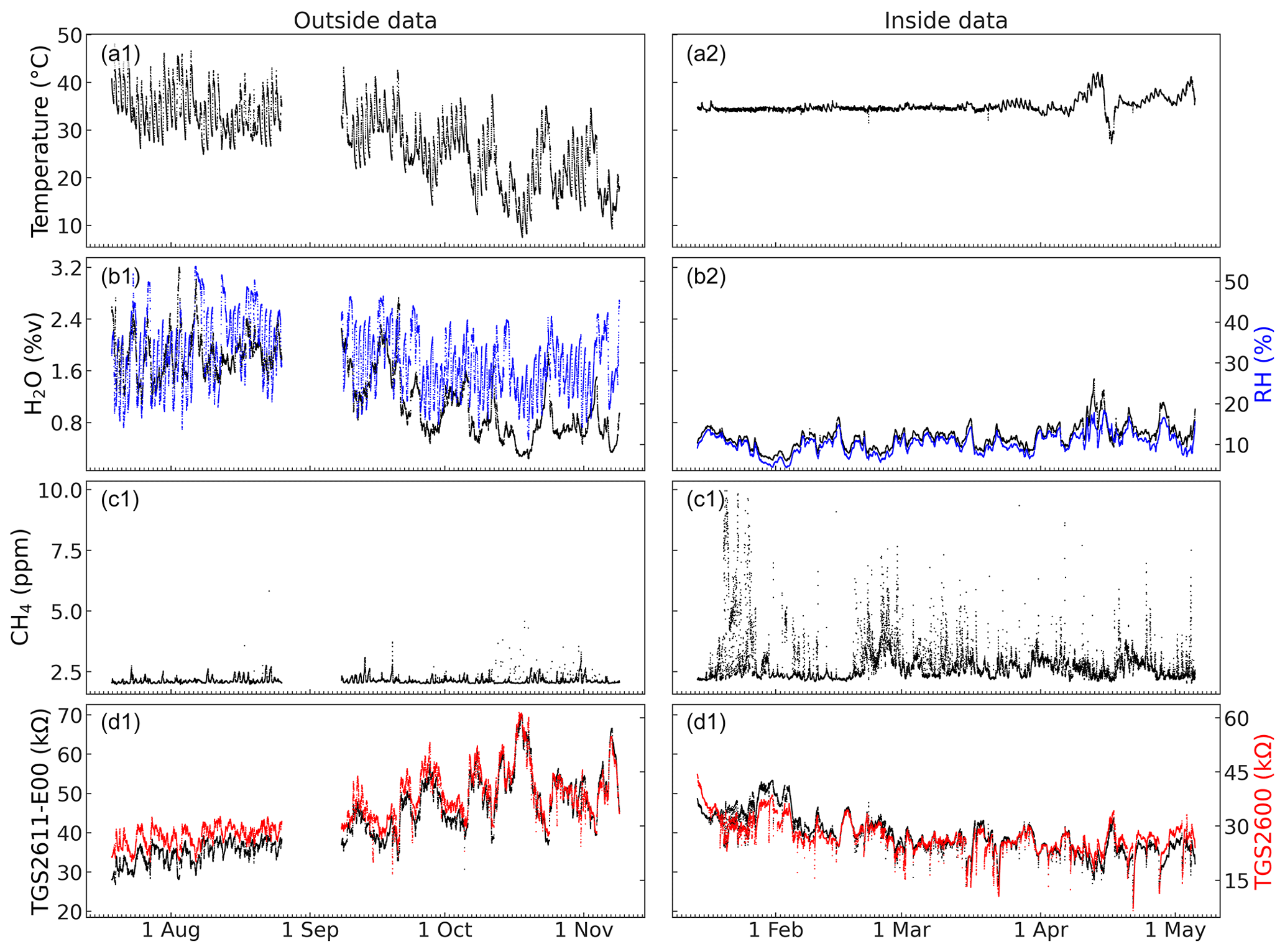
Figure 2 Time series of both experiments, with internal sensor node temperatures (a), water vapor concentration and relative humidity (b), methane data collected by the reference analyzer (c), and MOx sensor responses (d).

The outside experiment captured a range of temperatures and humidities over its 113 d span. The experiment began in summer, with associated high temperatures and water vapor concentrations; the end of the experiment was in autumn, with colder temperatures and lower water vapor levels. The temperature sensor was inside the system's enclosure, which experienced consistently higher temperatures than the outside air.

Some fluctuations in methane concentrations are visible in the outside dataset. We observed a diurnal cycle in methane levels with the reference analyzer for some periods of the experiment; we give an example of this cycle in Appendix C. Several unplanned sharp spikes occurred beyond our controlled releases, which may have been due to residential gas leaks or similar events.

The inside experiment ran for 111 d, beginning in winter and ending in spring. During winter, the location was heated to a relatively consistent temperature without added humidity. Accordingly, the temperatures were more stable than in the outside experiment, with overall lower water vapor levels and relative humidities. As with the outside sensor, the recorded temperatures were inside the sensor node enclosure, which was warmer than the ambient air.

Figure 3 shows data distributions and correlations between the different measured variables for the two portions of the experiment. In the outside experiment, the TGS2611-E00 and TGS2600 sensors were highly correlated (Pearson's r = 0.97), and both were strongly correlated with water vapor levels ($\left|r\right|$ > 0.8) and temperature ($\left|r\right|$ > 0.7). The sensors were not obviously correlated with methane levels ($\left|r\right|$ ≤ 0.14).

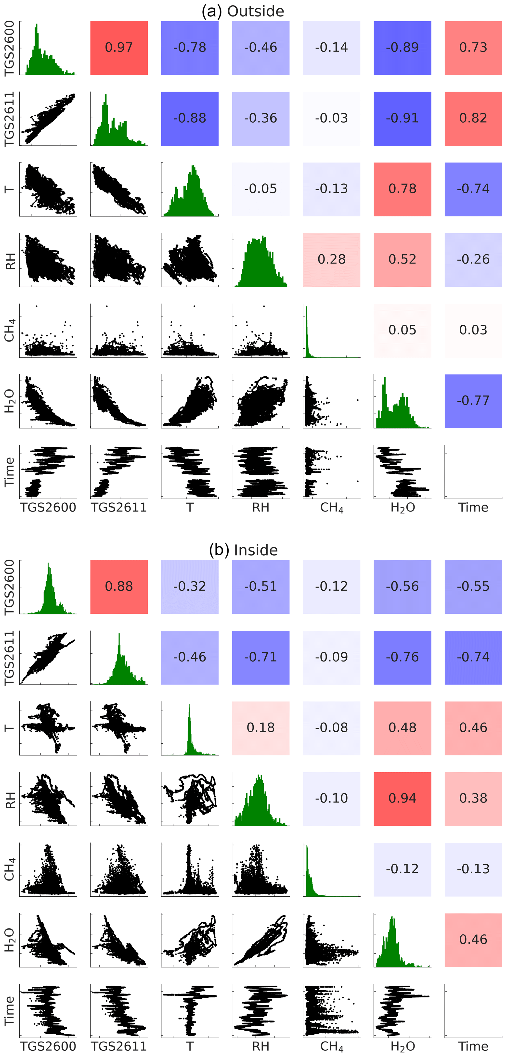
Figure 3 Correlations and data distributions for the outside (a) and inside (b) datasets. The upper triangle shows correlations (Pearson's r); the lower triangle shows pair plots between variables; the diagonal line shows histograms for each variable.

Sensor performance can be influenced by cumulative sensor run time in a variety of ways, which we will examine in more detail. We chose to capture this parameter as elapsed run time, representing the cumulative time the sensor had been powered on since the beginning of the outside experiment.

As seen in Fig. 3, sensor response was strongly correlated with elapsed time (r > 0.7) in both the inside and outside experiments. Due to seasonal changes, elapsed time was itself correlated with both water vapor concentrations and temperatures (which were themselves also correlated), as outdoor temperature and water vapor levels are higher in summer than in winter. Accordingly, it is possible that some portion of the sensor-time correlation was due to the well-known sensitivity to water vapor or due to an effect from temperature.

The MOx sensors were again strongly correlated with each other in the inside experiment (r = 0.88). Sensor correlation with water vapor concentrations ($\left|r\right|$ > 0.5) was stronger than with temperature ($\left|r\right|$ > 0.3), and the sensors were correlated moderately with elapsed time ($\left|r\right|$ > 0.5). Neither sensor showed a strong correlation with methane levels ($\left|r\right|$ ≤ 0.12).

3.2 Baseline sensor response

As described previously, we examined the baseline TGS2611-E00 response to environmental conditions. Our experiment recorded four parameters with potential effect on sensor response besides methane: temperature, water vapor concentration, relative humidity, and time. We used water vapor concentration and ignored relative humidity a priori based on our previous work (Furuta et al., 2022). Our first candidate baseline equation used these environmental factors to predict TGS2611-E00.

Our second candidate equation included a secondary sensor, TGS2600, which we have previously found not to respond to methane at low concentrations (Furuta et al., 2022); we hoped to remove the influence from non-target gasses and other unexpected factors by including TGS2600 in the baseline response. We selected all data with a measured methane concentration below 2.3 ppm, a value slightly above the background levels of approximately 2 ppm at our research locations, as the targets for our baseline regressions and compared the performance of the two baseline equations.

As previously described, we selected Eq. (1) as the best-performing regression without TGS2600. This regression closely fit the baseline TGS2611-E00 response, again defined as the sensor response for all datapoints with methane levels below 2.3 ppm. We obtained R² values of 0.97, 0.91, and 0.89 for the outside, inside, and combined datasets, respectively, and root mean square error (RMSE) values of 1.46, 1.56, and 2.81 kΩ, respectively.

The regressions capture the overall trend in the baseline response, as seen in Fig. 4a and c but with considerable variance. As shown by the color-coding, time appears to have an important effect on sensor response, supporting the inclusion of time in Eq. (1); for example, in the inside dataset in Fig. 4a, which had relatively little variation in humidity and temperature, the sensor shows a markedly different baseline response at different time periods of the experiment.

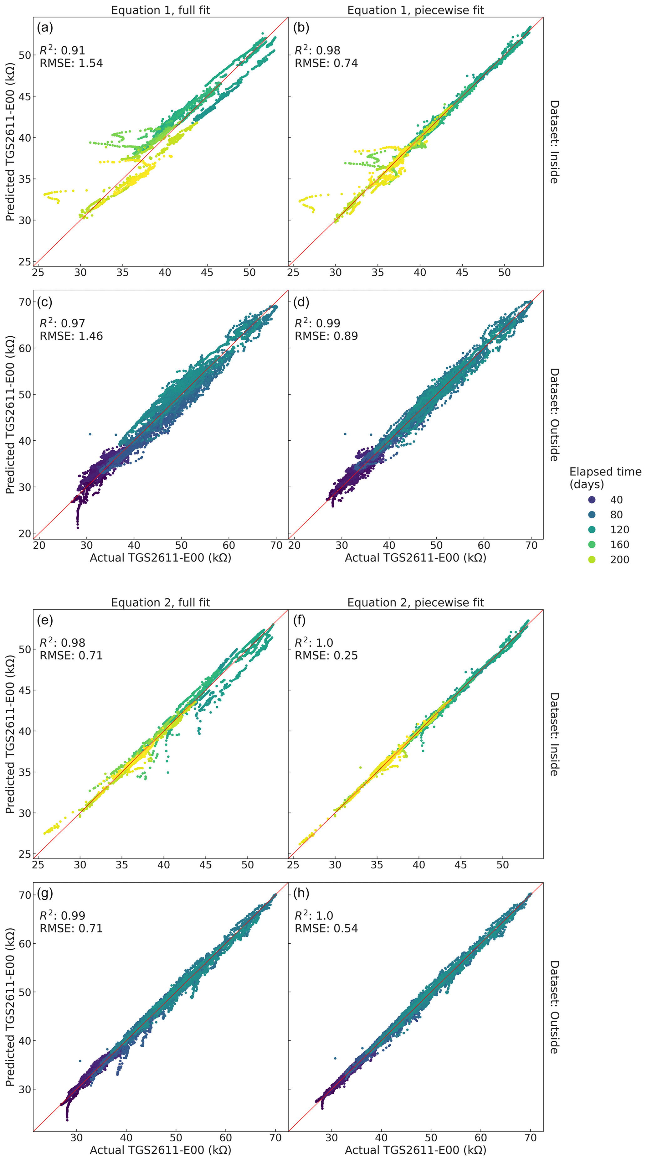
Figure 4 Results of TGS2611-E00 baseline regressions for the datasets, filtered to only include data below 2.3 ppm of methane, resulting in 3717 inside datapoints (a, b, e, f) and 13 030 outside datapoints (c, d, g, h). The system run time from the beginning of the outside experiment in days is coded as color. Panels (a)–(d) show the fit for Eq. (1), and panels (e)–(h) show those for Eq. (2), both with regressions over the full filtered datasets (a, c, e, g) and piecewise by time (b, d, f, h).

We then added the TGS2600 sensor response to the baseline equation as a potentially stronger regression. We have previously found that TGS2600 does not strongly respond to methane in the 10 ppm concentration range (Furuta et al., 2022). Accordingly, we hoped that the TGS2600 response would allow the baseline fit to accommodate unknown environmental effects, such as changes in ambient non-targeted gas concentrations, without affecting the relationship between the baseline fit and methane levels. Adding a term for TGS2600 produced Eq. (2), which we again fit for the low-methane data subsets.

Adding the TGS2600 term improved R² to 0.99, 0.98, and 0.98, and RMSE to 0.71, 0.73, and 1.21 kΩ for the inside, outside, and both datasets, respectively. As seen in Fig. 4e and g, the regressions still show some error, but the fit is closer than with Eq. (1), suggesting that Eq. (2) outperforms Eq. (1) for predicting the TGS2611-E00 baseline response.

Even with the additional sensor term, the accuracy of the regressions varies with time period, as can be seen in the coloring of Fig. 4. For example, the baseline at the beginning of the inside experiment in Fig. 4e has a worse fit than the baseline closer to the end of the experiment. To attempt to capture this change, we next examined a piecewise fit with respect to time for the baseline response. We divided the inside and outside subsets into 10 sections each, equally by number of datapoints, with each section corresponding to approximately 10 d (as the outside dataset has missing data, the sections are not all the same length of time). We then fit Eqs. (1) and (2) to each section and then collected the overall fits and evaluated RMSE and R².

The piecewise Eq. (1) approach resulted in R² of 0.98 and 0.99 and RMSE of 0.78 and 0.89 kΩ for the inside and outside subsets, respectively. The piecewise fit is better than the full-dataset approach, but some obvious issues are still visible, such as variation in the fit in Fig. 4b with later elapsed times.

The piecewise fit for Eq. (2) resulted in R² better than 0.99 for both sets, and RMSE of 0.30 and 0.54 kΩ for the inside and outside data, respectively. The piecewise Eq. (2) fit is the best quality of the options considered, with relatively minor error and a stronger fit than Eq. (1). For the inside dataset, the time variable was non-significant in 2 of the 10 piecewise subsets (p = 0.08 and 0.49), and the intercept was non-significant in one subset (p = 0.90); otherwise, all terms were significant in all subsets (p ≤ 0.001). Accordingly, we believe that including sensors to monitor non-target gasses and regularly recalibrating the baseline sensor response to capture changing environmental conditions will be helpful in deploying TGS2611-E00 and similar sensors.

As the piecewise Eq. (2) provided the best fit of the baseline regression candidates examined, we used it to produce the estimated baseline TGS2611-E00 response for our methane calibration.

3.3 Methane response

We examined the relationship between the sensor to baseline ratio and methane levels. As the inside dataset had a wider range of methane concentrations than did the outside set, we first fit only the inside data.

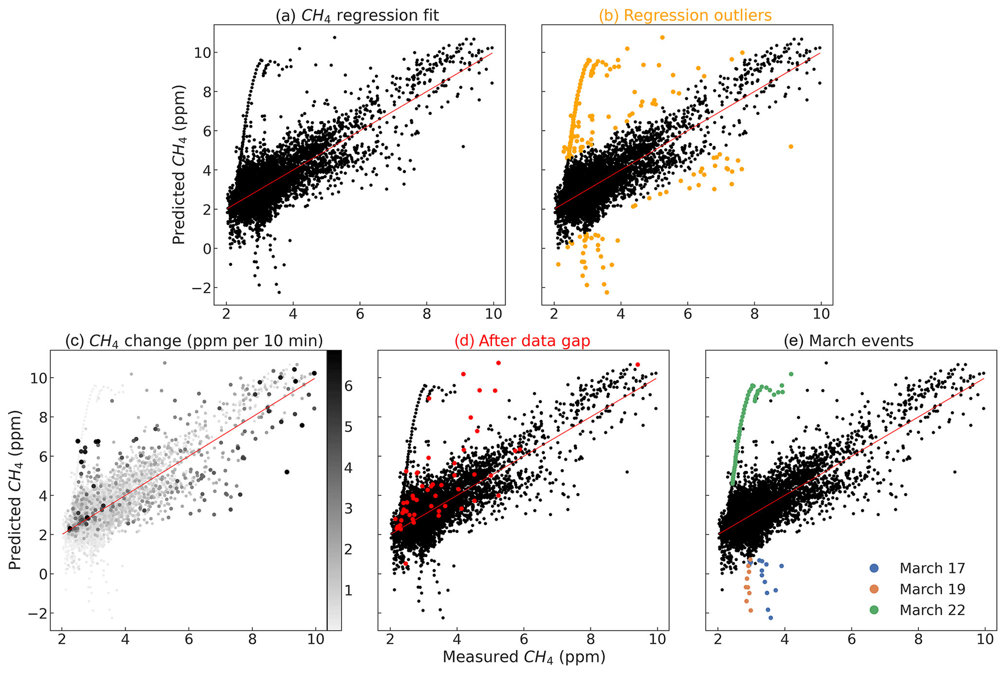
Figure 5 Methane fit results (a), 1 % outliers (b), points colored by rate of methane change (c), occurrence after a data gap (d), and the three events in March discussed in the text (e).

The TGS2611-E00 sensor response relative to the predicted baseline given by the piecewise Eq. (2) should be proportional to methane levels. Accordingly, we use Eq. (3) to estimate methane levels from the sensor response. We fit Eq. (3a) on the inside dataset, and then we rearrange the terms to produce Eq. (3b), which we evaluate for R² and RMSE. The fit on the inside dataset shows moderate performance, with R² = 0.46 and RMSE = 0.65 ppm. As seen in Fig. 5a, the fit is noisy but captures methane trends. The largest errors occur in the low concentration range, with the model both overpredicting and underpredicting some datapoints. The low concentration range is also overrepresented in the dataset. Despite this, the model does not have notable bias in either the lower or higher concentrations.

Our baseline regression used datapoints below 2.3 ppm of methane to produce a fit. If we evaluate the fit for methane only on datapoints above 2.3 ppm, excluding those used to produce the baseline, we find R² = 0.39 and RMSE = 0.58 ppm.

The 1 % of points with the worst fit, which we designate as outliers as highlighted in Fig. 5b, dominate the model error; neglecting these points, we find the reasonable performance of R² = 0.63 and RMSE = 0.53 ppm. Considering only the non-outlier points above 2.3 ppm of methane, we find R² = 0.58 and RMSE = 0.59 ppm. Some of the outlier data appear to have related trends, such as the group of overpredicted points in the upper left part of Fig. 5b. To better understand the cause of these errors and to understand possible difficulties for our model, we examined these outlier points. We found three main explanatory features of the outlier data.

First, as seen in Fig. 5c, we calculated the absolute change in methane concentration with the data immediately before and after each point, and we took the larger change of the two. Some of the outliers show a large rate of change; as our system is passive and relies on natural air movement and gas diffusion, it is possible that our sensor node did not respond to changes quickly enough to track the relatively rapidly shifting methane concentrations for these points. As previously mentioned, we analyzed the data as a series of 10 min averages: 40 % of the outliers show a rate of change greater than 1 ppm per 10 min; 31 % exceed 2 ppm per 10 min; and 6 % exceeded 5 ppm per 10 min. For the full dataset, 5.1 %, 1.7 %, and 0.16 % show the same rates of change, respectively, suggesting that the outliers are considerably more likely to occur during periods of rapidly changing concentrations.

Second, as noted previously, the methane concentrations exceeded the limits of our reference analyzer on several occasions. After each such spike, we removed 1 h of data to allow the systems to stabilize and resume normal functioning. We had additional gaps from occasional power failures or system downtime for data collection; 7 % of the outliers fell immediately after such data gaps, as compared to the 0.34 % of all points which occurred after a gap. Our calibration model tended to overpredict these points, as seen in Fig. 5d, suggesting that possibly our sensor node was still encountering a higher concentration in the sensing chamber than in the ambient air.

Finally, we found three runs of consecutive outlier points, highlighted in Fig. 5e – these periods each had a stretch of outlier points without breaks for one to several hours each. These three events showed patterns that appeared to be related, and so next we examine them in more depth. Together, these three events account for 45 % of the outliers.

The three explanatory categories had some overlap – some data from one of the anomalous events might have had a high rate of change, for example. In total, 87 % of the outliers either belonged to one of the three consecutive events, fell after a data gap, had a rate of change greater than 1 ppm per 10 min, or some combination.

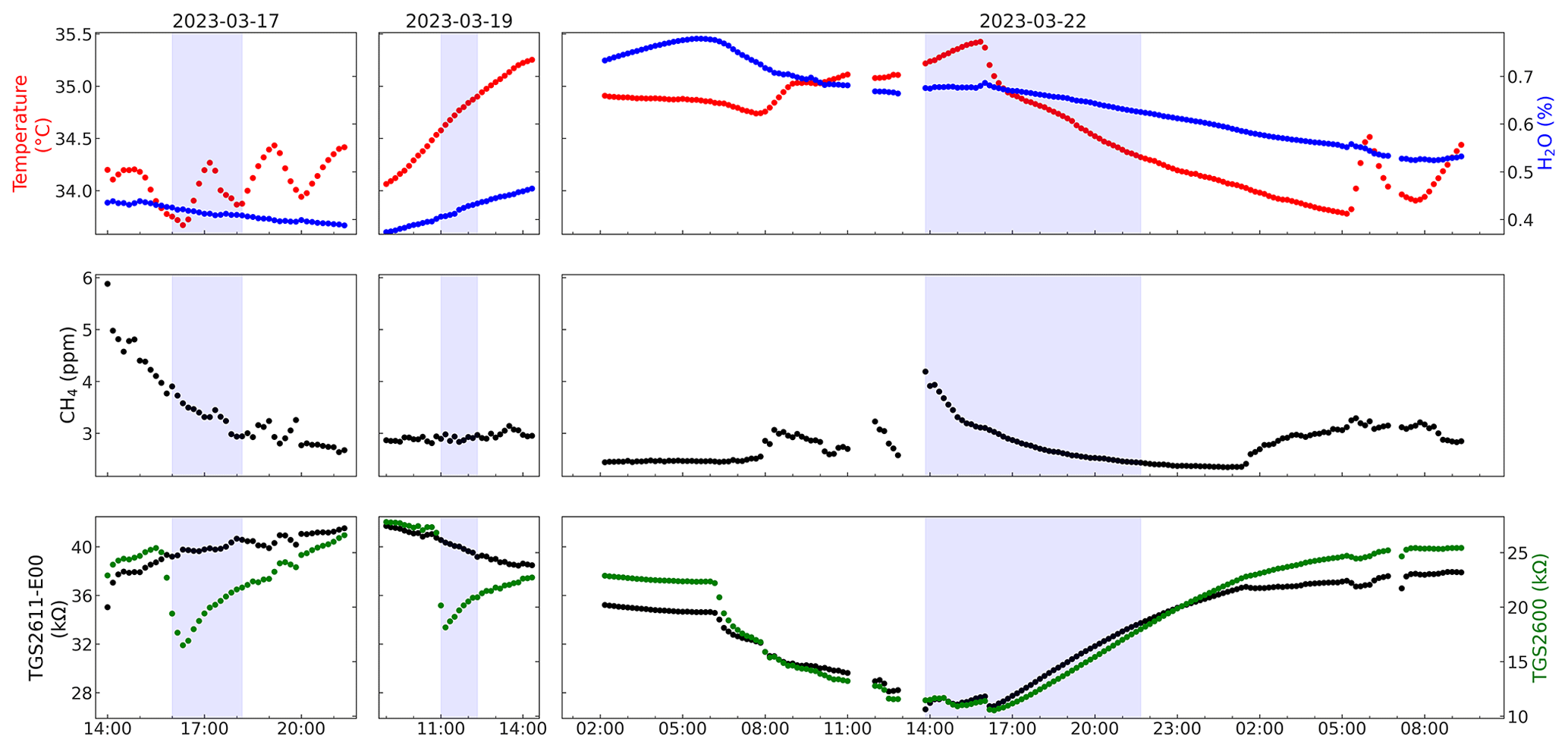
Figure 6 Time series plots of the three anomalous events. The light purple highlights represent consecutive periods of outlier points, as described in the main text.

Figure 6 plots the three consecutive outlier events. The first two events – on 17 and 19 March – show similar behaviors: in both cases the TGS2600 sensor exhibits a sharp and strong response to something other than methane or water vapor, without the TGS2611-E00 sensor responding. As the TGS2611-E00 has a filter to remove certain interfering gasses and the TGS2600 does not, we speculate that this response is likely the result of an unknown, non-target gas pulse. This strong signal causes an error in the baseline regression, leading to an erroneous methane prediction.

The third event, on 22 March, shows different behavior. Typically, the MOx sensors respond inversely to both water vapor levels and methane; in the depicted event, both sensors show an unexpected response through the day that is both stronger in magnitude and mostly in the opposite direction from the expected water vapor response. The sensor response is also much larger than we expected from the depicted methane fluctuations. We speculate, again, that the sensors were responding to some unknown gas, with a gradual release through the day and slow dissipation overnight.

Finally, we attempted the same approach on the outside dataset, fitting the baseline with the piecewise Eq. (2) and then predicting methane with Eq. (3b). As noted above, the baseline regression produced a strong fit, but the fit for methane did not capture any trend and failed to perform better than simply predicting the dataset mean; 97 % of the outside data had a methane concentration between 1.98 and 2.5 ppm, as compared with the 45 % of the inside data in the same range; as the RMSE for our inside methane model was greater than 0.5 ppm, the outside data appear to cover too small of a range to accurately fit.

The outside data cover a much wider temperature and water vapor range than the inside data, with substantial daily fluctuations. It is possible that fitting the baseline regression piecewise by temperature and water vapor would yield better results than by time, but as the baseline regression quality is already strong it is unlikely that a change in algorithm will produce acceptable performance in this small methane range.

3.4 Methane regression sensitivity to baseline fit

We fit the TGS2611-E00 baseline response with Eqs. (1) and (2), both over the full dataset and piecewise over time intervals – as a reminder, Eq. (2) included the TGS2600 sensor response as a term, while Eq. (1) did not. We derived the sensor methane response using the piecewise Eq. (2) baseline fit.

Figure 7 Sensor calibration results using the different baseline regression approaches.

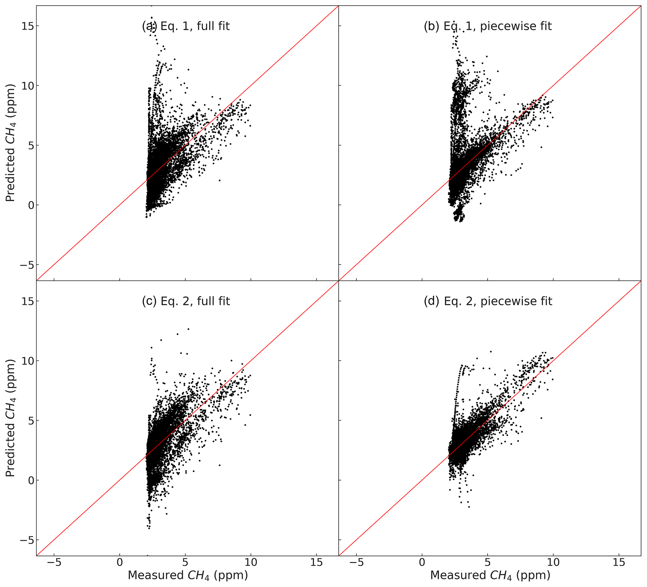
To examine whether this baseline fit is critical for sensor performance, we performed the methane calibration routine we described for the four possible baseline fits on the inside dataset, with results shown in Fig. 7. All of the regressions capture some trend in the methane response, but only the Eq. (2) piecewise fit (the approach we examined in detail previously) has positive R², indicating that predicting the dataset mean for each point would perform better than the other regressions; the other baseline equations lead to poor methane predictions in the low range, causing a poor overall fit. The methane fits using the full and piecewise Eq. (1) baseline produced R² values of −1.79 and −2.95 and RMSE values of 1.47 and 1.75 ppm, respectively, and the fit with the full Eq. (2) baseline produced an R² of −0.48 and RMSE of 1.07 ppm. Accordingly, it appears that tracking the changes in sensor baseline response to environmental conditions will be critical to successful field deployment.

4 Discussion

4.1 Sensor baseline determination and methane fit

We found that we could closely fit the baseline TGS2611-E00 response to environmental conditions at background methane levels. Water vapor, temperature, and sensor run time appear to largely determine the sensor baseline (R² > 0.9). The baseline fit performs better if approached piecewise with respect to time. The piecewise approach caused discontinuities between baseline predictions at the edge of adjacent calibration periods; a more sophisticated approach might interpolate regression parameters between calibration points, but we accepted the simple method as sufficient for this paper.

The sensor deviation from baseline showed a clear trend with methane levels, without notable bias, but with substantial uncertainty. The model appears adequate to capture substantial shifts in methane concentration, but it appears too noisy to monitor small changes. Our model can likely distinguish 2 ppm from 10 ppm, but appears unable to distinguish, for example, 2 ppm from 3 ppm. We speculate that some of the model's error is caused by changes in non-targeted ambient gas concentrations; previous studies have also noted this effect (Shah et al., 2023). We also believe that the passive nature of our sensor node may have caused a slower methane response than the active sampling reference analyzer, as seen in Appendix A; adding a pump to our sensor node would likely improve temporal resolution and reduce this lag or mismatch. Our sensor design showed excellent power supply stability and had good electrical resolution; accordingly, we think it is unlikely that the electronics contributed substantially to model error.

Our fit for methane as a function of sensor response showed moderate performance in the 2 to 10 ppm range we examined. Our calibration equation captured methane trends (neglecting outliers, R² = 0.63), but the previously mentioned difficulties and resulting outlier points led to compromised performance (with outliers, R² = 0.46). As the baseline fit was piecewise with respect to time, attaining this level of performance may require frequent recalibration of the sensor response to environmental factors.

We were similarly able to closely predict the baseline sensor response for our outside dataset, which predominantly had data close to background levels (2 ppm methane), but were not able to capture methane trends. We believe that this is likely a limitation of the sensors themselves, and that concentrations in the background to 2.5 ppm range, as encountered in our urban site, will be a poor application for this technology.

Various authors have claimed that TGS-series sensors require moderate relative humidity to operate consistently, with a threshold given of approximately 40 % (Eugster and Kling, 2012; van den Bossche et al., 2017; Riddick et al., 2022). Our inside dataset, with which we found moderate success in fitting sensor response to methane levels, had a maximum relative humidity of 18 % with a mean of 10 %; the low humidity levels were due to the large, heated, but not humidified study location in winter. As discussed previously, although humidity influences sensors' performance, it appears that unmonitored parameters other than humidity were also responsible for sensing difficulties; accordingly, it is not apparent that low humidity poses a fundamental problem for the application of TGS2611-E00 or similar sensors.

4.2 The importance of time

Some previous studies have found that different algorithms or parameters were required at different time periods, or that models developed in the lab demonstrated compromised performance in field experiments (Collier-Oxandale et al., 2018; Riddick et al., 2020; Shah et al., 2023). Some time-related factor, then, may be important for sensor response. Time was a significant parameter in our fit for sensor baseline response in two ways: first, including a parameter for elapsed sensor lifetime improved the model quality, and second, fitting the baseline piecewise over shorter time spans led to better performance.

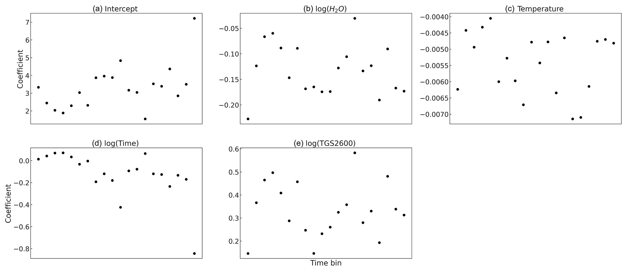
Figure 8 Best-fit regression coefficients for Eq. (2), fit across the combined dataset. As described in the text, the Time axis is not to scale. Panel (a) is the intercept; panels (b)–(d) are environmental parameters and time, and panel (e) is the non-methane responding MOx sensor.

To examine the nature of the piecewise fit, we fit Eq. (2) over the full dataset (both outside and inside) split into 20 sections. The time chunks for the piecewise fit are not necessarily of equal temporal length due to gaps in the data but instead each contain the same number of datapoints. As seen in Fig. 8, the best-fit regression coefficients change in a non-monotonic manner, although with some apparent visible patterns.

We speculate that the change in best-fit parameters for the sensor baseline over time is due to changing environmental parameters that our setup was unable to measure, such as interfering gasses or ambient air makeup; sensor aging may play a role as well, but as the coefficients change in a non-monotonic manner aging may not be a primary cause.

We suggest that previous difficulties implementing these sensors may have resulted from similar issues. Determining whether other ambient gasses, sensor aging, or other factors are responsible will require further investigation. We believe this underlying issue is the next problem to address for the practical use of these sensors for methane monitoring, and that deployment in more extensive sensor arrays targeting different gasses will improve methane monitoring results.

4.3 TGS2600 performance for methane sensing

Some previous studies have used TGS2600 to monitor methane levels. We repeated our analysis, exchanging TGS2600 and TGS2611-E00 in Eqs. (1) and (2) for the background fit, and then again attempting to fit methane response as a function of the TGS2600 to background fit ratio.

We found that we could closely fit the sensor baseline response, with R² of 0.98 and RMSE of 0.73 kΩ for the modified piecewise Eq. (2), closely comparable to the values of 0.99 and 0.71 kΩ for TGS2611-E00. For the modified piecewise Eq. (1), we found R² of 0.91 and RMSE of 1.53 kΩ. However, both possible fits (with the Eq. 1 or Eq. 2 baselines) for methane had negative R² values (−29.0 and −26.9 for the fits using Eqs. 1 and 2, respectively), indicating that simply predicting the data mean would perform better. Both fits had RMSE worse than 4.5 ppm. This result is consistent with our previous work showing little to no response from TGS2600 in the 2 to 10 ppm concentration range (Furuta et al., 2022). Accordingly, we believe that TGS2600 does not have promise for methane sensing in the near-background concentration range.

The inability of TGS2600 to sense low concentrations of methane may be beneficial if it is included in a sensor array with TGS2611-E00 and other sensors; possibly, such a sensor array could reduce any effect of non-target gas species, and give greater insight into gas compositions than possible with a single sensor.

5 Conclusions

Our sensor node demonstrates the feasibility of a low-cost, high-performance implementation of the TGS2611-E00 or similar MOx sensors. Our system design provided stable operating conditions for the MOx sensors for over half a year of field tests and could be powered by an inexpensive battery and solar panel in a stand-alone deployment. Our unit had a parts cost of under USD 200; future revisions could easily reduce costs further by implementing the data logger and telemetry from components rather than using off-the-shelf microcontroller modules.

We found TGS2611-E00 to respond to methane, consistent with our previous work (Furuta et al., 2022). Contrary to some previous studies but consistent with our previous work, we did not find TGS2600 to respond to methane in the studied 2 to 10 ppm range using the algorithms we examined.

Our results suggest that similar sensor networks may be worth investigating for applications with wider methane concentrations of interest than our 2 to 10 ppm range, such as around landfills, animal agriculture and manure processing, wastewater treatment, fossil fuel infrastructure, or other near-source settings. Our sensor response correlates with methane levels with moderate accuracy (RMSE < 0.6 ppm) in the 2 to 10 ppm range, but caution is necessary to account for environmental factors. Our system was unable to capture methane trends in the 2 to 3 ppm range in our outdoor test, which featured both lower methane levels and wider humidity and temperature variation than our indoor setting. This variation will be typical in outdoor deployments in many climates and poses challenges for the sensors.

In addition to MOx sensors' well-known sensitivity to water vapor levels, we found that sensor performance varied over time, possibly in response to changing ambient gas compositions, sensor aging, or other unmeasured environmental changes. We believe that this sensitivity will limit the ability of these or similar sensors to accurately monitor low methane concentrations in many real-world settings without further work to detect and correct for other gasses or environmental factors. We believe that this behavior may ultimately determine the lower limit for practical deployment of these sensors as standalone units.

Our results could possibly be improved by filtering or monitoring and accounting for interfering gasses. Converting our system to active sampling with the addition of a pump could also help reduce the system's lag time, and might allow the unit to capture sharper methane peaks. Even with these improvements, it is likely that these MOx sensors will be better suited to methane concentrations above the 2 to 10 ppm range we examined.

Appendix A: Sensor node electronic design, startup behavior, and lag

A1 Sensor node design

Our sensor node consists of two circuit boards: a main controller board and a sensor board. The two boards are connected via a cable. The main board is responsible for telemetry, data storage, and system control; the sensor board allows for up to two Figaro MOx sensors, a relative humidity and temperature sensor, and power regulation for the Figaro sensors. The full device is pictured in Fig. 1a of the main text.

Figure A1 Schematic for the sensor circuit board.

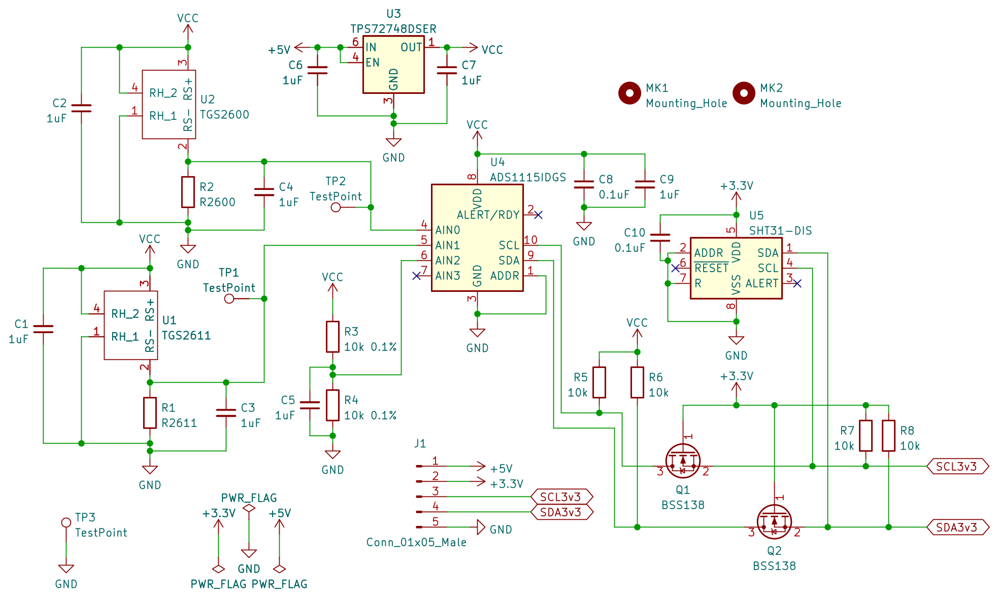
Figure A1 shows the sensor circuit board. Digital communication between the controller and sensor boards is provided via I²C with a high voltage of 3.3 V. The Figaro MOx sensors are specified with a 5 ± 0.2 V supply (Figaro USA, Inc., 2013, 2022b). We provide a 5 V supply from the controller board; however, as power supply stability is critical to accurate sensor readings, we further regulate the supply with component U3, a precision voltage regulator with a fixed 4.8 V output. As discussed in the main text, this arrangement proved stable over the course of the experiment.

The MOx sensors U1 and U2 are implemented in voltage divider configurations with R1 and R2, which were chosen to approximately match the expected sensor resistances, as discussed in the main text. The output voltages from the dividers are digitized by U4, a 16-bit ADC. We also digitize the 4.8 V supply through R3 and R4, allowing us to correct for any drift and to evaluate the regulator performance. U4 contains an internal precision voltage reference. The ADS1115 has a resolution of 188 µV, corresponding to a resolution of 12 Ω against the 75 kΩ reference resistor and 2.3 Ω against the 15 kΩ reference resistor when the sensor resistances equal the references.

We sense temperature and relative humidity using U5, an integrated, digital-output chip. U4 and U5 communicate with the controller board via I²C; as U4 is operating at 4.8 V, level shifting is required for communication with the 3.3 V controller device. We provide level shifting via Q1, Q2, and the associated pull-up resistors R7 and R8.

All capacitors on the board are provided for power supply bypassing to reduce noise and instability, and all were X7R dielectric ceramic capacitors.

Figure A2 Schematic for the main board.

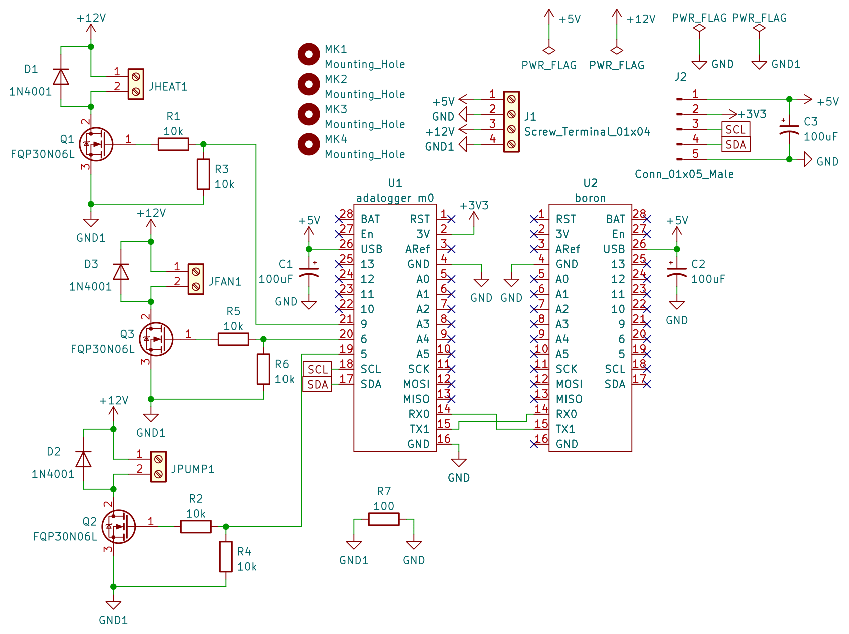
Figure A2 provides the schematic for the main board. U1 is a complete microcontroller module, including a processor, 3.3 V power regulator, SD card socket for data storage, and supporting circuitry. We use U1 as the main controller for the whole system, as well as for data storage. U2 is a microcontroller module with a cellular modem; we only use this board for telemetry and as a networked clock. We only used the telemetry data to remotely check that the system was operating correctly, and our analysis used the locally stored 5 s scale data.

Q1 through Q3 and their supporting components are provided to optionally drive a fan, pump, heater, or other similar devices; we did not use these components for the current experiment, and we left them unpopulated on the circuit board. As with the sensor board, we placed capacitors C1 through C3 to bypass the power supply for lower noise and greater stability; all three were aluminum electrolytic capacitors.

Figure A3 Circuit layout for the sensor board.

Figure A4 Controller board layout.

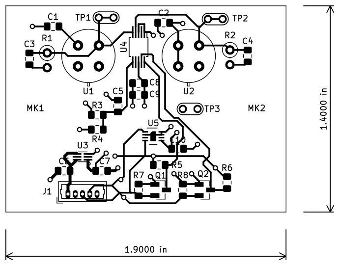
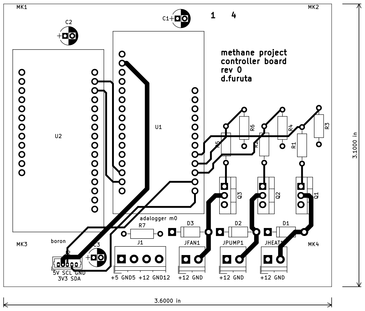
Figures A3 and A4 show the board layouts. Both boards are four-layer stacks. For clarity, the inner two layers containing ground and power planes have been omitted from the figures. We are aware of one mistake on the board layout: J1 on the sensor board should be reversed. For our prototype unit, we simply reversed the cable connection to this part. As mentioned previously, the fan, pump, and heat components on the main board were not used or populated for this experiment but are provided in the layout for future development. We hand-soldered and assembled the boards for this experiment.

A2 System startup behavior

Figure A5 shows the startup behavior of the system for the first 5 h of each time the system was powered up over the course of the experiment, including both the indoor and outdoor sections. In most of the cases, the system appears to have fully stabilized relatively quickly, with an initial warmup curve of a less than half an hour.

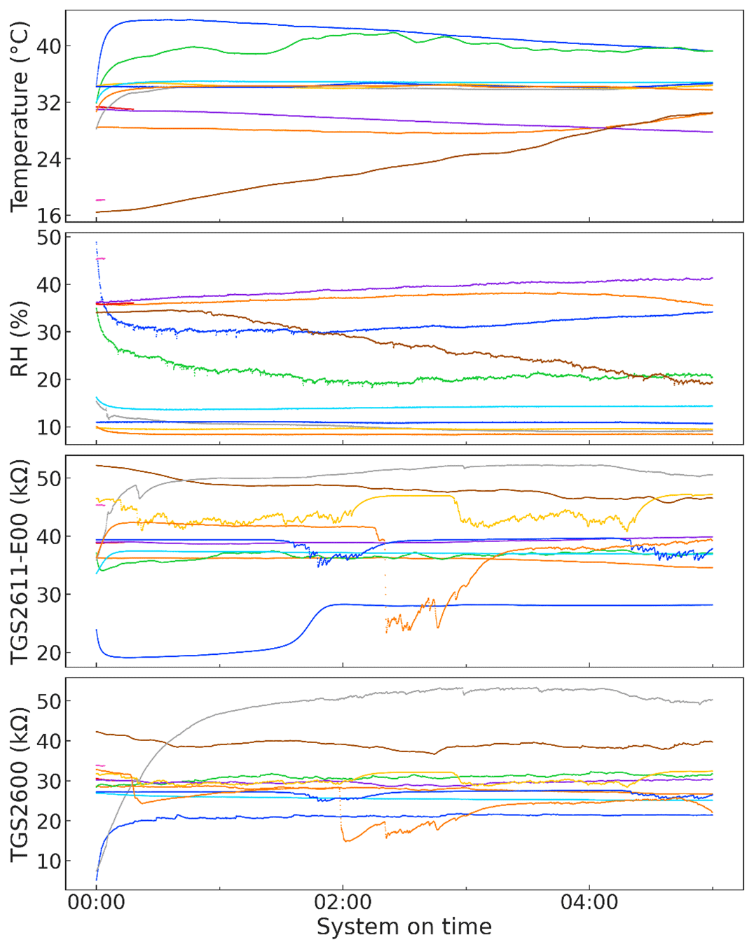
Figure A5 System behavior for every time the device was powered on over the course of the experiment. Each startup incident is color-coded consistently between the panels.

A3 Sensor lag

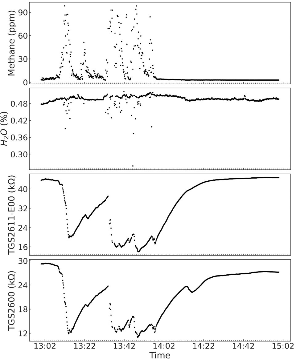
As discussed in the main text, our sensor node operates passively, without a pump, and accordingly has some lag in its response. To illustrate this effect, Fig. A6 shows raw sensor data collected around a series of large methane spikes in the indoor portion of our experiment, along with methane and water vapor data collected by the reference analyzer. The sensor node responds quickly to the spike's enhancement, but takes longer to return to baseline after the spike has passed.

Figure A6 Raw data around a series of large methane spikes, illustrating the sensor lag.

Appendix B: Baseline regression equation selection

As discussed in the main text, we examined different possible regressions to fit the TGS2611-E00 response to baseline environmental conditions other than methane. We fit the regressions on the datasets filtered to only include points with methane concentrations less than 2.3 ppm, which we assumed would be too small of an enhancement over the 2 ppm background for the sensor to respond. For the inside dataset, 3717 of the 15657 points were below the 2.3 ppm threshold, and for the outside dataset 13 030 of the 14 330 points were included.

Table B1 The three best-performing baseline regressions for each dataset with or without TGS2600 as a term, sorted within each category by RMSE.

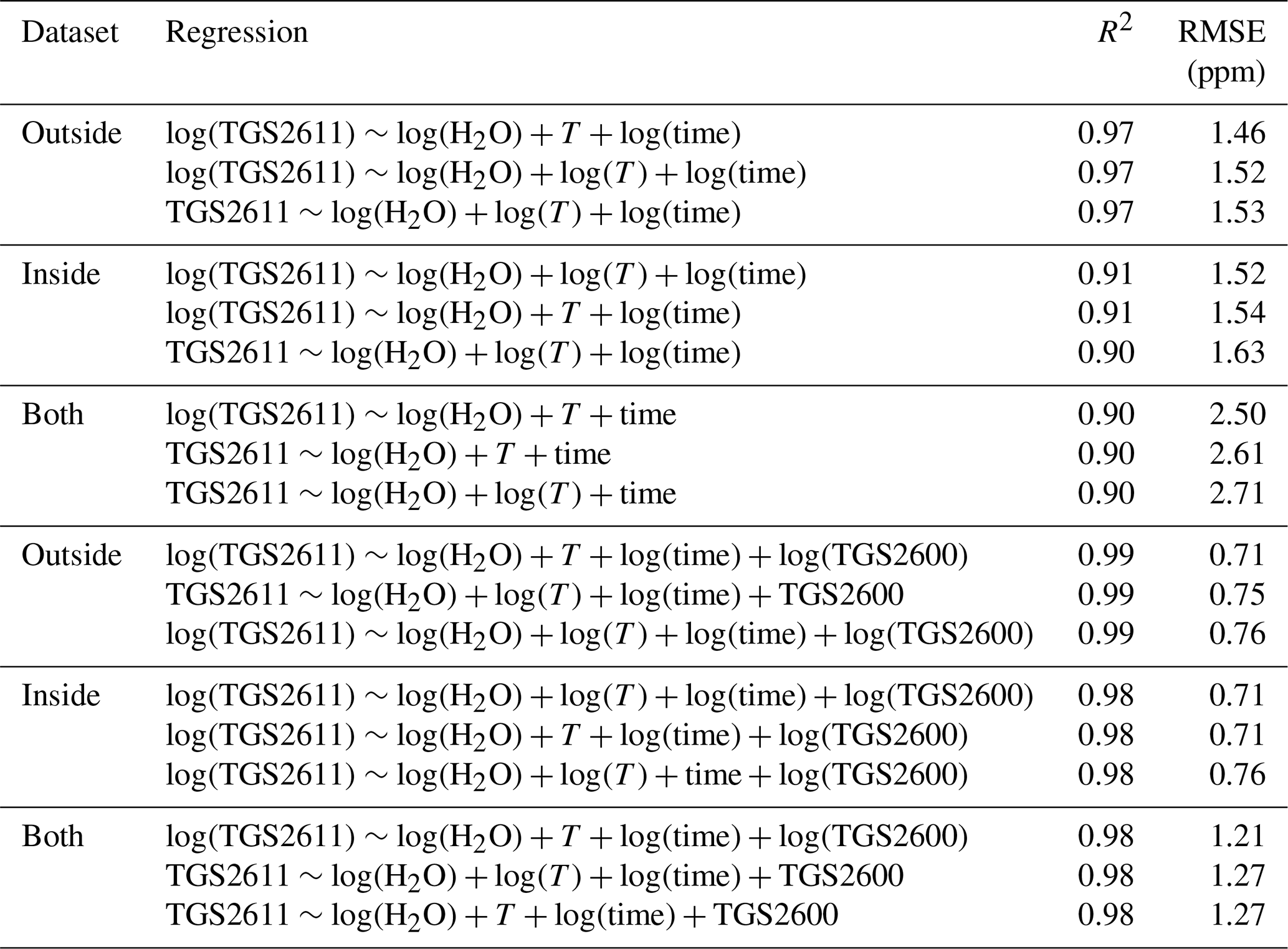
As explained in more detail in the main text, we have four possible factors for the TGS2611-E00 baseline regression: water vapor concentration, temperature, elapsed sensor run time, and TGS2600 response. We also examined factors transformed by the natural log, chosen as a standard regression transformation; we adjusted the log-transformed time variable by a negligible amount to account for zero values. We fit all regressions possible from Eq. (B1) on the inside data and outside data, and both sets together. As our regression results, shown in the main text, did not show clear bias in their residuals, we did not consider further transformations beyond the log.

$$\begin{array}{}\text{(B1)}& y=\mathit{\alpha }+{\mathit{\beta }}_{\mathrm{1}}{x}_{\mathrm{1}}+{\mathit{\beta }}_{\mathrm{2}}{x}_{\mathrm{2}}+{\mathit{\beta }}_{\mathrm{3}}{x}_{\mathrm{3}}+{\mathit{\beta }}_{\mathrm{4}}{x}_{\mathrm{4}},\end{array}$$

where $y\in \mathit{\{}\mathrm{TGS}\mathrm{2611},\log (\mathrm{TGS}\mathrm{2611}\left)\mathit{\right\}}$, $x_{\mathrm{1}}\in \mathit{\{}{\mathrm{H}}_{\mathrm{2}}\mathrm{O},\log ({\mathrm{H}}_{\mathrm{2}}\mathrm{O}\left)\mathit{\right\}}$, $x_{\mathrm{2}}\in \mathit{\{}T,\log (T\left)\mathit{\right\}}$, $x_{\mathrm{3}}\in \mathit{\{}\mathrm{time},\log (\mathrm{time}+\mathrm{0.0001}\left)\mathit{\right\}}$, and $x_{\mathrm{4}}\in \mathit{\{}\mathrm{TGS}\mathrm{2600},\log (\mathrm{TGS}\mathrm{2600}\left)\mathit{\right\}}$. We evaluated each regression for R² and RMSE. Regressions using the log-transformed TGS2611-E00 response as the target were transformed back to linear space prior to evaluating performance. We show the performance of the three best regressions on each dataset without TGS2600 and the three best with TGS2600 (equivalent to β₄ in Eq. B1 taking a zero or non-zero value, respectively) for each dataset in Table B1, chosen by lowest RMSE. The regressions are shown in shorthand; for example, $\log \left(\mathrm{TGS}\mathrm{2611}\right)\sim \log \left({\mathrm{H}}_{\mathrm{2}}\mathrm{O}\right)+T+\log \left(\mathrm{time}\right)$ is shorthand for the regression equation $\log \left(\mathrm{TGS}\mathrm{2611}\right)=\mathit{\alpha }+{\mathit{\beta }}_{\mathrm{1}}\log \left({\mathrm{H}}_{\mathrm{2}}\mathrm{O}\right)+{\mathit{\beta }}_{\mathrm{2}}T+{\mathit{\beta }}_{\mathrm{3}}\log (\mathrm{time}+\mathrm{0.0001})$.

As seen in Table B1, several equations occur repeatedly; in particular, the top three equations without TGS2600 are the same for the inside and outside datasets, in different orders but with similar RMSE and R² values. As $\log \left(\mathrm{TGS}\mathrm{2611}\right)\sim \log \left({\mathrm{H}}_{\mathrm{2}}\mathrm{O}\right)+T+\log \left(\mathrm{time}\right)$ performs well for both the inside and outside datasets and as it performs best across the datasets with the added log (TGS2600) term, we chose this regression to use as our Eq. (1) in the main text and the version with added log (TGS2600) to use as Eq. (2).

Appendix C: Diurnal patterns in methane levels

We observed diurnal patterns in methane levels in some portions of the outside dataset, as seen in Fig. C1c1, with increases in methane levels at night and lower levels in the day. The time period depicted was a rainy week; diurnal patterns were smaller or absent in dry periods.

Methane levels at our inside site also fluctuated, as seen in Fig. C1c2. These fluctuations appeared to be primarily the result of interactions with the anaerobic digester, with pulses occurring when the digester was opened for feeding or gas removal. The digester also likely released methane sporadically when internal pressure was released through its pressure relief system, which was simply a tube submerged in several inches of water.

Figure C1 Examples of short periods of the outside (a1–d1) and inside (a2–d2) experiments.