Investigation of gravity waves using measurements from a sodium temperature/wind lidar operated in multi-direction mode

A narrow-band sodium lidar provides high temporal and vertical resolution observations of sodium density, atmospheric temperature, and wind that facilitate the investigation of atmospheric waves in the mesosphere and lower thermosphere (80–105 km). In order to retrieve full vector winds, such a lidar is usually configured in a multi-direction observing mode, with laser beams pointing to the zenith and several off-zenith directions. Gravity wave events were observed by such a lidar system from 06:30 to 11:00 UT on 14 January 2002 at Maui, Hawaii (20.7° N, 156.3° W). A novel method based on cross-spectrum was proposed to derive the horizontal wave information from the phase shifts among measurements in different directions. At least two wave packets were identified using this method: one with a period of ∼ 1.6 h, a horizontal wavelength of ∼ 438 km, and propagating toward the southwest; and the other one with a ∼ 3.2 h period, a ∼ 934 km horizontal wavelength, and propagating toward the northwest. The background atmosphere states were also fully measured and all intrinsic wave properties of the wave packets were derived. Dispersion and polarization relations were used to diagnose wave propagation and dissipation. It was revealed that both wave packets propagate through multiple thin evanescent layers and are possibly partially reflected but still get a good portion of energy to penetrate higher altitudes. A sensitivity study demonstrates the capability of this method in detecting medium-scale and medium-frequency gravity waves. With continuous and high-quality measurements from similar lidar systems worldwide, this method can be utilized to detect and study the characteristics of gravity waves of specific spatiotemporal scales.

1 Introduction

Atmospheric gravity waves are generated when air parcels are perturbed vertically, and gravity or buoyancy acts as the restoring force. They can propagate vertically up to the thermosphere and horizontally over a considerable distance (up to several thousand kilometers). The most common wave sources include convection, orography, and fronts, among others (Fritts and Alexander, 2003, and references therein). The momentum and energy transported by gravity waves dramatically impact the general circulation and thermal structure of the middle and upper atmosphere. Phenomena and processes include, but are not limited to, the cold summer mesopause (Holton, 1982; Siskind et al., 2012), the quasi-biennial oscillation (QBO) in the tropical lower stratosphere (Ern et al., 2014) and the semiannual oscillation (SAO) in the upper stratosphere/lower mesosphere (Ern et al., 2015), instability and turbulent mixing in the atmosphere (Fritts, 1984; Fritts et al., 2013), as well as irregularities and traveling ionospheric disturbances (Fritts and Lund, 2011; Liu and Vadas, 2013), which are all related to gravity waves. Therefore, understanding gravity wave generation, propagation, and breaking has significant impacts on weather and climate applications.

Theoretically, gravity waves are governed by the fluid Euler equations for a set of fundamental variables including pressure p, density ρ, temperature T, and zonal, meridional and vertical winds (u, v, w). Many theoretical and observational studies of gravity waves are based on the linear wave theory, and it is commonly used to quantify the propagation and dissipation characteristics of gravity waves. The linearization of the Euler equations is implemented under different assumptions regarding wave and background atmosphere properties. Except for waves with very large horizontal scales, the effect of earth's rotation is often ignored. Zhou and Morton (2007) derived the Euler equations for a compressible atmosphere with altitude-varying background temperature and wind. Taylor (1931) and Goldstein (1931) derived the 2-D Euler equations with the Boussinesq approximation in a continuous shear flow without temperature variations. These specific Euler equations are referred to as Taylor–Goldstein equations (Nappo, 2012). Fritts and Alexander (2003) derived the Euler equations without wind shear but considered the Coriolis effect. Linearized wave solutions require that the vertical wavenumber m be independent of altitude. Strict independence is not likely since background temperature and wind vary with altitude. If the variations are relatively slow within the range of the vertical wavelength, the Wentzel–Kramer–Brillouin (WKB) approximation is applied. A monochromatic gravity wave can be assumed to be a traveling plane wave and represented by a sinusoidal function in the form of

$$\begin{array}{}\text{(1)}& \begin{array}{rl}& W(x,y,z,t)=\\ & A\cdot \exp \left[i(kx+ly+mz-\mathit{\omega }t+\mathit{\varphi })+{\displaystyle \frac{z}{\mathrm{2}{H}_{\mathrm{s}}}}\right],\end{array}\end{array}$$

of which x, y, and z are zonal, meridional, and vertical distances in a local Cartesian coordinate, and k, l, and m are zonal, meridional, and vertical wavenumbers. ω and ϕ are the observed (Eulerian) angular wave frequency and initial phase, H_s is the atmospheric density scale height, and $\mathrm{1}/\left(\mathrm{2}{H}_{\mathrm{s}}\right)$ corresponds to the wave amplitude growth rate with increasing altitude for upward propagating gravity waves without dissipation.

Many remote-sensing and in situ techniques have been developed to observe atmospheric gravity waves and their influences in past decades. There is an inherent “observation filter” (Alexander, 1998; Gardner and Taylor, 1998; Alexander et al., 2010) in any of these observation instruments such that they can only measure part of the gravity wave spectrum. Single-site ground-based techniques like lidar (Hu et al., 2002; Li et al., 2007; Lu et al., 2009; Cai et al., 2014; Chen et al., 2016), radar (Nastrom and Eaton, 2006; Fritts et al., 2010; Liu et al., 2013), and space-based limb-sounding satellites (Jiang et al., 2005; Alexander et al., 2009) are limited to providing vertical profiles and can only resolve vertical structures of the wave field. Other techniques like nadir sounding satellites (Gong et al., 2012; Alexander and Grimsdell, 2013; Hoffmann et al., 2014) and airglow imaging (Taylor, 1997; Espy et al., 2006; Li et al., 2011; Fritts et al., 2014; Cao and Liu, 2022) can only retrieve the horizontal structures over a certain area. In some cases, the unobserved horizontal or vertical information can be estimated by indirect methods based on the polarization and dispersion relationships (Hu et al., 2002; Lu et al., 2015). For reliable estimates of intrinsic wave parameters and characterization of the dissipation process, it is necessary to observe gravity waves fully in both horizontal and vertical directions, i.e., in 3-D space. Measurements from multiple complementary instruments, such as co-located lidar and the airglow imager, provide good opportunities to resolve gravity waves in both vertical and horizontal directions (Bossert et al., 2014; Lu et al., 2015; Cao et al., 2016). More space-borne limb-sounding observations were also analyzed with special techniques to resolve the gravity wave as fully as possible. Two-dimensional (2-D) limb-sounding measurements along a single satellite track, such as temperature variations from the High-Resolution Dynamics Limb Sounder (HIRDLS), were used to estimate the horizontal wavelength and momentum flux for individual wave events (Alexander et al., 2008). However, there were considerable uncertainties in the derived wave properties because the 2-D sampling measures only the apparent wavelength, which is likely longer than the actual one. This was also illustrated by combining rarely occurring co-locations of two HIRDLS profiles and one COSMIC radio occultation (RO) profile (Alexander et al., 2015), which showed that the 2-D method overestimated the occurrence of long horizontal wavelength waves relative to the 3-D method and underestimated momentum flux. Multiple methods have been proposed to resolve the intrinsic horizontal propagation and momentum flux assuming a dominant wave mode within a spatial (latitude and longitude) and temporal window large enough that it is coherent across more than three RO profiles (Wang and Alexander, 2010; Faber et al., 2013). Several studies have analyzed the horizontal wave information from closely spaced profiles in serendipitous geometries, for example, from COSMIC satellites just after launch and before they have separated into their final orbits. Alexander et al. (2018) used four spatially and temporally close RO profiles to derive intrinsic wave propagation and wavelength. These previous studies demonstrate the challenges and importance of resolving gravity waves as fully as possible.

The measurement profiles retrieved from narrow-band sodium lidar systems were typically used to observe the temporal and vertical variations of the gravity waves. This study provides a prospective solution to partly address the “observation filter” effect of these lidars by resolving often neglected horizontal wave information. We propose a novel method using cross-spectrum to retrieve the slight phase shift among the measurements from different laser beams and derive the horizontal wave information. Temperature and wind measurements on the night of 14 January 2002 from a lidar deployed in the Maui/Mesosphere and Lower Thermosphere (Maui/MALT) campaign are used to demonstrate the proposed method. The paper is organized as follows: Sect. 2 describes the instrumentation and methodology. Section 3 presents the observational results and diagnostic analysis. Section 4 presents a sensitivity study to demonstrate the capability of this method. Finally, the discussions and summary are presented in Sect. 5. Extra figures are included in the Appendix as supporting information.

2 Instrumentation and methodology

A narrow-band sodium lidar measures the atmospheric temperature and wind in the mesopause region (80–105 km) based on the thermal broadening and Doppler shift of atomic spectral lines of the sodium atoms. The sodium lidar transmits pulsed laser tuned to the sodium D2a line at 589.158 nm into the sky and the fluorescence scattered photons are collected by optical telescopes. The temperature and line-of-sight (LOS) winds are retrieved based on the well-known shape of the Na atomic spectrum using a three-frequency technique (She and Yu, 1994; Krueger et al., 2015). In order to measure the full 3-D wind vectors, the laser beam is configured to point to multiple directions, at zenith and off-zenith at several cardinal directions. A sodium lidar system operated by the University of Illinois at Urbana-Champaign (UIUC) was deployed at Air Force Maui Optical Station (AMOS) at Maui, HI (20.7° N, 156.4° W) from January 2002 to June 2007 (Liu, 2023). The laser transmitter was fixed, but the laser beam was directed by multiple mirrors to point to five directions: zenith (Z), 30° off zenith to the north (N), south (S), east (E), and west (W). The laser beam has an average output power of 1 W at 30 pps (pulses per second). A steerable astronomical telescope of 3.67 m diameter was coupled with the laser beam. The return photons were collected by the telescope pointing in the same direction as the laser beam. Figure 1a shows the orientation of laser beams in five directions. With a 30° off-zenith angle, there is a ∼ 50 km separation distance between the off-zenith and zenith directions at 90 km altitude. The laser beam was directed to rotate in a Z–N–E–Z–S–W sequence and the photon integration time was 1.5 min at each direction with a 1.7 min cadence (extra ∼ 0.2 min for telescope steering). The resulting measurement intervals at zenith and any off-zenith directions were 5.1 and 10.2 min; however, some irregularities existed because of mechanical issues. In order to accommodate the data processing of filtering and spectral analysis, the raw data of all directions was interpolated into the regular 6 min interval. The targeted waves presented in this study have much longer periods and interpolation would not yield any artifacts. An example of the time series of the temperature perturbations of one target wave without interpolation is shown in Fig. A3. The spatial resolution of measurements is 500 m along the laser beam in all directions. The temperature and winds from off-zenith directions are interpolated to the same altitude grids as the Z direction with a uniform 500 m resolution. The lidar-measured temperature and wind accuracies largely depend on the sodium atom density; thus, they vary with altitudes. With the temporal and spatial resolutions in this study, the accuracies are ∼ 2 K for temperature and ∼ 4 m s⁻¹ for horizontal winds near the peak sodium density altitudes (Li et al., 2012; Krueger et al., 2015). The most reliable measurements are mainly within the 85–105 km altitude. The mean sodium atom density and the altitude-varying accuracies for temperature as well as horizontal and vertical winds are given in Fig. A1.

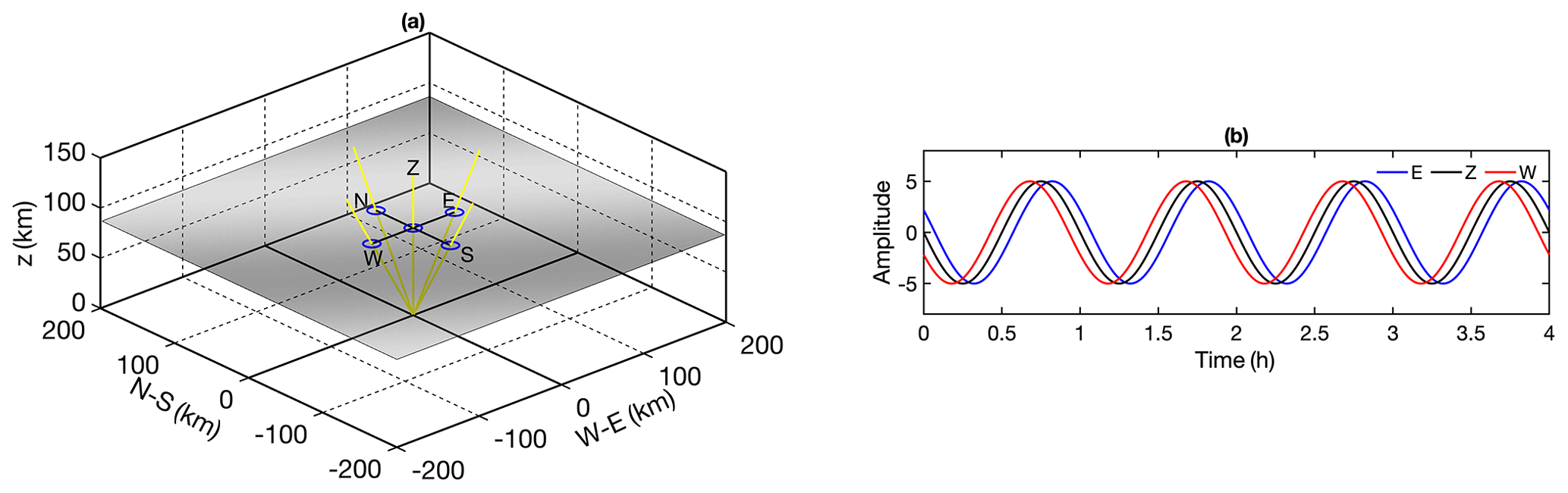
Figure 1 Panel (a) shows a lidar operated in five-direction observation mode. Yellow lines represent the laser beams pointed in five different directions, resulting from the rotation of one laser beam. The laser beam's off-zenith angle is 30°. A simulated plane wave is shown in grayscale at 90 km altitude with 400 km horizontal wavelength and the wavefront is oriented at 60° clockwise from north. Panel (b) shows the time series of simulated perturbations corresponding to the plane wave shown in (a) and retrieved from the location of E, Z, and W beams at 90 km. The wave amplitude has an arbitrary unit and the period is 1 h.

The relationship between LOS winds (V_E, V_W, V_N, V_S, V_Z) and zonal, meridional, and vertical winds (u_x, v_y, w_z) in different directions (x = E, W, y = N, S, z = E, W, N, S, Z) is described by Gardner and Liu (2007, Eq. A1) as

$$\begin{array}{}\text{(2)}& \begin{array}{rl}{\displaystyle }& {\displaystyle }{V}_{\mathrm{E}}=u_{\mathrm{E}}\sin \mathit{\alpha }+w_{\mathrm{E}}\cos \mathit{\alpha }\\ {\displaystyle }& {\displaystyle }{V}_{\mathrm{W}}=-u_{\mathrm{W}}\sin \mathit{\alpha }+w_{\mathrm{W}}\cos \mathit{\alpha }\\ {\displaystyle }& {\displaystyle }{V}_{\mathrm{N}}=v_{\mathrm{N}}\sin \mathit{\alpha }+w_{\mathrm{N}}\cos \mathit{\alpha }\\ {\displaystyle }& {\displaystyle }{V}_{\mathrm{S}}=-v_{\mathrm{S}}\sin \mathit{\alpha }+w_{\mathrm{S}}\cos \mathit{\alpha }\\ {\displaystyle }& {\displaystyle }{V}_{\mathrm{Z}}=w_{\mathrm{Z}},\end{array}\end{array}$$

where α is the off-zenith angle of laser beams. When measurements from this type of lidar were analyzed, the separations of laser beams among different directions were generally ignored. Under the assumption of the atmosphere being nearly homogenous among different laser beams and vertical winds being smaller than horizontal winds, the zonal u, meridional v, and vertical w winds are derived from LOS winds as follows:

$$\begin{array}{}\text{(3)}& \begin{array}{rl}{\displaystyle }& {\displaystyle }{u}_{\mathrm{E}}=(V_{\mathrm{E}}-V_{\mathrm{Z}}\cos \mathit{\alpha })/\sin \mathit{\alpha }\\ {\displaystyle }& {\displaystyle }{u}_{\mathrm{W}}=-(V_{\mathrm{W}}-V_{\mathrm{Z}}\cos \mathit{\alpha })/\sin \mathit{\alpha }\\ {\displaystyle }& {\displaystyle }{v}_{\mathrm{N}}=(V_{\mathrm{N}}-V_{\mathrm{Z}}\cos \mathit{\alpha })/\sin \mathit{\alpha }\\ {\displaystyle }& {\displaystyle }{v}_{\mathrm{S}}=-(V_{\mathrm{S}}-V_{\mathrm{Z}}\cos \mathit{\alpha })/\sin \mathit{\alpha }\\ {\displaystyle }& {\displaystyle }{w}_{\mathrm{Z}}=V_{\mathrm{Z}}.\end{array}\end{array}$$

Note that the derived zonal wind (u_E and u_W), meridional wind (v_N and v_S), and vertical wind (w_Z) are available in different directions and time steps, while the scalar temperature measurements are available in all five directions. The derived zonal, meridional, and vertical winds have relatively large errors. The latter wave analyses are mainly based on temperature measurements, while the winds are only shown for reference.

If a wave defined by Eq. (1) propagates through the five laser beams from a certain direction, the laser beams probe different phases of the wave, as is illustrated by Fig. 1a. There should be some phase shifts in the wave-induced perturbations of different laser beams, as shown by the simulations in Fig. 1b. In theory, phase shifts can be determined from these perturbations and further used to derive horizontal wave information. The key lies in the accurate determination of the phase shift. In this study, we utilize the cross-spectrum to retrieve the phase shifts in the wave-induced perturbations from different directions. Two time series of the same frequency ω but different phases ϕ are described by

$$\begin{array}{}\text{(4)}& \begin{array}{rl}{\displaystyle }& {\displaystyle }{y}_{\mathrm{1}}\left(t\right)=A_{\mathrm{1}}\cdot \sin \left(\mathit{\omega }t+{\mathit{\varphi }}_{\mathrm{1}}\right)\\ {\displaystyle }& {\displaystyle }{y}_{\mathrm{2}}\left(t\right)=A_{\mathrm{2}}\cdot \sin \left(\mathit{\omega }t+{\mathit{\varphi }}_{\mathrm{2}}\right).\end{array}\end{array}$$

The corresponding frequency spectra are Y₁(ω)=FFT[y₁(t)] and Y₂(ω)=FFT[y₂(t)], and the cross-spectrum between the two time series is $I_{\mathrm{12}}\left(\mathit{\omega }\right)=Y_{\mathrm{1}}\left(\mathit{\omega }\right)\cdot Y_{\mathrm{2}}^{\star }\left(\mathit{\omega }\right)$. The argument of the complex cross-spectrum is the phase difference between two waves ($\mathrm{Arg}\left[I_{\mathrm{12}}\right(\mathit{\omega }\left)\right]={\mathit{\varphi }}_{\mathrm{1}}-{\mathit{\varphi }}_{\mathrm{2}}$). Here, we treat the target waves as quasi-monochromatic, which might not reflect the realistic dispersive waves existing in the form of wave packets but preserve the main characteristics. In the wave parameter estimations, there might exist ambiguity in the phase differences. Therefore, the wave horizontal wavelength must be larger than the laser beam separation that yields a small phase difference for this method to be effective. Furthermore, the validity of the derived wave speed could be used to eliminate some unphysical results. There is also ambiguity in distinguishing the wave propagation direction. In this study, measurements from the third available direction were utilized to resolve the ambiguity. Considering the uncertainties in the measurements, the phase differences could not be too small to be distinguished. Therefore, the method is immune to the aliased signals of tides as they have much larger scales and yield tiny phase shifts within 100 km. A sensitivity study was carried out to verify the effectiveness of the method in resolving waves of different scales and periods.

This type of sodium lidar usually operates at night, with a typical duration of no longer than 10 h. The resulting resolution ($\mathrm{1}/\mathrm{10}$ h⁻¹) in the spectral domain is relatively coarse. There exist possibilities of spectral leakage and the true peaks falling between two adjacent integral spectral points. We improved the identification of the spectral peaks by applying a non-linear fitting of a parabolic function on the magnitudes of three integer spectral points close to the apparent peak. With the refined method, we hope to acquire the non-integer spectral peaks closer to the actual values and estimate the wave amplitudes A, periods τ (T is reserved to abbreviate “temperature”), and phase shifts ϕ more accurately. Given the off-zenith angle α, the spatial separation between zenith and any off-zenith directions can be calculated as $\mathrm{\Delta }=h\cdot \tan \left(\mathit{\alpha }\right)$ at altitude h. Once the phase differences in the zonal and meridional directions (ϕ_x and ϕ_y) are determined by the cross-spectral methods, the horizontal wavenumbers in the zonal and meridional directions are derived from

$$\begin{array}{}\text{(5)}& \begin{array}{rl}{\displaystyle }& {\displaystyle }k={\displaystyle \frac{\mathrm{2}\mathit{\pi }}{\mathrm{\Delta }\cdot {\mathit{\varphi }}_x}}\\ {\displaystyle }& {\displaystyle }l={\displaystyle \frac{\mathrm{2}\mathit{\pi }}{\mathrm{\Delta }\cdot {\mathit{\varphi }}_y}}.\end{array}\end{array}$$

Then, the full set of horizontal wave parameters of wavelength λ_H, propagation azimuth angle θ, and observed (ground-based) phase speed c_H can be calculated as

$$\begin{array}{}\text{(6)}& \begin{array}{rl}{\displaystyle }& {\displaystyle }{\mathit{\lambda }}_H={\displaystyle \frac{\left|k\cdot l\right|}{\sqrt{k^{\mathrm{2}}+l^{\mathrm{2}}}}}\\ {\displaystyle }& {\displaystyle }\mathit{\theta }=\arctan \left({\displaystyle \frac{l}{k}}\right)\\ {\displaystyle }& {\displaystyle }{c}_H={\displaystyle \frac{{\mathit{\lambda }}_H}{\mathit{\tau }}}.\end{array}\end{array}$$

3 Observational results

3.1 Temperature/wind perturbations and background states

On the night of 14 January 2002, the lidar was operated in five-direction mode from around 06:30 to 11:00 UT. Sodium density, temperature, and winds were continuously observed within the period as the laser was rotated in all five directions. A second-order polynomial fitting was used to remove the mean state and tidal signals. The detrended temperature measurements in different directions are shown in Fig. 2. Abundant perturbations of various periods are identified from measurements in all directions, and distinct downward phase progression is seen in the perturbations, which implies an upward wave propagation. There might exist some tide residues in the perturbations that could change the wave amplitudes, but they will not influence the estimate of the phase shift. The amplitudes of temperature perturbations reach ±10 K and there is a layered structure in the vertical direction. The wave patterns of the perturbations in different directions are similar, so they are likely the same wave packets spreading over a larger area and being captured by the laser beams in different directions. Close inspection of the temperature perturbation peaks in different directions revealed some shifts in time, resulting from the spatial separation of laser beams in different directions. The detrended perturbations of different wind components are shown in Fig. 3, in which similar wave patterns with a downward phase progression can be identified in the zonal and meridional winds, with an amplitude of up to ±20 m s⁻¹. The wave pattern is still clear in the vertical wind perturbation, with an amplitude ±2 m s⁻¹. However, the downward phase progression is less evident due to the uncertainty of vertical winds. For both temperature and winds, the measurements at the top and bottom sides are associated with larger uncertainties and should be interpreted with caution.

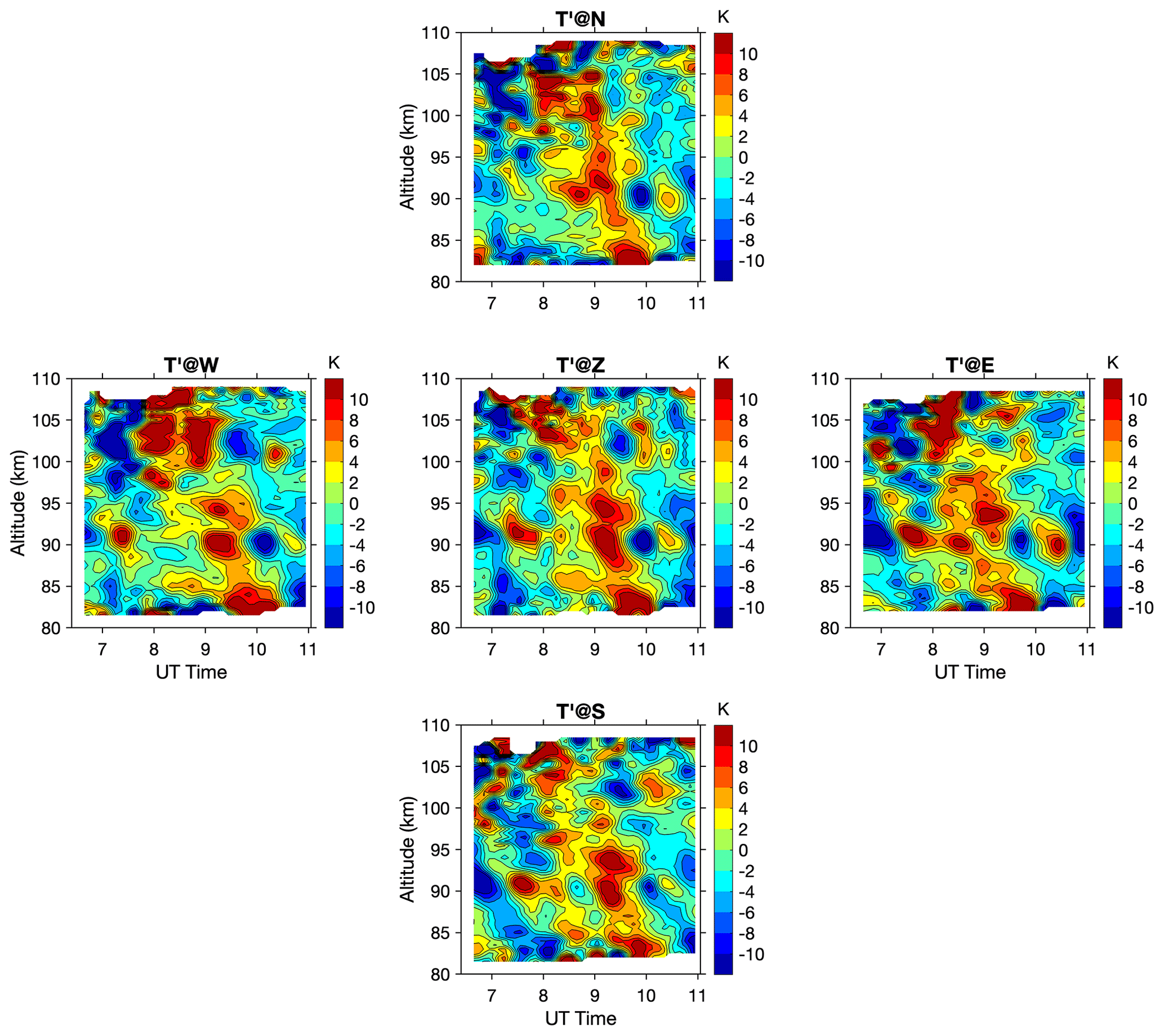
Figure 2 Detrended temperature perturbation in five different directions. The y axis of non-zenith directions is the true altitude corrected from the slant distance along the laser beam.

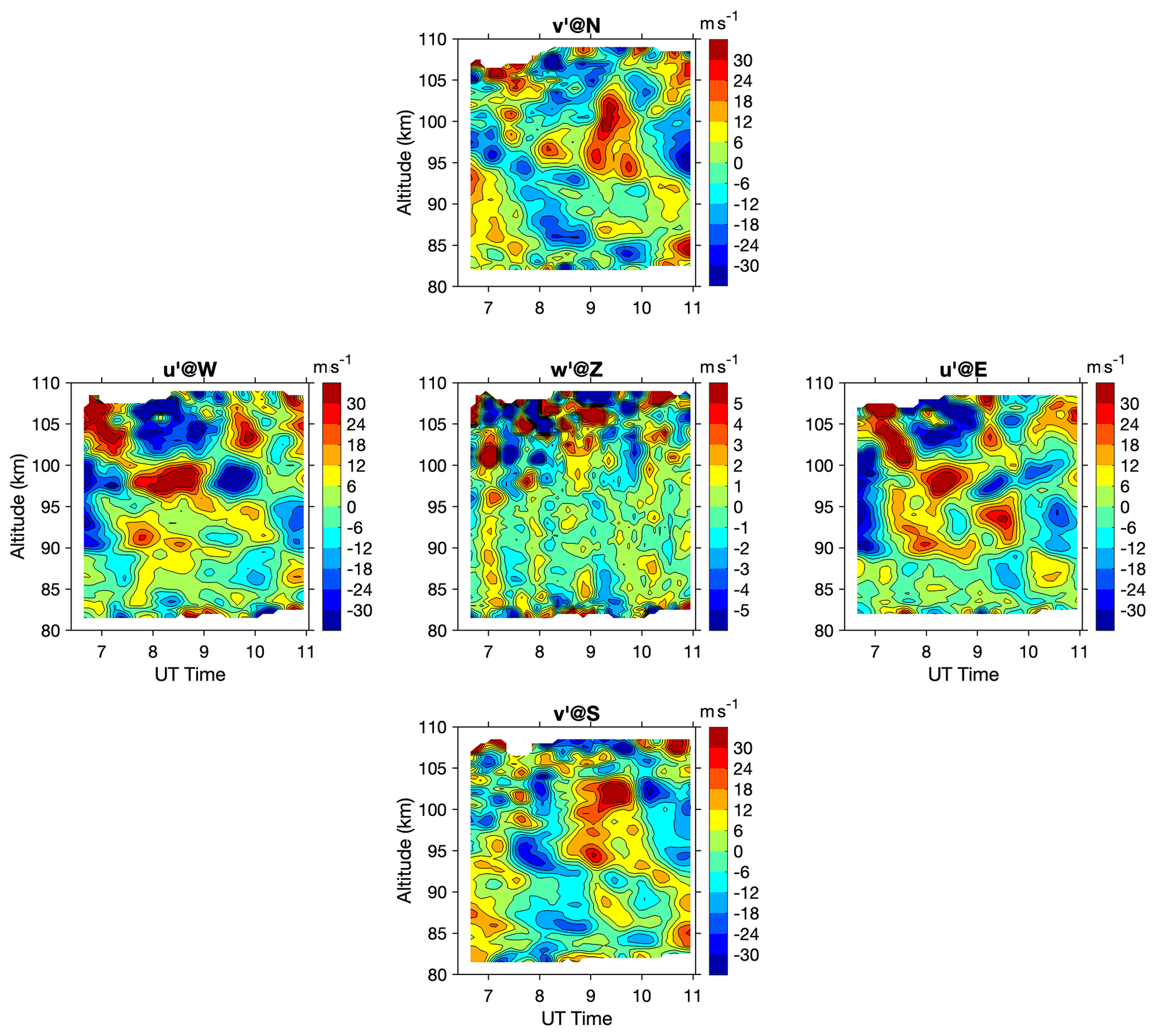
Figure 3 Detrended wind measurements in five different directions. Note that it is the zonal wind at W and E, meridional wind at S and N, and vertical wind at Z. The color scales for horizontal (zonal/meridional) and vertical winds are different.

To identify the dominant wave modes from the temperature and wind measurements, the frequency spectra were calculated from detrended temperature and wind perturbations at all altitudes. Figure 4 shows the spectra of temperature perturbation in five directions, which all show a similar pattern. The average spectrum of all five directions is shown in the upper right corner. The identified spectral peaks at each altitude using the fitting method were also denoted on the average spectrum. There might be one to several peaks at each altitude. Overall, there exist two prominent peaks; one has a period of about 3.2 h and the other one about 1.6 h. The 3.2 h period component is persistent along with the whole altitude range, and the 1.6 h peak exists mostly below 90 km and reaches a maximum at 90 km. The spectra of wind perturbation are shown in Fig. A2. The spectral peak around 3.2 h is also dominant in the horizontal (zonal and meridional) winds. However, the 1.6 h one is less evident. This is likely due to the spectral leakage of the 3.2 h wave component with much larger magnitudes which overwhelms the 1.6 h period one. The two dominant wave components need to be separated from the mean background states, variations with longer periods, and from each other for further cross-spectral analysis. Cut-off periods/frequencies are determined for desired digital filters based on the mean spectra of temperature and wind perturbations. Two spectral peaks are quite close in the frequency domain, so we used Chebyshev type II filters with flat passband and steep transition to stopband. To filter out the 1.6 h wave component, the cut-off period of a high-pass filter is selected as 2.2 h (0.46 h⁻¹).

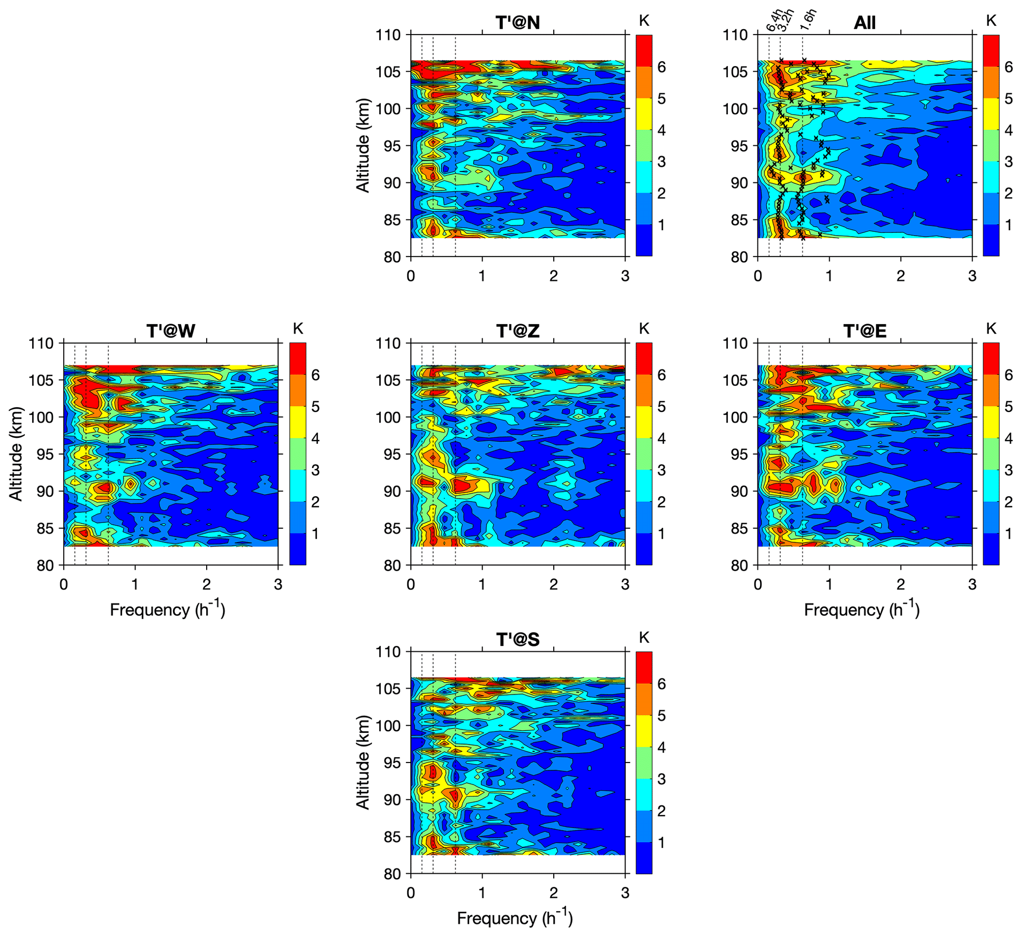
Figure 4 Spectra of detrended temperature perturbation in all five directions, and the average of all five directions is shown in the upper right corner, with black crosses marking the peaks at each altitude. (See text about the method of determining those peaks.) The vertical dashed lines denote the periods of 6.4, 3.2, and 1.6 h.

To fully understand the propagation condition of waves, the background atmosphere states were analyzed. Figure 5a–c show the background temperature T₀, zonal wind u₀, and meridional wind v₀ retrieved by detrending as defined above. The background atmosphere states show clear modulation of tides, indicated by a slow downward phase progression in both temperature and winds. The horizontal winds are quite strong, with a magnitude of ∼ 100 m s⁻¹ toward the northeast above 95 km and a magnitude of ∼ 50 m s⁻¹ toward the southeast around 85 km, and there is a relatively calm layer around 90 km. Squared buoyancy frequency N² is calculated from background temperature T₀ through

$$\begin{array}{}\text{(7)}& N^{\mathrm{2}}={\displaystyle \frac{g}{T_{\mathrm{0}}}}\left({\displaystyle \frac{\partial T_{\mathrm{0}}}{\partial z}}+{\displaystyle \frac{g}{c_p}}\right),\end{array}$$

where g is the gravity acceleration constant and c_p is the specific heat at constant pressure. Larger values of N² indicate a more statically stable atmosphere, while values of negative N² imply an unstable atmosphere. The squared buoyancy frequencies N² shown in Fig. 5d reveal that the background atmosphere was layered with a convectively stable layer between 90 and 97 km, with larger N² values about 6–8 × 10⁻⁴ s⁻². This stable layer gradually moved downward as modulated by tides. Multiple relatively unstable layers existed in between the stable layers around 87, 98, and 106 km. These layers with positive but smaller N² can also be unfavorable for wave propagation, as the resulting buoyancy period might be longer than the wave intrinsic period.

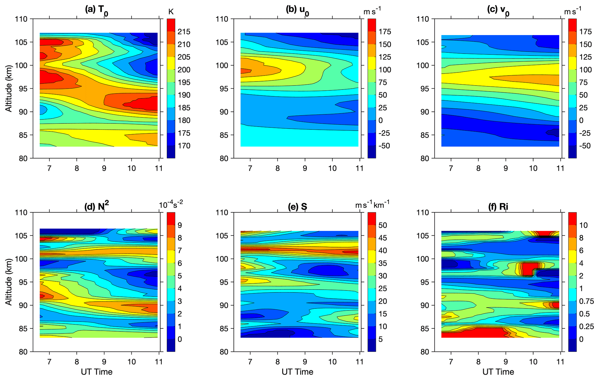
Figure 5 Background (a) temperature T₀, (b) zonal wind u₀, and (c) meridional wind v₀. Calculated (d) squared buoyancy frequency N², (e) vertical shear of horizontal wind S, and (f) Richardson number Ri.

The Richardson number Ri is commonly used to characterize the dynamical (shear) instability and is calculated through

$$\begin{array}{}\text{(8)}& \mathit{Ri}={\displaystyle \frac{N^{\mathrm{2}}}{S^{\mathrm{2}}}}={\displaystyle \frac{N^{\mathrm{2}}}{{\left(\partial u_{\mathrm{0}}/\partial z\right)}^{\mathrm{2}}+{\left(\partial v_{\mathrm{0}}/\partial z\right)}^{\mathrm{2}}}},\end{array}$$

where S is the vertical shear of the horizontal wind. The atmosphere is considered to be dynamically unstable when $\mathrm{0}<\mathit{Ri}<\mathrm{1}/\mathrm{4}$. A strong horizontal wind shear and a negative vertical temperature gradient make the atmosphere dynamically unstable. As shown in Fig. 5f, the atmosphere is in an overall stable status, with Ri approaching $\mathrm{1}/\mathrm{4}$ in a few thin layers near 87, 95, and 102 km where dynamical instability was likely to occur. Large wind shears are the main factors in these unstable areas. The layer near 90 km was relatively stable with a large N² and a small wind shear, resulting in larger Ri. This layer is favorable for the propagation of the atmospheric wave or allows wave amplitudes to reach larger values. As shown by the spectral analysis, there are two isolated wave components presented at the same time. The tides dominate the background states shown in Fig. 5. However, the longer-period (3.2 h) wave effectively acts as the background for the shorter-period (1.6 h) wave. The perturbation resulting from the longer-period wave might change the temperature gradient, and wind shear leads to a different stability condition for the shorter-period wave. The background states that include the longer-period (3.2 h) wave component are given in Fig. A6. Noticeable differences could be identified in the Ri where the relatively unstable area largely expands, especially above 95 km, which might lead to the dissipation of the shorter-period wave toward higher altitudes. However, the stable layer around 90 km also expands to a slightly wider altitude range, which improves the propagation condition for the shorter-period wave. The corresponding background states are used to diagnose each wave component in later sections.

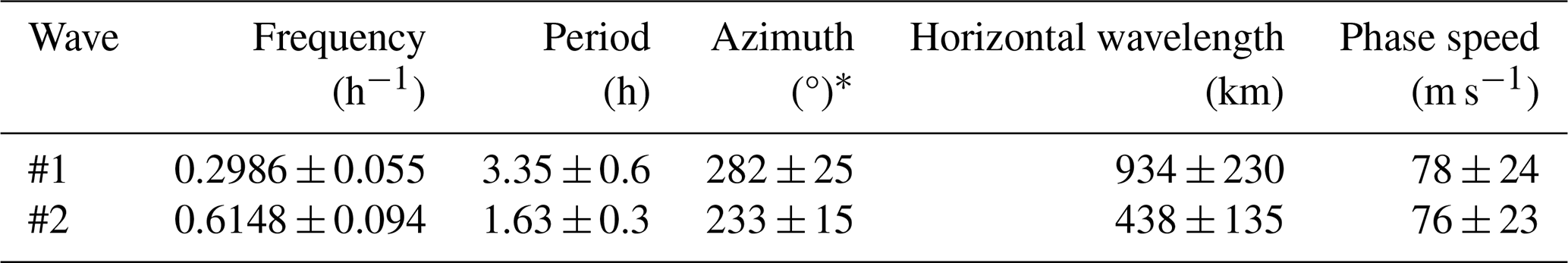
3.2 Filtered wave components and wave parameters

After applying the desired filters to the temperature and wind perturbations, the two dominant wave components are isolated. Using the improved spectral peak determination method, the best-estimated periods of the two dominant components are determined to be 3.35 h (0.2986 h⁻¹) and 1.63 h (0.6148 h⁻¹). These two wave packets are referred to as wave #1 and wave #2 in the subsequent analysis. Figure 6 shows the filtered temperature perturbations of wave #1 in all five directions, with Ri overlapped by contour lines for some values (0.25 and 0.5). The atmosphere is generally in a stable condition favorable for upward wave propagation, with only a few thin layers with Ri less than 0.25, and the layers only persist for a short time. However, the wave perturbations have larger amplitudes (about ±5 K) around these layers with a larger Richard number, making the waves appear like nodal structures. Figure 7 shows the filtered perturbations for wave #2 with one local minimum at 90 km highlighted (white crosses). The slight shift in time is visible by comparing perturbations of different directions, and the wave packet roughly moves from the northeast toward the southwest. The wave pattern and downward phase progression are visible in all directions. The perturbations reach a maximum of ±10 K at about 90 km altitude, confined within both layers above and below with smaller magnitudes of Ri. Another maximum can be seen at below 85 km. Even though there are wave patterns at higher altitudes above 100 km, the wave pattern is less consistent in different directions and shows up with varying periods. Multiple thin unstable layers exist in this altitude range, so upward propagation waves might undergo non-linear wave-mean flow interaction, resulting in wave dissipation.

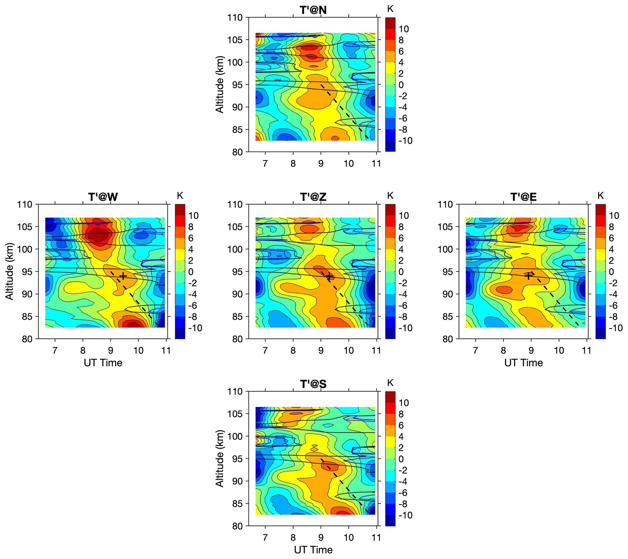
Figure 6 Filtered temperature perturbation for wave #1 (3.35 h period) in five different directions. Overlapped contours are the Ri with values 0.25 in blue and 0.5 in black. The dashed black lines mark the potential downward phase progression and are fixed among different panels. The black crosses indicate one local maximum at 94 km, helping to distinguish the phase shift in time. The wavefront moves from E to W.

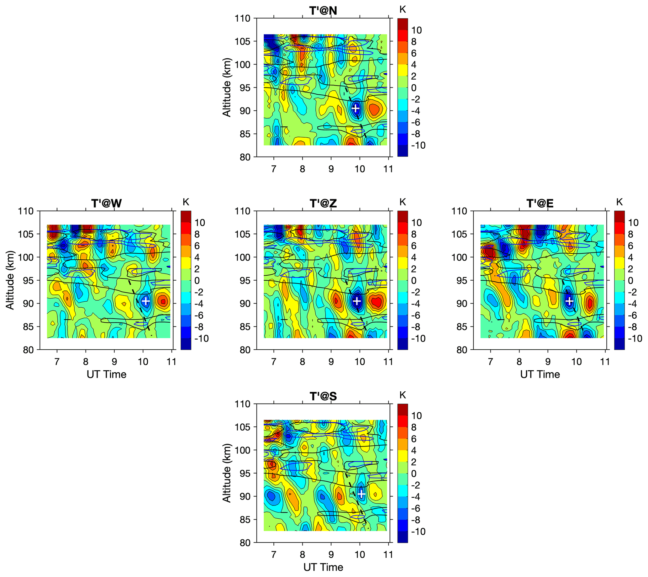
Figure 7 Filtered temperature perturbation for wave #2 (1.63 h period) in five different directions. Overlapped contours are the Ri with values 0.25 in blue and 0.5 in black. The dashed black lines mark the potential downward phase progression and are fixed among different panels. The white crosses indicate one local minimum at 90 km, helping to distinguish the phase shift in time. The wavefront moves from E to W and N to S.

Filtered wind perturbations are shown in Figs. A4 and A5. The signatures of both waves are evident in the horizontal winds but with less evident downward phase progression. The node structure is clear in the vertical direction with at least two maxima at different altitudes. The wave patterns are slightly different in the zonal, meridional, and vertical winds, as the relations are determined by the polarization formulas. Even though the wave pattern is clear, the phase shifts among measurements of different directions are imperceptible in horizontal wind perturbations for both wave packets. The measurement uncertainties of 5–10 m s⁻¹ are too large compared with the wave amplitudes of 10–20 m s⁻¹, making the slight phase shift hard to distinguish. In later analysis, only the temperature measurements are used for the cross-spectral method to estimate wave parameters.

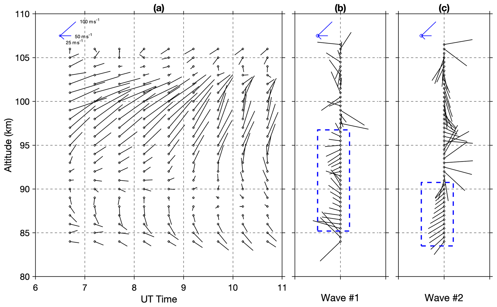
Figure 8 Panel (a) shows the background winds, (b) the horizontal phase speed of wave #1, and (c) the horizontal phase speed of wave #2. The staff points to the directions to which the wind blows, or the wave propagates toward, and the length represents the wind speed or phase speed magnitudes. The unit ratio of the axis scale (5 km = 1 h) matches the zonal and meridional components of the wind and wave speeds to let the staff point in the right direction on the plane. The boxes in (b) and (c) mark the altitude range where the mean and uncertainties are estimated. The legends in the upper left corner of each panel denote the speeds of 100, 50, and 25 m s⁻¹ at the NE, E, and SE directions, respectively.

Table 1 Gravity wave parameters retrieved from lidar measurements in the ground-based observing frame.

^∗ The azimuth angle is measured clockwise from the north.

Using the proposed method detailed in Sect. 2, we choose the temperature measurements at four off-zenith directions to derive the phase shifts in the zonal and meridional directions, and horizontal wavelength, propagation azimuth, and observed phase speed were then calculated. In Fig. 8, the background wind and wave phase speed at different altitudes are shown in the “wind barb” manner, with the length representing speed and the staff pointing to the direction to which the wind blows and toward which the wave propagates. In Fig. 8b and c, wind barb does not exist at some altitudes because the derived wave phase speed is too large ($c-u_{\mathrm{0}}>\mathrm{0.5}{c}_{\mathrm{s}}$) (Zhou and Morton, 2007), invalidating the results. Here, the speed of sound c_s in the atmosphere is estimated as $c_{\mathrm{s}}=\sqrt{\mathit{\gamma }R{T}_{\mathrm{0}}}$, where γ is the ratio of specific heat, R is the ideal gas constant, and T₀ is the background temperature. The typical speed of sound c_s is calculated to be around 280 m s⁻¹ in the lidar observation altitude range. During the lidar observation period and altitude range, the background wind is mostly toward the east, with strong northeastward winds above 95 km and moderate southeastward winds around 85 km. The calculated propagation azimuth and phase speed are relatively consistent with altitude ranges within blue boxes in Fig. 8b and c, including 85–97 km for wave #1 and below 90 km for wave #2. In addition, both wave packets are estimated to propagate opposite to the background winds, with wave #1 propagating mostly toward W and wave #2 propagating toward W–SW. In ideal conditions, these ground-observed wave parameters are invariant if the wave pattern sustains and does not dissipate. The wave parameters of frequency/period, propagation azimuth, phase speed, and horizontal wavelength, as well as their uncertainties, represented by the mean and standard derivation within the most reliable altitude range (within blue boxes in Fig. 8), are listed in Table 1. Both frequency/period and phase speed are estimated in a ground-based frame. The horizontal wavelengths of wave #1 and wave #2 are estimated to be around 934 and 438 km, both with a ∼ 20 % uncertainty. The propagation azimuth angles are estimated to be 282 and 233° for the two waves, both with a 15–25° uncertainty. These wavelengths and azimuths correspond to phase shifts of −36 and 8° between measurements of E–W and N–S for wave #1, and phase shifts of −65 and −49° for wave #2. The 8° phase shift in the N–S direction for wave #1 is too small and hardly visible in Fig. 6. The observed phase speeds of the two wave packets are quite similar, around 80 m s⁻¹. Both waves propagate through the background atmosphere with varying stability and potentially undergo some dissipation and dispersion, especially at higher altitudes. Therefore, the monochromatic wave assumption is no longer satisfied there, and wave speed and azimuth determined from the phase shift show large fluctuations at these altitudes. The wave pattern shows downward phase progression in the vertical direction, and not a single complete wave cycle is identified within the altitude range. Therefore, the vertical wavelengths were roughly estimated from the phase slope to be larger than 10 km for both wave packets.

3.3 Wave diagnosis: dispersion and polarization relations

In linearized gravity wave theory, the dispersion relation links the vertical wavenumber to the horizontal wave parameters and background states. It is often used to diagnose gravity wave propagation, reflection, and ducting. For the acoustic–gravity waves in a compressible atmosphere, Eqs. (9) and (10) in Zhou and Morton (2007) are full descriptions of the dispersion relation. For waves with a small intrinsic horizontal phase speed ($|c-\stackrel{\mathrm{‾}}{u}|<\mathrm{0.5}{c}_{\mathrm{s}}$), which is valid for most observed gravity waves, the dispersion relation can be described as

$$\begin{array}{}\text{(9)}& \begin{array}{rl}{m}^{\mathrm{2}}& ={\displaystyle \frac{N^{\mathrm{2}}}{(c-\stackrel{\mathrm{‾}}{u}{)}^{\mathrm{2}}}}-k_H^{\mathrm{2}}-{\displaystyle \frac{\mathrm{1}}{\mathrm{4}{H}_{\mathrm{s}}^{\mathrm{2}}}}+{\displaystyle \frac{\mathrm{1}}{c-\stackrel{\mathrm{‾}}{u}}}{\displaystyle \frac{{\mathrm{d}}^{\mathrm{2}}\stackrel{\mathrm{‾}}{u}}{\mathrm{d}{z}^{\mathrm{2}}}}\\ & +{\displaystyle \frac{\mathrm{2}-\mathit{\gamma }}{\mathit{\gamma }}}{\displaystyle \frac{\mathrm{1}}{H_{\mathrm{s}}\left(c-\stackrel{\mathrm{‾}}{u}\right)}}{\displaystyle \frac{\mathrm{d}\stackrel{\mathrm{‾}}{u}}{\mathrm{d}z}}-{\displaystyle \frac{\mathrm{3}}{c_{\mathrm{s}}^{\mathrm{2}}}}{\left({\displaystyle \frac{\mathrm{d}\stackrel{\mathrm{‾}}{u}}{\mathrm{d}z}}\right)}^{\mathrm{2}}\\ & +{\displaystyle \frac{g}{H_{\mathrm{s}}{\left(c-\stackrel{\mathrm{‾}}{u}\right)}^{\mathrm{2}}}}{\displaystyle \frac{\mathrm{d}{H}_{\mathrm{s}}}{\mathrm{d}z}}+{\displaystyle \frac{\mathrm{1}}{\mathrm{2}{H}_{\mathrm{s}}}}{\displaystyle \frac{{\mathrm{d}}^{\mathrm{2}}{H}_{\mathrm{s}}}{\mathrm{d}{z}^{\mathrm{2}}}}-{\displaystyle \frac{\mathrm{3}}{\mathrm{4}}}{\left({\displaystyle \frac{\mathrm{1}}{H_{\mathrm{s}}}}{\displaystyle \frac{\mathrm{d}{H}_{\mathrm{s}}}{\mathrm{d}z}}\right)}^{\mathrm{2}}\\ & -{\displaystyle \frac{\mathrm{1}}{H_{\mathrm{s}}\left(c-\stackrel{\mathrm{‾}}{u}\right)}}{\displaystyle \frac{\mathrm{d}\stackrel{\mathrm{‾}}{u}}{\mathrm{d}z}}{\displaystyle \frac{\mathrm{d}{H}_{\mathrm{s}}}{\mathrm{d}z}},\end{array}\end{array}$$

where $H_{\mathrm{s}}=R{T}_{\mathrm{0}}/g$ is the density scale height and γ is the ratio of specific heat, and c, $\stackrel{\mathrm{‾}}{u}$, and c_s are the observed horizontal phase speed, background wind speed in the direction of wave propagation, and speed of sound, respectively. Horizontal wavenumber k_H is related to k and l through $k_H^{\mathrm{2}}=k^{\mathrm{2}}+l^{\mathrm{2}}$. The term $c-\stackrel{\mathrm{‾}}{u}$ is the intrinsic horizontal phase speed, usually denoted as $\widehat{c}$. The corresponding intrinsic wave frequency is related to the observed wave frequency by $\widehat{\mathit{\omega }}=\mathit{\omega }-k_H\cdot \stackrel{\mathrm{‾}}{u}$. When the atmosphere is treated as incompressible where the acoustic wave is eliminated, and background temperature varies slowly within the vertical wavelength of the wave, we have c_s→∞ and $\mathrm{d}{H}_{\mathrm{s}}/\mathrm{d}z\to \mathrm{0}$.

The dispersion relation (Eq. 9) is reduced to the following form that is derived based on Taylor–Goldstein equation (Nappo, 2012, Eq. 2.34):

$$\begin{array}{}\text{(10)}& \begin{array}{rl}{m}^{\mathrm{2}}& ={\displaystyle \frac{N^{\mathrm{2}}}{{\left(c-\stackrel{\mathrm{‾}}{u}\right)}^{\mathrm{2}}}}-k_H^{\mathrm{2}}-{\displaystyle \frac{\mathrm{1}}{\mathrm{4}{H}_{\mathrm{s}}^{\mathrm{2}}}}+{\displaystyle \frac{\mathrm{1}}{\left(c-\stackrel{\mathrm{‾}}{u}\right)}}{\displaystyle \frac{{\mathrm{d}}^{\mathrm{2}}\stackrel{\mathrm{‾}}{u}}{\mathrm{d}{z}^{\mathrm{2}}}}\\ & +{\displaystyle \frac{\mathrm{2}-\mathit{\gamma }}{\mathit{\gamma }}}{\displaystyle \frac{\mathrm{1}}{H_{\mathrm{s}}\left(c-\stackrel{\mathrm{‾}}{u}\right)}}{\displaystyle \frac{\mathrm{d}\stackrel{\mathrm{‾}}{u}}{\mathrm{d}z}}.\end{array}\end{array}$$

The coefficient of the last term in Eq. (10) is different from the original one due to a correction for a compressible atmosphere based on discussions in Zhou and Morton (2007). If the wind shear terms are further neglected, the dispersion relation (Eq. 10) is simplified to Eq. (24) in Fritts and Alexander (2003) but without the Coriolis term and is also the same as the dispersion relation derived by Hines (1960):

$$\begin{array}{}\text{(11)}& m^{\mathrm{2}}={\displaystyle \frac{N^{\mathrm{2}}}{{\left(c-\stackrel{\mathrm{‾}}{u}\right)}^{\mathrm{2}}}}-k_H^{\mathrm{2}}-{\displaystyle \frac{\mathrm{1}}{\mathrm{4}{H}_{\mathrm{s}}^{\mathrm{2}}}}.\end{array}$$

Through the dispersion equations, the vertical wavenumber m is related to the wave characteristics, including the horizontal wavenumbers k_H and phase speed c, and the background states, including the projected wind on wave propagation direction $\stackrel{\mathrm{‾}}{u}$ and wind shear, as well as the background temperature T₀ and its gradient as reflected by scale height H_s and buoyancy frequency N. In the regions of the atmosphere where m²>0, gravity waves are able to propagate freely and are characterized by corresponding m, k, l, and c. Regions of m²<0 indicate evanescence for gravity waves, where wave amplitudes decay exponentially. When a propagating wave encounters a region where m²<0, partial or total reflection can occur depending on the depth of the evanescent region. Gravity waves whose propagation is restricted in a region with reflective regions of evanescence, above and below, are said to be ducted. At altitudes where $c=\stackrel{\mathrm{‾}}{u}$, the vertical wavenumber approaches infinity, and the waveform is overturned, so wave breaking or dissipation occurs. The phenomenon is called wave critical-layer filtering, which could be partial or total. In this case study, the altitude range is limited to within 85–105 km, during which the background temperature gradient is about −5 K km⁻¹ and the wind shear is as strong as 30 m s⁻¹ km⁻¹. The contribution of terms related to the temperature gradient and wind shear is not insignificant. Since all wave parameters and background states are explicitly determined, we evaluated all three forms of dispersion relations to diagnose the propagation of the identified wave packets.

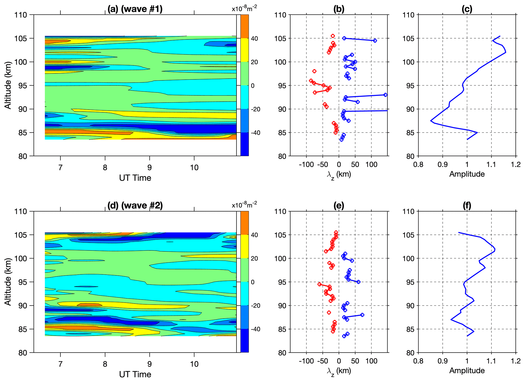
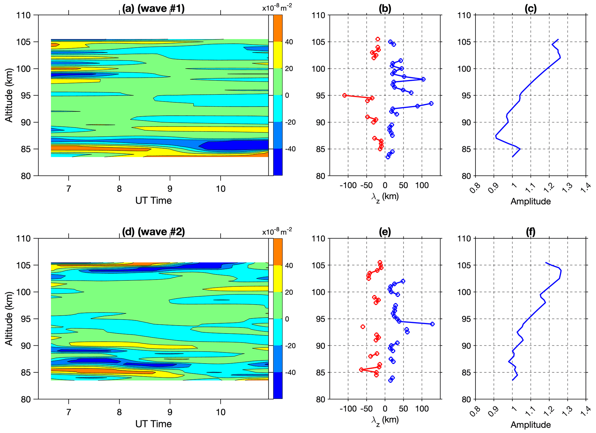
Figure 9 Calculated m² for (a) wave #1 (3.35 h) and (d) wave #2 (1.63 h) using Eq. (9), as well as the vertical wavelength derived from the mean m² for (b) wave #1 and (e) wave #2. The negative wavelengths correspond to the evanescent regions. The relative wave amplitude is estimated from the combined decay and growth for (c) wave #1 and (f) wave #2.

Figure 9a and d show the calculated m² for the two retrieved wave packets based on the full dispersion relation of Eq. (9). The m² shows up in layered structures for both waves, potentially creating ducts for the gravity waves. For the 3.35 h wave (#1), there are major layers of negative m² around 85–86, 95, 98, and 103 km altitudes. There are also several thin layers of negative m² at other altitudes lasting shorter times. When upward propagating waves encounter the layers, their amplitudes will attenuate on top of the growth due to decreased atmospheric density. For the evanescent layer around 85–86 km, the waves are supposed to dampen at a fast rate (larger value of i×m). However, as this layer is thin, with a maximum thickness of 2 km, plenty of wave energy could penetrate the layer to higher altitudes. This also applies to other thin evanescent layers where the attenuation is even less. The upward propagating waves were partially reflected and refracted at each evanescent layer, which could change the wavefront orientation. The partial refraction/reflection was also presented by the previous numerical simulations in similar scenarios (Heale et al., 2014; Cao et al., 2016). For the temperature perturbation in Fig. 6, the wave pattern shows up with a nodal structure with clear amplitude maximums around 85, 92, and 102 km, and discontinuities in the phase progression in the vertical direction. These features directly result from the partial reflection and refraction at the multiple evanescent layers where the perturbations observed by the lidar are the superposition of incident and reflected waves between the evanescent layers. For the 1.63 h wave (#2), the overall layered structure in m² remains similar to the 3.35 h wave. However, the 3.35 h wave effectively changes wind and temperature, as well as creates differences in m², and leads to different propagation conditions for the 1.63 h wave. The evanescent layer around 86 km reduced the attenuation rate from 09:00 UT onwards, which largely increased the portion of the transmission of wave energy. In addition, the 3.35 h wave increased the evanescent layer thickness to 5 km around 95 km, which could limit the transmissible wave energy to further altitudes. As shown in Fig. 7, there is a visible maximum below 85 km, and another maximum was around 90 km, whose wave amplitudes largely increased after 09:00 UT. The amplitudes decreased dramatically right above 95 km; however, some wave peaks can be seen above 100 km. The average m² profiles of the whole period are calculated for both wave packets and the corresponding vertical wavelengths are estimated and shown in Fig. 9b and d. The positive vertical wavelengths for the freely propagating waves are about 15–20 km for wave #1 and 10–15 km for wave #2, similar to the ones estimated from the downward phase progression slope. The negative wavelength corresponds to the evanescent region and is equivalent to the scale height of the wave amplitude decay. The overall decay/growth rate of the wave amplitude is described by $e^{(\mathrm{1}/\mathrm{5}{H}_{\mathrm{s}}-im)z}$, where decay occurs when m is an imaginary number in the evanescent region. The factor of 5H_s, rather than 2H_s, was chosen to mimic wave dissipation; otherwise, the wave amplitude would grow too fast. In Fig. 9c and f, the relative wave amplitudes are estimated, assuming one unit of wave amplitude at the lowest altitude. The predicted wave amplitude shows fluctuation and several maxima at different altitudes, which are the combined efforts of evanescent decay and conserved growth. The evanescent layers at different altitudes would attenuate the wave amplitude, but layers with the time-varying m² could reduce the dampening efforts and spare more energy penetrating to higher altitudes. Bossert et al. (2014) presents case studies using lidar observations and simulations to show high-frequency (period shorter than 15 min) gravity waves propagating to higher altitudes through alternating regions of evanescence and free propagation over a few kilometers. In this study, the two medium-frequency wave packets observed by the lidar propagate through multiple thin and time-varying evanescent layers with a good portion of wave energy penetrating to higher altitudes, and partial reflection and refraction occur with the observed amplitude maxima found between these evanescent layers.

The m² estimated by Eqs. (10) and (11) are shown in Figs. A7 and A8. The results of Eq. (10) show overall similarity with the ones of Eq. (9), but some differences exist. The evanescent layers estimated by Eq. (10) are slightly thinner, which shows the contribution of neglected temperature gradients. The m² calculated by Eq. (11) fails to capture most of the layered structures and underestimates all evanescent layer thickness as wind shear is a significant contributing factor for both waves. As discussed above, inconsistency exists among different dispersion relations, and some simplifications fail to capture the authentic characters. In the application of dispersion relations, the full background temperature and wind measurements might not be available in all cases or are sometimes limited only to a few altitudes. Nevertheless, simplified formulas (Eqs. 10 and 11) can be best utilized to diagnose wave propagation; however, the results should be interpreted with caution.

Another important relation derived from linearized wave equations is the polarization relation that describes the relative phase differences and amplitude ratios of various wave quantities. If gravity waves do not undergo dissipation, the complex wave amplitudes of the relative temperature $\stackrel{\mathrm{̃}}{T}\left(T^{\prime }/\stackrel{\mathrm{‾}}{T}\right)$, zonal wind $\stackrel{\mathrm{̃}}{u}$, meridional wind $\stackrel{\mathrm{̃}}{v}$, and vertical wind $\stackrel{\mathrm{̃}}{w}$ should satisfy the following polarization relations (Fritts and Alexander, 2003; Vadas, 2013; Lu et al., 2015):

$$\begin{array}{}\text{(12)}& \begin{array}{rl}{\displaystyle \frac{\stackrel{\mathrm{̃}}{T}}{\stackrel{\mathrm{̃}}{w}}}=& {\displaystyle \frac{N^{\mathrm{2}}\left(im+\frac{\mathrm{1}}{\mathrm{2}{H}_{\mathrm{s}}}\right)-\frac{{\widehat{\mathit{\omega }}}^{\mathrm{2}}}{\mathit{\gamma }{H}_{\mathrm{s}}}\left(\mathit{\gamma }-\mathrm{1}\right)}{g\widehat{\mathit{\omega }}\left(-m-\frac{i}{\mathrm{2}{H}_{\mathrm{s}}}+\frac{i}{\mathit{\gamma }{H}_{\mathrm{s}}}\right)}}\\ {\displaystyle \frac{\stackrel{\mathrm{̃}}{T}}{\stackrel{\mathrm{̃}}{u}}}=& {\displaystyle \frac{N^{\mathrm{2}}\left(im+\frac{\mathrm{1}}{\mathrm{2}{H}_{\mathrm{s}}}\right)-\frac{{\widehat{\mathit{\omega }}}^{\mathrm{2}}}{\mathit{\gamma }{H}_{\mathrm{s}}}\left(\mathit{\gamma }-\mathrm{1}\right)}{g}}\\ {\displaystyle }& {\displaystyle \frac{\left({\widehat{\mathit{\omega }}}^{\mathrm{2}}-f^{\mathrm{2}}\right)\left(k\widehat{\mathit{\omega }}-ifl\right)}{\left(N^{\mathrm{2}}-{\widehat{\mathit{\omega }}}^{\mathrm{2}}\right)\left(k^{\mathrm{2}}{\widehat{\mathit{\omega }}}^{\mathrm{2}}+f^{\mathrm{2}}{l}^{\mathrm{2}}\right)}}\\ {\displaystyle \frac{\stackrel{\mathrm{̃}}{u}}{\stackrel{\mathrm{̃}}{v}}}=& {\displaystyle \frac{i\widehat{\mathit{\omega }}k-fl}{i\widehat{\mathit{\omega }}l+fk}}.\end{array}\end{array}$$

The complex amplitudes of $\stackrel{\mathrm{̃}}{T}/\stackrel{\mathrm{̃}}{w}$, $\stackrel{\mathrm{̃}}{T}/\stackrel{\mathrm{̃}}{u}$, and $\stackrel{\mathrm{̃}}{u}/\stackrel{\mathrm{̃}}{v}$ describe the amplitude and phase relations among different wave quantities. On the one hand, the missing quantities of observed gravity waves can be estimated through these relations assuming non-dissipation. On the other hand, the discrepancies between observed and theoretical values can be used to indicate wave dissipation. It is also possible to estimate higher-order statistical quantities, such as gravity wave momentum flux $\left(\stackrel{\mathrm{‾}}{u^{\prime }{w}^{\prime }}\right)$ and heat flux $\left(\stackrel{\mathrm{‾}}{w^{\prime }{T}^{\prime }}\right)$, from these relationships with limited observations (Liu, 2009; Guo et al., 2017).

Table 2 Amplitude (A) ratio and phase (ϕ) difference between quantities of $\stackrel{\mathrm{̃}}{T}$ and $\stackrel{\mathrm{̃}}{w}$, $\stackrel{\mathrm{̃}}{T}$ and $\stackrel{\mathrm{̃}}{u}$, as well as $\stackrel{\mathrm{̃}}{u}$ and $\stackrel{\mathrm{̃}}{v}$.

^a $\stackrel{\mathrm{̃}}{T}$ here is relative temperature perturbation $T^{\prime }/\stackrel{\mathrm{‾}}{T}$ expressed in percentage. ^b The mean and standard derivation of the quantities are calculated within the corresponding altitude range. ^c The altitude range of 85–100 km was used to calculate the mean and standard deviation.

The predicted values of $\stackrel{\mathrm{̃}}{T}/\stackrel{\mathrm{̃}}{w}$, $\stackrel{\mathrm{̃}}{T}/\stackrel{\mathrm{̃}}{u}$, and $\stackrel{\mathrm{̃}}{u}/\stackrel{\mathrm{̃}}{v}$ can be calculated from Eq. (12) with the retrieved wave and background parameters. They are complex numbers, with their absolute magnitudes representing the wave amplitude (A) ratio and phases representing the phase (φ) difference between any two quantities. Two sets of amplitude ratios and phase differences are calculated, one for positive m² and the other for negative m², corresponding to the wave free-propagating and evanescent regions. Table 2 lists the predicted results for both wave packets. In the region of free propagating, the values are relatively constant; the variations are mainly because of the change in intrinsic frequency along altitudes. However, large variations exist for the phase differences in the evanescent region. In this case, the wave packets propagate through multiple evanescent layers where partial reflection occurs. The lidar observed perturbations are the superposition of incident and reflected waves, and the propagating waves also undergo dissipation. It is difficult to accurately estimate the amplitude ratios and phase differences from the observed perturbations. Another difficulty is that the horizontal winds are not retrieved at the zenith direction and have to be indirectly estimated from horizontal winds at off-zenith directions by correcting the phase shift. Therefore, we only estimate the averaged amplitude ratios from the observations. In Table 2, the observed results are estimated with larger uncertainties, and all show discrepancies with the predicted ones. However, the observed values of $A\left(\stackrel{\mathrm{̃}}{T}\right)/A\left(\stackrel{\mathrm{̃}}{u}\right)$ are closer to the predicted ones in the evanescent region. The uncertainties in the wind measurements and wave dissipation could also contribute to this. For the ratio $A\left(\stackrel{\mathrm{̃}}{T}\right)/A\left(\stackrel{\mathrm{̃}}{w}\right)$, it is much smaller than the predicted values, which implies that the observed perturbations in the vertical wind might contain large errors. The presented results reveal the complexity of gravity waves propagating in the atmosphere. The polarization relation is good for diagnosing the free propagating waves without being reflected and refracted, and dissipation is not severe. It might not be proper when complicated wave-mean flow interaction occurs, such as in this wave case.

Using the proposed cross-spectral method, we identified two gravity wave packets and retrieved all the wave parameters, as well as determined the background states. The fully retrieved information was used to validate the linear gravity wave theories with the least assumptions. Consistent results are obtained from the diagnostic analyses using the dispersion relation, partly explaining the wave observations. However, raw lidar measurement uncertainties exert difficulties in some wave parameter estimations and diagnostic analyses using the polarization relation. In the next section, we implement a sensitivity study to evaluate the general usage of this method in detecting gravity waves.

4 Sensitivity study

It is well known that most observation techniques are restricted by the “observation filter” effect in resolving atmospheric waves. These techniques are sensitive to certain parts of the spatial and temporal spectra of the waves. The effect also applies to the lidar and the wave extraction method presented in this study. To find a spectral range of gravity waves that is more favorable to be identified by this method, we did a sensitivity study using a forward simulation. The accuracy of the cross-spectral methods in recovering the wave parameters of amplitude, period, and phase shift is quantified.

The off-zenith angle of laser beams coupled with steerable telescopes could be adjusted. However, this configuration is no longer available, and newer lidar systems are equipped with multiple fixed telescopes pointing to certain directions; thus, the off-zenith direction and angle are fixed. The photon integration time at each direction and the laser beam rotating sequence could be changed based on applications, such as only one direction in the zonal and meridional directions. There are also some lidar systems with one master laser beam being split and shooting to multiple directions simultaneously. The typical photon integration time at each direction is about 1 min to several minutes. A configuration similar to the lidar deployed in Maui is utilized in the simulation where a 30° off-zenith angle corresponds to a separation of ∼ 100 km at 90 km altitude between two off-zenith directions (W and E, or S and N). For simplicity, the temporal resolution was selected as a uniform 6 min in all directions. Because the retrieval of wave parameters in the zonal and meridional directions (k and l) is independent, the simulations only consider measurements from two laser beams aligned in one direction. The perturbations of a traveling gravity wave observed by two laser beams are described by

$$\begin{array}{}\text{(13)}& \begin{array}{rl}{\displaystyle }{y}_{\mathrm{1}}& {\displaystyle }=A\cdot \sin (\mathit{\omega }\cdot t+{\mathit{\varphi }}_{\mathrm{1}})+{\mathit{\delta }}_{\mathrm{1}}\\ {\displaystyle }{y}_{\mathrm{2}}& {\displaystyle }=A\cdot \sin (\mathit{\omega }\cdot t+{\mathit{\varphi }}_{\mathrm{2}})+{\mathit{\delta }}_{\mathrm{2}},\end{array}\end{array}$$

of which the definitions of the terms are the same as in Eq. (4). Extra terms δ₁ and δ₂, two independent (associated with different “seeds” of the pseudorandom number generator) sets of Gaussian-distributed random numbers, are introduced to mimic the uncertainties in measurements. The cross-spectral method is applied on the data (y₁, y₂) to retrieve the wave amplitude A, period $\mathit{\tau }=\mathrm{2}\mathit{\pi }/\mathit{\omega }$, and phase shift $\mathrm{\Delta }\mathit{\varphi }={\mathit{\varphi }}_{\mathrm{1}}-{\mathit{\varphi }}_{\mathrm{2}}$. To qualify the accuracy, the percentage errors of wave amplitude A, period τ, and phase difference Δϕ between the retrieved results and preset values are calculated.

In the simulation, the wave amplitude A was selected as two (with an arbitrary unit) and the random noise δ had a standard deviation of 0.5. Therefore, the following simulation and discussion only apply to this signal-to-noise ratio ($A/\mathit{\delta }$). In the simulation, 5 h of data (50 data points) were used. In order to recover the spectral peaks falling between two integer spectral points, the aforementioned fitting method was used to best retrieve the actual peaks. The horizontal wavelength was selected to vary from 300 to 3000 km (3–30 times the laser beam separation) and the period range was from 1 to 5 h. In Fig. 10, the percentage errors of wave amplitude (A), period (τ), and phase shift (Δϕ) are shown. The retrieved wave amplitudes have an error of 10 % from the true value for all periods and wavelengths. A slight negative bias of 5 % and a wave pattern are identified in amplitude errors. The retrieved periods have a 5 % error for periods shorter than 3 h and up to 10 %–20 % for waves with longer periods and shorter wavelengths. The phase shift has the largest error among these wave parameters, with errors up to 20 % for waves with wavelengths shorter than 2000 km and up to 60 % for the waves with longer horizontal wavelengths (2000–3000 km). The errors in phase shift are independent of the wave periods. The cross-spectral method is likely unable to retrieve the small phase shifts (≤ 18°) resulting from waves with larger scales, which include the residues or aliased signals from tides that often have planetary scales.

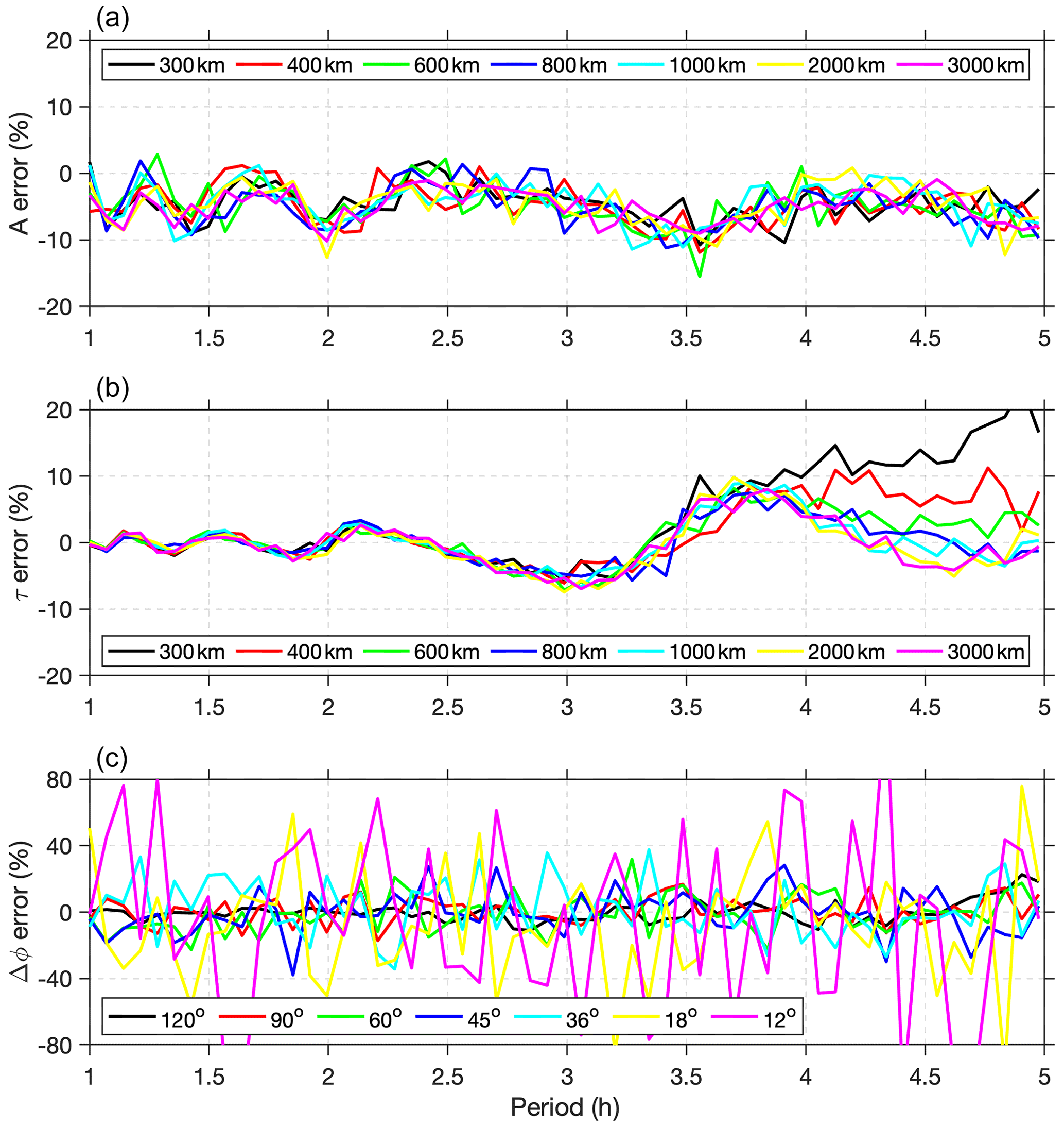
Figure 10 Percentage errors of (a) amplitude A, (b) period τ, (c) phase shift Δϕ, between the retrieved results and preset values, for gravity wave packets with different periods (1–5 h) and wavelengths (300–3000 km). The phase shifts Δϕ of 120–12° result from a 100 km separation between two laser beams, corresponding to a 300–3000 km wavelengths.

The proposed method relies on cross-spectral analysis and inherits the typical drawback of any spectral method. In this simulation, there is only one frequency being simulated. If spectral leakage is not an issue when the actual peak is close to the integer spectral points, the wave parameters could be determined accurately. However, with limited samples, the resolution in the spectral domain is coarse, and there is a chance of spectral leakage that the actual peaks fall between two integer spectral points. The negative bias of the retrieved amplitude and the wave pattern in the errors of the wave parameters (A and τ) are related to spectral leaks. When multiple wave components are mixed together, the spectral leakage will be more complicated and limit wave identification. With measurements from only two directions, the retrieved wavelength and phase speed are apparent ones along that direction. The actual wavelength and speed in any direction can be the composition of apparent ones in the zonal and meridional directions. As narrow-band resonance lidars usually provide measurements over an altitude range between 80 and 110 km, the wave propagating in the vertical direction can be captured. The retrieved period, wavelength, and phase speed are invariant if the waves do not undergo severe dissipation. This could provide another level of verification of the retrieved wave parameters at different altitudes.

Here, we provide an introductory assessment of the proposed wave extraction method. The data duration is critical, as more data points could help alleviate the spectral leakage and retrieve accurate wave parameters. However, the duration is limited by the operation of such type of lidar that mostly works at night unless extra filters are used to facilitate daytime operation (Chen et al., 1996). There is a trade-off between longer datasets for higher spectral resolution and the duration of wave presence with an invariant period and amplitude. The most favorable wave period of this method is limited to be shorter than the data duration, to minimize the spectral leakage, and longer than the temporal resolution to achieve enough data points to resolve the variation in one wave cycle. The phase shifts need to be large enough to be distinguished by the cross-spectral method, which makes the method unsuitable for waves with very long wavelengths. If observations have higher signal-to-noise ratios ($A/\mathit{\delta }$), the method should be able to identify smaller phase shifts and determine longer wavelengths. It is hard to give an applicable wavelength range for this method, as it is highly subject to the actual data quality and off-zenith angle. Such a sensitivity analysis can be implemented for specific lidar system configurations. In practical terms, the proposed method is adept at detecting gravity waves of medium scale and medium frequency for a lidar operated at similar configurations and with comparable measurement uncertainties.

5 Discussion and summary

With measurements from a single ground-based instrument, a narrow-band sodium lidar operated in multiple-direction mode, two gravity wave packets were detected on the night of 14 January 2002 at Maui, Hawaii, and were resolved in 3-D space by a cross-spectral method. The retrieved phase differences among measurements in different directions enable the retrieval of the horizontal wave information. With this method, the horizontal wavelength and phase speed were estimated with ∼ 20 % uncertainties. One wave with a horizontal wavelength of 934 km and a period of 3.35 h propagated toward a 282° azimuth at a phase speed of 78 m s⁻¹, and the other one with a horizontal wavelength of 438 km and a period of 1.63 h propagated toward a 233° azimuth at a phase speed of 76 m s⁻¹. Both waves propagated toward the nearly opposite direction of the background winds and larger wave amplitudes were found in the relatively stable regions, as indicated by the squared buoyancy frequency N² and Richardson number Ri. With full sets of wave parameters and background states determined, multiple versions of dispersion relation, some with simplifications, are examined in this study. Both wave packets are found to propagate through multiple thin evanescent layers where partial reflection and refraction possibly occur around those evanescent layers. However, a good portion of wave energy penetrates to higher altitudes where waves undergo further dissipation and dispersion. The longer-period (3.35 h) wave effectively changes the background and leads to a different propagation condition for the shorter-period (1.63 h) wave. The comparisons among different versions of dispersion relations show that the effects of the background temperature gradient and wind shear are important in the linearized wave theory, and diagnostic analysis based on simplified dispersion relations should be interpreted with caution. Polarization relations are also examined among terms $\stackrel{\mathrm{̃}}{T}$, $\stackrel{\mathrm{̃}}{u}$, $\stackrel{\mathrm{̃}}{v}$, and $\stackrel{\mathrm{̃}}{w}$. However, the complexity of the wave propagation conditions and uncertainties in the measurements, especially of the winds, make it difficult to retrieve accurate results from the data.

Continuous lidar measurement profiles with proper sampling rate and duration can capture a wide variety of periods of waves. However, those profiles can only resolve the vertical variations, and horizontal information is often complemented by other observations or inferred indirectly. In this study, we propose a novel method using data from a single-site lidar configured in multiple-direction observing mode to fully resolve gravity waves in 3-D space, with both horizontal and vertical wave information retrieved directly. The sensitivity study reveals the capability of this method in detecting medium-scale and medium-frequency gravity waves. This partially makes up the spectral gaps in the “observation filter” for this type of lidar. The proposed method could provide extra opportunities for the gravity wave studies based on lidar systems with similar configurations that were deployed at other sites, either in the past or still in operation (Hu et al., 2002; Hildebrand et al., 2012; Cai et al., 2014; Ban et al., 2015; Liu et al., 2016; Li et al., 2020). Unlike the lidar presented in this study, newer lidar systems are equipped with two to four telescopes that are pointed in several directions depending on research requirements, and the off-zenith angles are often fixed. If their sampling interval and rotating sequence are properly configured, it is feasible to use this method to detect more medium-scale and medium-frequency gravity wave events. The determination of 3-D wave parameters combined with background atmosphere states would also enable backward ray tracing to identify the wave source location (Vadas et al., 2009; Krisch et al., 2017; Krasauskas et al., 2023). To further examine wave propagation, reflection, and dissipation, a numerical simulation that takes account of the complete wave parameters and background states would provide important insights into the interpretation of the observed results and those unobserved beyond the field of view.

Appendix A

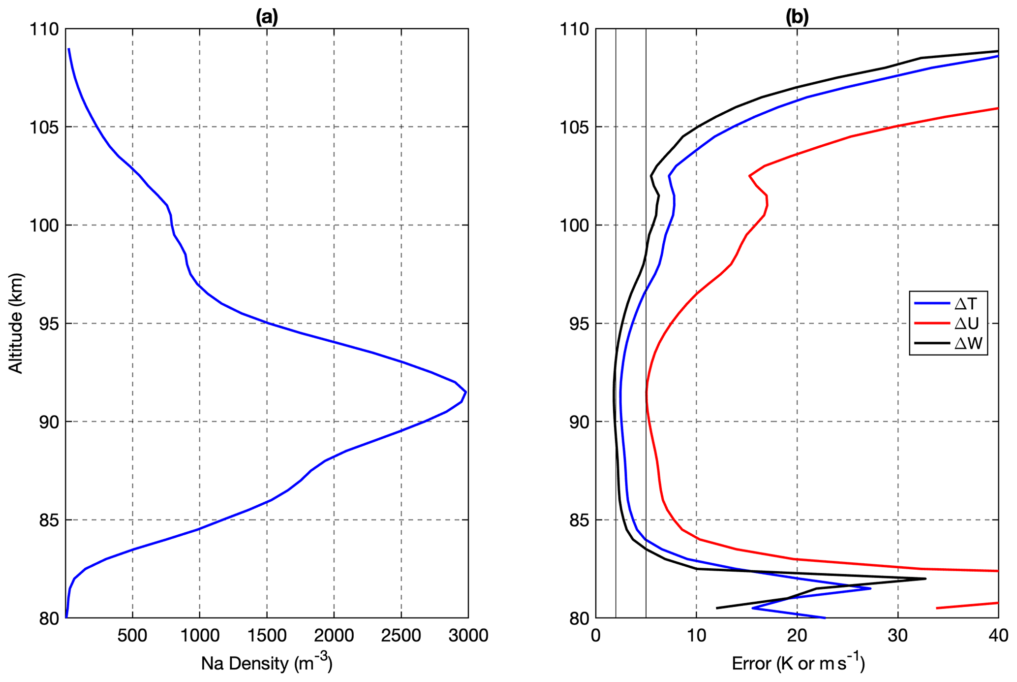
Figure A1 Panel (a) shows mean sodium density and (b) estimated uncertainties for temperature as well as horizontal and vertical winds.

Figure A2 Same as Fig. 4 but for horizontal and vertical winds.

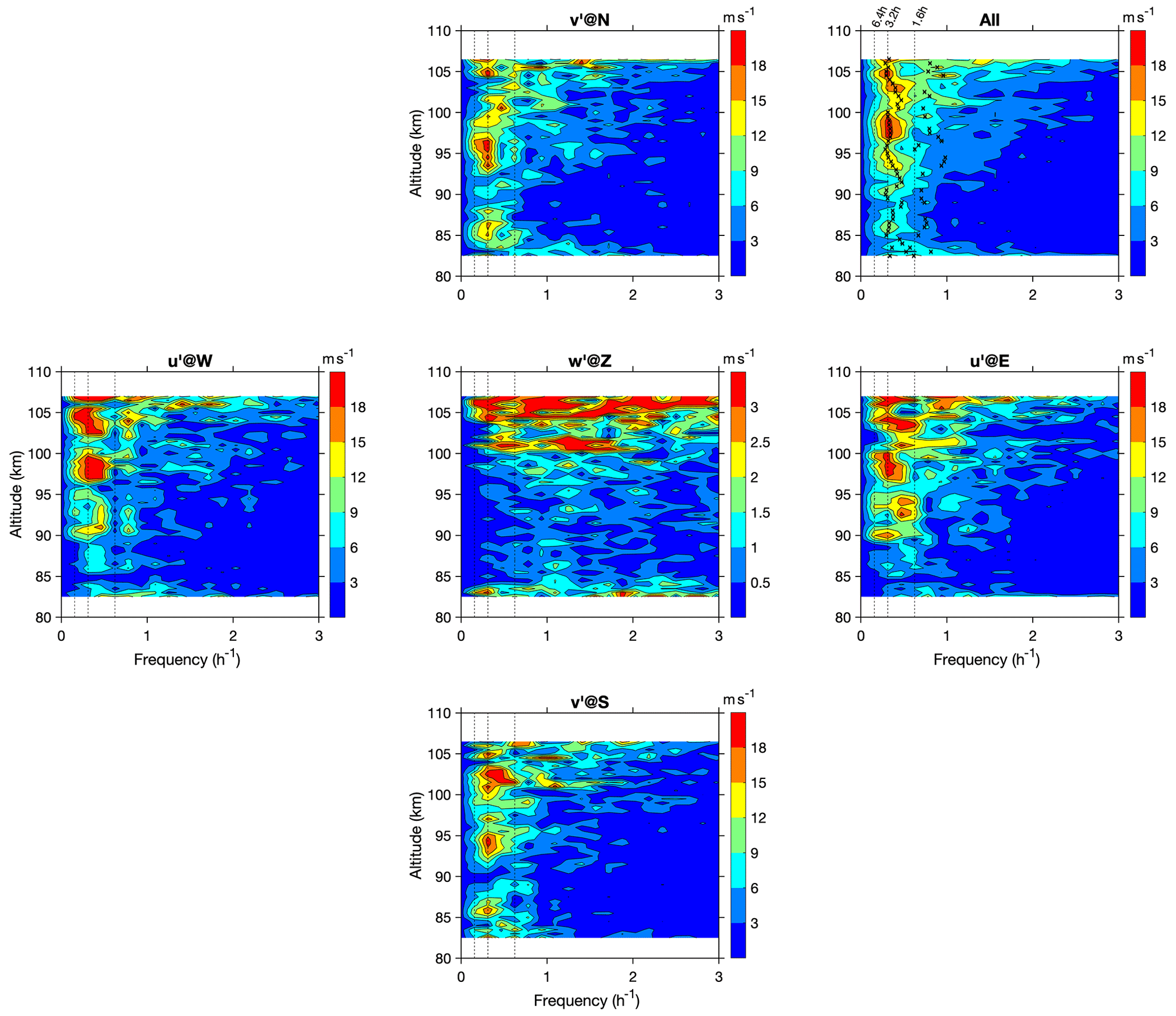
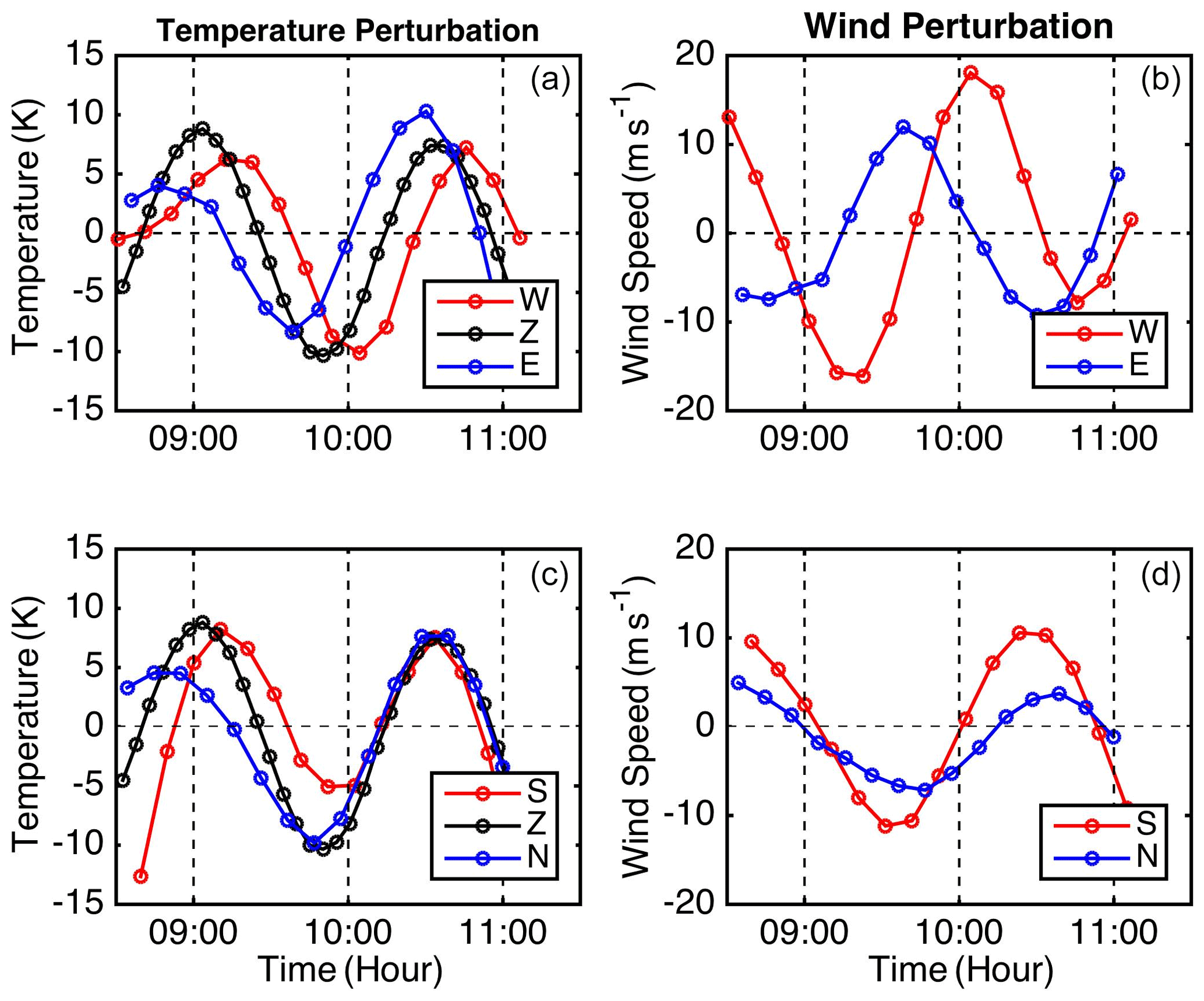
Figure A3 Filtered (a, c) temperature perturbation as well as (b) zonal and (d) meridional wind perturbations for the 1.6 h wave in different directions. Note that the circles indicate the raw measurements with 5.1 and 10.2 min temporal resolution as described in Sect. 2. No interpolation was applied to the data, so the filters applied on the time series are not exactly the same as described in the text, even though they have the same cut-off periods.

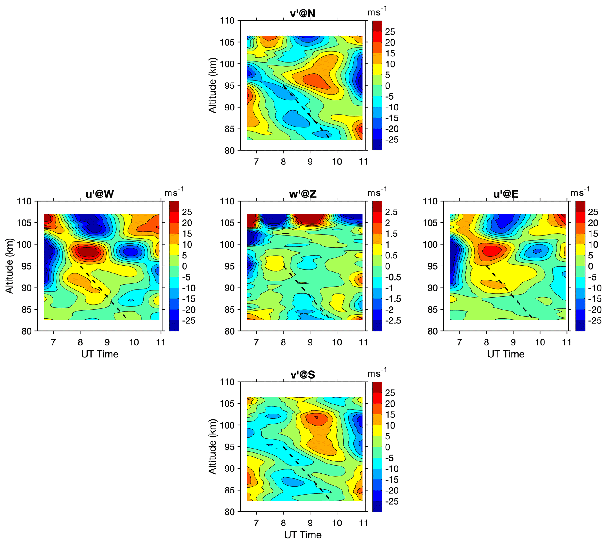
Figure A4 Same as Fig. 6 but for horizontal and vertical winds. Note that they are zonal winds at W and E, meridional winds at S and N, and vertical wind at Z.

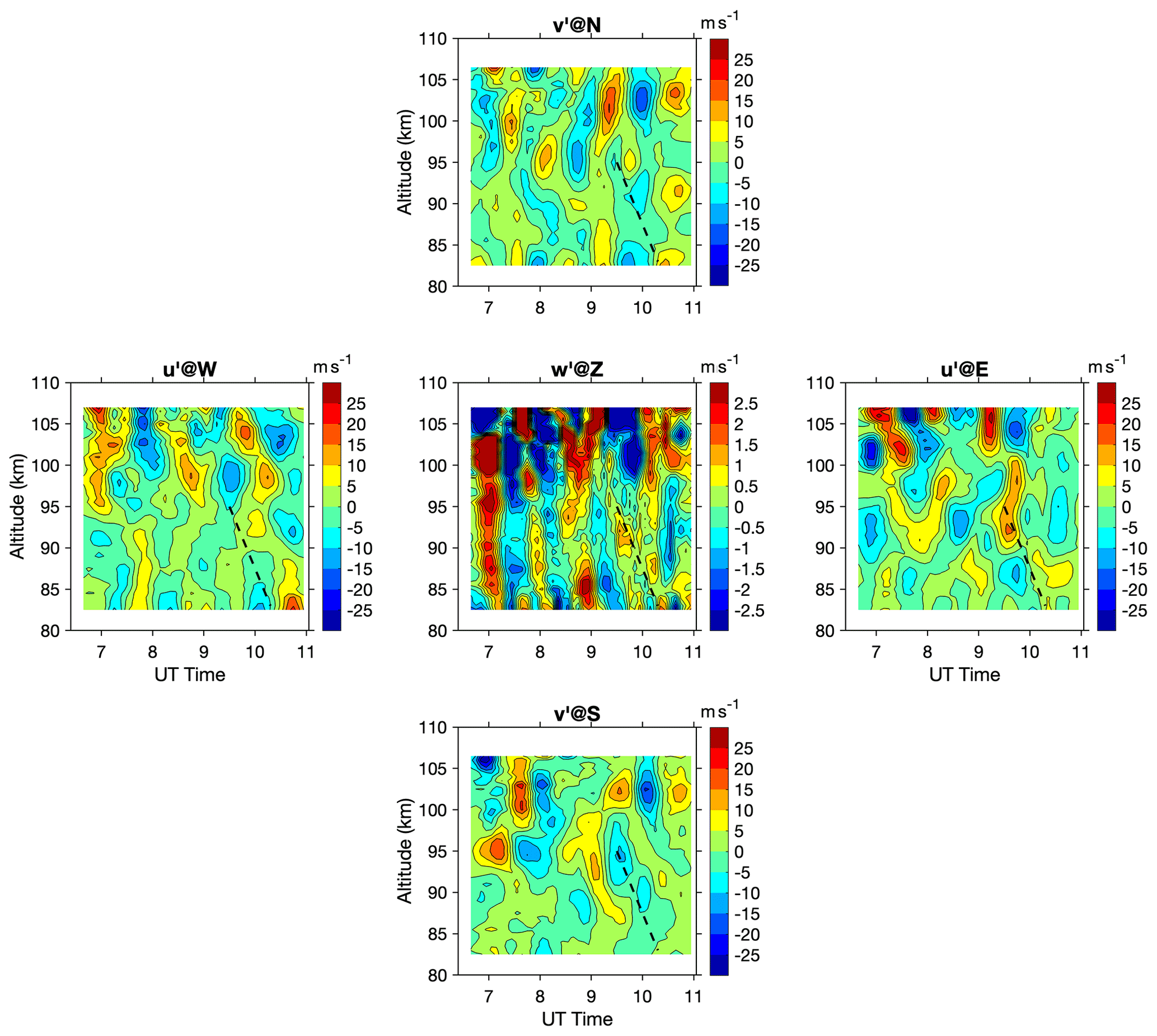
Figure A5 Same as Fig. 7 but for horizontal and vertical winds. Note that they are zonal winds at W and E, meridional winds at S and N, and vertical wind at Z.

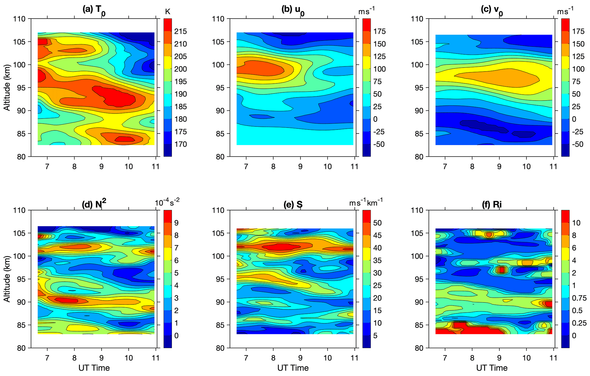
Figure A6 Same as Fig. 5 but the background contains all perturbations with periods longer than 2.2 h, which includes the quasi-3.2 h wave.

Figure A7 Same as Fig. 9 but calculated from the dispersion relation defined by Eq. 10.

Figure A8 Same as Fig. 9 but calculated from the dispersion relation defined by Eq. 11.