Measurement uncertainties of scanning microwave radiometers and their influence on temperature profiling

In order to improve observations of the atmospheric boundary layer (ABL), the European Meteorological Network, EUMETNET, and the Aerosol, Clouds, and Trace Gases Research Infrastructure, ACTRIS, are currently working on building networks of microwave radiometers (MWRs). Elevation-scanning MWRs are well suited to obtain temperature profiles of the atmosphere, especially within the ABL. Understanding and assessing measurement uncertainties of state-of-the-art scanning MWRs is therefore crucial for accurate temperature profiling. In this paper, we discuss measurement uncertainties due to the instrument setup and originating from external sources, namely (1) horizontal inhomogeneities of the atmosphere, (2) pointing errors or a tilt of the instrument, (3) physical obstacles in the line of sight of the instrument, and (4) radio frequency interference (RFI). Horizontal inhomogeneities from observations at the Jülich Observatory for Cloud Evolution (JOYCE) are shown to have a small impact on retrieved temperature profiles ($<\left|\mathrm{0.22}\mathrm{K}\right|$ in the 25th and 75th percentiles below 3000 m). Typical instrument tilts, that could be caused by uncertainties during the instrument setup, also have a very small impact on temperature profiles and are smaller than 0.1 K below 3000 m for up to 1^∘ of tilt. Physical obstacles at ambient temperatures and in the line of sight and filling the complete beam of the MWR at the lowest elevation angle of 5.4^∘ have to be at least 600 m away from the instrument in order to have an impact of less than 0.1 K on obtained temperature profiles. If the obstacle is 5 K warmer than its surroundings then the obstacle should be at least 2700 m away. Finally, we present an approach on how to detect RFI with an MWR with azimuth and elevation-scanning capabilities. In this study, we detect RFIs in a water vapor channel that does not influence temperature retrievals but would be relevant if the MWR were used to detect horizontal humidity inhomogeneities.

1 Introduction and motivation

The atmospheric boundary layer (ABL) is a crucial, yet often under-sampled, part of the atmosphere. ABL monitoring is important for the short-range forecasting of severe weather. Top-priority atmospheric variables for numerical weather prediction (NWP) applications, like temperature (T) and humidity (H) profiles, are currently not adequately measured (Teixeira et al., 2021). Ground-based microwave radiometers (MWRs) like HATPRO (Humidity And Temperature PROfiler) are well suited to obtain such T profiles in the ABL as well as coarse-resolution H profiles because they provide continuous and unattended observations in nearly all weather conditions (Liljegren, 2002; Rose et al., 2005; Cimini et al., 2011; Löhnert and Maier, 2012). Besides zenith observations, which provide path-integrated values like integrated water vapor (IWV) and liquid water path (LWP) with a high temporal resolution (up to 1 s), elevation scans are used to retrieve more precise temperature profiles in the ABL (Crewell and Löhnert, 2007) as well as to assess horizontal inhomogeneities in water vapor and cloud coverage (Marke et al., 2020). It has been shown by previous studies that the assimilation of MWR observations is beneficial for NWP models; however, such observations are not yet routinely assimilated into any operational NWP model (De Angelis et al., 2016; Caumont et al., 2016).

Building an operational network of state-of-the-art MWRs is important to improve meteorological observations and is currently a goal which is pursued by several initiatives. The EU COST Action CA 18235 PROBE¹ (PROfiling the atmospheric Boundary layer at European scale) and the European Research Infrastructure for the observation of Aerosol, Clouds, and Trace gases (ACTRIS² currently focus on establishing continent-wide quality and observation standards for MWR networks for research as well as for NWP applications. Also, driven by the E-PROFILE³ program, a business case proposal was recently accepted by EUMETNET⁴ to continuously provide MWR data to the European meteorological services (Rüfenacht et al., 2021). The German Weather Service also investigates the potential of MWR networks for improving short-term weather forecasts over Germany. For all that, it is crucial to assess the uncertainties of state-of-the-art MWRs, as there is no comprehensive analysis and overview of uncertainties of these newest instruments yet. This study analyzes measurement uncertainties by external sources, but uncertainties also encompass instrument uncertainties like biases, drifts, random noise, and calibration errors, which have been partly discussed in previous studies (Liljegren, 2002; Crewell and Löhnert, 2003; Maschwitz et al., 2013; Küchler et al., 2016) but are in need of updating.

When installing an MWR, it has to be kept in mind that instrument setup, physical obstacles, and radio frequency interference (RFI) can have an impact on observations and the quality of the obtained atmospheric profiles. Therefore, identifying and coping with these kinds of errors is one important part of the quality control process, especially while searching for a suitable measurement location with minimum disturbances. For example, if physical obstacles like trees, towers, masts, walls, and mountains are too close to the MWR, they can have significant repercussions on elevation scans, which are necessary for deriving accurate T profiles (see Fig. 1 in Sect. 3.2 for more details on the benefit of elevation scans). That is why it is crucial to pinpoint the exact location of these obstacles and to determine a minimum distance at which they do not interfere with the MWR anymore.

This study will first introduce the newest Generation 5 HATPRO MWR in short in Sect. 2 and then describe the methods used like the forward model and retrieval model in Sect. 3, which are needed to assess measurement uncertainties. The main part of Sect. 4 will present a sensitivity study, which uses a line-by-line radiative transfer (RT) model in which beam-filling obstacles at any distance from the profiler can be simulated. Focusing on the V-band (50–60 GHz frequency range employed for temperature profiling), output comparisons with and without these simulated obstacles provide a theoretical atmospheric penetration depth per frequency channel and elevation. The impact of obstacles on T-profile retrievals will be shown as well. Other measurement uncertainties – like horizontal inhomogeneities in the ABL, pointing errors or tilts of the radiometer, and examples of RFI – and their ramifications will also be presented and analyzed.

2 HATPRO microwave radiometer

The instruments used in this study are HATPROs (Humidity And Temperature PROfilers), which are the most widely used MWRs within Europe⁵ and are manufactured by RPG-Radiometer Physics GmbH in Germany. These passive ground-based microwave radiometers operate within the K-band and V-band spectra (the 22–32 GHz water vapor absorption line and the 51–58 GHz oxygen absorption complex) and are among the best radiometers to obtain T profiles and coarse H profiles of the troposphere. HATPROs measure microwave radiances expressed as brightness temperatures (T_B) in 14 different frequency channels (see Table 1) in parallel, in zenith, and in other elevation angles, with a temporal resolution on the order of seconds. The T_Bs can be used to retrieve the T profiles and H profiles but also path-integrated values, like integrated water vapor (IWV) and liquid water path (LWP), with uncertainties below 0.5 kg m⁻² and 20 g m⁻², respectively (Löhnert and Crewell, 2003). The quality of these retrievals naturally depends on how well they were trained and implemented. Retrieving T profiles within the ABL works best when using elevation scans. That is why HATPROs measure at multiple elevations, usually using between 6 and 10 different angles between 0 and 90^∘. Elevation scans, although conducted with all frequency channels, are usually only used within the V-band, as the channels there are optically thick, especially channels 10–14. That means that penetration depth in these channels is low enough to ensure measurement benefits for resolving the temperature profile when using different elevation angles (see Sect. 4.3 and Table 2 for more details on penetration depths or maximum detection distances).

Table 1 Center frequencies, bandwidths, and half-power beam widths (HPBWs) of the 14 HATPRO channels (RPG-Radiometer Physics GmbH, 2015).

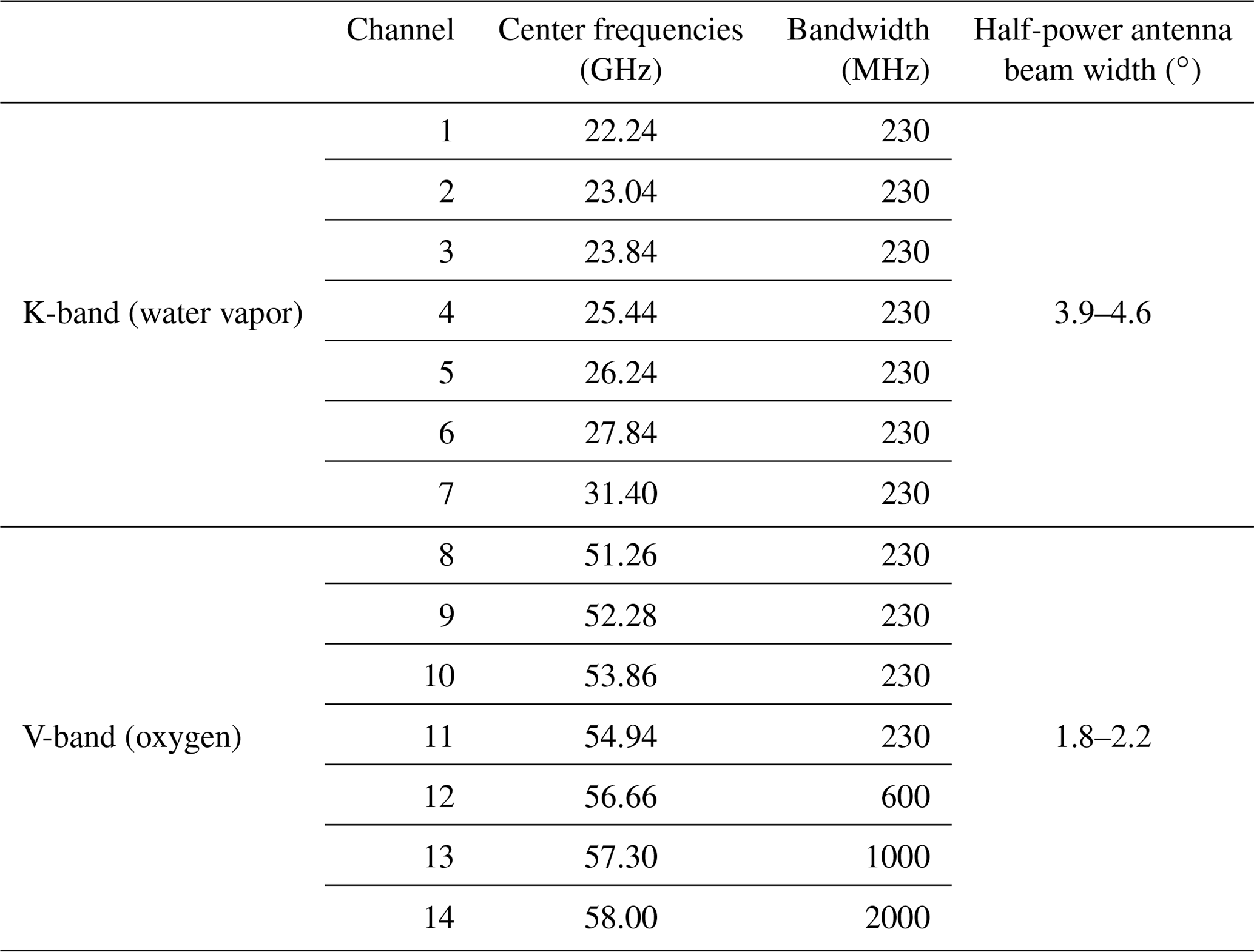
T_B accuracy is different for each channel and is usually below 0.5 K for Generation 5 HATPROs, according to the manufacturer, RPG-Radiometer Physics GmbH. This accuracy mainly consists of these four instrument errors, which are not the topic of this study: calibration repeatability, radiometric noise, drift, and bias (Crewell and Löhnert, 2003; Maschwitz et al., 2013; Küchler et al., 2016). Other radiometer characteristics like antenna beam width and receiver bandwidth (as well as atmospheric propagation) can also have an impact on scanning MWR measurements, depending on the frequency channel and elevation angle (Han and Westwater, 2000; Meunier et al., 2013). However, within the V-band and the elevation angles used in this study (>4^∘), these impacts are negligibly small (<0.05 K) (Meunier et al., 2013), also considering that the half-power antenna beam width (HPBW) of a HATPRO within the V-band is only up to 2.2^∘ (RPG-Radiometer Physics GmbH, 2015), and the penetration depths of the V-band channels are limited. Additional sources of uncertainty for HATPRO products are due to radiative transfer model and absorption coefficient errors (see Sect. 3).

3 Methods

Here, we describe the most important methods used for analyzing measurement uncertainties and their influence on T profiling, especially the methods needed for the simulation of pointing errors and the simulation of physical obstacles. Measurement setups required for measuring horizontal inhomogeneities and identifying RFIs, as well as finer details in the simulations of obstacles and pointing errors, are described in the “Results and discussion” section (Sect. 4) as needed.

3.1 Forward model

In this study, non-scattering radiative transfer simulations are carried out based on Simmer (1994). Gaseous absorption is calculated according to Rosenkranz (1998), whereby the water vapor continuum is modified according to Turner et al. (2009), and the 22 GHz water vapor line width is modified according to Liljegren et al. (2005). This model depicts the energy transfer in the form of electromagnetic radiation through the atmosphere via absorption and emission by gas molecules, and it is modified here to simulate physical obstacles at different distances and elevation angles and to assess pointing errors in a cloud-free atmosphere.

The input to the model consists of radiosonde profile data from the Richard Aßmann Observatory (RAO) in Lindenberg, Germany, from the year 2000 which provide pressure, height, temperature, and relative humidity. There were four soundings per day and in total 1436 usable soundings for the year 2000. The provided height levels from the atmospheric soundings were linearly interpolated to a spacing of 1 m below 150 m, 10 m below 10 km, and 1000 m below 30 km. When there were no data available above certain heights (mostly between 10 and 30 km), the gaps were filled with data from the International Standard Atmosphere (ISA) at mid-latitude⁶. The forward model uses the same height levels as the interpolated soundings. Input parameters include the 14 HATPRO frequency channels and the used elevation angles (5.4, 10.2, 19.2, 30, 42, and 90^∘). For the most part of this study, the focus lies on the seven V-band channels, as only these are needed to later retrieve T profiles (see Sect. 3.2).

Within this non-scattering RT model, the calculation of the optical thickness τ of the atmosphere plays an important role. It is dimensionless and calculated via the integration of the gas absorption coefficient β_a over the optical path s^′:

$$\begin{array}{}\text{(1)}& \mathit{\tau }(s,\mathit{\nu })={\int }_{\mathrm{0}}^s{\mathit{\beta }}_a\left(s^{\prime },\mathit{\nu }\right)\mathrm{d}{s}^{\prime }.\end{array}$$

τ is not only dependent on the total optical path s but also on the frequency ν. First, τ is calculated in the zenith direction. By multiplying the zenith τ by $\mathrm{1}/\cos \left(\mathit{\theta }\right)$, with θ being the zenith angle, we arrive at the optical depth at any arbitrary elevation angle assuming horizontal homogeneity. In order to simulate physical obstacles, the optical thickness τ can be manually set to very high values (e.g., τ=100) at the desired height level and in turn the desired distance for any elevation angle. Doing this will ensure that no radiation beyond the simulated obstacle will pass through to the radiometer position. Without further modifications, the obstacles will have the ambient temperature of their surroundings derived from the radiosonde input. Within this study, the influence of “heated” obstacles with +5 K compared to ambient temperatures has also been analyzed. Such heated obstacles could, for example, represent facades of buildings or mountain slopes which are lit by the sun.

For the simulation of obstacles, some assumptions were made: (1) horizontal homogeneity of the atmosphere is required, (2) the obstacle is a perfect blackbody with ambient (or +5 K) temperature, and (3) the whole cone from the antenna HPBW is filled with the obstacle. As an example, for an antenna beam width of 3^∘, the radius of the cone is about 13.1 m when 500 m away from the radiometer and about 26.2 m when 1000 m away.

As the forward model should simulate T_B measurements from an MWR, radiometric white Gaussian noise of 0.5 K was added to all seven V-band channels.

3.2 Retrieval model

With the help of a retrieval model or algorithm, we can calculate a response of retrieved atmospheric parameters like T profiles to the T_B measurement uncertainties from obstacles, pointing errors, or horizontal inhomogeneities. The temperature retrieval itself is trained and tested with years of radiosonde data from a certain location, in our case, from near or the same locations where the measured or simulated T_Bs are gained. In the analysis of horizontal inhomogeneities (Sect. 4.1), retrieval coefficients derived from De Bilt in the Netherlands were utilized. De Bilt was chosen due to its climatological similarity to JOYCE in Jülich, where all the measurements were conducted, and because it was the nearest place where retrieval coefficients were available. Conversely, when examining simulated pointing errors (Sect. 4.2) and the influence of obstacles (Sect. 4.3), retrieval coefficients from RAO in Lindenberg were employed. RAO in Lindenberg was selected because it provided a substantial dataset of radiosonde data spanning multiple years, enabling statistical analysis. Likewise, these radiosonde data are already utilized as inputs in the forward model. The applied coefficients of this retrieval model incorporate absorption and emission from liquid water (Liebe et al., 1993), in addition to water vapor and oxygen.

Retrieval coefficients are generated through multi-variate linear regressions. These coefficients are needed to calculate T profiles from T_Bs as seen in Eq. (2),

$$\begin{array}{}\text{(2)}& T_z=d_{\mathrm{0}}+\sum _{\mathit{\nu }}\sum _{\mathit{\theta }}{d}_{\mathrm{1}\mathit{\nu }\mathit{\theta }}{T}_{\mathrm{B}\mathit{\nu }\mathit{\theta }},\end{array}$$

where d₀ is the offset value, d_1νθ are the regression coefficients, z is the index for each output layer height, and ν and θ stand for frequency and elevation angle, respectively (Crewell and Löhnert, 2007; Meunier et al., 2013). This T-profile retrieval takes the used frequency channels and elevation angles into account. In this study, the channels from the V-band are 8–14, and the six elevation angles are 5.4, 10.2, 19.2, 30, 42, and 90^∘. However, channels 8–10 are only used at 90^∘ elevation, while channels 11–14 are used at all six elevation angles. Another approach constitutes less precise zenith-only T-profile retrievals, which only take frequency into account and which are calculated as seen in Eq. (3):

$$\begin{array}{}\text{(3)}& T_z=c_{\mathrm{0}}+\sum _{\mathit{\nu }}\left(c_{\mathrm{1}\mathit{\nu }}{T}_{\mathrm{B}\mathit{\nu }}+c_{\mathrm{2}\mathit{\nu }}{T}_{\mathrm{B}\mathit{\nu }}^{\mathrm{2}}\right).\end{array}$$

Here, c₀ is the temperature offset, and the regression coefficients are c_1ν and c_2ν. There is an added quadratic term compared to Eq. (2), which helps improve the retrieval accuracy for zenith-only observations. Both retrievals output temperature at 43 height levels, from the surface up to 10 km height, with a higher vertical spacing in the lower 5 km.

The improvement of temperature profile precision using elevation scans compared to zenith-only observations can be seen in Fig. 1. Therefore, it is strongly advised to use elevation scanning when possible. T-profile retrievals which make use of elevation scans have a higher precision within the whole lower troposphere than T-profile retrievals using only zenith measurements, with a difference in standard deviation of around 0.5 K between 200 and 1000 m and around 0.2 K between 1000 and 5000 m.

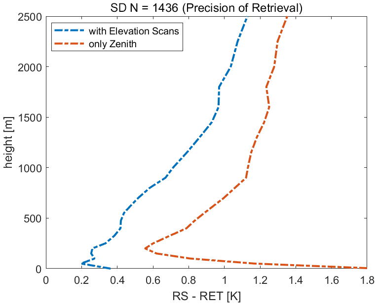
Figure 1 Precision of retrievals which make use of elevation scans (blue line, with six elevation angles) versus retrievals which only use zenith measurements (red line). Shown are the standard deviations (SDs) of the mean differences of T profiles from radiosondes (RSs) and the retrieved T profiles (RET) from forward modeled T_Bs from these radiosondes (T profiles from radiosondes minus retrieval). These were calculated from 1436 radiosondes from the year 2000 at RAO.

4 Results and discussion

Here, measurement uncertainties of scanning HATPRO microwave radiometers are shown and discussed in detail. These include horizontal inhomogeneities of the atmosphere (measured), pointing errors caused by a tilt of the instrument (simulated), the influence of physical obstacles in the line of sight of the instrument (simulated), and examples of RFIs and how to identify them (measured).

4.1 Horizontal inhomogeneities

One of the assumptions for the elevation retrieval to work properly is the horizontal homogeneity of the atmosphere. In reality, however, horizontal homogeneity is not always given. In order to investigate the impact of real-world horizontal inhomogeneities on retrieved T profiles, 3-week MWR measurements from JOYCE (Löhnert et al., 2015) from August to September 2022 are analyzed. The HATPRO was measuring at multiple elevation angles (5.4, 10.2, 19.2, 30, 42, and 90^∘) to the north and – immediately after the completion of such an elevation scan – did the same to the south. This scan pattern was repeated roughly every 15 min (the duration of one scan is roughly 2.5 min). To exclude the influence of clouds when needed during analysis, clear-sky profiles were considered by filtering out cases with a LWP >10 g m⁻² (for about a 30 min period before and after a scan).

4.1.1 T_B analysis

For the analysis, every pair of north-facing scans and immediately following south-facing scans is compared. The mean T_B difference over all north- and south-facing measurement pairs as a function of the V-band channel and elevation and their standard deviation are presented in Fig. 2 for clear-sky only and clear-sky and cloudy conditions. The standard deviations – minus the corresponding radiometric noise of the T_B measurements – and thus the variability of the T_B differences are an indicator of actual measured horizontal inhomogeneities, while the mean differences, in contrast, can also be the consequence of other factors. Keep in mind that the radiometric noise for Generation 5 HATPROs is on average 0.15 K within the V-band, according to the manufacturer (RPG-Radiometer Physics GmbH, 2015), with slightly higher values in the optically thinner channels 8–10 and slightly lower values for channels 11–14.

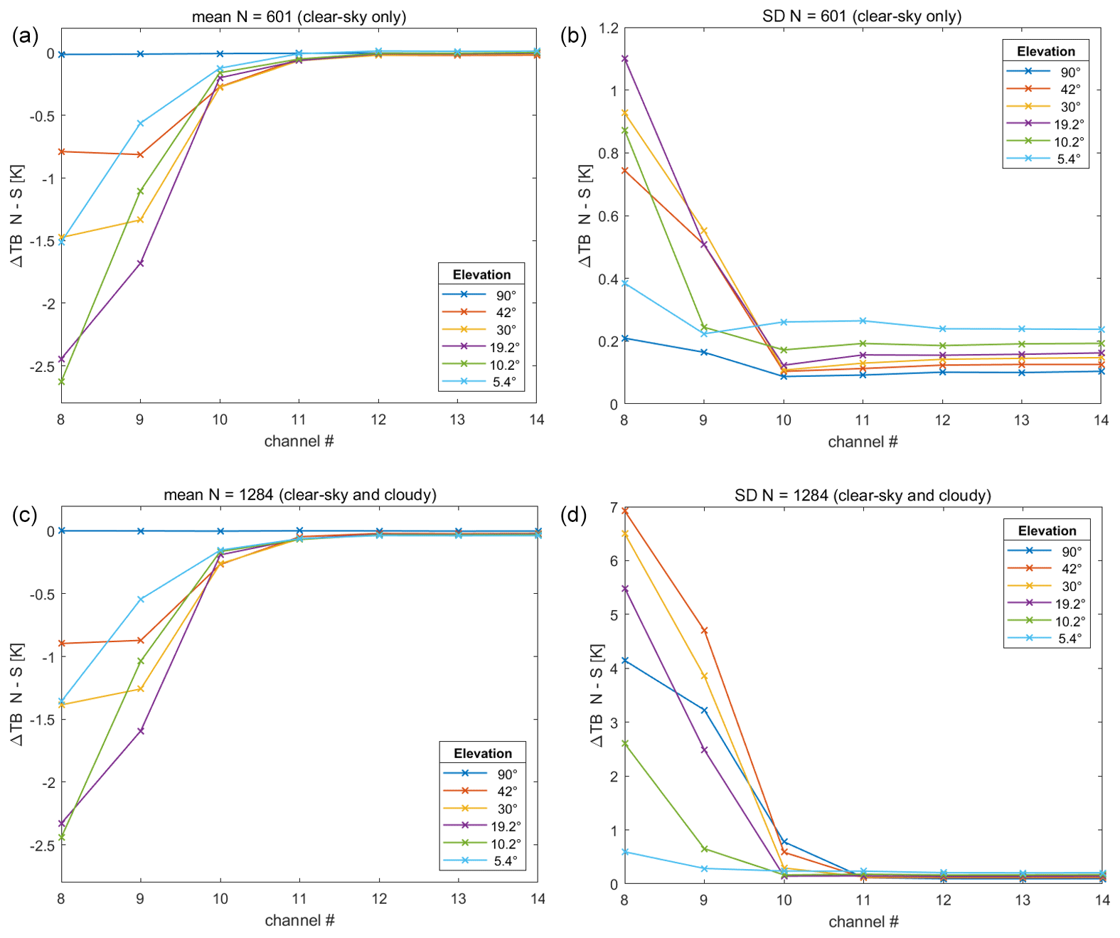
Figure 2 T_B differences from north- and south-facing radiometer measurements over a 3-week period in summer 2022 from JOYCE from clear-sky only (a, b) and clear and cloudy conditions (c, d). On the left are the mean differences per V-band channel and elevation, on the right the corresponding standard deviations (SDs). Note that the y axes for the standard deviation plots are not the same.

Let us first focus on the optically thinnest channels of the V-band, channels 8–9. These channels reach the deepest penetration depths and show the highest mean differences in north- and south-facing measurements and also the highest standard deviations of the T_B differences in all elevations. This is in line with expectations considering the usually highly inhomogeneous distribution of water vapor to which channels 8–9 (and to a lesser extent channel 10) are sensitive, along with temperature variability (Westwater et al., 2005).

Standard deviations of T_B differences in channels 8 and 9 show values of up to 1.1 K at 19.2^∘ elevation in clear-sky conditions and up to 6.9 K at 42^∘ elevation, when cloudy conditions are included. Higher absolute standard deviations for cloudy conditions are to be expected in those channels, as horizontal inhomogeneities increase when a cloud is present in one scan but not in the corresponding scan in the opposite direction. As the occurrence probability of clouds decreases towards the surface, standard deviations relative to higher elevations are lower for lower elevations when cloudy conditions are included. The increasing optical depth in channels 8–9 at lower elevations is also a reason for these observed lower standard deviations in relation to the higher elevation angles. The standard deviation at 90^∘ elevation in channels 8–9 can be explained by the fact that – although at zenith both north- and south-facing scans are pointing in the exact same direction – the measured variability here is not due to horizontal inhomogeneities but rather due to the noise of the instrument and the 2.5 min time difference between a north- and a south-facing scan, in which atmospheric variables could have changed slightly.

The mean absolute differences in channels 8 and 9 for all the elevations vary from 0.6 K up to 2.6 K and are fairly similar for clear-sky only and clear-sky and cloudy conditions. Excluding zenith for now, the higher elevation angles in the optically thinner channels show, in general, lower mean absolute differences than the intermediate elevation angles because they cover a smaller horizontal area compared to the intermediate elevation angles. The small values in mean difference in the lowest elevation can be explained by the fact that here the measurements do not reach high enough into the atmosphere and that water vapor and cloud inhomogeneities do not have much of an impact on these channels.

As for the optically thicker channels 11–14, they show much lower mean differences and standard deviations ($<\mathrm{0.06}\pm \mathrm{0.26}$ K for clear-sky and $<\mathrm{0.06}\pm \mathrm{0.23}$ K including cloudy conditions) than for channels 8–10, as they do not penetrate the atmosphere very deeply. Lower elevations at optically thicker channels show higher standard deviations because they cover a larger horizontal area than higher elevations and are thus subject to higher near-surface temperature variability, which is also more pronounced during clear-sky conditions.

The obtained mean differences seen in Fig. 2 imply that T_B values in the south are consistently higher than in the north for the 3-week measurement period, independent of clear-sky or cloudy conditions. Additional forward model simulations for horizontal inhomogeneities – in which humidity profiles from RAO radiosondes were altered – reveal that an average difference of about ΔIWV≈ 3.4 kg m⁻² in a south–north direction in a clear-sky scenario would be necessary in order to achieve similar mean T_B differences as seen in Fig. 2. Such a large average difference in IWV as a consequence of horizontal inhomogeneity is highly unlikely. That is why a pointing error caused by a tilt of the instrument is most probably the main reason for these observed mean differences. Via forward model simulations with different elevation angles including simulated instrument tilts, we found similar patterns as seen in Fig. 2 when assuming a tilt of 0.6^∘ in a south–north direction (see Sect. 4.2 and Fig. 4, and compare with Fig. 2). While complex geography around the measurement site and general weather conditions can also have an influence on the mean difference in measured T_Bs, their expected mean impact is significantly smaller than what is depicted in Fig. 2. There is a slight mean diurnal cycle of the mean differences (maximum change of mean difference during night and day for channel 8 at 5.4^∘ elevation compared to the mean differences in Fig. 2 is smaller than ±0.2 K; all other V-band channel and elevation combinations are smaller than this), which means the influence of the daily variation of weather is rather low compared to the overall impact of tilt but not absent.

4.1.2 T-profile analysis

When retrieving a T profile by means of an MWR scan, only zenith measurements are used for channels 8–10, whereas all available elevation angles (including zenith) are used for channels 11–14. That is the reason why the impact of horizontal inhomogeneities on retrieved T profiles is rather small, even though off-zenith mean T_B differences in channel 8–9 can be as high as 2.6 K in our examples. This small impact can be seen in Fig. 3, where the median T-profile differences retrieved from the north-facing and south-facing scans are shown. The percentiles in Fig. 3 represent actual horizontal inhomogeneities and/or variabilities of the atmosphere, while the medians are a consequence of the assumed tilt of the instrument. The absolute median difference up to 3000 m is always below 0.08 K (0.05 K for clear-sky). The 25th and 75th percentiles do not exceed −0.20 and 0.22 K, respectively, and only come close to these values near the surface where the variability is the highest. The 5th and 95th percentiles show a similar pattern and do not exceed −0.8 and 0.8 K near the surface. It is evident from Fig. 3 that variability near the surface is higher in clear-sky-only conditions, when compared to conditions including clouds. This peculiarity can be explained by two reasons. Firstly, different types of surfaces around the measurement site (e.g., concrete vs. grass and trees) heat up differently when the sun is shining than when there are very cloudy conditions where heat is more evenly distributed near the surface. This heat is dispensed to the air near the surface where especially the optically thicker channels pick it up. Secondly, inversions near the surface during cloudy conditions are less likely than during clear-sky, which also leads to less variability near the surface during cloudy conditions. Overall, the medians and 25th and 75th percentiles in all conditions lie within the expected uncertainty of HATPRO temperature profiles (Löhnert and Maier, 2012).

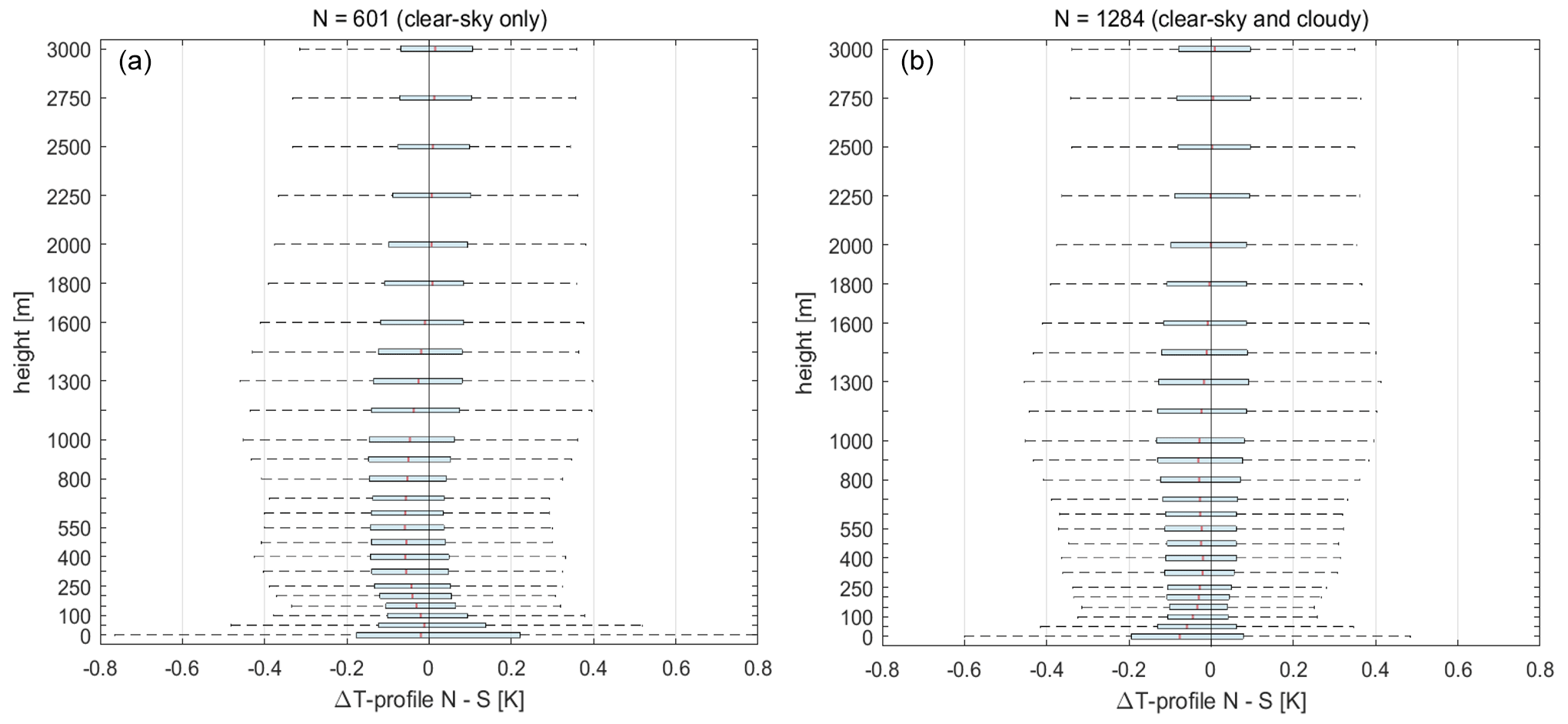
Figure 3 Differences in derived T profiles at certain heights from northward and southward elevation scans at JOYCE. The red lines are the medians from a 3-week period in late summer 2022, and the horizontal bars show the 25th and 75th percentiles, while the dashed lines show the 5th and 95th percentiles. (a) Only clear-sky conditions are shown and (b) clear and cloudy conditions.

4.2 Pointing errors or tilts

As discussed in Sect. 4.1, measured mean T_B differences from elevation scans in opposing directions can be caused by pointing errors, not only by actual horizontal inhomogeneities of the atmosphere. Pointing errors are errors that arise from a tilt of the radiometer and are usually the result of an improper setup by the operator but can also be due to internal instrument misalignments. They impact all elevation and zenith measurements. For 30^∘ elevation scans for example, a 1^∘ tilt of the instrument to the south will lead to a measurement at 29^∘ facing south and 31^∘ facing north. Tilts have a smaller impact at higher elevations and zenith observations than on lower ones (due to trigonometric reasons). A tilt of more than 2^∘ can have very significant repercussions on T_B measurements at the lowest elevation angle of 5.4^∘, as the half-power antenna beam width of a HATPRO is up to 2.2^∘ in the V-band, and therefore emissions from the surface will interfere more and more, the lower the elevation scans reach down.

4.2.1 T_B analysis

Figure 4 shows the simulated impact on T_B measurements for different elevations when there is a pointing error of 0.6^∘ (in opposing directions, e.g., in a south–north direction). Depicted are differences of simulated T_B measurements from an MWR with and without tilt in an inversion-free atmosphere (e.g., International Standard Atmosphere – ISA). When focusing on the V-band channels, we can spot that the presence of a 0.6^∘ pointing error yields the exact same pattern and almost the same values of ΔT_Bs as seen in Fig. 2a and c. From this, we conclude that the systematic differences from north- and south-facing scans in Sect. 4.1 are actually – for the most part – the result of a slightly misaligned MWR. Due to the fact that the inhomogeneities were analyzed by the difference of north- and south-facing scans, a real-world misalignment or tilt of the MWR of only 0.3^∘ in a south–north direction (e.g., such a 0.3^∘ tilt at 30^∘ elevation leads to 30.3^∘ elevation in the north and to 29.7^∘ elevation in the south, which makes a 0.6^∘ pointing difference) would be enough to produce these particular ΔT_B patterns and values as depicted in Fig. 4. For the optically thinner K-band channels, a tilt can have an even larger influence on T_B measurements, especially at lower elevations. As far as T profiling is concerned, K-band channels are not used at all, and V-band channels 8–10 are only used in zenith, therefore diminishing the influence of tilts or pointing errors on T profiling.

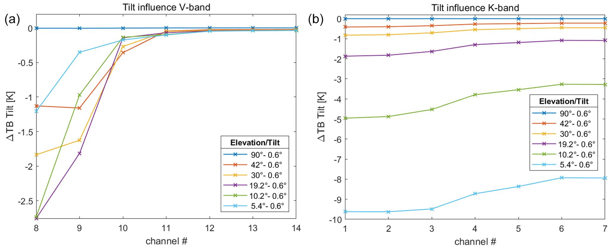
Figure 4 Influence of tilt on T_B measurements for elevation scans within the V-band (a) and the K-band (b). Depicted are simulated T_B measurement differences in an inversion-free ABL from a non-tilted instrument and an instrument with 0.6^∘ tilt (non-tilted minus tilted).

When trying to analyze water vapor inhomogeneities with a full azimuth scan, e.g., at 30^∘ elevation, a pointing error of 0.6^∘ in a certain azimuth direction always has an impact of more than 0.4 K in all K-band channels (with up to 0.8 K in channel 1) when compared to measurements without tilt (see Fig. 4b). Even though measurements within the K-band are not a focus in this study, it may be noteworthy that – without going into much detail – this would directly translate to an impact on IWV of about ±0.24 kg m⁻² in the direction of the tilt when retrieving along the 30^∘ elevation path (measurements show that a 1 K T_B difference in channel 1 at zenith corresponds to a roughly 0.6 kg m⁻² change in IWV). Please also note that within the K-band, T_B uncertainties from receiver bandwidth and antenna beam width are also not negligibly small unlike in the V-band. For our HATPRO setup, they can vary between 0.1 and 0.3 K (Meunier et al., 2013).

4.2.2 T-profile analysis

Figure 5 shows the impact of pointing errors of up to ±1^∘ on T profiling when employing elevation scans. It depicts the T profile mean differences (bias at 0^∘ elevation) and their corresponding standard deviations from 1436 radiosondes from RAO over Lindenberg from the year 2000 and the retrieved profiles from simulated T_Bs from these radiosondes. For retrievals which make use of elevation scans, there is very little mean difference (between −0.13 and 0.24 K) in the lowest 1000 m, even when incorporating pointing errors of ±1^∘. Theses pointing errors hardly exceed ±0.1 K on the T profile when compared to a 0^∘ tilt. The precision of these T-profile retrievals is represented by the standard deviations, on which pointing errors of ±1^∘ have even less impact, as evident in Fig. 5. Standard deviations are roughly the same for all elevations and range from 0.20–0.45 K in the lowest 500 m and 0.45–1.15 K between 500 and 2500 m.

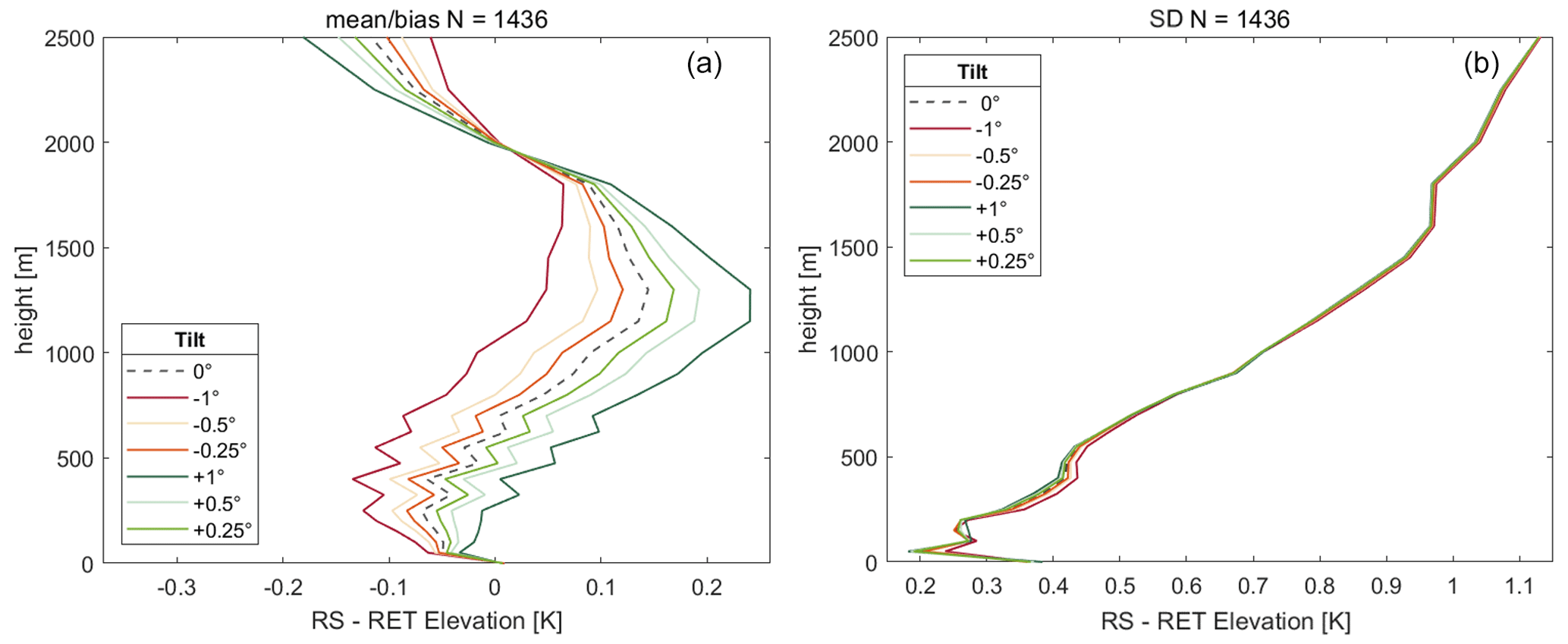
Figure 5 Mean differences (a) and their corresponding standard deviations (SDs) (b) of T profiles from radiosondes (RSs) over Lindenberg and the retrieved T profiles (RET) from forward modeled T_Bs from these radiosondes (T profiles from radiosondes minus retrieval). Retrievals make use of six elevation angles. Shown are the influences of tilts on the radiometer of up to ±1^∘. The mean values are calculated from 1436 radiosondes from the year 2000 from RAO.

For retrievals which only make use of zenith measurements, the impact of pointing errors on mean T_B differences and standard deviations is negligible, at least for smaller tilt angles below 2^∘. Nevertheless, T profiles which make use of elevation scans have a higher precision than T profiles derived from only zenith measurements, even if they are contaminated by pointing errors of up to ±1^∘ (compare the standard deviations from Fig. 5 with Fig. 1; the blue line in Fig. 1 corresponds to the content displayed in the right plot of Fig. 5, when there is no tilt).

In real-world scenarios, scanning on both sides of the radiometer – if possible – can mitigate pointing uncertainties to a certain degree, when T profiles are retrieved from the average of such scans. However, this approach comes with problems, such as longer measurement times, the assumption of horizontal homogeneity of the atmosphere, and the assumption that elevation scans on both sides even out linearly.

4.3 Influence of obstacles

When setting up an MWR at a new measurement location, it has to be kept in mind that external error sources like physical obstacles (e.g., trees, buildings, or nearby mountains) can have an impact on T_B measurements when they are too close and in the line of sight of the MWR, especially at lower elevation angles. The impact depends on the distance and temperature of the obstacle, as well as its size. When encountering a small or slim obstacle that does not fill the entire beam width of the instrument, the resulting impact is generally less significant compared to larger obstacles. Simulating obstacles that do not completely fill the beam width of the MWR (such as power lines or lightning rods) poses challenges. Therefore, in our simulations, we focus on beam-filling obstacles, for which a minimum distance can be determined at which they do not interfere with the measurements anymore. Our simulations of such beam-filling obstacles within the RT forward model have shown that, in general, the influence of obstacles on the measurements is the greatest within an inversion-free troposphere. The International Standard Atmosphere (ISA) can provide such an inversion-free example as an input. In order to simulate an obstacle, the optical thickness of the atmosphere within the RT model can be set to a very high value at the desired distance (see Sect. 3.1).

4.3.1 T_B analysis

Figure 6 shows the impact of beam-filling obstacles with ambient temperature on T_B measurements within the V-band in a mid-latitude standard atmosphere for certain elevation angles. The difference in T_B measurements with and without an obstacle tells us the exact impact of a certain obstacle. In general, the conducted simulations show that the impact of an obstacle is getting higher: (1) the nearer an obstacle is to the MWR, (2) the higher the elevation angle is, (3) the optically thinner the frequency channel is, and (4) the higher the temperature of the obstacle is compared to its surroundings.

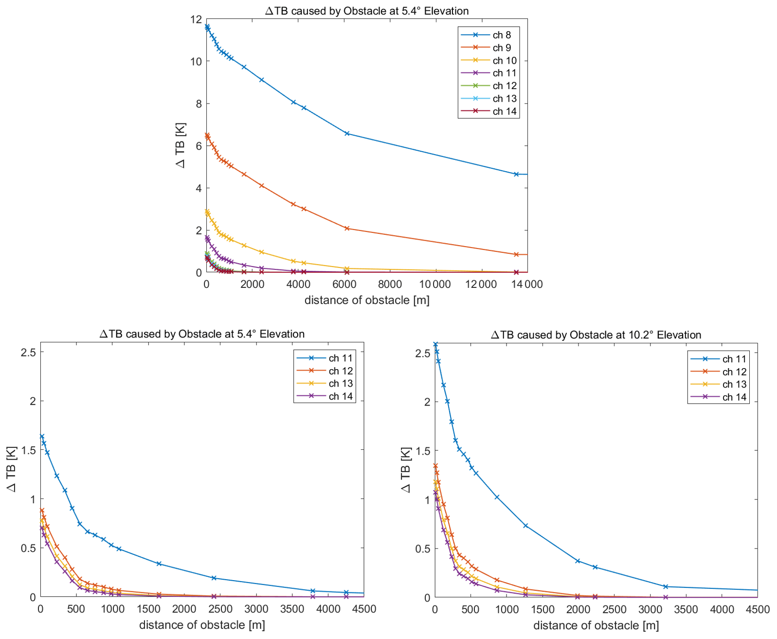
Figure 6 Impact of obstacles with ambient temperature on T_B measurements at different distances from the MWR in a standard atmosphere. Shown are the differences of T_Bs with and without an obstacle for elevation angles 5.4 and 10.2^∘ within the V-band. At the top for all V-band channels and at the bottom for channels 11–14.

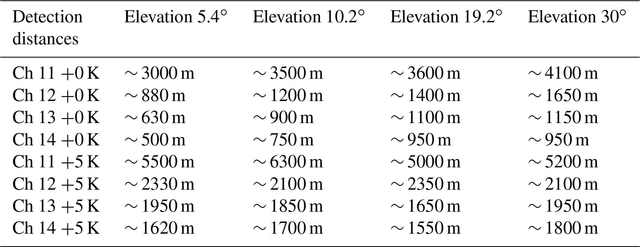
Channels 8 and 9 – which are the optically thinnest channels within the V-band – can reach far into the atmosphere, even at low elevations. They can detect obstacles at ambient temperature at the lowest elevation angle of 5.4^∘ from more than 30 km away. If we use a ΔT_B of ≤0.1 K as a detection threshold, channel 10 at the lowest elevation can still detect obstacles which are more than 10 km away. But as these channels are only used in zenith for T-profile retrievals, here we focus on channels 11–14. At 5.4^∘ elevation, channel 11 can detect ambient temperature obstacles from ∼ 3000 m away, while channels 12–14 have a detection range of 880 m to around 500 m. At 10.2^∘ elevation, these distances increase to ∼ 3500 m (for channel 11) and to 1200 m or 750 m (for channel 12–14), respectively. If an obstacle is warmer than its surroundings (e.g., 5 K warmer), the impact on T_B measurements and the detection distances will increase significantly. This maximum detection distance of obstacles is also a measure of penetration depth or how far the MWR can “see” into the atmosphere. A summary of these detection distances for different channel–angle combinations can be found in Table 2.

Table 2 Maximum detection distances of obstacles for different channel–angle combinations. A T_B detection threshold of 0.1 K is used. Values are given for beam-filling obstacles with ambient temperature and 5 K warmer.

During the course of a day or a year, atmospheric conditions change a lot, and an inversion-free troposphere/ABL is not always present, especially during winter nights. Temperature inversions near the surface, for example, can dampen the impact of obstacles, which can be derived from Fig. 7.

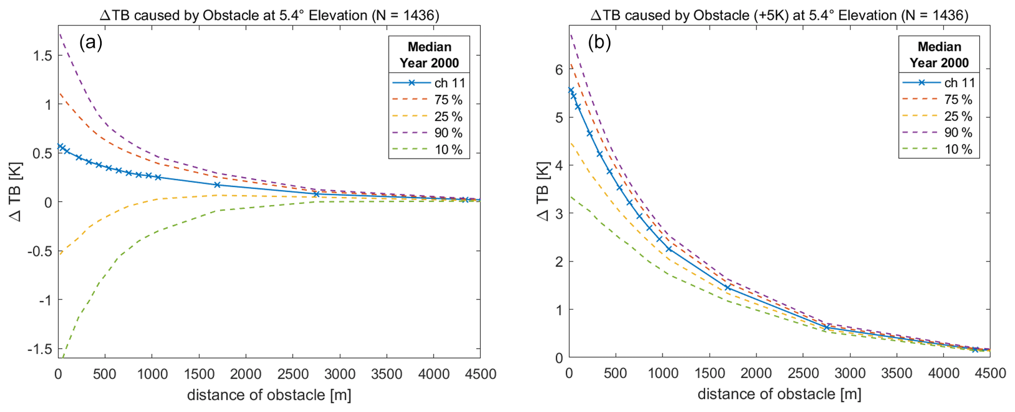
Figure 7 Statistics of T_B differences (obstacle in line of sight minus no obstacle) for channel 11 at 5.4^∘ elevation obtained from 1 year of Lindenberg radiosonde data. Bold line shows the median of the differences as a function of distance to obstacle and dashed lines the corresponding percentiles. (a) Obstacles have ambient temperature, and (b) obstacles are 5 K warmer than their surroundings.

Figure 7 depicts the impact of obstacles with different temperatures as a median of T_B differences (obstacle minus no obstacle) from the Lindenberg radiosonde data for the whole year 2000 at 5.4^∘ elevation for channel 11. This channel was chosen as an example because it shows the highest impact from channels 11–14. Looking at the 25th and 10th percentile lines, these indicate cases with inversions near the surface, while the 90th percentile line approximately represents the inversion-free scenario, as seen before in Fig. 6. For an ambient temperature obstacle, the ΔT_B can even become negative when there is an inversion, meaning that the ambient temperature obstacle near the colder surface blocks the MWR from observing warmer atmospheric layers above and beyond the obstacle. For an obstacle which is 5 K warmer than its surroundings, the impact on ΔT_B observations is significantly higher and will likely be positive, even when there are moderate inversions present near the surface.

4.3.2 T-profile analysis

Previously, the focus of our discussions has been on the influence of obstacles on T_B measurements. In the following, we will shift our attention to the influence of obstacles on retrieved T profiles. Simulations and retrievals have revealed that the average impact of obstacles on T profiles is strongest in inversion-free ABL cases. That is why the following results have been obtained in such inversion-free cases. Figure 8 shows the impact on T profiles from different beam-filling obstacles at certain distances to an MWR in a standard atmosphere. To minimize the impact of obstacles ($\le \left|\mathrm{0.1}\mathrm{K}\right|$), such as tall trees or nearby buildings, which possess ambient temperatures and are visible at an elevation of 5.4^∘, they must be situated at a distance of greater than 600 m (keep in mind that at 600 m distance an obstacle would need to be at least 57 m tall in order to block the line of sight of the MWR at 5.4^∘ elevation). In the case of larger obstacles, such as skyscrapers or nearby mountains that can be observed at elevations of 5.4 and 10.2^∘, the MWR must be positioned at a distance of at least 1500 m. For even bigger obstacles, such as high mountains, which can be seen at elevations of 5.4, 10.2, and 19.2^∘, they must be situated at a minimum distance of 2500 m away to effectively minimize their impact on T profiles. If these obstacles are to be 5 K warmer than their surroundings and still have an impact of $\le \left|\mathrm{0.1}\mathrm{K}\right|$ on T profiles, these distances have to increase to more than 2700, 3500, and 4000 m, respectively.

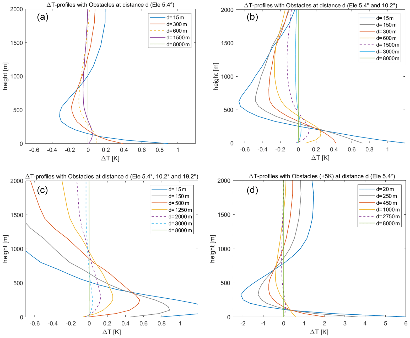
Figure 8 Impact of different obstacles on retrieved T profiles in a standard atmosphere. Depicted are the differences in T profiles with and without obstacles at give distances to the MWR. Panel (a) shows the impact of an ambient temperature obstacle at 5.4^∘ elevation, and panel (b) shows an obstacle which can be seen at 5.4 and 10.2^∘, while panel (c) shows an obstacle which can be seen at 5.4, 10.2, and 19.2^∘. Panel (d) shows the impact of a “heated” obstacle at different distances for 5.4^∘ elevation, which is 5 K warmer than its surroundings. Dashed lines indicate that the obstacle at this distance has an impact of ≤0.1 K on the T profile.

4.4 Identification of radio frequency interference (RFI)

Not only physical obstacles, pointing errors, or horizontal inhomogeneities but also RFI can have repercussions on MWR measurements (National Research Council, 2010). As an example, directional radio links and other telecommunication systems can be the source of such interferences, as their signal strength can be several orders of magnitudes stronger than normal atmospheric signals. In order to determine the strength and the direction of origin of interferences, full azimuth scans at several elevations are necessary. RFIs (as well as – to various degrees of accuracy – obstacles, instrument tilts and/or horizontal inhomogeneities) can be determined via the following proposed four-step method for every HATPRO with an azimuth motor (keep in mind that interval and threshold values are not fixed and can be adjusted as seen fit): (1) do full 360^∘ azimuth scans, e.g., with 10^∘ azimuth intervals at several elevations. (2) Check for clear-sky conditions. If the mean LWP of a 30 min interval before and after one scan is below 10 g m⁻² and its standard deviation below 4 g m⁻², then it is most likely clear-sky. (3) Calculate the difference of the T_B measurement of one azimuth angle and the minimum of a whole azimuth scan for each azimuth angle for each channel. This is also called the scan difference here. (4) If the scan difference is greater than a defined threshold, e.g., 1 K, a disturbance has been detected.

Figure 9 shows the percentage of cases in which the scan difference for the HATPRO at JOYCE is more than 1 K for the whole year of 2020 at 30^∘ elevation. High values in blue indicate significant disturbances. For K-band channels 1–7 at 60^∘ azimuth, we can clearly see a lightning rod, which has been installed near the HATPRO (less than 5 m away) in 2019. This disturbance always shows up within the K-band throughout 2020 to 2023 and is obviously a physical obstacle. The lightning rod is not detected in the V-band channels primarily due to the narrower beam width of the V-band receiver. This is mostly attributed to the combination of the 10^∘ azimuth step and the rod's slim profile, which results in the rod being predominantly positioned outside the field of view. Although it is possible that parts of the rod may be partially within the field of view, the limited coverage within the field of view is not substantial enough to have a noticeable impact on the measurements.

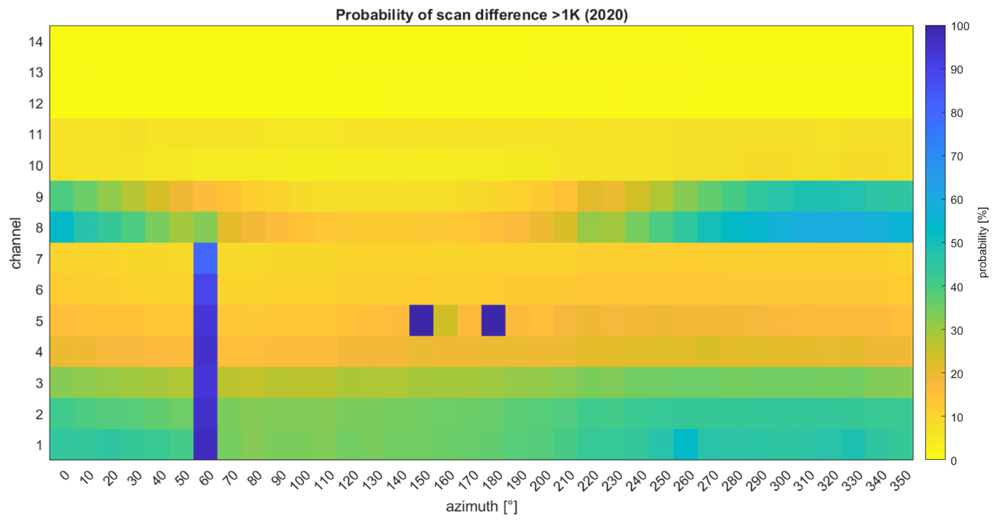
Figure 9 Mean probability of disturbance (the higher the percentage, the more pronounced the disturbance) from HATPRO azimuth scans at 30^∘ elevation for all 14 channels from 2020 at JOYCE. If the scan difference (T_B measurement at a certain azimuth angle minus the measured minimum T_B of a full 360^∘ azimuth scan) of a channel is greater than 1 K, a disturbance has been detected. Presented are only clear-sky conditions with a total of 7390 scans.

Another significant disturbance can be seen for channel 5 at 150 and 180^∘ azimuth. Channel 5 has a center frequency of 26.24 GHz, which is susceptible to frequencies used in communication links of which there are a few in and around the JOYCE site. That is why this disturbance is presumably due to RFI. As both of these significant disturbances are within the K-band, they pose no threat to T-profile retrievals. Even H-profile retrievals, which only use zenith pointing channels in the K-band, are not affected by these disturbances at 30^∘ elevation. However, they have to be taken into account and flagged when doing azimuth scans, which can be used for determining water vapor inhomogeneity.

Returning the focus to the V-band, channels 8 and 9, although used for T profiling, are also sensitive to humidity, as already discussed in Sect. 4.1. This can be seen in Fig. 9, too. Between 220 and 60^∘ azimuth, with a maximum at around 320^∘ in northwest, this behavior leads to a higher probability of disturbance and, therefore, to higher mean scan differences than in southeasterly directions during a whole year. These disturbances could theoretically be due to horizontal inhomogeneities in water vapor in the atmosphere, but, as already mentioned in Sect. 4.1, the mean impact of such conditions is low compared to the far greater impact a small tilt of the instrument can cause. That is why it is more probable that a small tilt to the northwest, and, therefore, a pointing error is the reason for these differences (compare with Sect. 4.2 and Fig. 4; therefore the tilt here has to be <0.3^∘). Note that the HATPRO which measured the RFI in Fig. 9 is not the same HATPRO as used in Sect. 4.1. As already discussed in Sect. 4.1, off-zenith disturbances in channels 8 and 9 have no impact on T profiling.

Nevertheless, even though all of the aforementioned disturbances do not affect T profiling (as they predominantly occur within the K-band or off-zenith within channels 8 and 9), they have to be monitored and assessed when installing an MWR at a new site, especially when azimuth scans are to be used to quantitatively analyze horizontal inhomogeneities of humidity.

5 Summary and conclusions

In this study, measurement uncertainties from HATPRO microwave radiometers and their impact on T profiling have been analyzed. These measurement uncertainties included horizontal inhomogeneities of the atmosphere, pointing errors or tilts of the instrument, physical obstacles which are in the line of sight of the MWR, and RFIs. On the one hand, the pointing errors and obstacles have been simulated with the help of a line-by-line RT model. The forward model implements radiosondes from RAO as input, and the T-profile retrievals utilize coefficients from RAO as well. On the other hand, the instrument misalignments, horizontal inhomogeneities, and an example of RFI have been analyzed through measurements on-site at JOYCE, and T-profile retrievals from those measurements utilize coefficients from nearby De Bilt, the Netherlands. Regarding the retrieval method, a statistical approach has been employed. The utilization of alternative retrieval methods, such as a physically based one, would not yield a different outcome for this study.

Mean north–south T_B differences at the same elevation angle during a 3-week period in summer 2022 can be mostly explained by a small tilt (about 0.3^∘) of the instrument and not by actual horizontal inhomogeneities. Therefore, before analyzing horizontal inhomogeneities, special care has to be taken to align the instrument perfectly horizontally. Within the V-band, the largest mean differences of T_Bs in north- and south-facing scans have been observed in channels 8–10 at 10.2 and 19.2^∘ elevation and are not exceeding 2.6 K, while for channels 11–14 they are always below 0.1 K. In order to achieve similar mean differences in T_Bs from actual horizontal inhomogeneities of water vapor from north- and south-facing scans in the V-band, an average ΔIWV≈3.4 kg m⁻² would be necessary, which is highly unlikely, and thus an instrument tilt is assumed. The impact of these measured mean north–south T_B differences on retrieved T profiles is small (median ΔT profile <0.08 K), as the channels 8–10, which show the largest mean differences and standard deviations at various elevations, are only used in zenith for T-profile retrievals. Actual horizontal inhomogeneities in the retrieved T profiles are represented in the percentiles range (25th and 75th percentile $\le \left|\mathrm{0.22}\mathrm{K}\right|$ beneath 3000 m).

Simulated pointing errors or tilts of the instrument up to ±1^∘ only show a small impact on T profiles. When using elevation scans in the T-profile retrievals, differences due to tilt do not exceed 0.1 K below 3000 m. When using zenith-only observations, tilts of up to ±1^∘ have almost no impact at all. In general, however, T-profile retrievals which make use of elevation scans are more precise and reliable than retrievals which do not, even when they have a tilt of 1^∘. The exact determination of the sources and magnitudes of tilts, whether originating from the setup (external misalignment, such as the instrument's placement on a table) or from the instrument itself (internal misalignment, such as a misaligned mirror within the HATPRO), remains a subject of ongoing investigation and may constitute a future research endeavor.

Physical obstacles like trees, masts, buildings, and mountains can have a strong impact on T_B measurements and T profiles, depending on their size, temperature, and distance to the radiometer location, especially at low elevations. Channels 8–10, which have the deepest penetration depths in the atmosphere, are most affected by simulated obstacles and can even “see” them from more than 10 km away at the lowest elevation angle of 5.4^∘, if they fill out the whole beam of the MWR in an inversion-free atmosphere. Channels 11–14 cannot reach as far into the atmosphere and can detect obstacles with ambient temperature at low elevations up to 3000–500 m away. When the temperatures of the obstacles are 5 K above their surroundings, these distances for channels 11–14 increase to around 5500–1600 m at low elevations. In order for an obstacle to have a minimal impact on T profiles of lower than 0.1 K, it has to be at least 600 m away. When the obstacle is 5 K warmer, this distance increases to at least 2700 m. Large obstacles like nearby mountains, which can also be seen in higher elevations, increase these distances further up to 4000 m in the worst case.

The impact of RFI on T profiling – at least in our example – is nonexistent, when they occur around or near commonly used frequencies for communication links, which are usually situated within the K-band (mostly between 20 and 30 GHz). These frequencies are not utilized in T-profile retrievals. However, RFI can negatively affect the analysis of observed T_Bs within the K-band in off-zenith directions, which bear the potential for deriving horizontal water vapor inhomogeneities.

In the following – with all these measurement uncertainties in mind – we will give some recommendations on how to properly set up a MWR. As a general rule, the operator needs to make sure that no obvious obstacles are near and around the scannable area of the MWR. If one locates possible obstacles, try to align the MWR in a way that there are no obvious obstacles in the preferred direction for elevation scans. While setting up the instrument, also make sure that the table on which the MWR is standing on is as level as possible, as even small tilts of under 0.5^∘ can still cause a rather big influence on T_B measurements in water vapor sensitive channels. After having done so (and after a recommended absolute calibration with liquid nitrogen) it is wise to initiate full azimuth scans at several elevations, similar to the four-step method described in Sect. 4.4, for as long as possible (a few days at clear-sky conditions would be optimal). This allows the operator to identify all sorts of disturbances in all the different compass directions and elevations for all frequency channels, from nearby obstacles and RFIs to probable tilts of the instrument (see Fig. 9 as an example). In practical scenarios, accurately estimating the temperature and appropriate distance of an obstacle can pose a challenge for the operator, particularly when the obstacle occupies only a small portion of the instrument's beam. This scanning method proves invaluable in such cases. If full azimuth scans are not feasible, at least elevation scans on both sides of the MWR are recommended, when there is the possibility to scan down to 5^∘ elevation in both directions. During regular operation, scanning in only one direction is sufficient though to retrieve accurate T profiles, when the instrument is set up properly. Directions with high disturbances should be avoided for obtaining retrieved products. In order to find out if a tilt arises from internal or external sources, one could set up an elevation scan at e.g., 30^∘ (north-facing) and 150^∘ (south-facing), so that the MWR will observe in the same direction. If T_B measurement from these two scans is different, then there might be a problem with the alignment inside the instrument.

Regarding on how strongly various T_B disturbances can affect measurements and profiling in more detail, more data in the form of simulations and measurements are needed. An interesting aspect for further analysis could be a more in-depth analysis of how exactly the emissivity, temperature, and size of an obstacle in the line of sight of the radiometer would influence measurements. Another interesting aspect would be a more detailed simulation of horizontal inhomogeneities of water vapor and also temperature and how they affect T profiling, especially in regard to pointing errors. With the help of mean azimuth scan differences, i.e. their amplitudes and phases, it is possible to determine the magnitude and direction of the instrument tilt. With that information it is theoretically possible to correct T_B measurements in hindsight. By conducting further simulated experiments under controlled conditions, it will be possible to assess the potential benefits of retrospective corrections and optimize correction algorithms. These future simulations hold promise for enhancing the accuracy and reliability of MWR measurements, ultimately contributing to improved atmospheric observations. Finally, there remains a lack of comprehensive understanding regarding RFIs and their implications on ground-based MWR measurements, necessitating further investigation (see also WMO statements and guidelines from the Expert Team on Radio Frequency Coordination⁷).