The transition to new ozone absorption cross sections for Dobson and Brewer total ozone measurements

Comparisons between total ozone column (TOC) measurements from ground-based Dobson and Brewer spectrophotometers and from various satellite instruments generally reveal seasonally varying differences of a few percent. A large part of these differences has been attributed to the operationally used Bass and Paur ozone cross sections and the lack of accounting for varying stratospheric temperatures in the standard total ozone retrieval for Dobson. This paper demonstrates how the use of new ozone absorption cross sections from the University of Bremen (Weber et al., 2016), as recommended by the Absorption Cross Sections of Ozone (ACSO) committee; the application of appropriate slit functions, especially for the Dobson instrument (Bernhard et al., 2005); and the use of climatological values for the effective ozone layer temperature (T_eff), e.g., from TEMIS (Tropospheric Emission Monitoring Internet Service), essentially eliminate these seasonally varying differences between Brewer and Dobson total ozone data (to generally less than ±0.5 %). For Hohenpeissenberg, the previous seasonal difference (close to 0 % in summer and up to 2.5 % in winter) is reduced to less than ±0.5 % year-round. Implementing this approach to the existing global network of Dobson spectrometers will reduce the overall uncertainty in their total ozone data from 3 % to 4 % previously to under 2 % at most locations.

1 Introduction

Ground-based total ozone column (TOC) measurements can be obtained by a large number of methods, but within the framework of the Global Atmosphere Watch program (GAW) of the World Meteorological Organization (WMO), Dobson and Brewer spectrophotometer measurements are considered to be reference observations. Worldwide, a large number of Dobson and Brewer instruments are used, and TOC measurements are routinely reported to the World Ozone and Ultraviolet Radiation Data Centre (WOUDC; https://woudc.org/, last access: 11 April 2024). Dobson spectrometers were developed in the 1920s and have been used for continuous measurements for decades (e.g., since 1926 in Switzerland; Stübi et al., 2021). Brewer spectrometers have been widely used since the 1980s. Both instruments have good long-term stability and precision (Stübi et al., 2017, 2021), and many research groups at different locations perform TOC measurements with the Brewer and Dobson instruments side by side. A seasonally varying systematic difference (or bias) between the two instruments has long been recognized (Kerr et al., 1988; Scarnato et al., 2010; Vanicek, 2006; Vaníček et al., 2012). Seasonally varying differences (biases) have also been found in the comparison of Dobson and Brewer total ozone data with data from satellite instruments (Koukouli et al., 2015, 2016).

Many of these differences have been attributed to the operationally used ozone absorption cross sections (Bass and Paur, 1985; Komhyr and Evans, 2008), which assume a fixed effective ozone temperature (−46.3 °C for the Dobson network; −45 °C for the Brewer network) and neglect the temperature sensitivity of these absorption cross sections (Koukouli et al., 2016; Köhler et al., 2018).

From 2008 to 2015, the Absorption Cross Section of Ozone (ACSO) committee evaluated a number of newly measured ozone absorption cross-section datasets and recommended using the data of Serdyuchenko et al. (2014) and Gorshelev et al. (2014) (henceforth denoted as SG14) for ground-based TOC measurements (Orphal et al., 2016). However, in the operational community, those recommendations are still not applied routinely.

Recently, Gröbner et al. (2021) and Redondas et al. (2014) retested different sets of ozone absorption cross sections and also accounted for their temperature dependence using ozone effective temperatures (T_eff) from modeled or measured data. In both studies, using the effective ozone temperature and the SG14 absorption cross section set reduced the difference between Brewer and Dobson total ozone data significantly to values below 1 %. For the comparison with various satellite instruments, Koukouli et al. (2016) also showed substantial improvements when applying a linear T_eff-dependent correction to the available Dobson data.

The purpose of this study is to check and further update the findings of Redondas et al. (2014), Orphal et al. (2016), and Gröbner et al. (2021). In addition, we address the following important points:

• We test the additional Weber et al. (2016) ozone absorption cross-section dataset, which is similar to Serdyuchenko et al. (2014) but has a better quantification of uncertainty and improved polynomial fitting coefficients for temperature dependence.

• We test two new ozone absorption cross-section datasets – Gorshelev et al., 2017, linked to Serdyuchenko et al., 2014, but with updated coefficients for temperature dependence, and Birk and Wagner (2021).

• We test different ways to account for the Dobson slit functions, which describe the instrument response to radiation at wavelengths near the nominal central wavelengths.

• We check ways to obtain ozone effective temperature and investigate their impact on TOC retrieval, including the comparison of daily effective temperature values with climatological values.

• We examine the effect of applying new temperature-dependent absorption cross-section datasets at different locations of Dobson and Brewer instruments worldwide.

• We provide recommendations on how to easily implement the new temperature-dependent ozone absorption coefficients in the operational Dobson TOC network.

The ultimate goal of this study is to pave the way for implementing the new temperature-dependent absorption cross sections in historical and operational retrievals for ground-based total ozone column (TOC) measurements.

2 Total ozone column measurements and retrieval

2.1 Measurement principle

Atmospheric concentration measurements by both instrument types are based on Beer–Lambert's law:

$$\begin{array}{}\text{(1)}& I\left(\mathit{\lambda }\right)=I_{\mathrm{0}}\left(\mathit{\lambda }\right){\exp }^{-\mathit{\tau }\left(\mathit{\lambda }\right)\mathit{\mu }},\end{array}$$

where I₀ and I are the wavelength-dependent solar irradiance at the top of the atmosphere and at the surface, respectively; τ is the optical depth of the atmosphere; and μ is the relative air mass (slant path through the atmosphere).

In the wavelength range between 300 and 345 nm, where both instruments measure TOC, ozone molecules are the main absorbers of solar irradiation. SO₂ absorption in this wavelength range can occur (Fioletov et al., 1998) but is typically small at most locations and can only be quantified by the Brewer instrument. Thus, the results shown in this study are limited to unpolluted air, where SO₂ values from Brewer instruments are low (< 1.0 Dobson units, DU).

Only taking into account the absorption of solar irradiance by the ozone molecules and correcting for Rayleigh scattering effects, Eq. (1) can be expressed as

$$\begin{array}{}\text{(2)}& I\left(\mathit{\lambda }\right)=I_{\mathrm{0}}\left(\mathit{\lambda }\right){\exp }^{-\left(\text{TOC}\mathit{\alpha }\right(\mathit{\lambda }){\mathit{\mu }}_{{\mathrm{O}}_{\mathrm{3}}}+\mathit{\beta }(\mathit{\lambda }\left)\frac{p_{\mathrm{S}}}{p_{\mathrm{0}}}{m}_{\mathrm{R}}\right)},\end{array}$$

where TOC is the vertical total column of ozone; ${\mathit{\mu }}_{{\mathrm{O}}_{\mathrm{3}}}$ is the relative air mass for ozone; α represents the wavelength-dependent ozone absorption coefficient; β is the wavelength-dependent Rayleigh extinction coefficient; p_S and p₀ are the atmospheric pressure at the station and at sea level, respectively; and m_R is the Rayleigh air mass.

Rearranging Eq. (2) gives

$$\begin{array}{}\text{(3)}& \text{TOC}\mathit{\alpha }\left(\mathit{\lambda }\right){\mathit{\mu }}_{{\mathrm{O}}_{\mathrm{3}}}=\ln \left(I_{\mathrm{0}}\right(\mathit{\lambda }\left)\right)-\ln \left(I\right(\mathit{\lambda }\left)\right)-\mathit{\beta }\left(\mathit{\lambda }\right){\displaystyle \frac{p_{\mathrm{S}}}{p_{\mathrm{0}}}}{m}_{\mathrm{R}}.\end{array}$$

This equation is valid for any wavelength. If measurements are taken at, e.g., two wavelengths, λ₁ and λ₂, one of the resulting two instances of Eq. (3) can be subtracted from the other, which gives

$$\begin{array}{}\text{(4)}& \begin{array}{rl}\text{TOC}\left(\mathit{\alpha }\right({\mathit{\lambda }}_{\mathrm{1}})-\mathit{\alpha }({\mathit{\lambda }}_{\mathrm{2}}\left)\right){\mathit{\mu }}_{{\mathrm{O}}_{\mathrm{3}}}=& \ln \left(I_{\mathrm{0}}\right({\mathit{\lambda }}_{\mathrm{1}}\left)\right)-\ln \left(I_{\mathrm{0}}\right({\mathit{\lambda }}_{\mathrm{2}}\left)\right)\\ & -\left(\ln \right(I\left({\mathit{\lambda }}_{\mathrm{1}}\right))-\ln (I\left({\mathit{\lambda }}_{\mathrm{2}}\right)\left)\right)\\ & -\left(\mathit{\beta }\right({\mathit{\lambda }}_{\mathrm{1}})-\mathit{\beta }({\mathit{\lambda }}_{\mathrm{2}}\left)\right){\displaystyle \frac{p_{\mathrm{S}}}{p_{\mathrm{0}}}}{m}_{\mathrm{R}}.\end{array}\end{array}$$

This approach can be expanded to more wavelengths and to any linear combination of the resulting equation, Eq. (3).

Consequently, TOC can be calculated from linear combinations of measurements at different wavelengths (λ_i):

$$\begin{array}{}\text{(5)}& \text{TOC}={\displaystyle \frac{\mathrm{\Delta }{F}_{\mathrm{0}}-\mathrm{\Delta }F-\mathrm{\Delta }\mathit{\beta }\frac{p_{\mathrm{S}}}{p_{\mathrm{0}}}{m}_{\mathrm{R}}}{\mathrm{\Delta }\mathit{\alpha }{\mathit{\mu }}_{{\mathrm{O}}_{\mathrm{3}}}}},\end{array}$$

where ΔF₀ and ΔF are the linear combinations of ln (I₀(λ_i)) and ln (I(λ_i)) and Δα and Δβ are the corresponding linear combinations of ozone absorption cross sections α(λ_i) and Rayleigh extinction cross sections β(λ_i). It is worth noting that in our study we applied the nominal Rayleigh scattering coefficients for both instruments from the standard algorithm (Bates, 1984; Komhyr and Evans, 2008) in contrast to, e.g., the study by Gröbner et al. (2021), who used a non-standard, updated Rayleigh scattering formulation.

$$\begin{array}{}\text{(6)}& {\displaystyle }\mathrm{\Delta }{F}_X={\sum }_{i=\mathrm{1}}^n{w}_i\ln \left(I_X\right({\mathit{\lambda }}_i\left)\right)\text{(7)}& {\displaystyle }\mathrm{\Delta }\mathit{\beta }={\sum }_{i=\mathrm{1}}^n{w}_i{\mathit{\beta }}_i\text{(8)}& {\displaystyle }\mathrm{\Delta }\mathit{\alpha }={\sum }_{i=\mathrm{1}}^n{w}_i{\mathit{\alpha }}_i\end{array}$$

Potential aerosol influences are minimized using multiple wavelengths – e.g., four single-slit measurements with appropriate weights in the case of the Brewer instrument (Redondas et al., 2014) or two-wavelength pairs in the case of the Dobson instrument (typically AD or CD, where the A pair uses wavelengths near 305 and 325 nm, the C pair wavelengths near 311 and 332 nm, and the D pair near 317 and 340 nm; see also Komhyr and Evans, 2008). The coefficients w_i of the linear combinations for the sums in Eqs. (6)–(8) for both Dobson and Brewer instruments are given in the last columns of Tables 1 and 2. Note that these weights fulfill the equations $\sum w_i{\mathit{\lambda }}_i^{\mathrm{0}}=\mathrm{0}$ and $\sum w_i{\mathit{\lambda }}_i^{-\mathrm{1}}\approx \mathrm{0}$. This means that extinctions by processes with a wavelength dependence of λ⁰ or λ⁻¹, i.e., typical cloud or aerosol scattering, cancel each other out and would not affect the retrieved total ozone columns (see also Redondas et al., 2018; note the missing exponent −1 in their Eq. 6).

Table 1 Central wavelength (mean; nm), full width at half maximum (FWHM; nm), and base (nm) and top (nm) for the Bernhard slit approximation for the individual slit functions of Dobson104. The nominal values were obtained from the Dobson operations handbook (Komhyr and Evans, 2008). The Bernhard values were obtained from Table 1 in Bernhard et al. (2005). It is important to note that a corrected value (2.12 nm) for the top of A2 was applied. The weights w_i (in the last column) are required to calculate the final absorption coefficients Δα as described in Sect. 2.1 and 2.6 and Eq. (8).

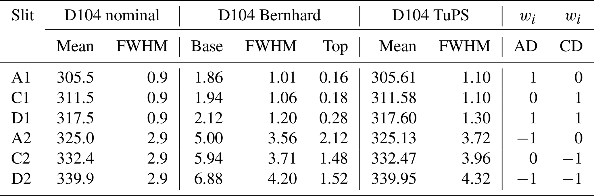
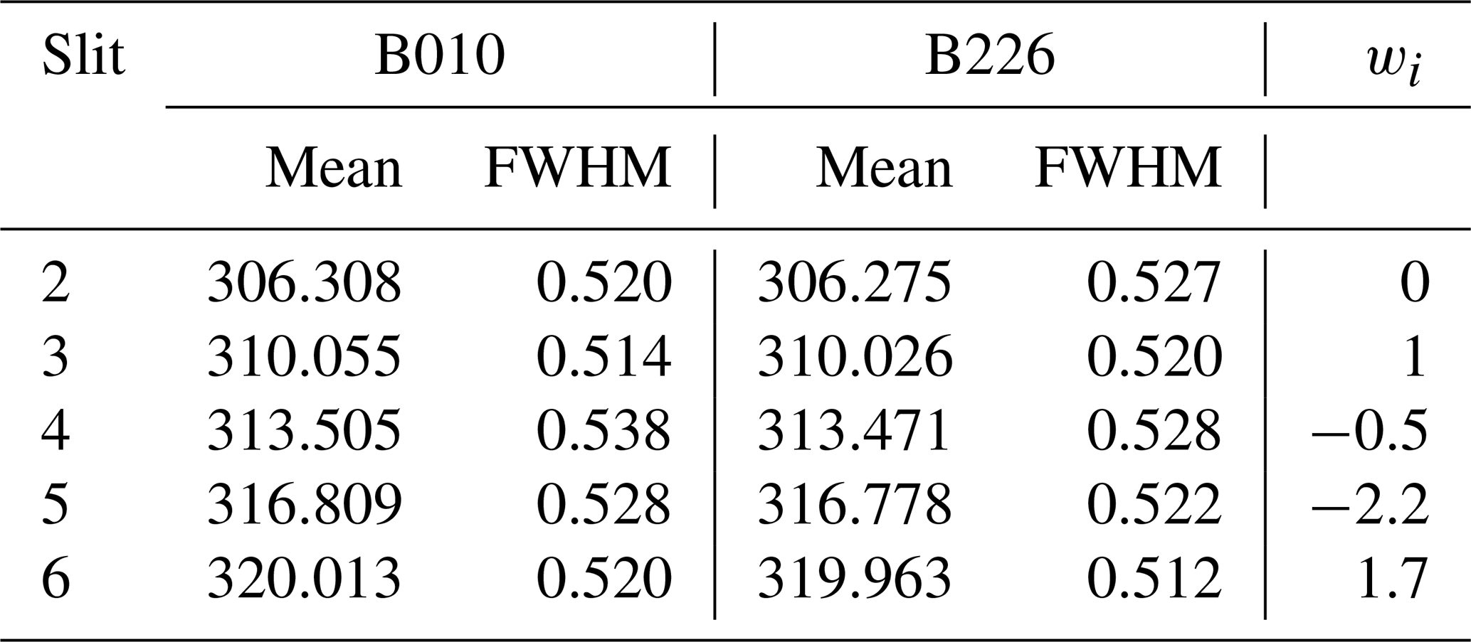
Table 2 Central wavelength (mean; nm) and full width at half maximum (FWHM; nm) of the individual slit functions for the Brewer instruments. The weights w_i (in the last column) are required to calculate the final absorption coefficients Δα as described in Sect. 2.1 and Eq. (8).

2.2 Brewer and Dobson spectrophotometers measurements at Hohenpeissenberg

The Brewer spectrometer is fully automated. In ozone mode it measures solar irradiance at six nominal wavelengths in the UV range, from 303.2 to 320.1 nm, quasi-simultaneously. This is achieved using a slit mask in combination with holographic grating and a photomultiplier tube. The calculation of TOC following Eq. (5) uses measurements only at the four longest wavelengths of the six. A detailed description of the Brewer instrument can be found in Brewer (1973), Kerr et al. (1985), and Redondas et al. (2018).

Two Brewer instruments are currently in operation at the Hohenpeissenberg Meteorological Observatory. Brewer010 is a single-monochromator Brewer MKII that has continuously measured TOC since 1983. The MKIII double-monochromator Brewer226 has been continuously measuring TOC since 2015. Both instruments are calibrated once a year by comparing them with the reference travelling standard single-monochromator Brewer017, operated by the International Ozone Services (IOS).

The Dobson spectrometer measures TOC by comparing the relative intensities at two of the three wavelength pairs in the UV wavelength range from 305.5 to 339.9 nm. These wavelength pairs are referred to as A, C, or D (the B pair is normally not used). Each pair compares solar irradiation in a “short” wavelength band that is highly absorbed by ozone to solar irradiation in a “long” wavelength band that is less affected by ozone. For each measurement, an optical attenuator (a.k.a. “wedge”) is gradually adjusted to reduce the higher light intensity at the long wavelength until it is equal to the lower light intensity at the short wavelength. With the information on the exact ratio between the long- and short-wavelength intensities, TOC values are then determined using the double ratio of two pair measurements following Eq. (5). Typically, the A and D pairs are the most widely used pairs.

Hohenpeissenberg has been using Dobson104 operationally since 1968, with emphasis on direct sun AD measurements. For this study, we exclusively use AD measurements. Typically, these measurements are performed only from Monday to Friday, resulting in approximately 1200 measurements per year. Dobson104 undergoes regular calibration by comparison with the Dobson reference instrument Dobson064, maintained by the Regional Dobson Calibration Center Europe and also located at Hohenpeissenberg. The most recent calibration of Dobson104 was in 2019.

Internal stray light can affect both Brewer and Dobson instruments, as noted by Karppinen et al. (2015), Moeini et al. (2019), and Scarnato et al. (2009). Typically, the impact of stray light manifests as lower TOC values at high ozone slant path values. This means that, at low sun elevation angles and high TOC values, the TOC retrieved by these instruments is underestimated, as indicated by Bais et al. (1996) and Redondas et al. (2014). However, double-monochromator Brewers are much better equipped to suppress stray light, resulting in minimal stray light effects.

As mentioned, both types of instruments are reference measurement systems for ground-based TOC measurements in the GAW program. Thus, they should yield similar TOC values when measuring side by side. For comparison between the two instrument types in this study, the following data processing filters were applied:

• The time period between Dobson and Brewer measurements was ≤15 min.

• Multiple Dobson measurements within a time interval of ≤15 min were averaged.

• Ozone air mass was ≤3.6.

• SO₂ from Brewer was ≤1.0 DU.

• The time period was May 2008–December 2021 for the comparison between Dobson104 and Brewer010.

• The time period was June 2018–December 2021 for the comparison between Dobson104 and Brewer226.

In total, we used 8135 measurements to compare Dobson104 with Brewer010, around 1300 of those taken during the winter season and 2300 taken during summer. For the comparison of Brewer226 with Dobson104, we used 2250 measurements, around 420 of those taken during winter and 760 taken during summer.

Figure 1 shows the typical distinct seasonal cycle in the difference in TOC values from Brewer and Dobson instruments. Throughout the summer months, both instruments give very similar total ozone columns. During the winter months notable differences arise, and the Dobson instrument typically reports 1 % to 2 % smaller TOC values than Brewer010 (up to 3 % for Brewer226; see Supplement). In the annual average, this results in a difference of about 1 % between Brewer010 and Dobson104 TOC and about 1.4 % between Brewer226 and Dobson104. Very similar differences are reported for other locations and instruments (e.g., Gröbner et al., 2021; Redondas et al., 2014).

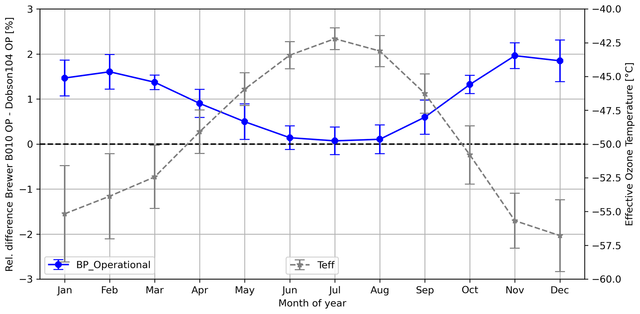
Figure 1 Average monthly-mean (1990–2020) differences between Brewer010 and Dobson104 (blue line) calculated using the operationally used standard Bass and Paur ozone absorption cross sections. The dashed grey line gives the average monthly means of effective ozone temperature (T_eff) based on measurements at Hohenpeissenberg (see Sect. 2.5 for details). The error bars represent the standard deviation (1σ; 1990–2020).

2.3 Slit functions

Since both Dobson and Brewer instruments measure with limited spectral resolution, it is necessary to consider the spectral variation in the ozone cross section over the wavelength bands covered by the instrument. Typically, the varying sensitivity in each wavelength band is called the slit function. The high-resolution ozone cross section needs to be convolved over these slit functions, yielding an effective ozone cross section for each measured wavelength or wavelength pair.

2.3.1 Dobson

The Dobson network uses two slightly different parametrizations for the typical slit functions. Both parametrizations are based on the measured slits of Dobson083 (Komhyr et al., 1993), the primary standard in the world, which are quite similar to recently measured slit functions of Dobsons using tuneable lasers (Köhler et al., 2018). The Dobson operations handbook (Komhyr and Evans, 2008) assumes a triangular slit function for the three short-wavelength slits. Bernhard et al. (2005) assume trapezoids for the same short-wavelength bands (Fig. 2). The long-wavelength slits are parametrized as trapezoids in both approximations. In addition to these standard parametrizations, slit functions have also been measured directly using a tuneable and portable radiation source (TuPS), developed in the European Metrology Research Programme (EMRP) joint research project ENV59, ATMOZ (Šmíd et al., 2021). The slits of the Dobson104 were measured with a TuPS in October 2017, and the resulting slit functions were also tested here. They are shown in Fig. 2 (red lines). For the short-wavelength slits in particular (e.g., slit A1 in Fig. 2a), it is important to consider the relatively wide wings of the TuPS slit function (dotted red line in Fig. 2a). Also at the short wavelengths, below 304 nm in Fig. 2a, the large ozone cross sections make a considerable contribution to the effective ozone cross section, which is integrated over the entire slit function (see also Gröbner et al., 2021).

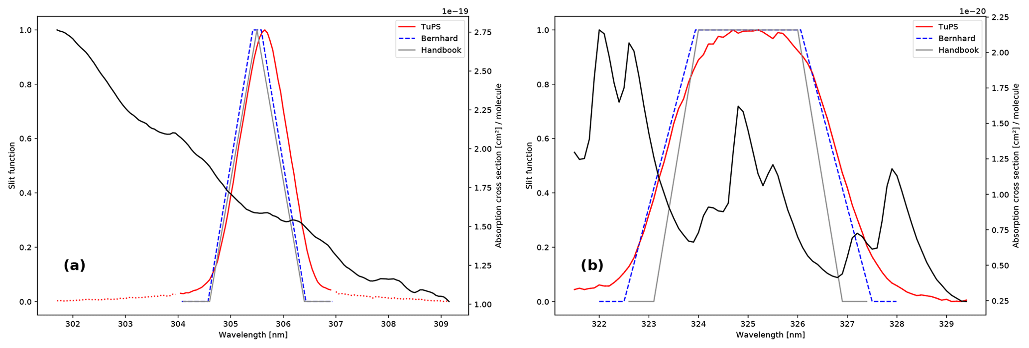
Figure 2 Parametrized and measured slit functions. Grey line: Dobson operations handbook. Blue line: Bernhard et al. (2005). Red line: measured slit functions (TuPS) for the Dobson104. TuPS measurements of Dobson104 were combined with TuPS measurements from Dobson101 (dotted red line; only for slits A1 and D1) to extend the spectral range of the slit function. It is important to note that a corrected value (2.12 nm) for the top of the long wavelength of the A pair was applied. Panel (a) represents the short wavelengths, and panel (b) represents the long wavelengths of the A wavelength pair. The black line gives the SG16 (Weber et al., 2016) absorption cross section at a temperature of −55 °C.

The slit parameters (central wavelength, FWHM of each slit, and base and top for Bernhard slit approximation) for Dobson104 are shown in Table 1.

2.3.2 Brewer

Slit functions for each Brewer instrument are derived from dispersion tests, which are typically part of the yearly calibration. A detailed explanation of the calibration process and the computation of the dispersion relation are given in Gröbner et al. (1998) and Redondas et al. (2018). In short, the scanning mode, in combination with the emission lines of different discharge lamps, is used to determine the central wavelength and the FWHM of every slit by analyzing the measured photon counts as a consequence of the illumination. In the standard operating procedure, the resulting triangle function of each slit is then truncated at 0.87 of the maximum height and thus parametrized as a trapezoid. The results of the calibration process are typically given in a file (lf-file) and are summarized in Table 2 for both Brewer instruments. Brewer slit functions are instrument-specific and can also vary over time. Redondas et al. (2018), using Brewer slit functions measured by a tuneable laser system similar to Köhler et al. (2018), report changes in the effective ozone absorption coefficients on the order of 0.8 %. This is similar to the magnitude of changes we find for different Dobson slit measurements or parametrizations (Köhler et al., 2018).

2.4 Ozone absorption cross sections

The operational TOC retrieval for Brewer and Dobson instruments relies on the ozone absorption cross section measured by Bass and Paur (1985; henceforth B&P). As mentioned, several studies (Fragkos et al., 2015; Gröbner et al., 2021; Orphal et al., 2016; Redondas et al., 2014) suggest using updated ozone absorption cross sections. This study focuses on four sets of ozone absorption cross sections, all of which cover the wavelength range from 300 nm to 345 nm for the Brewer and Dobson spectrometers. Additionally, only datasets providing a quadratic polynomial approximation for the T_eff dependency of the cross sections were considered.

• SG14. This dataset (Gorshelev et al., 2014; Serdyuchenko et al., 2014) comes from the Institute of Environmental Physics at the University of Bremen. It provides data in the spectral range of 213–1100 nm with a spectral resolution of 0.02–0.24 nm. Temperature sensitivity was measured at 10 K intervals between 193 and 293 K. Here, we use the dataset downloaded from https://www.iup.uni-bremen.de/gruppen/molspec/databases/referencespectra/o3spectra2011/index.html (last access: 11 April 2024). According to the authors, the dataset's uncertainty is 2 % to 3 % depending on the wavelength range. This is consistent with other cross-section measurements. Recent studies (Gröbner et al., 2021; Orphal et al., 2016; Redondas et al., 2014) have recommended this dataset which minimizes the discrepancy between Dobson and Brewer measurements. Note that these studies referred to the dataset as IUP or SER.

• SG16. This dataset (Weber et al., 2016) is very similar to the SG14 dataset, but it additionally provides detailed wavelength-dependent uncertainty information based on Monte Carlo simulations and including uncertainties from the temperature parametrization, as well as uncertainties from the laboratory measurements. The dataset was obtained from https://www.iup.uni-bremen.de/UVSAT/data/xsectionuncertainty/ (last access: 11 April 2024). The authors estimated an uncertainty of 1.1 % to 3 % depending on wavelength. In the Huggins band, for example, the overall uncertainty was estimated to be 1.5 % (1σ).

• G17. This dataset (Gorshelev et al., 2017) is also linked to the abovementioned datasets. It was created as part of the ATMOZ (“Traceability for Atmospheric Total Column Ozone”) joint research program (JRP) funded by the EMRP. It covers the wavelength range of 295–350 nm and is available for 11 temperatures between 193 and 293 K. The polynomial quadratic equation is not publicly available but was provided via personal communication (Mark Weber, personal communication, 2023). Currently, no peer-reviewed publication with comprehensive details is available. However, the authors mention (Gorshelev et al., 2017) that the combined uncertainties are below 1 % and only increase near the spectral boundaries of the measurements. This dataset is similar to the dataset referred to as IUP_A in Gröbner et al. (2021), albeit with updated polynomial coefficients for the temperature dependency.

• BW. The dataset (Bak et al., 2020; Birk and Wagner, 2021) was measured within the framework of the ESA project SEOM-IAS at the German Aerospace Center for the wavelength range 243–346 nm and at six temperatures in the range of 193–293 K. Their polynomial temperature parametrization was downloaded from the Zenodo repository https://zenodo.org/record/4423918#.ZCFXQfbP1aT (last access: 11 April 2024). Notably, we use version 2 of the dataset from the Zenodo repository. Currently, no peer-reviewed publication containing all details is available. This dataset is similar to the dataset referred to as ACS in Gröbner et al. (2021), who, however, determined their own polynomial temperature dependence.

Generally, the temperature dependence of all four new ozone cross sections uses a quadratic polynomial (see also Bass and Paur, 1985; Weber et al., 2016):

$$\begin{array}{}\text{(9)}& {\mathit{\sigma }}_T=C_{\mathrm{0}}+C_{\mathrm{1}}T+C_{\mathrm{2}}{T}^{\mathrm{2}},\end{array}$$

where C₀, C₁, and C₂ are the temperature coefficients (provided in the datasets). Figure 3 illustrates the influence of various temperatures on the ozone absorption cross sections for the SG16 dataset (blue lines). Differences between the B&P and SG16 cross sections are shown by the dashed red line. Below 320 nm, these differences are quite small. Above 325 nm, however, they become larger and often exceed several percent. Similarly, from the differences between the various blue lines, one can see that temperature effects are generally much larger at wavelengths longer than about 330 nm.

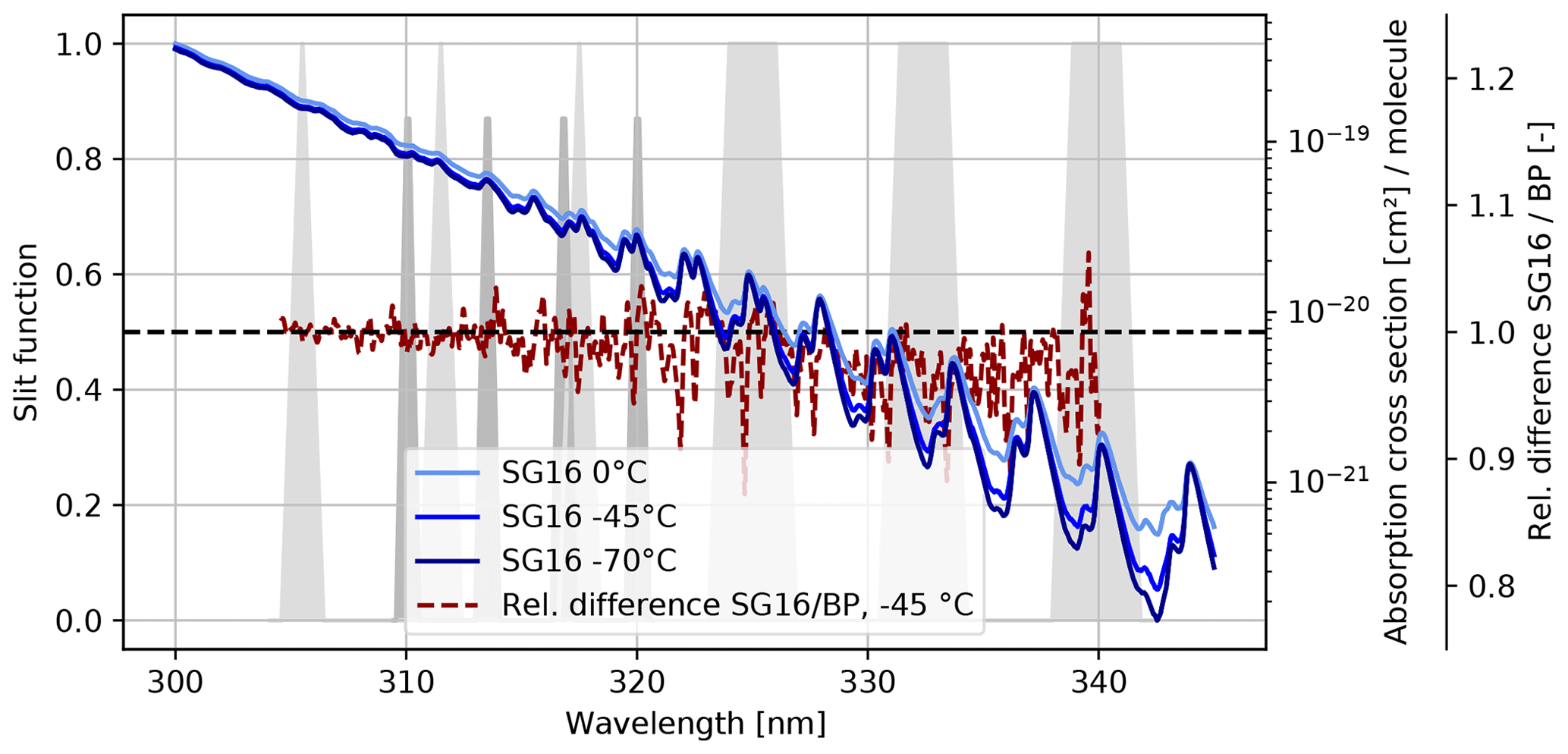
Figure 3 Ozone absorption cross sections based on the SG16 dataset for three selected temperatures (blue curves). The red line shows the relative difference between the SG16 and B&P datasets for a temperature of −45 °C. The Dobson (light grey) and Brewer (dark grey) slit functions are shown as well.

Examining the differences between cross sections at the location of the slit functions illustrated in Fig. 3 for Brewer (dark grey; below 320 nm) and Dobson (light grey; extending above 320 nm), it becomes evident that the transition from B&P to SG16 cross sections along with the introduction of temperature-dependent ozone cross sections will have a much larger effect on the Dobson data, whereas its impact on the Brewer data should be relatively minor.

It is also worth noting that the vacuum wavelengths have to be converted to wavelengths in the air. To do so, we utilized a Python script from GitHub (https://github.com/polyanskiy/refractiveindex.info-scripts/blob/master/scripts/Ciddor%201996%20-%20air.py, last access: 11 April 2024), which employs the equation proposed by Ciddor (1996). Standard values for the input parameter (e.g., CO₂ concentration of 400 ppm, air pressure of 1013.25 hPa, relative humidity of 50 %, and temperature of 15 °C) can be consistently applied throughout the year without significantly compromising the quality of the conversion.

2.5 Effective ozone temperature

We follow other studies (Gröbner et al., 2021; Redondas et al., 2014; Scarnato et al., 2009; Vanicek, 2006) and use the effective ozone temperature T_eff to describe the temperature effect of the ozone absorption cross sections. T_eff can be computed from the vertical profiles of temperature T(z) and ozone density O₃(z) based on the following equation:

$$\begin{array}{}\text{(10)}& T_{\text{eff}}={\displaystyle \frac{\int T\left(z\right){\mathrm{O}}_{\mathrm{3}}\left(z\right)\mathrm{d}z}{\int {\mathrm{O}}_{\mathrm{3}}\left(z\right)\mathrm{d}z}}.\end{array}$$

Generally, T_eff can be derived from modeled data or from measurements. In our case, we compared two different T_eff datasets to check whether the two approaches have significant differences:

• The TEMIS (Tropospheric Emission Monitoring Internet Service) dataset contains T_eff values based on data from the European Centre for Medium-Range Weather Forecasts (ECMWF). T_eff data prior to 2000 rely on ERA-40, while data from 2000 onwards are based on the operational ECMWF analysis (Ronald van der A, personal communication, 2024). Further information on the dataset can also be found in Van der A et al. (2010). We downloaded station overpass files for Hohenpeissenberg and other locations from the TEMIS website at https://www.temis.nl/climate/efftemp/overpass.php (last access: 11 April 2024).

• The OS_LIDAR dataset combines ozonesonde measurements (altitude < 29 km) with lidar measurements (altitude ≥ 29 km) from Hohenpeissenberg.

Missing lidar or ozonesonde observations were filled using linear interpolation between available measurements. To ensure correct T_eff calculations, it is necessary to use vertical profiles of T and O₃ from the ground up to about 50 km altitude, where the O₃ density approaches zero. For the case of Hohenpeissenberg, using only ozonesonde data, which only reach burst heights of approximately 30–35 km, would result in a low bias of about 2.2 °C (dotted green lines in Fig. 4).

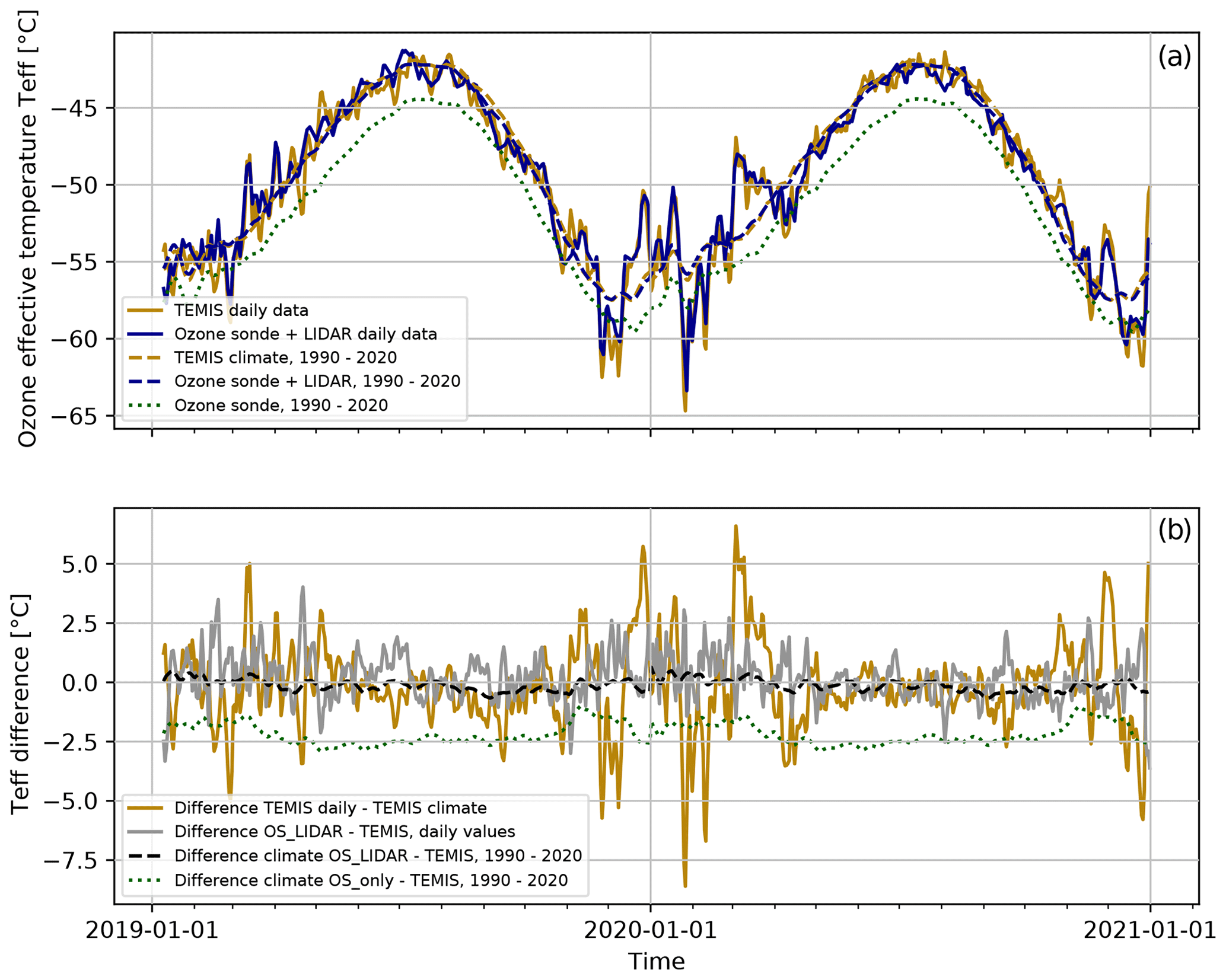
Figure 4 Time series of ozone effective temperature T_eff at Hohenpeissenberg based on TEMIS, on ozonesonde data (OS_only), or on combined ozonesonde (OS) and lidar data (a). The climatological values (climate; dashed orange lines) are calculated from daily values over the time period 1990–2020. Additionally, a 7 d rolling mean is applied. Panel (b) shows the daily difference between the TEMIS- and OS/OS_LIDAR-derived datasets.

Figure 4 depicts the temporal evolution of T_eff over a 2-year period along with the 30-year T_eff climatology (1990–2020) for both datasets (TEMIS and OS_LIDAR) at the Hohenpeissenberg site. The figure demonstrates the small differences between the two datasets and the sometimes larger differences between daily and climatological values. While the climatological difference between TEMIS and OS_LIDAR is almost negligible, there can be differences of up to ±2.5 °C between daily T_eff data from the two sources (grey line in the bottom panel of Fig. 4). However, in general, the two datasets are very similar, with a mean difference of approximately 0.1 °C and a standard deviation of about 1.2 °C for daily values in the 1990–2020 time frame.

Larger differences occur between daily and climatological values (orange line in the bottom panel of Fig. 4). Especially in winter, the difference between daily and climatological values can reach ±8 K. Overall, the differences are lower than a few kelvins and have a standard deviation of 2.2 °C for the TEMIS dataset. This is comparable to the scale of differences between the TEMIS and OS_LIDAR datasets.

In summary, Fig. 4 indicates that the use of climatological values for T_eff already provides a very good representation of temperature variations over the year. In summer, very little can be gained from using daily values. Even in winter, the differences between daily and climatological values are of similar magnitude to the differences between the TEMIS and OS_LIDAR datasets. These findings bear significant relevance for selecting an appropriate dataset for operational or reprocessing purposes.

A look at the seasonal variation in T_eff in other locations worldwide is presented in Fig. 5. Generally, stations at higher latitudes have a higher amplitude of the seasonal T_eff cycle. In addition, higher latitudes also see much higher variability in T_eff, especially during winter and spring, as clearly shown by the shaded regions in Fig. 5.

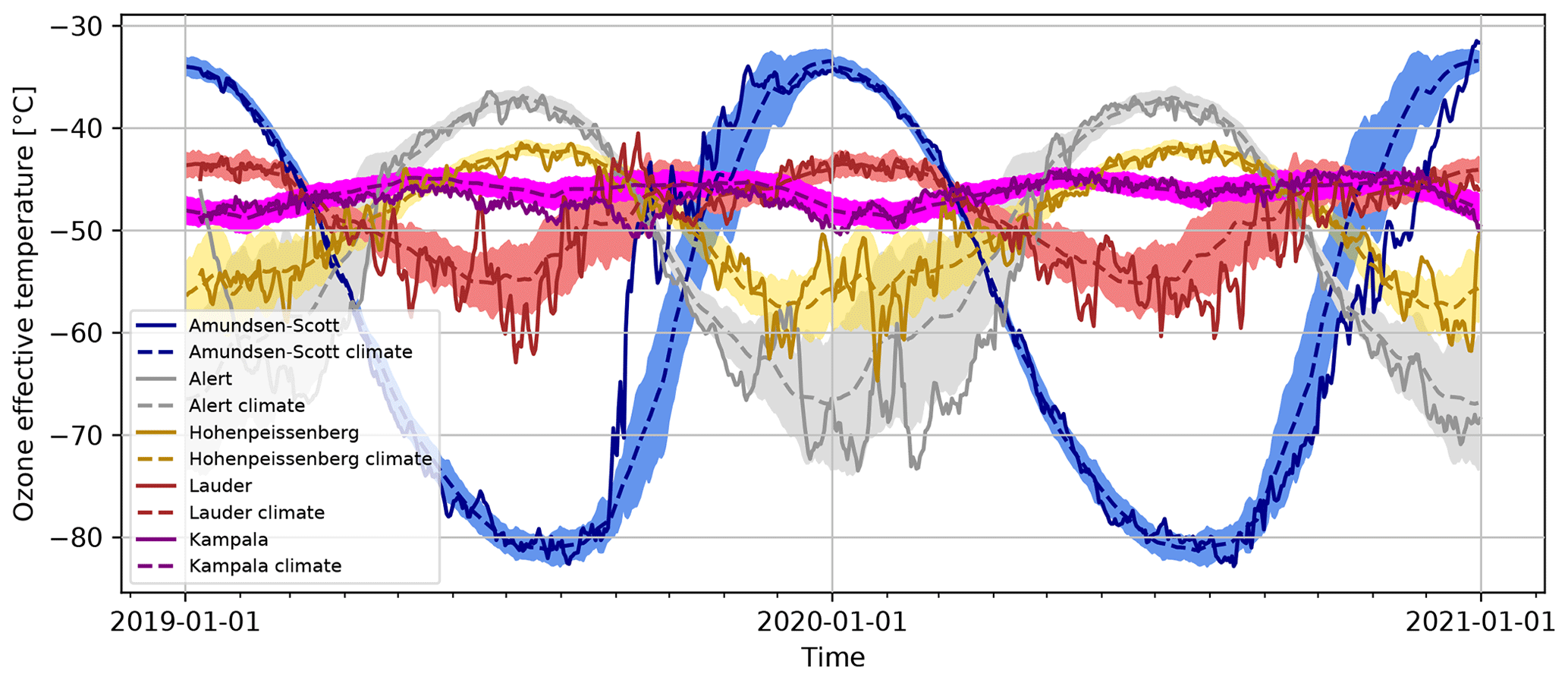
Figure 5 Time series of TEMIS-derived ozone effective temperature T_eff for five locations covering latitudes from −90° (Amundsen–Scott) to +82.5° (Alert). Hohenpeissenberg is at 48° N, Kampala at 0°, and Lauder at 45° S. The dashed lines indicate the long-term climatology (1990–2020), and the shaded areas indicate the year-to-year variability (1σ).

2.6 Ozone absorption coefficients

We use the standard approach based on Komhyr et al. (1993) to calculate the differential ozone absorption coefficients Δα for Brewer and Dobson instruments. The approach involves using the effective ozone temperature T_eff, the polynomial temperature approximation for the ozone absorption cross sections σ(λ,T_eff), and the slit functions S_i(λ) for slit i to calculate α_i. This approach is used and discussed in detail in multiple studies (Bernhard et al., 2005; Gröbner et al., 2021; Redondas et al., 2014, 2018). It is defined by the following equation:

$$\begin{array}{}\text{(11)}& {\mathit{\alpha }}_i={\displaystyle \frac{\int \mathit{\sigma }(\mathit{\lambda },T_{\text{eff}})S_i\left(\mathit{\lambda }\right)\mathrm{d}\mathit{\lambda }}{\int S_i\left(\mathit{\lambda }\right)\mathrm{d}\mathit{\lambda }}}.\end{array}$$

Applying the polynomial expression for the ozone cross sections (Eq. 9) and rearranging the equation provides a polynomial equation for α_i using T_eff and a set of coefficients A_ij:

$$\begin{array}{}\text{(12)}& {\mathit{\alpha }}_i\left(T_{\text{eff}}\right)=A_{i\mathrm{0}}+A_{i\mathrm{1}}\cdot T_{\text{eff}}+A_{i\mathrm{2}}\cdot T_{\text{eff}}^{\mathrm{2}},\end{array}$$

with

$$\begin{array}{}\text{(13)}& A_{ij}={\displaystyle \frac{\int C_j\left(\mathit{\lambda }\right)S_i\left(\mathit{\lambda }\right)\mathrm{d}\mathit{\lambda }}{\int S_i\left(\mathit{\lambda }\right)\mathrm{d}\mathit{\lambda }}},\end{array}$$

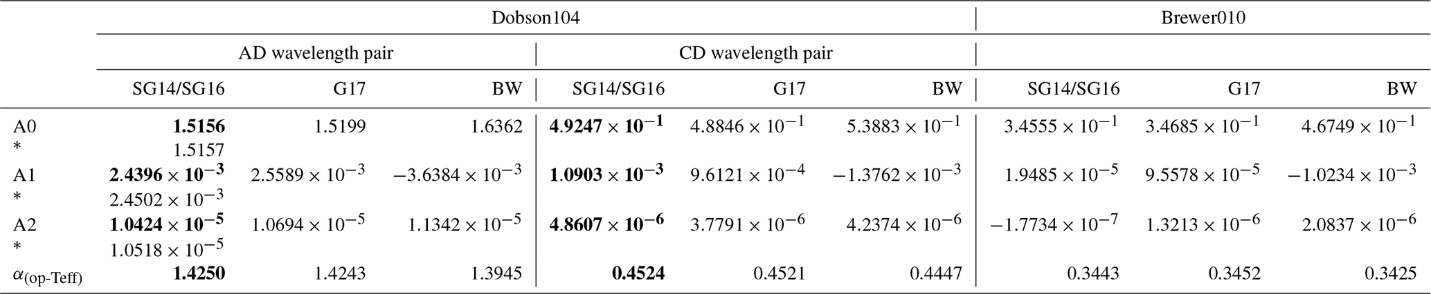
where C_j(λ) represents the coefficients for temperature dependence from Eq. (9) and S_i(λ) represents the slit functions. The resulting A_ij coefficients for individual slits of the Dobson instrument based on the SG16 ozone absorption cross-section dataset are listed in Table 3. The combined coefficients required for a Brewer or Dobson TOC measurement (see Eq. 5) – e.g., for the AD wavelength pair (AD = A–D) – are obtained by summing up the individual, slit-dependent coefficients, with their corresponding weights following Eq. (8).

Note that the coefficients in Table 3 are very similar to those published by Redondas et al. (2014), which, to our knowledge, is the only reviewed publication that directly reported the coefficients utilizing the new ozone cross sections.

Table 3 Coefficients for the temperature dependence (in °C) of the effective ozone absorption cross section for the different Dobson slits (A, C, and D). Results are based on the SG16/SG14 dataset and the slit approximation from Bernhard et al. (2005). For values of the ozone absorption coefficient at the currently fixed T_eff, see Table 5. Numbers in bold show the suggested new coefficients for total ozone column (TOC) computations utilizing the AD and CD wavelength pairs.

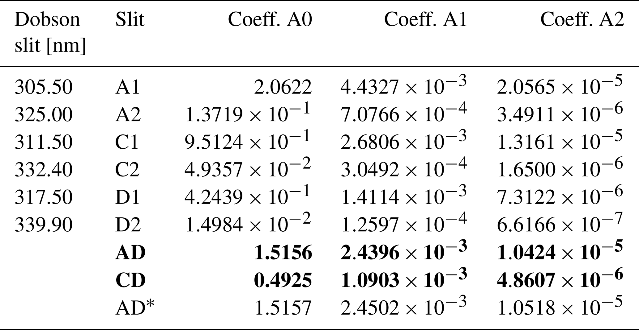
^∗ Data from Redondas et al. (2014).

Table 4 summarizes the resulting coefficients for the temperature dependence of the combined differential ozone absorption coefficients. Results are shown for different ozone cross-section datasets and for Dobson104 and Brewer010. Due to their potentially different instrument-specific slit functions, other Brewers have slightly different coefficients. Based on the mean of 123 dispersion tests of 33 Brewer instruments, Redondas et al. (2014), for example, calculated coefficients using the SG14 dataset ($\text{A0}=\mathrm{3.4591}\times {\mathrm{10}}^{-\mathrm{1}}$; $\text{A1}=\mathrm{2.8781}\times {\mathrm{10}}^{-\mathrm{5}}$; $\text{A2}=-\mathrm{4.9188}\times {\mathrm{10}}^{-\mathrm{8}}$); the results were comparable to ours and gave an instrument-specific Δα within 0.06 % of our Brewer010 value. Note also the much smaller temperature dependence for the Brewer where A1 and A2 are about 2 orders of magnitude smaller than for the Dobson.

Table 4 Coefficients for the temperature dependence of the combined ozone absorption coefficient for the main Dobson wavelength pairs (AD and CD) and for the Brewer010. For the Dobson instrument, the slit approximation from Bernhard et al. (2005) was applied. Results are shown for the different ozone cross-section datasets. SG14 and SG16 are combined because results are very similar. Numbers in bold show the suggested new coefficients for total ozone column (TOC) computations utilizing the AD and CD wavelength pairs.

^∗ Data from Redondas et al. (2014).

Finally, Table 5 gives a comparison of the effective differential ozone absorption coefficients at the fixed temperatures currently used for Dobson and Brewer instruments (i.e. for the different cross-section datasets and different slit functions). For the Dobson, all new cross-section datasets give 0.5 % to 3.3 % smaller effective ozone absorption coefficients than B&P. This would result in correspondingly larger total ozone values. BW stands out with the smallest effective absorption coefficient. These results are very similar to Gröbner et al. (2021) and Redondas et al. (2014), which are also shown in the table. Note, however, the slightly smaller effective cross sections (about 0.7 % smaller) for the handbook's slit functions for Dobson104 compared to Bernhard or the TuPS.

Table 5 Effective differential ozone absorption coefficient (in atm cm⁻¹) at the nominal fixed T_eff for the different ozone cross-section datasets for Dobson and Brewer instruments. The Dobson results are given for three different slit functions. The fixed operational T_eff is −46.3 °C for Dobsons and −45 °C for Brewers. Numbers in bold show the suggested new coefficients for total ozone column (TOC) computations utilizing the AD and CD wavelength pairs.

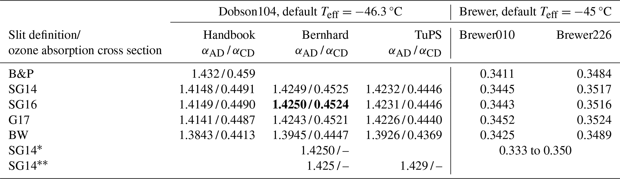
^∗ Data from Redondas et al. (2014) for Brewer based on 33 instruments and 123 dispersion tests. ${}^{\ast \ast }$ Data from Gröbner et al. (2021).

For the Brewers, all new cross-section datasets give 0.1 % to 1.2 % larger effective ozone absorption coefficients than B&P. This would result in correspondingly smaller total ozone values. Here, all cross sections result in similar values of Δα. As mentioned, the Brewers have different slit functions for different instruments. Here, this results in about 2 % larger Δα for Brewer226 compared to Brewer010. Both are within the range of Δα reported by Redondas et al. (2014). Based on 33 Brewer instruments and 123 dispersion tests, they report values between 0.335 and 0.350 cm⁻¹ for both the B&P and the SG14 datasets.

When the new effective differential ozone cross sections are known, the relationship between TOC and Δα in Eq. (14) allows for easy reprocessing of TOC values. Currently, the differential ozone absorption coefficient Δα_OP is based on the B&P cross sections at a fixed temperature and the Komhyr parametrization. By applying the following equation, the corresponding old operational TOC values can easily be recalculated to the new ozone cross sections $\mathrm{\Delta }{\mathit{\alpha }}_{T_{\text{eff}}}$ with varying T_eff:

$$\begin{array}{}\text{(14)}& {\text{TOC}}_{T_{\text{eff}}}={\text{TOC}}_{\text{OP}}{\displaystyle \frac{\mathrm{\Delta }{\mathit{\alpha }}_{\text{OP}}}{\mathrm{\Delta }{\mathit{\alpha }}_{T_{\text{eff}}}}}.\end{array}$$

As mentioned, knowledge about the slit functions is necessary. This is easier for the Dobson instrument, as the slit functions are wider and generally quite similar for all Dobson instruments (Köhler et al., 2018). However, for the Brewers, the slit functions are narrower and are typically determined individually for each instrument by dispersion tests during calibration campaigns. Therefore, for Brewers, the history of parameters that describe the instrument-dependent slit functions (e.g., central wavelength and FWHM) must be available for the most accurate recalculation. Nevertheless, Redondas et al. (2014) also demonstrated that historical ozone measurements from Brewer instruments can be effectively corrected, with a TOC error of less than 0.2 %, by employing a linear relationship dependent only on the central wavelength of the respective Brewer instrument, while disregarding the shape of the slits.

3 Results and discussion

3.1 Temperature dependency of Δα

Figure 6 shows our results for the temperature-dependent effective absorption coefficients $\mathrm{\Delta }{\mathit{\alpha }}_{T_{\text{eff}}}$ for the various instruments and ozone cross-section datasets. While the standard operating procedure for the Brewer and Dobson instruments uses fixed effective ozone temperatures (−45 and −46.3 °C, respectively), the real Δα varies strongly with T_eff, as shown in Fig. 6. The figure also shows the much larger impact of T_eff on the effective absorption coefficient for the Dobson, ranging from −3 % to +3 % in the top panel of Fig. 6, compared to the smaller effect for the Brewer, ranging from −0.5 % to +2 %. While the different ozone cross sections (G17, SG14, SG16, and BW) have only a very minor impact on the temperature dependence of Δα_Dobson, they clearly result in very different temperature dependencies for Δα_Brewer, especially for the lower range of T_eff. In addition, the instrument-specific slit functions play a role in the Brewers, as can be seen in the slight differences between the results for Brewer010 (B010) and Brewer226 (B226) in the bottom panel of Fig. 6.

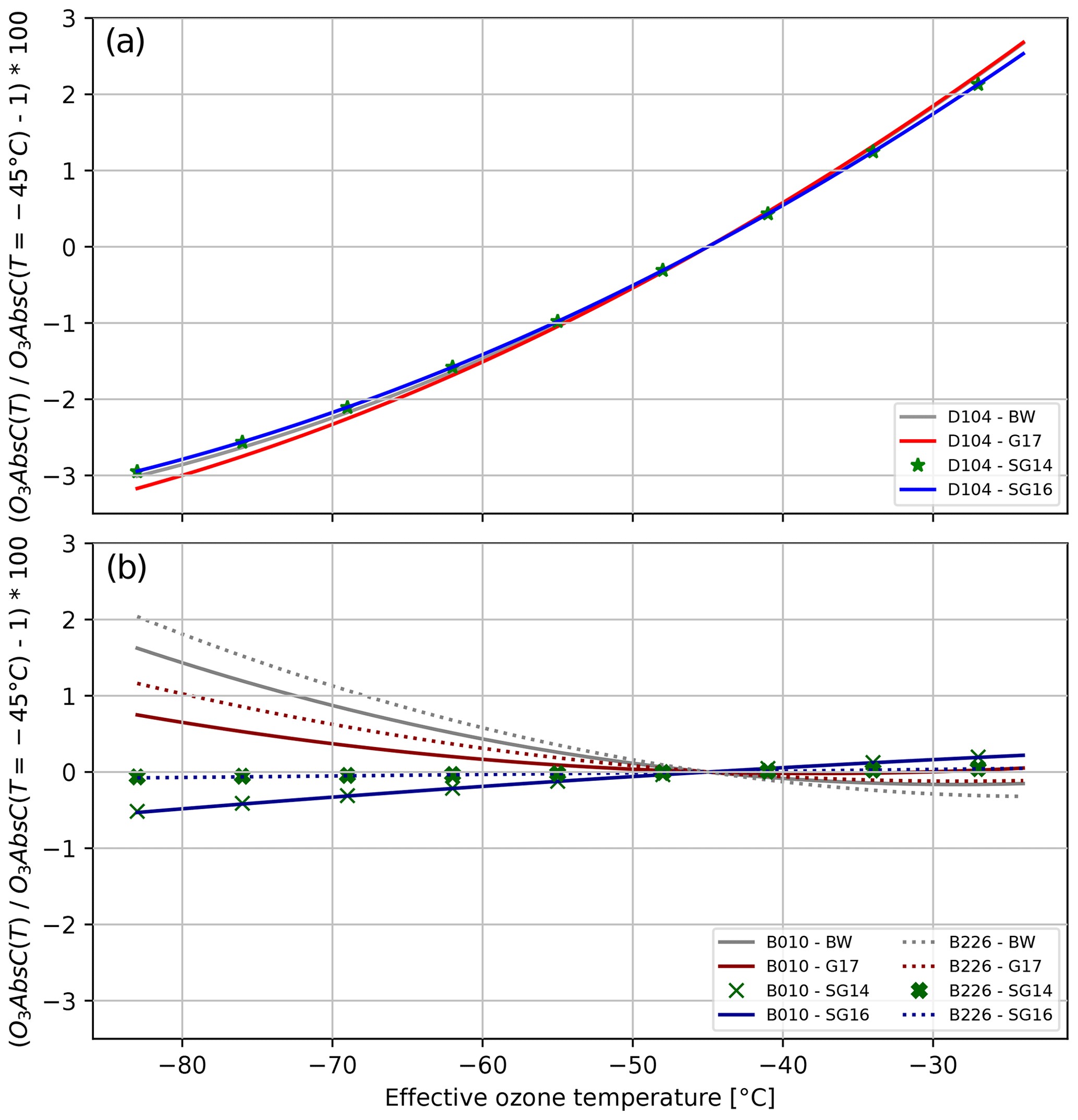
Figure 6 Temperature dependence of the ozone absorption coefficients for different ozone cross-section datasets (SG14, SG16, G17, and BW) for Dobson (D104; a) and Brewer (B010: solid lines; B226: dashed lines; b) instruments. The dependence is calculated relative to the respective absorption coefficient for an effective temperature of −45 °C. For the Dobson instrument, only the results of the AD wavelength pair are shown.

Looking at the temperature dependence of the absorption coefficient Δα in Fig. 6 and at the variations in T_eff in Fig. 5, it becomes quite obvious that the implementation of temperature-dependent ozone cross sections in the operational retrieval algorithm is important, especially for the Dobson instrument. It should reduce the uncertainty in Dobson TOC values by several percent, while improvements for Brewers will generally be smaller (and limited, e.g., by the knowledge of the slit functions of the individual instruments).

3.2 Updated Brewer and Dobson TOC values

The relative difference in TOC when using either the B&P operational ozone absorption coefficients or the new T_eff-dependent absorption coefficients can be calculated using Eq. (14). Table 6 shows the resulting average TOC changes. Generally, the use of the new ozone cross sections leads to increased Dobson TOC values (by 0.8 % to 3.8 %) and to decreased Brewer TOC values (−0.3 % to −1.2 %). The BW dataset provides by far the largest changes for the Dobson instrument. It would increase the differences between the Dobson and Brewer instruments and appears not to be suitable. The three remaining datasets provide mean TOC changes in the range of 0.8 %–1.6 % for the Dobson instrument and −1.2 %– −0.9 % for the Brewer instrument. Among the three datasets, the SG14 and SG16 datasets, along with the Bernhard slit approximation or the TuPS measurement for the Dobson instrument, exhibit the smallest differences compared to the B&P operational dataset.

Table 6 Mean [%] and standard deviation [1σ; %] of the relative difference in TOC between four T_eff-dependent ozone absorption cross sections and the operational B&P dataset with a fixed T_eff for both Brewer and Dobson instruments at Hohenpeissenberg. The differences were calculated using climatological TEMIS T_eff data (1990–2020), and the values show the averaged results for a period of 1 year. The results also correspond to the dashed grey lines in Fig. 7 for the location of Hohenpeissenberg.

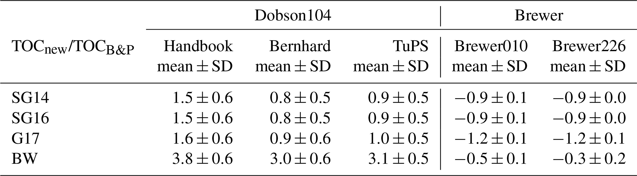
Figure 7 displays corresponding time series for the differences in TOC between the operational B&P-derived values and the SG16 dataset over a period of 2 years and for five different stations from −89.98° to 82.45°. Generally, the new temperature-dependent ozone absorption coefficients lead to larger changes in TOC values at higher latitudes (due to the higher variability in T_eff). In contrast, TOC values close to the tropics vary by less than 1 % when the new ozone cross sections are applied.

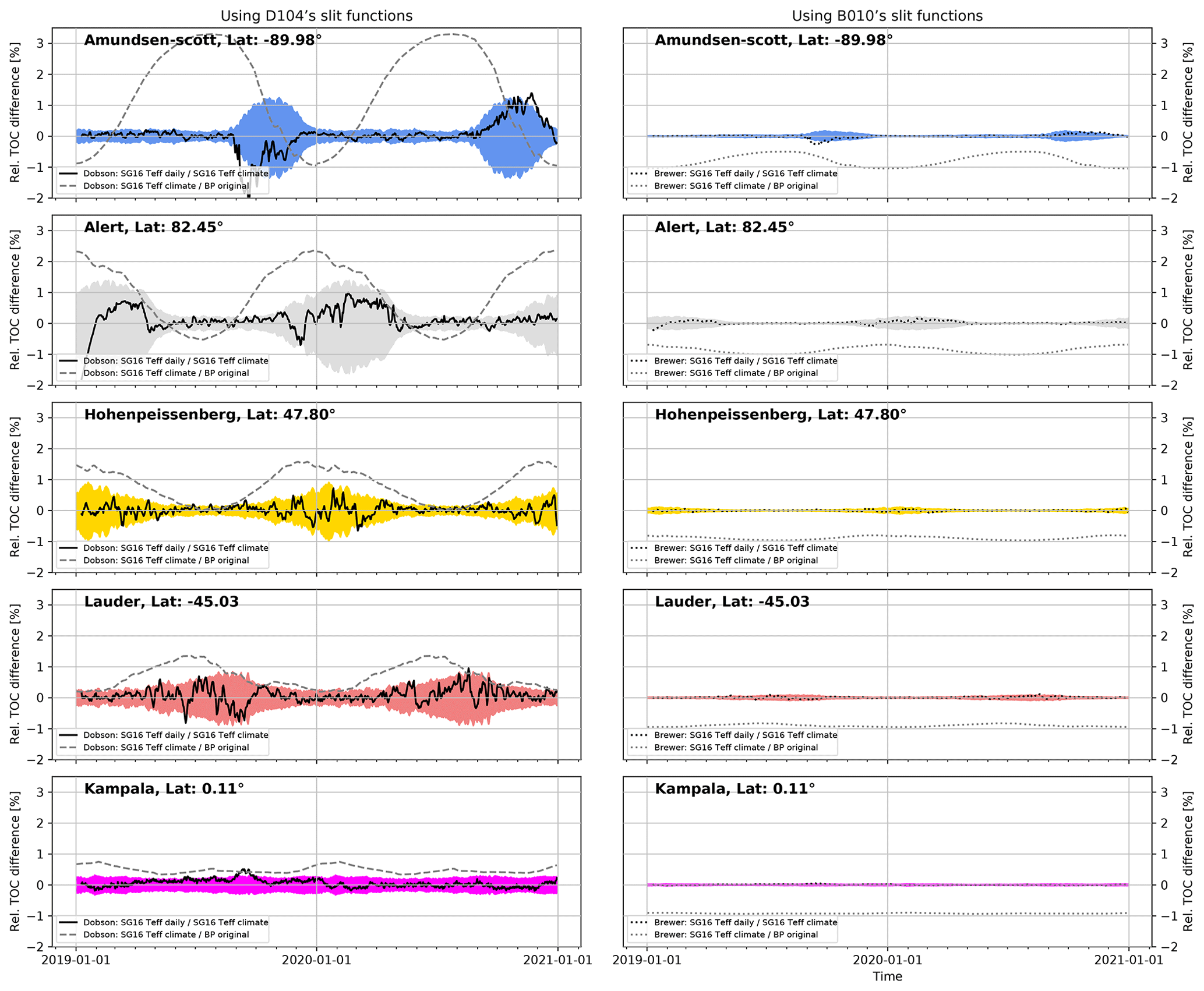
Figure 7 Relative difference in TOC between new T_eff-dependent ozone cross sections (SG16; TEMIS climate) and fixed-temperature B&P cross sections (dashed grey lines) and between daily and climatological values for T_eff (colored shaded regions; SG16 cross section; T_eff daily and climatology from TEMIS). Results are given for five locations and Dobson (left panels) and Brewer (right panels). The shaded areas show the potential difference in TOC (2σ) when using climatological T_eff (1990–2020) instead of daily TEMIS values. Bernhard slit approximation was used for the Dobson instrument. For the Brewer instrument, the slit functions from Brewer010 as described in Table 2 were applied.

Similarly, the impact of using either climatological T_eff values or daily values is much more pronounced for the Dobsons, especially at higher latitudes. Nevertheless, as shown in Fig. 7, for the majority of TOC measurements worldwide, the difference between Dobson TOC values obtained from climatological instead of daily T_eff values is lower than 1 % (2σ). For the Brewers, temperature dependence is much smaller, and there is virtually no difference between using climatological or daily T_eff values.

3.3 Comparison of Brewer and Dobson TOC retrievals

Consistency between TOC measurements from the Dobson and Brewer instruments is crucial for evaluating whether a new ozone cross-section dataset is recommended in this study. Figure 8 shows TOC measurements from Dobson104 compared to those from two Brewer instruments for the different ozone cross-section datasets.

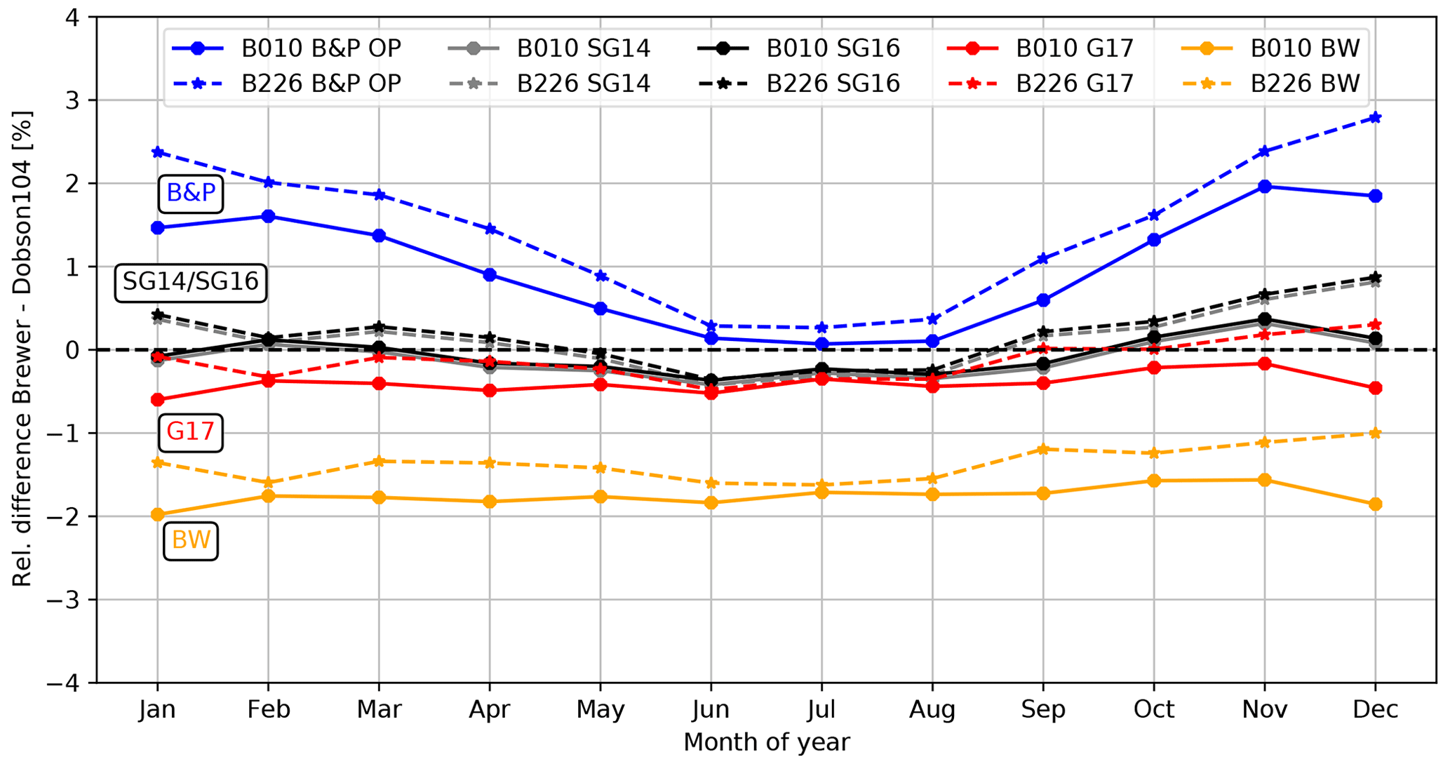
Figure 8 Monthly-mean difference between Dobson104 and Brewer010 and 226 (solid and dashed lines) at Hohenpeissenberg and using the Bernhard slit approximation. The different colors represent the results for the different ozone absorption cross-section datasets.

As already shown in Fig. 1, a seasonal variation is quite prominent for the B&P dataset without T_eff-correction (blue lines). In contrast, the SG14/SG16 cross sections produce almost identical results (black lines) and reduce the seasonal variation to less than ±0.5 %. There is also little difference between the results for Brewer010 and Brewer226 (solid and dashed lines, respectively). The overall difference between Dobson and Brewer is close to zero. The G17 dataset results in a slightly negative Brewer–Dobson average difference and also a very small annual variation (red lines). Much larger mean differences are seen for the B&P OP and BW datasets (blue and orange lines, respectively), albeit with a small annual variation for the BW dataset. On the basis of Fig. 8, it is quite clear that the SG14 and SG16 datasets provide the best overall agreement between Dobson and Brewer measurements.

Gröbner et al. (2021) also identified a large offset for the BW dataset of up to 2.1 % using measured slit functions for their Dobson instrument. Generally, our findings are very similar to those of the previous studies by Gröbner et al. (2021) and Redondas et al. (2014), who, for their stations and instruments, found mean differences for the SG14 dataset in the ranges of 0 % to 1 % and −0.4 % to 0.2 %, respectively. Note that Gröbner et al. (2021) found a larger difference, −1.0 % to −1.5 %, when using their version of the G17 cross sections, whereas in our study the G17 dataset generally performed very well. In part, this difference can be attributed to different Rayleigh coefficients applied (see Eq. 5). Gröbner et al. (2021) used Bodhaine's Rayleigh cross section (Bodhaine et al., 1999), whereas we applied the Rayleigh cross sections from the standard Brewer and Dobson algorithm (Bates, 1984; Komhyr and Evans, 2008). Gröbner et al. (2021) state that applying Bodhaine's values in Davos decreases TOC from Dobson by about −0.5 DU and TOC from Brewer by about −2.4 DU. This may contribute approximately −0.6 % to −0.7 % to the −1.0 % to −1.5 % difference found in Gröbner et al. (2021). The rest seems to be due to an older version of the G17 dataset used by Gröbner et al. (2021). This ambiguity in the G17 dataset and the lack of an official publication lead to the overall recommendation to use the SG16 dataset and not G17.

The choice of slit approximation for the Dobson instrument also influences the comparison. Generally, the best comparison is achieved with the Bernhard approximation or TuPS measurements (see also Fig. S5 in the Supplement). In our case, both outperform the Dobson operations handbook's slit approximation. This is generally consistent with the findings of Gröbner et al. (2021), who, however, obtained slightly better results when using TuPS measurements. Based on our experience and many previous measurements, including a number of Dobson slit measurements worldwide (Gröbner et al., 2021; Köhler et al., 2018), it seems that for a majority of Dobson instruments, the Bernhard et al. (2005) slit approximation is indeed very good, simple, and suitable for the entire network. Due to its ease of implementation and the good results in our study, we recommend the Bernhard slit approximation for Dobson instruments in the operational network.

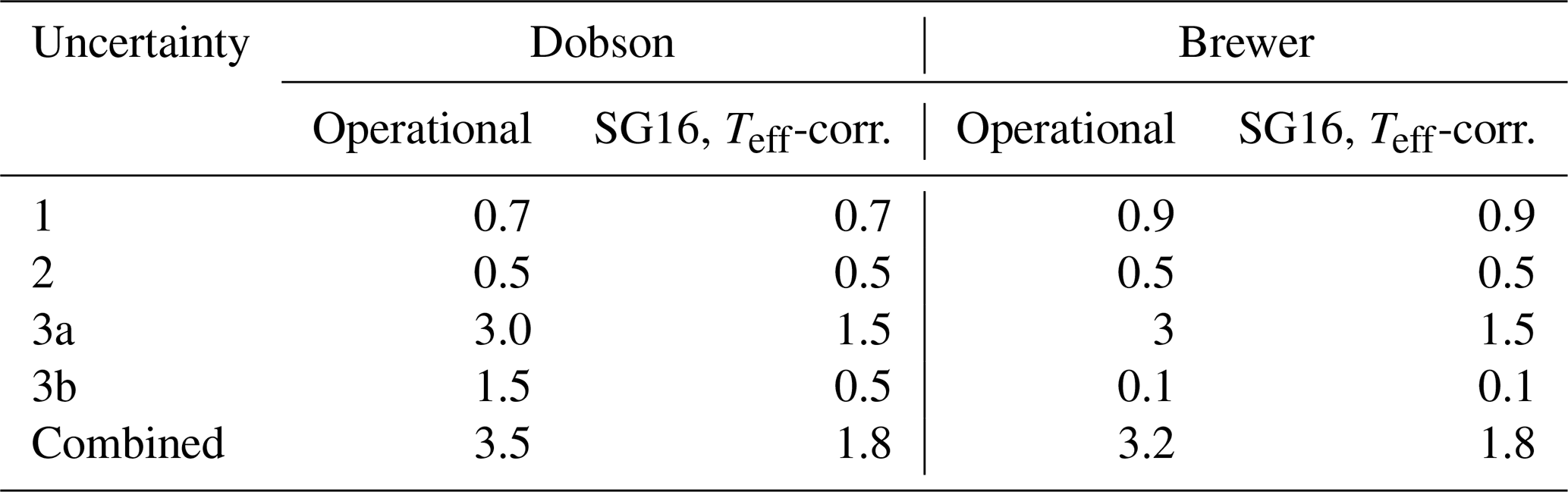
Table 7 Relative standard uncertainty estimation based on the literature (Basher, 1982; Koukouli et al., 2016; Scarnato et al., 2009, 2010; Zhao et al., 2021) and our own study. Uncertainty sources 1, 2, 3a, and 3b correspond to the uncertainties associated with instrumental sources (1), simplified radiative transport assumptions (2), applied cross sections (3a), and T_eff (3b).

Where available, TuPS measurements of Dobson slit functions can result in small improvements (typically on the order of 0.5 % or less), albeit at the cost of additional measurements, additional calculations and much more extensive housekeeping. This may make sense for some specialized research groups, but for the wide network, we feel that the Bernhard slit approximation is adequate and simple to keep track of.

3.4 Uncertainties

A comprehensive analysis of uncertainties for Dobson total ozone measurements is given by Basher (1982); for Brewers, information on uncertainty can be found in different publications (Fioletov et al., 2005; Kerr and McElroy, 1995; Redondas et al., 2018; Zhao et al., 2021). A new assessment of these uncertainties is beyond the scope of this paper. It is the topic of two separate papers in preparation by some of the co-authors. Nevertheless, it is important to consider the various sources of uncertainty here and to determine when further reductions in uncertainty from a single source will not improve the overall uncertainty.

Basher (1982) distinguishes in his analysis between typical “good” instruments or situations (with smaller uncertainties) and “bad” instruments or situations (with large uncertainties). Here, we consider only the good case. In a similar way to Basher, we distinguish between (1) instrumental sources of uncertainty (alignment, calibration, slit functions, instrumental noise, etc.), (2) uncertainty due to simplified radiative transfer assumptions (aerosol and SO₂ interference, ozone layer height, air mass calculation, etc.), and (3) uncertainty due to the used ozone absorption cross sections (3a) and their temperature dependence (3b). All of these uncertainties contain random and systematic parts.

For a typical good Dobson, the instrumental relative standard uncertainties (1) are estimated to be lower than 0.5 % to 1.5 % by Basher (1982). This is consistent with the standard deviation of individual Dobson TOC values observed at Hohenpeissenberg, which is about 0.7 %, and the typical agreement reached in Dobson calibrations, which is also about 0.7 %. It is also consistent with the magnitude of changes due to different wavelengths or slit functions found in this study, which are about 0.5 %, as can be seen in Fig. S5 and Table 7. Similar uncertainties of this type also apply for Brewers. The standard deviation of individual Brewer TOC values observed at Hohenpeissenberg, for example, is about 0.9 %.

Relative standard uncertainties (2), due to the simplified radiative transfer assumptions, are also on the order of 0.2 % to 0.5 % for a good-situation Dobson or Brewer. This study does not address any of these sources of uncertainty, so their values remain unchanged.

The largest improvement coming from this study is in the application of new ozone absorption cross sections with reduced uncertainty (3a) and particularly in addressing the temperature dependence (T_eff) of the ozone cross sections now (3b). Basher quotes an absolute relative standard uncertainty due to the used ozone cross sections of about 3 % and a relative standard uncertainty of about 1.5 % due to neglecting the temperature dependence. The SG16 cross sections recommended here claim a smaller absolute uncertainty (3a) of about 1.5 %, which would apply to both Dobson and Brewer TOC values. The major improvement comes from addressing the temperature dependence (3b, T_eff), which reduces the associated uncertainty for Dobson TOCs from about 1.5 % (compare also the dashed lines in Fig. 7) to less than 0.5 % (compare also the shaded regions in Fig. 7). For the Brewers, the uncertainties associated with T_eff are much smaller and are assumed to be about 0.1 % (see also the right panels in Fig. 7 and Koukouli et al., 2016).

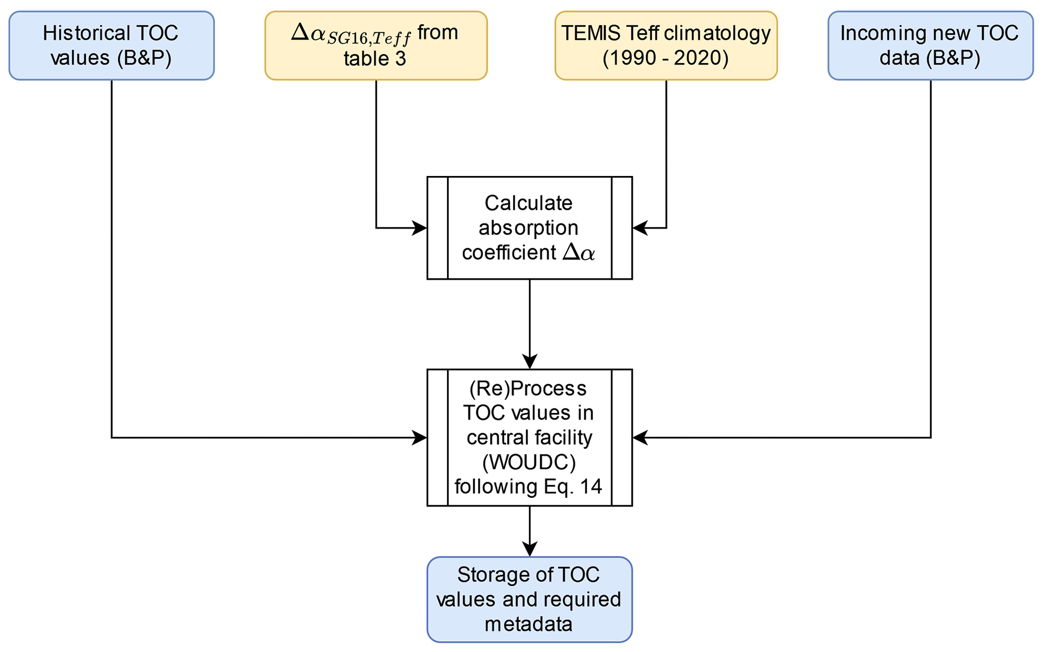
Figure 9 Flowchart illustrating the suggested centralized transition to revised Dobson total ozone column (TOC) time series in the operational network using the new T_eff-dependent SG16 ozone absorption cross sections.

Trends of T_eff are caused by trends in the temperature and ozone profiles. For the period from 1980 to 2000, T_eff trends are on the order of −0.5 to −1 K per decade. For the period from 2000 to 2020, temperature and ozone trends are generally smaller. Assuming a fixed temperature (standard processing) or a climatological temperature (our suggested improved processing) does result in spurious trends of total column ozone. For a Dobson instrument, these spurious total ozone trends are smaller than 0.1 % per decade. Compared to the overall uncertainty for Dobson instruments (about 2 %–3 %), this is small to negligible. For a Brewer instrument, the spurious total ozone trends are almost 1 order of magnitude smaller and are completely negligible. In this context, it is important to also note that the existing standard processing (using one single value for T_eff) and the suggested improved processing (using the climatological annual cycle for T_eff) will provide the same relative TOC trends (% per decade) and almost the same absolute TOC trends (DU per decade). This means that there is no need to revise published total ozone column trends (e.g., those in the WMO/UNEP ozone assessments).

In summary, the improved processing suggested in this paper should reduce the combined relative standard uncertainty in Dobson TOC values from 3.5 % to 1.8 %. For Brewer TOC values, the improvement is smaller, from 3.2 % to 1.8 % (Table 7).

3.5 Recommendations for operational networks

Based on our results and taking into account previous studies (Gröbner et al., 2021; Köhler et al., 2018; Orphal et al., 2016; Redondas et al., 2014, 2018), we recommend the SG16 ozone absorption cross sections for the Dobson and Brewer observing networks. For the Dobson instruments, the slit approximation from Bernhard et al. (2005) should be applied. The correction for the effective ozone temperature should be based on the TEMIS/ECMWF dataset.

• The SG16 (Weber et al., 2016) dataset performs very similarly to the SG14 (Serdyuchenko et al., 2014) dataset which was recommended in the previous studies. However, the SG16 dataset also provides uncertainty budgets, which is useful for further studies.

• The G17 dataset (Gorshelev et al., 2017) provides similar results but introduces a slightly larger mean difference between Dobson and Brewer, compared to SG16. Moreover, no peer-reviewed publication of the dataset exists at the time of this publication.

• The Bernhard slit approximation (Bernhard et al., 2005) outperforms the slit approximation of the Dobson operations handbook (Komhyr and Evans, 2008), which introduces a small bias between Dobson and Brewer measurements. While some studies (Gröbner et al., 2021; Köhler et al., 2018) recommend instrument-specific slit functions (e.g., from TuPS measurements), the application of TuPS measurements did not result in improved consistency between Dobson and Brewer TOC measurements in this study. Moreover, only a very limited number of reliable measured slit functions from Dobson instruments exists to this day. This would delay and complicate the implementation of new ozone cross sections in the operational networks significantly, without a large gain in the accuracy of the resulting TOC values.

• Slightly better results may be achieved, at considerable housekeeping cost, by utilizing measured slit functions (e.g., by the TuPS) for the effective ozone absorption coefficients for Dobson instruments. Here, it is crucial to ensure that the wings of the slit functions are included, particularly at the shorter wavelengths, where the ozone cross sections are large. While this may be the best approach for a few specialized research groups, for much of the operational network, the simple and easily applied Bernhard slit approximation seems good enough and is therefore recommended.

• The TEMIS/ECMWF ozone effective temperature dataset (https://www.temis.nl/climate/efftemp/overpass.php, last access: 11 April 2024) is very well suited for application in the global Brewer and Dobson networks. Differences from measured values from a combination of lidar and ozonesondes are small at the Hohenpeissenberg site, with a standard deviation of only about 1.2 °C for daily values over a time period of 30 years. Climatological values derived from the dataset are sufficient for use in the operational networks. Daily data would not improve the quality of the TOC measurement significantly, with negligible differences in the yearly mean for the majority of observing stations, differences smaller than 1 % for daily TOC data, and larger differences only at high latitudes in winter, where measurements are problematic anyway due to low solar elevation.

The transition to new Dobson TOC values based on SG16 and the TEMIS T_eff climatology should be carried out in a centralized facility, such as the WOUDC. Figure 9 outlines our suggested approach, which would make sure that all critical computations are applied uniformly to both existing historical and incoming new Dobson data. The central processing would use the TEMIS T_eff climatology to calculate new effective absorption coefficients for each reporting measurement location. In addition, the central processing would ensure proper metadata handling (e.g., versioning, applied T_eff, and polynomial function coefficients used for conversion from B&P to SG16).

4 Conclusions

Focusing on Dobson and Brewer total ozone measurements, this study reinvestigated the use of different ozone absorption cross-section datasets, and different ways to account for ozone effective temperatures (T_eff).

Overall, the SG16 ozone cross sections give the most consistent results. At Hohenpeissenberg, the seasonally varying difference between Brewer and Dobson measurements is reduced from close to 0 % in summer and up to 2.5 % in winter to less than ±0.5 % year-round. Therefore, it is recommended to implement the SG16 cross section in both Brewer and Dobson networks. This will provide more consistent and accurate total ozone data.

For the effective ozone temperature (T_eff), satisfactory results are obtained for nearly all reporting stations by simply using TEMIS climatological values. At most stations, very little can be gained using daily T_eff values. For Dobson instruments, improvements typically remain below 1 % (2σ) compared to employing climatological values. In the case of the Brewers, the use of daily T_eff values is entirely unnecessary given the measurements' low sensitivity to temperature variations.

Overall, the uncertainty in total ozone data from the Dobson instrument should improve from currently 3 % to 4 % (due to 1 % to 3 % annual variation in bias) to better than 2 % in the future. Much less can be gained from Brewer total ozone data, where the new cross sections and T_eff data only result in changes on the order of ±0.5 %.